---
category: literaturenote
citekey: ginedevelopmentsustainablemanagementsystem2012
title: Development of a Sustainable Management System for Rural Road Networks in Developing Countries
authors: "Gine, Chamorro; Alondra, Marcela"
year: 2012
date: "2012-02-14 2012-02-14T21:36:39Z"
url: "http://hdl.handle.net/10012/6551"
zotero_key: IJ9EURY4
zotero_storage: L2S97UFW
collections: imporditud
folder: 001_artiklid
firstAuthor: "Gine, Chamorro"
status: converted
---
# Development of a Sustainable Management System for Rural Road Networks in Developing Countries
by
Marcela Alondra Chamorro Giné
A thesis presented to the University of Waterloo in fulfillment of the thesis requirement for the degree of Doctor of Philosophy in Civil Engineering
Waterloo, Ontario, Canada, 2012
©Marcela Alondra Chamorro Giné 2012
# **AUTHOR'S DECLARATION**
| I hereby declare that I am the sole author of this thesis. This is a true copy of the thesis, including any | | |
|-------------------------------------------------------------------------------------------------------------|--|--|
| required final revisions, as accepted by my examiners. | | |
I understand that my thesis may be made electronically available to the public.
\_\_\_\_\_\_\_\_\_\_\_\_\_\_\_\_\_\_\_\_\_\_\_\_\_\_\_\_\_ Marcela Alondra Chamorro G.
# **Abstract**
Rural roads play a crucial role in the economic and social development of societies, linking rural communities to education, health services and markets. During the last decade, considerable efforts have been made to evaluate the benefits of rural road investment in developing countries. Although outputs of these studies have led to a global rethinking of traditional road appraisal methods, limited attempts have been made to integrate these findings to the rural road management process.
For the sustainable management of rural roads, social, institutional, technical, economic and environmental aspects should be considered under a long term perspective. The current practice in developing countries is that only some of these key sustainable aspects are being considered in the management process. In addition, rural roads maintenance management is commonly performed under a short term basis, not considering the life cycle costs and benefits in the economic analysis and project prioritization. Available management tools and studies have essentially focused their efforts on improving technical and economic aspects of low-volume roads. Whereas, the common practice observed in face of limited resources and lack of technical skills is that decisions are made under a political short term perspective.
This research is directed at the development of an applied and practical system for the sustainable management of rural road networks in developing countries. The approach considers the development of all components required by the proposed management system and their integration into a practical and easy-to-use computer tool.
To achieve this goal a sustainable framework for rural roads management was first developed, where system components and modules were defined. A network level condition evaluation methodology was selected and validated. Long term condition performance models were calibrated from the probabilistic analysis of field data. Optimal maintenance standards were developed under a cost-effectiveness approach. A long term prioritization procedure was developed to account for sustainable aspects of rural roads in the management process. A computer tool was finally developed to integrate the system components and display them in a friendly interface for potential users. The tool was programed in Visual Basic, considering Microsoft Excel interface. The computer tool considers the four system components: Input Data, System Modules, Network Analysis Interface and Output Data. System Modules include Condition Performance Module, Network Maintenance Module and Long Term Prioritization Module. For each of the system components and modules a separate worksheet has been included in the computer tool. The tool is centered on the Network Analysis Interface, which interacts with the other three system components. The user enters network data in the Input Data interface and may adjust information in System Modules considered if the network under study has differences to predefined conditions of. Adjustments to System Modules can be performed by the user, however it is advised that prior calibration is required for the successful analysis of the network.
The management system was applied and validated in two rural road networks in developing countries located in Chile and Paraguay. Sensitivity analysis was carried out to assess the impacts of input parameters in the performance of developed system. As a result of the research an adaptable and adoptable sustainable management system for rural networks was developed to assist local road agencies in developing countries.
# **Acknowledgements**
I would like to begin by expressing my gratefulness to my supervisor, Professor Susan Tighe, for her continuous support and precious guidance during the last four years. It has been a gift to know you and a pleasure to work and learn from you.
I would also like to thank my examination committee members, Professor Ralph Haas, Professor Carl Haas, Professor Alexander Penlidis and Dr. Cesar Queiroz for taking their time to review my thesis.
I would like to acknowledge the help of the Municipality of Portezuelo in Chile, providing data and resources for the field evaluations. I would specially like to acknowledge the support from my friends Tomás Plaza, Raquel Bustamante and their families, for sharing precious information and moments during field visits. I would also like to thank the support provided by the Major of the Municipality, Modesto Sepúlveda, and the keen collaboration of Bernardo Molina, Pedro Toro, Ricardo Ortega, Mabel Cartes and Juana Hermosilla.
The support of the Ministry of Public Works and Communications of Paraguay (MOPC), who provided data and resources for the development of the case study held in Paraguay, is gratefully acknowledged. In particular, I would like to acknowledge Alelí Osorio and her family, for their kindness during my stay in Paraguay, and to the dedicated contributions of Ing. Luis Ugarte, Ing. Roberto Bogado and Mariela Gauto.
I would like to make a special recognition to my friend Nestor Rojas who altruistically provided his knowledge, guidance and precious time for the development of the computer tool.
I would like to thank the CPATT team and all who have made my stay at the University of Waterloo a great memory. Especially, to the support and friendship of Vimy Henderson, Jodi Norris, Rabiah Rizvi and Laura Bland.
To my friends, where destiny crossed our ways in Waterloo to share beautiful moments during these years of study. To Amparo Edwards, Néstor Rojas, Rita López, Leandro Becker, Sandra Céspedes, Valentina Rodriguez, Maria Cristina Maal and Orietta Beltrami.
I would like to express my gratefulness to the Government of Chile, which through the Scholarship "Presidente de la República" funded my PhD studies. Also to the financial support of the Natural Sciences and Engineering Research Council of Canada (NSERC).
Finally I would like to thank my family for all their love, patience and support.
# **Dedication**
I would like to dedicate this work to my husband Alvaro and my daughter Marina, and to my parents Loly and Hernán. None of this would have been possible without your support.
| Abstract iii | |
|---------------------------------------------------------------------------------------------|--|
| Acknowledgements v | |
| Dedication vi | |
| Table of Contents vii | |
| List of Figures x | |
| List of Tables xi | |
| List of Abbreviations xiii | |
| Chapter 1 Introduction 1 | |
| 1.1 Background 1 | |
| 1.2 Problem Statement and Research Approach 7 | |
| 1.3 Research Hypotheses 8 | |
| 1.4 Objectives and Scope 8 | |
| 1.5 Research Methodology 8 | |
| 1.6 Thesis Organization 11 | |
| Chapter 2 Literature Review 13 | |
| 2.1 Purpose of the Chapter 13 | |
| 2.2 Rural Roads Characteristics 13 | |
| 2.3 Unpaved Roads Performance and Maintenance 14 | |
| 2.4 Economic Evaluation and Road Maintenance Prioritization 23 | |
| 2.5 Management Systems and Tools Applied to Rural Roads 30 | |
| 2.6 Limitations of Current State-of-the-Practice and Opportunities for Improvement 33 | |
| Chapter 3 Proposal of a Sustainable Management System for Rural Road Networks in Developing | |
| Countries 36 | |
| 3.1 Introduction 36 | |
| 3.2 Sustainable Approach 36 | |
| 3.3 Integrated Framework for the Sustainable Management of Rural Roads 38 | |
| 3.4 Proposal of a Sustainable Management System for Network Level Management 41 | |
| 3.5 Summary of the Chapter Findings 46 | |
| Chapter 4 Experimental Design and Data Collection 48 | |
| | |
| 4.2 Experimental Design 48 | |
|---------------------------------------------------------------------------------------------|--|
| 4.3 Selection of Rural Road Networks 55 | |
| 4.4 Data Collection 58 | |
| 4.5 Data Summary 62 | |
| Chapter 5 Development of the Condition Performance Module 66 | |
| 5.1 Introduction 66 | |
| 5.2 Validation of UPCI Methodology 66 | |
| 5.3 Development of Condition Performance Models 68 | |
| 5.4 Maintenance Effects on Roads Condition 73 | |
| 5.5 Validation of Unpaved Roads Condition Performance Models and Maintenance | |
| Recommendations 76 | |
| 5.6 Summary of the Chapter 77 | |
| Chapter 6 Development of the Network Maintenance Module 78 | |
| 6.1 Introduction 78 | |
| 6.2 Development of Maintenance Strategies 78 | |
| 6.3 Development of Optimal Maintenance Standards 82 | |
| 6.4 Summary of the Chapter 89 | |
| Chapter 7 Development of the Long Term Prioritization Module 91 | |
| 7.1 Introduction 91 | |
| 7.2 Development of a Sustainable Priority Indicator 91 | |
| 7.3 Prioritization Procedure 93 | |
| 7.4 Summary of the Chapter 96 | |
| Chapter 8 Application and Validation of the Sustainable Management System for Rural Road | |
| Networks 97 | |
| 8.1 Introduction 97 | |
| 8.2 Development of a Computer Tool 97 | |
| 8.3 Application and Validation of the Management System and Computer Tool 101 | |
| 8.4 Sensitivity Analysis of the Management System 116 | |
| 8.5 Findings from the Application and Validation of the Management System and Computer Tool | |
| 121 | |
| Chapter 9 Conclusions and Recommendations 123 | |
| | |
| 9.2 Recommendations 127 | |
|---------------------------------------------------------------------------|--|
| 9.3 Future Research and Developments 128 | |
| References 129 | |
| Appendix A Recommendations for Project Level Analysis 139 | |
| Appendix B Example of Roads Structural Capacity Evaluations 141 | |
| Appendix C Maintenance Treatment Costs and Costs per Budget Scenario 151 | |
| Appendix D Sample of Condition Survey Sheet 153 | |
| Appendix E Case Studies Inventory and Field Data 154 | |
| Appendix F Data Analysis: Development of Condition Performance Module 164 | |
| Appendix G Data Analysis: Development of Network Maintenance Module 174 | |
| Appendix H Computer Tool Overview 190 | |
| Appendix I Application and Validation of the Management System 192 | |
| Appendix J Sensitivity Analysis of the Management System 200 | |
# List of Figures
| Figure 1.1 Road Hierarchy and Function (SADC, 2003) 2 | |
|----------------------------------------------------------------------------------------------|--|
| Figure 1.2 Multifunctional Nature of Roads (SADC, 2003) 2 | |
| Figure 1.3 The Elements of Rural Development (Lebo, 2000) 3 | |
| Figure 1.4 Features of Rural and National Roads (Lebo, 2000) 5 | |
| Figure 1.5 SADC Framework for Sustainable Provision of Low Volume Roads (SADC, 2003) 6 | |
| Figure 1.6 Research Methodology 9 | |
| Figure 2.1 Percentage of Rural Population with All-Season Access (Plessis-Fressard, 2007) 28 | |
| Figure 3.1 Integrated Management Framework 38 | |
| Figure 3.2 Proposed Network Management System 42 | |
| Figure 4.1 Location of the Selected Road Network in Chile 55 | |
| Figure 4.2 Selected Road Network in Paraguay 57 | |
| Figure 5.1 Validation of UPCI Methodology 67 | |
| Figure 5.2 Condition Performance Curves for Strong Structure Roads or Gravel Roads 72 | |
| Figure 5.3 Condition Performance Curves for Weak Structure Roads or Earth Roads 72 | |
| Figure 5.4 Validation of Gravel Curves: UPCI observed vs. calculated 76 | |
| Figure 5.5 Validation of Earth Curves: UPCI observed vs. calculated 77 | |
| Figure 7.1 Short and Long Term Prioritization Procedure 94 | |
| Figure 8.1 Network Analysis Process 99 | |
| Figure 8.2 Gravel vs. Earth Roads Performance: Chile Case Study 104 | |
| Figure 8.3 Gravel Roads Performance: Chile Case Study 105 | |
| Figure 8.4 Earth Roads Performance: Chile Case Study 105 | |
| Figure 8.5 Maintenance Costs: Chile Case Study 107 | |
| Figure 8.6 Gravel vs. Earth Roads Performance: Paraguay Case Study 111 | |
| Figure 8.7 Gravel Roads Performance: Paraguay Case Study 112 | |
| Figure 8.8 Earth Roads Performance: Paraguay Case Study 112 | |
| Figure 8.9 Maintenance Costs: Paraguay Case Study 114 | |
| Figure 8.10 Network Performance: Chile vs. Paraguay Case Studies 116 | |
| Figure 8.11 Effects of Climate on Network Performance 118 | |
| Figure 8.12 Effects of Budget Levels on Network Performance 119 | |
# **List of Tables**
| Table 2.1 Maintenance Categories and Activities 18 | |
|---------------------------------------------------------------------------------------|--|
| Table 2.2 Guidelines for Levels of Serviceability (NITRR, 2009) 19 | |
| Table 2.3 Estimation of IRI on the basis of comfortable travel speed (NITRR, 2009) 20 | |
| Table 2.4 Economic Evaluation Methods 24 | |
| Table 2.5 Priority Programming Methods 25 | |
| Table 4.1 Traffic Levels 53 | |
| Table 4.2 Factorial for the development of the Condition Performance Module 54 | |
| Table 4.3 Factorial for the development the Network Maintenance Module 54 | |
| Table 4.4 Condition Limits for Unbound Gravel Roads 60 | |
| Table 4.5 Condition Limits for Stabilized Gravel Roads 60 | |
| Table 4.6 Condition Limits for Earth Roads 60 | |
| Table 4.7 Conditions Assigned to Extreme Defect Values 60 | |
| Table 4.8 Summary of Gravel Road Condition: Chile Case Study 63 | |
| Table 4.9 Summary of Earth Road Condition: Chile Case Study 64 | |
| Table 4.10 Summary of Paraguay Network Condition 65 | |
| Table 5.1 Corrected Conditions for Extreme Defect Values 67 | |
| Table 5.2 Gravel Condition Summary Table 69 | |
| Table 5.3 Earth Condition Summary Table 69 | |
| Table 5.4 Gravel Cumulative Probability Transition Matrix 70 | |
| Table 5.5 Earth Cumulative Probability Transition Matrix 70 | |
| Table 5.6 Calculation of Maintenance Effects 74 | |
| Table 5.7 Maintenance Strategies and UPCI effects Recommended for Gravel Roads 74 | |
| Table 5.8 Maintenance Strategies and UPCI effects Recommended for Earth Roads 75 | |
| Table 6.1 Maintenance Treatments per Funding Levels 80 | |
| Table 6.2 Maintenance Strategies for Gravel Roads 81 | |
| Table 6.3 Maintenance Strategies for Earth Roads 81 | |
| Table 6.4 Maintenance Treatment Costs 82 | |
| Table 6.5 Application Ranges and Performance Jump Values for Gravel Roads 83 | |
| Table 6.6 Application Ranges and Performance Jump Values for Earth Roads 83 | |
| Table 6.7 Maximum Condition Levels per Strategy 84 | |
| Table 6.8 MCE Analysis for Gravel Roads 87 | |
| Table 6.9 MCE Analysis for Earth Roads 87 | |
|--------------------------------------------------------------------------------------|--|
| Table 6.10 Optimum Standards for Gravel Roads 88 | |
| Table 6.11 Optimum Standards for Earth Roads 89 | |
| Table 8.1 Computer Tool Input Data: Chile Case Study 102 | |
| Table 8.2 Required Funding per Budget Level: Chile Case Study 103 | |
| Table 8.3 Computer Tool Input Data: Paraguay Case Study 108 | |
| Table 8.4 Adjusted Maintenance Standards: Paraguay Case Study 109 | |
| Table 8.5 Required Funding per Budget Levels: Paraguay Case Study 109 | |
| Table 8.6 Funding per Budget Levels, Second Analysis Period: Paraguay Case Study 110 | |
| Table 8.7 Summary of Sensitivity Analysis: Climate 117 | |
| Table 8.8 Summary of Sensitivity Analysis: Budget 118 | |
| Table 8.9 Summary of Sensitivity Analysis: Discount Rate 120 | |
# **List of Abbreviations**
AADT Average Annual Daily Traffic
BCA Benefit Cost Analysis BAA Basic Access Approach CBR California Bearing Ratio CEA Cost Effectiveness Analysis
DFID Department for International Development
ERR Economic or Internal Rate of Return
FPS Ficha de Protección Social GDP Gross Domestic Product
HDM-III Design and Maintenance Standards Model HDM-4 Highway Development and Management Model
IDA International Development Association
IRI International Roughness Index
ISOHDM International Study of Highway Development and Management Tools
LCCA Life Cycle Cost Analysis
MOP Ministry of Public Works of Chile
MOPC Ministry of Public Works and Communications of Paraguay
RED Roads Economic Decision Model RONET Road Network Evaluation Tools
RAI Rural Access Index
SADC Southern African Development Community
TRL Transportation Research Laboratory UPCI UnPaved Road Condition Index URCI Unsealed Road Condition Index
VOC Vehicle Operating Costs
# **Chapter 1**
# **Introduction**
# **1.1 Background**
#### **1.1.1 Definition of Rural Roads**
Rural roads have been defined under various perspectives, depending on the level of development of a country and the specific technical and socio-economic aspects of the road. The International Labour Organization defines rural roads as all publicly owned roads whose primary purpose is to provide direct access for the rural villages and communities to economic and social services (ILO, 2010). This definition may be insufficient as it may be neglecting the importance of roads, tracks and paths owned by local governments and communities, commonly known as Rural Transport Infrastructure (Lebo, 2000). A broader perspective is considered by the International Development Association (IDA), the World Bank's fund for the world poorest countries, which defines rural roads as all other roads than main roads (IDA, 2007). This comprehensive definition may differ significantly between countries according to their socio-economic condition. In developed countries, rural roads are generally structurally designed low traffic facilities connecting towns with low populations with the primary and secondary network. Meanwhile, in developing countries rural roads are commonly unpaved lowvolume roads designed to meet the social and economic needs of the rural population (Plessis-Fraissard, 2007). The rural network in developing countries commonly represents 80% of the total road network lengths, carries 20% of the total motorized traffic, but provides access to the majority of population to main roads and social networks (Raballand, 2010).
In this thesis, rural roads are considered as unbound gravel and earth roads, paths and tracks serving low volume traffic, less than 300 Average Annual Daily Traffic (AADT) and non-motorized traffic (including haulage carts, bicycles and pedestrians), designed to meet the social and economic needs of the rural population in a developing country. With this, production roads specially designed for exploitation of natural resources, such as forestry and mining roads, are excluded from the analysis.
Considering a three level hierarchy network, rural roads are usually secondary and tertiary/access roads in rural areas as illustrated in Figure 1.1 (SADC, 2003). Tertiary/access roads are tracks or very simple earth roads that begin at the farm/village level and connect the rural population to the secondary network. These are usually seasonal roads with low serviceability levels transited by nonmotorized traffic and motorized traffic at low speeds. Secondary roads are earth or basic gravel roads which serve the needs of low-volume traffic of conventional vehicles and non-motorized vehicles. These roads are connected to the primary network, which are engineered all-season roads that present higher levels of heavy load motorized traffic and connect cities and towns (Tighe, 2007).

**Figure 1.1 Road Hierarchy and Function (SADC, 2003)**
The World Road Association Committee for Appropriate Development - PIARC C20, has defined accessibility as a measure of how easy a place is to get to (Tighe, 2000). A place is accessible when a person can get to it within an acceptable outlay of time, effort and resources, considering affordable means of transport. Mobility is a measure of the ease with which people can move through the road network. Places become more accessible when the population is more mobile. As illustrated in Figure 1.2, the hierarchy or category of a rural road is related to its role in providing access and mobility to the population it serves. Rural roads at the tertiary level serve as an access link in a road transport chain with one end in the agricultural fields or villages and the other in the town market. Primary roads serve as a mobility link in the road transport chain from the main highway network to the local market. At the secondary level, rural roads have a double function, providing access and mobility to population, goods and services (SADC, 2003).

**Figure 1.2 Multifunctional Nature of Roads (SADC, 2003).**
#### **1.1.2 2 Rural Roa ads and Deve elopment**
Rura comm allev infra appr al roads play munities to viation in dev astructure, p ropriate macr y a crucial ro education, h veloping cou roductive se roeconomic f ole in the ec health servic untries depen ectors, socia framework an conomic and es and mark nds on the sy al and econ nd good gove d social deve kets. As pres ynergy and s omic servic ernance polic elopment of sented in Fig simultaneous es. All of cies (Lebo, 2 societies, lin gure 1.3, rur s improveme these provid 2000). nking rural ral poverty ent of rural ded by an
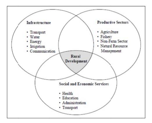
**Figure 1.3 3 The Eleme ents of Rura l Developme ent (Lebo, 20 000)**
Re poor betw study incre deve ecent studies r countries. ween the exte y found that easing incom elopment or h s have evalu In Asian an ent of the ro expenditure me. This impa health (Fan, 1 uated the pos nd African c oad network on rural road act was high 1999) sitive impact countries, st and expendi ds presented her than that of rural roa tudies have iture on road the highest im observed fro ads investme demonstrate ds with incom mpact in redu om crops irri nt and devel ed a close r me growth. ucing rural p gation, educa lopment of relationship In India, a poverty and ation, rural
Re 2004 enro imm girls 27% poor In th long egarding edu 4) reveal that lment rates munization lev living in vil % for those liv r accessibility he presence o ger required ( ucation and t the presenc , improvem vels of the p llages with a ving in villag y conditions, of all-season Plessis-Frais health, studi e of an all-se ment in edu population an all-season roa ges without girls have th roads, butan ssard, 2007). ies held in P eason rural ro ucation qual nd more birth ad access pre all-season ro he daily duty ne gas is affo Pakistan (Es oad in a villa lity, higher hs assisted b esent school e oad access. T y of collecting ordable and, sakali, 2005 age is associa use of he by a skilled a enrolment ra This is expla g firewood fo therefore, fir ) and Moroc ated with hig ealth servic attendant. In ate of 41% co ined by the for cooking an rewood colle cco (Levy, gher school es, higher particular, ompared to fact that in nd heating. ection is no
In road n the case of ds resulted in f economic g an increase growth, it wa of 5.68 Yua as demonstra an of rural no ated in China on-farm gross a that every s domestic p Yuan invest product (GDP ted in rural P) and 1.57 Yuan of agricultural GDP (Fan, 2004a). In Vietnam, a close relationship between the level of economic activity and the extent of the rural road network was observed. It was found that, for every Dong invested in roads, 3.01 Dong of agricultural production value would be produced (Fan, 2004b)
Regarding household consumption, Jalan and Ravallion (2002) found that kilometers of rural road per capita were one of the main explanations of household consumption growth in southern China. Similar conclusions were drawn in a study held in Ethiopia, where higher consumption growth was attributed to road quality improvement, especially concerning accessibility in the wet season (Dercon, 2005).
Negative impacts have also been observed in some cases due to poor design and/or management of rural road projects. These include involuntary resettlement, increased traffic accidents and environmental effects. It is therefore necessary that rural roads should be managed accordingly, supported by consistent public policies and suitable management systems.
#### **1.1.3 Rural Roads Management in Developing Countries**
Rural roads management can be defined as the process that covers all those activities involved in providing and maintaining rural roads at an adequate level of service. This considers the identification of optimum strategies at various management levels and the implementation of these strategies (Haas, 1994).
The management process is performed under three operational levels: project, network and strategic levels. At the project level, technical decisions are made towards the design, construction and maintenance of specific road projects. The main purpose of network management level is the development of a priority program and schedule of work to maintain a road network under available budgets. Finally, at the strategic level pavement performance and maintenance decisions are communicated to senior managers and the public.
As presented in Figure 1.4, rural road networks are commonly managed by communities, municipalities, local governments and, up to some extent, by provincial and central governments (Lebo, 2000). Although rural roads asset value is small compared to national and provincial road networks, the extent of rural networks represent the main proportion of a nation's roads system. In the practice, agencies responsible of rural roads management in developing countries lack of enough budget and resources to manage the network properly. Technical skills of highway engineers are limited and practical decision-making tools for preparing road maintenance programs are not available. In addition, many roads are not classified, especially at the lower level of the networks, where a clear distinction between roads, tracks and paths may not be available (World Bank, 2007). Given this, agencies are unable to evaluate the overall condition of the road network, quantify the socio-economic effects associated to a poor network condition and, therefore, accounting to the government and the public the need for investing in rural roads maintenance (Mushule, 2004).

**Figure 1.4 Features of f Rural and N National Ro oads (Lebo, 2 2000)**
In road majo the H the I deve cons cons syste servi man netw nternational o d managemen or internation Highway Des ISOHDM stu elopment of t siders three siders perform em is centere ice of a ro agement wh works with ve organizations nt systems an nal study wa sign and Mai udy was deve the Highway levels of an mance model ed on the qu ad or netwo here traffic r ery low traffi s and resear nd decisionas carried out intenance Sta eloped to enh y Developme nalysis, nam ls for paved a uantification ork. This ap related econo ic volumes. ch institution -making tool t by The Wo andards Mod hance and up nt and Mana mely project, and unpaved of benefits approach is omic decisio ns have mad ls for low in orld Bank wh del, HDM-III pdate HDM-I agement Mod programme d roads. The e and costs to suitable for ons prevail; de important ncome econo hich resulted I (Watanatad III system. Th del, HDM-4 e and strateg economic ana o road users r primary an however, it t efforts in d omies. During d in the deve da, 1987). In he study resu (Kerali, 2000 gic analysis alysis perform caused by th nd secondar can be insu developing g 1980's a lopment of the 1990's ulted in the 0). HDM-4 . The tool med by the he level of ry network ufficient in
So to lo man Deci (Arc The main ome attempts ow-volume r agers with l ision model chondo-Calla approach o ntenance proj s have been m road network limited resou (RED) (Arc ao, 2007) dev of these met jects under a made to adju ks. These ha urces and tec chondo-Calla veloped by th thodologies, a vehicle oper ust HDM-4 a ave resulted chnical skills ao, 1999) an he Sub-Sahar however, h rative cost pe and other man d in simplifie s. Examples nd Road Ne ran Africa Tr has still cen erspective. nagement too ed tools suit of these are twork Evalu ransport Poli ntered the ec ols for their a table for ag e the Roads uation Tools cy Program ( conomic eva application encies and Economic (RONET) (SSATPP). aluation of
#### **1.1.4 Sustainable Management of Rural Roads**
The Southern African Development Community (SADC), in its Low-Volume Sealed Roads Guidelines, proposed that sustainable systems should include the seven dimensions presented in Figure 1.5. The approach considers political, social, institutional, technical, economic, financial and environmental aspects. The guidelines suggest that long term goals of sustained economic growth and poverty alleviation in the region have failed in the past because one or more of these seven key dimensions were missing or inadequate (SADC, 2003). Moreover, a sustainable management approach has to consider these key aspects throughout the whole life cycle of the rural road network.
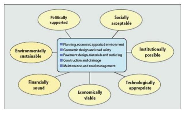
**Figure 1.5 SADC Framework for Sustainable Provision of Low Volume Roads (SADC, 2003)**
The problem that arises from the analysis of the current practice is that only some of these seven key sustainable aspects are being considered in the management process. In addition, rural roads maintenance management is commonly performed under a short term basis, not considering the life cycle costs and benefits in the economic analysis and project prioritization. Available management tools and studies have essentially focused their efforts on improving technical and economic aspects of low-volume roads. Whereas, the common practice observed in phase of limited resources and lack of technical skills is that decisions are made under a political short term perspective.
Regarding social aspects, considerable effort has been made during the last decade to evaluate and quantify the costs and benefits of rural road investments in developing countries. Several studies have applied and developed methods for the socioeconomic impact assessment and the selection of rural road investments (Grootaert, 2002; van de Walle, 2000; Asian Development Bank, 2002). The focus of these studies, however, has been centered on the quantification of socioeconomic direct and indirect effects rather than on the inclusion of social aspects in the management process of rural roads. In addition, the valuation process has primarily been applied on a per case basis. Although outputs of these studies have led to a global reassessment of traditional road appraisal methods, limited efforts have been made to integrate these findings to the rural road management process where they can effectively better quantify the overall impacts of investments at a network and strategic level. Outcomes from these case studies have been treated as local cases and analyzed from a specific sociological and economic point of view. In addition, the level of detail required for these case studies has been extensive and has resulted in huge expense and limited ability to apply them at the network level.
### **1.2 Problem Statement and Research Approach**
The aforementioned discussion cites several limitations of the state-of-the-practice on rural roads management in developing countries. The main problems observed are:
- Available management tools commonly require detailed data of roads condition, structure and materials. Evaluations of road deterioration usually demand trained operators and automated equipment, not commonly available in developing countries. In addition, comprehensive field evaluations are required, which may not be affordable for network level application in developing countries. To overcome these limitations, several agencies have developed subjective rating methods for unpaved roads; however, their reliability is questioned especially when applied by personnel with low technical skills (Sayers, 1986; Archondo-Callao, 1999; Namur, 2009).
- Performance and economic models considered by available management tools need to be calibrated to local conditions. The calibration process in most cases is complex and requires comprehensive data collection. This can be expensive and technically challenging to implement for local agencies. However, if models are not suitably adapted to local conditions, important errors can be induced in the evaluation process.
- Most management tools perform economic analysis and prioritization of maintenance projects considering savings in vehicle operating costs (VOC) and road user travel time costs (TTC). This approach may be insufficient in rural roads having low volume traffic, where, socio-economic costs and opportunities for the rural population may be of more relevance. However, combining VOC and TTC with socio-economic benefits under a traditional costbenefit analysis methodology may be unrealistic given the difficulties of quantifying social values in monetary terms. (Lebo, 2000).
- Limited systems are available that can be easily operated by local agencies in charge of rural roads management in developing countries. With limited resources and lack of technical tools, management decisions are often made from a political short term approach instead of a sustainable mid- to long- term perspective.
Given the state-of-the-art and state-of-the-practice of rural roads management in developing countries, it can be stated that there is no management system currently available that can overcome the four problems described above. Therefore, this research is directed at the development of an applied and practical system for the sustainable management of rural road networks in developing countries. The approach considers the development of all components required by the proposed management system and to integrate them in a practical and easy-to-use computer tool. The main components required to achieve this goal include: network level condition evaluation methodology, long term condition performance models, cost-effective maintenance standards, sustainable prioritization methodology and integrated rural roads management tool.
#### **1.3 Research Hypotheses**
The hypotheses proposed for this research program are as follows:
- Unpaved roads condition performance can be modeled from the probabilistic analysis of field evaluations.
- Maintenance standards for different climates, traffic levels and budgetary scenarios can be optimized for rural roads in developing countries using cost-effectiveness analysis.
- The management of rural road networks in developing countries can be improved by incorporating sustainable aspects in the prioritization process of maintenance projects.
#### **1.4 Objectives and Scope**
The main objective of the research is to develop a sustainable rural roads management system for agencies in developing countries, which considers practical and adaptable components applicable at the network management level.
The research is directed at improving the management process of unpaved road networks that serve rural populations in developing countries. Considering this, the scope is to define a system that can be used by agencies in charge of the network management, considering available resources and their technical skills. The system should be adaptable to different scenarios, in terms of climate, budget, traffic and road types, among other variables.
To accomplish the main objective, the following specific objectives involved include:
- Develop a sustainable framework for rural road networks management.
- Select and validate an unpaved roads condition evaluation methodology and indicator applicable at the network level.
- Calibrate and validate condition performance models for earth and gravel roads representative to different climates.
- Develop and validate optimal maintenance standards considering different climates, traffic and budgetary scenarios.
- Develop a sustainable prioritization methodology for rural road networks maintenance
- Integrate the developed system components in a simplified management tool.
- Validate the management system in two road networks located in Chile and the other in Paraguay.
#### **1.5 Research Methodology**
The research methodology considers twelve activities as presented in Figure 1.6. These activities are described in detail as follows.

**Figure 1 1.6 Research h Methodolo ogy**
- 1. Lite exis Sust iden deve perf mob opti erature Revie sting manag tainable aspe ntified. This eloping coun formance mo bility valua imization tech ew: Available gement prac ects and the included t ntries, unpav odelling tech ation metho hniques and e literature w tices of ru e required sy the assessme ved roads c hniques, soc ods, availab economic an was reviewed ural road ne ystem comp ent of rural condition eva cioeconomic ble mainten nalysis metho d to identify t etworks in onents were l roads man aluation and impact anal nance treatm ods, among o the main defi developing e studied in nagement pr d performanc lysis, access ments and others. iciencies in countries. detail and ractices in ce models, sibility and standards,
- 2. Dev Cou betw then sust how cons man com fram velopment of untries: A sy ween the stra n centered o tainable aspe w system com sider sustain nagement sy mponents dev mework. f a Sustainab ystematic an ategic, networ on the devel ects to be co mponents ha nable aspect stem is a re veloped for n ble Managem nd comprehe rk and projec lopment of nsidered at t ad to be dev ts in the pr esult of the network leve ment Framew ensive frame ct manageme system com the network veloped, how rioritization integration el applicatio work for Rura ework consi ent levels wa mponents and level. This i w they shoul of roads m and appropr on as propos al Roads in D idering the s defined. Th d the identi included a p ld interact a maintenance. riate interact ed in the m Developing interaction he proposal fication of proposal on and how to The final tion of the management
- 3. Prel fram carr for liminary An mework was ried out cons rural roads u alysis of a applied in sidering avai under a curr Rural Netw a reduced ru ilable access rent state ana work in a D ural road ne sibility and c alysis. From eveloping C etwork in Ch condition eva the analysis Country: The hile. The an aluation met s it was conc e proposed nalysis was thodologies cluded that
- condition performance models for network management had to be developed and were essential for the long term maintenance and budget planning. In addition, it was observed that the selected network evaluation methodology was technically appropriate and cost effective when applied in the field, however, it had to be validated.
- 4. Comprehensive Exam: The exam was held during the fourth term of the Ph.D. Program. Recommendations and feedback obtained from the committee were incorporated to the research, resulting in the improvement of the system components and proposed framework.
- 5. Experimental Design and Field Evaluations: A complete experiment was designed for the development and validation of management system components. Dependent and independent variables for each experiment were defined, as well as data collection and analysis methodologies. Five field evaluations were performed, four evaluations were held in Chile and one in Paraguay within thirty nine months.
- 6. Validation of Unpaved Roads Condition Index and Evaluation Methodology: The roads condition evaluation methodology was improved based on the findings obtained from field evaluations applied to different climates, road structures and countries. The index was successfully validated from statistical comparisons between visual condition evaluations and calculated values of Unpaved Roads Condition Index.
- 7. Development of Unpaved Roads Condition Performance Models: The models were developed considering a Markov probabilistic approach, unpaved roads condition data and Monte Carlo simulation. For the development of the models, field data was collected during three evaluation periods, spaced six to seven months in order to capture the seasonal variation of roads condition.
- 8. Development of Optimal Maintenance Standards for Network Management: Maintenance treatments for network management were defined for different climates, road structures, traffic volumes and budgetary levels. The effects of these maintenance treatments over roads condition was assessed from field evaluations. Finally, maintenance standards were defined per scenario taking in consideration suitable condition thresholds for routine maintenance, rehabilitation and reconstruction. After an extensive assessment of available economic evaluation techniques, it was concluded that the cost-effectiveness analysis method was the most suitable and practical methodology to compare and select optimal maintenance standards. Cost-effectiveness of each maintenance standard was performed considering a life cycle of ten years. From the analysis, most cost-effective standards per scenario were selected as optimum. In addition, maintenance standards presenting higher life cycle costs than those obtained from a higher budget level for the same scenario were identified and eliminated from the analysis.
- 9. Validation of Performance Models and Maintenance Standards: The unpaved roads condition performance models and maintenance standards were validated using data from a fourth field evaluation held 24 months after the previous field evaluation. The models were validated considering the statistical comparison of predicted condition and observed condition. Data from sections that were maintained during the 24 month period was used for the validation of maintenance standards. From the analysis models and standards were successfully validated.
- 10. Development of a Long term Prioritization Procedure: A sustainable prioritization method was defined considering cost-effectiveness of maintenance treatments and distribution of population in rural road networks. Road projects are ranked considering the sustainable priority per road. Available funding is defined by the system user, the budget level immediately below this fund is set as the do minimum option. The funding difference is used to maintain roads presenting higher priority levels. Roads are selected following the priority rank until the available fund is exhausted. The analysis is made for the long term and on an annual basis, giving the road manager the chance to modify available funding per year, if required.
- 11. Development of a Computer Tool for Rural Road Networks: The system components described previously were integrated in a simple and versatile computer tool. The management system was applied and validated in two different rural networks located in Chile and Paraguay. The networks presented different socio-economic characteristics, road surfaces, road conditions, climates and traffic levels. A sensitivity analysis was finally carried out, to evaluate the effects of fluctuations of input variables on network performance and maintenance costs.
- 12. System Adjustments and Final Recommendations: Limitations of the management system were identified from the case studies. Final adjustments to the system and software were made accordingly. Conclusions and recommendations were defined to assist agencies in developing countries in the application and calibration of the proposed system to their rural road networks.
#### **1.6 Thesis Organization**
In this introductory chapter the role of rural roads in the development of societies and poverty alleviation was first discussed. The need for developing a sustainable management system for rural road networks in developing countries arose from the analysis of the current state-of-the-practice. The research hypotheses, objectives, scopes and methodology were defined accordingly.
Chapter 2 presents the current state-of-the-art and state-of-the-practice of rural roads management. The concept of rural roads and technical aspects of unpaved roads are first presented. This includes the review of structural characteristics, typical deterioration, long term performance and maintenance practices. The discussion then centers on the economic evaluation of maintenance treatments and their prioritization, as well as currently available management systems applied to unpaved roads. The chapter finally analyses the limitations and opportunities for improving the current practice as a starting point for the research.
In Chapter 3, the basis proposed for a sustainable approach at all levels of management is first presented. The complete picture of the management process, considering the strategic, network and project management levels is then presented as an overall management framework. The proposed system components, modules and required developments are finally described in the chapter. Three System Modules are considered in the management system, including: Condition Performance Module, Network Maintenance Module and Long Term Prioritization Module.
Chapter 4 presents the experimental design and data collected for the development of System Modules. Seven experiments were defined, four required for the development of the Condition Performance Module, one for the Network Maintenance Module, one for the Long Term Prioritization Module, and one for validating the overall management system. The development of these experiments and System Modules are presented in the subsequent chapters.
Chapter 5 centers on the developments required for the Condition Performance Module. These consider the validation of the UPCI methodology, development and validation of condition performance models for unpaved roads, and development and validation of maintenance effects over condition performance.
The development of the Network Maintenance Module is presented in Chapter 6. This includes the definition of maintenance activities and their costs, development of maintenance standards and trigger values per maintenance strategy. Optimal maintenance standards are developed from costeffectiveness analysis considering different scenarios.
Chapter 7 presents the development of the Long Term Prioritization Module. A sustainable priority indicator is developed considering a combination of sustainable aspects required in the management process of rural roads.
The integration of the aforementioned modules in the management system is presented in Chapter 8. A computer tool is presented in the chapter, which integrates the three developed System Modules, network analysis interface, input data and output data. The system is applied and validated in two rural road networks. A sensitivity analysis was finally carried out, to evaluate the effects of fluctuations of input variables on network performance and maintenance costs.
Chapter 9 will finally present the conclusions of the study and recommendations for the application of the developed management system.
# **Chapter 2**
# **Literature Review**
#### **2.1 Purpose of the Chapter**
For a clear understanding of the management problem that currently affects rural roads in developing countries, it is essential to first identify and characterize them properly. This chapter defines the concept of rural roads and presents the various engineering aspects including structural characteristics, typical deterioration, long term performance and maintenance practices. The discussion then focuses on the economic evaluation of maintenance treatments and their prioritization. Examples of economic evaluation and prioritization methods applied to rural roads are presented. Special attention is provided to the application of methods to assess social aspects in the economic evaluation of rural roads. The chapter finally presents state-of-the-art and practice in management systems applied to unpaved roads. From the analysis, the current gaps in the research are identified followed by a discussion on how the research addresses these gaps.
#### **2.2 Rural Roads Characteristics**
Rural roads in developing countries are typically non-engineered unpaved roads, paths and tracks presenting low volume traffic and non-motorized traffic that serve the rural population. These are also referred to as unsurfaced, unpaved and unbound roads. Unpaved roads can be defined as all roads where vehicles travel directly upon a gravel or soil layer (Jones, 2003). The roads are classified as: earth tracks, earth roads and gravel roads. As defined by the Department of Transportation of South Africa the main characteristics of unpaved roads are (NITRR, 2009):
- Earth tracks generally consist of parallel ruts separated by vegetation, delineating a lightly trafficked rural access path. These tracks are not engineered and are often impassable during wet weather conditions. In most cases they carry less than five vehicles per day. They are not constructed or maintained by a road authority, instead they are managed by local communities and only sporadically by local road agencies. They are an important means of access by non-motorized traffic such as pedestrians, bicycles and animal-drawn carts.
- Earth roads, also referred in literature as dirt roads, are those where no imported gravel is used, but the in situ material is cleared of vegetation and lightly compacted. The roads may be shaped making use of the material which is removed from the side of the road during the construction of side-drains. In this way, a small embankment is formed and the road is raised slightly. These roads are usually constructed by a road authority or local agencies and are important for the economic or social advancement of the area. Unlike earth tracks, periodic maintenance should be applied to earth roads.
- Gravel roads, consist of a layer of imported selected natural soil or gravel material which is typically constructed to a specified standard and provides an acceptable all-weather surface. The vertical and horizontal alignment is generally upgraded to the desirable standards. Maintenance of gravel roads is carried out on a more regular and systematic
basis and a higher level of service is obtained although the road roughness varies considerably with time and depends significantly on the maintenance treatment.
Several countries have developed classification systems and geometric design manuals for unpaved roads in terms of surface types, road structures, topography, roads importance and traffic levels. Interesting recommendations have been drawn by researches and agencies in Canada (TAC, 1986; TAC, 1997; TAC, 2012; Dore,2009; MacLeod, 2008); South Africa (Jones, 2000; Visser, 1983; Paige-Green, 1992; NITRR, 2009), United States (FHWA, 2000; Keller, 2008), Australia (Austroads, 1989; Giumarra, 2003; Giummarra, 2000), New Zealand (MWH, 2005), United Kingdom (Keralli, 1991) and Chile (MOP, 2007). In general terms, rural roads in developing countries present traffic levels lower than 300 Annual Average Daily Traffic (AADT). Most literature recommends analyzing the economic feasibility of upgrading unpaved roads to a stabilized surface, surface treatment or pavement above this traffic level.
Structural characteristics of unpaved roads are defined in detail in design manuals. For gravel roads, detailed grading specification for aggregate base courses are suggested, while sufficiently cohesive fine aggregates to minimize loose materials, limit permeability and promote compaction are recommended for wearing courses (Jahren, 2001). The Unpaved Roads Manual developed in Australia recommends a gravel layer between 50 to 150 mm, with CBR at least 60%, PI limits less than 6 in humid climates, with annual precipitations above 600mm, and PI less than 10 for dry climates, presenting annual precipitations below 600mm (Giummarra, 2000). Technical recommendations for highways developed by the Department of Transportation of South Africa have recommended that a soaked CBR of 15% at 95% Proctor compaction is sufficient to provide a trafficable surface of an unpaved road, unless the surface drainage of the road is very poor and excessive ponding of water results (Paige-Green, 1992; NITRR, 2009; Netterberg, 1988). Given that earth roads present a non-structurally designed natural course, it is common to observe sections or entire roads having soaked CBR values below 15%. This explains the fact that most earth roads become impassable in wet weather.
#### **2.3 Unpaved Roads Performance and Maintenance**
Unpaved roads deteriorate over time due to the combined effects of traffic and environment. The deterioration rate and degree is higher than that observed in paved roads, while presenting structural and functional problems in earlier stages. The reason for early and rapid deterioration can be explained by the fact that unpaved roads suffer the direct effects of wheels over the road and are directly exposed to environmental conditions.
Traffic deterioration is basically caused by high shear stresses generated by vehicles. Stresses can increase with the mass and power of vehicles, as well as under acceleration, braking and maneuvering conditions. Findings from several researches held in South Africa evidenced that no significant differences in the modeling of gravel loss and riding quality deterioration of rural gravel roads were found by separating the traffic into light and heavy vehicles. Moreover, studies have demonstrated that unloaded heavy vehicles travelling at high speeds may cause a rapid deterioration of unpaved roads under dry conditions. (NITRR, 2009)
Environmental forces affecting unpaved roads include: moisture, heat, rain impact, snow and wind. The presence of these may accelerate deterioration problems caused by traffic, can affect the structural characteristics of support layers and can substantially reduce the presence and functionality of the wearing course. The application of good construction processes and prompt spot maintenance on affected areas can considerably minimize the negative effects of environment on unpaved roads.
#### **2.3.1 Deterioration of Unpaved Roads**
Deficiencies in the performance of unpaved roads can be classified as either structural or functional problems. In the case of gravel roads, structural problems relate to the inability of the pavement structure to support the traffic under the prevailing environmental conditions and occur within the wearing course or support layers. Functional problems are essentially surface defects arising from poor material selection, poor construction methods and traffic or weather conditions (NITRR, 2009). Regardless of the distinction between structural and functional defects, functional defects contribute on the appearance and progression of structural problems. In the case of earth roads, both problems are typically observed simultaneously as the wearing course is also the support layer.
The main structural problems observed in unpaved roads are impassability, potholes and rutting. Typical functional defects are: dustiness, stoniness, corrugations, cracking, ravelling, erosion, loss of shape/profile, slipperiness, loss of gravel and excessive loose material. Most important defects observed in unpaved roads are described as follows.
#### 2.3.1.1 Structural defects
#### a) Impassability
Impassability of unpaved roads is not a specific type of failure but is produced by the combination of severe structural and functional problems. It is considered as the main cause of access problems to rural communities in wet weather. It can be defined as the failure of a vehicle to travel in the horizontal direction caused by a loss of traction at the surface (slipperiness) or at depth (shearing). The former may even relate to fairly flat grades but is usually related to steep grades, while the shearing of material at depth is the result of insufficient strength in the load-bearing material. Adequate wearing and course layers with high material strength, mostly presenting soaked CBR values above 15% at 95% Proctor compaction, provide a trafficable surface under all weather conditions (Netterberg, 1988).
#### b) Potholes:
Potholes are commonly produced by the low strength of the base course observed under humid conditions. Potholes directly affect the development of roughness causing substantial damage to vehicles, especially when they present diameters between 250 and 1 500 mm and a depth of more than 50 mm. They tend to progress and enlarge rapidly by the combined effects of traffic, poor drainage and water ponding in the depressions. Potholes are mostly observed at the bottom of vertical curves, on level road sections and near bridges and culverts. Due to difficult access they are not often repaired by the routine grader maintenance or by manual filling. The only way to successfully repair potholes is by enlarging and deepening the hole with vertical sides, filling it with moist gravel and then compacting it (NITRR, 2009).
#### c) Rutting
Rutting may be caused by ravelling of low-cohesive materials under traffic movement. It may also be caused by the deformation of highly cohesive wearing course materials under traffic during wet conditions. Ruts are parallel depressions of the surface in the wheel tracks. Rut depth has traditionally been a relevant criterion for failure of unpaved roads (Visser, 1981; Skorseth, 2005), however, its effects over roads transitability are minor compared to other deterioration, probably explained by the fact that ruts are parallel to the traveling direction and drivers may maneuver in face of severe rutting. Routine blading is the common maintenance method to repair ruts, however, an effective repair should consider moist compaction prior to blading.
#### 2.3.1.2 Functional defects
#### a) Stoniness or Presence of Oversized Material
Stoniness is the relative percentage of material in the road which is larger than a recommended maximum size (usually 37.5 mm). Oversized materials can be observed as embedded or loose stones in gravel roads, and as natural rocks in earth roads. The former can be controlled by removing or reducing the size of wearing course gravel.
#### b) Dustiness or Presence of Fine Material
Dust can be defined as the fine material released from the road surface under the wheels of moving vehicles. Silt-sized particles (5 - 75 μm) are the predominant elements in dust. Dust generation is a function of aerodynamic shape and travel speed of vehicles, surfacing material properties and moist content. Dust produces several negative effects such as safety problems, health complications, air pollution, economic effects on farming and agriculture, discomfort and vehicle damage.
#### c) Corrugations
Corrugations consist of parallel crests forming right angles to the direction of travel. Crests may be of loose fine-sandy material (loose corrugations) or hard fine-sandy material (fixed corrugations). The wavelength of the corrugations is dependent on the modal vehicle speed, with longer wavelengths formed by faster traffic. Corrugations are one of the most disturbing defects of unpaved roads causing excessive roughness and poor vehicle directional stability. Their cause has been debated for decades but consensus seems to have been reached on the "forced oscillation theory" (Heath, 1980; Paige-Green, 1990). The theory is based on initiation of wheel bounce by some irregularity in the road resulting in kick-back of non-cohesive material, compression and redistribution of the wearing course as the wheel regains contact with the road. Loose corrugations are easily removed by blading, whereas fixed corrugations need cutting or light ripping with the grader before the material is spread again. (NITRR, 2009).
#### d) Ravelling and Gravel Loss
Ravelling and gravel loss is an inevitable problem observed in gravel roads with unbound wearing course. The rate of gravel loss is related to the traffic, precipitation and materials properties and material characteristics. The gravel loss rate can be reduced by selecting materials with high plastic factors, well-graded gravels and using high degree of compaction (Van Zyl, 2005; Van Zyl, 2007). Ravelling and gravel loss is lower in the wet season when more cohesion between granular aggregates is observed.
#### e) Erosion or Scour
Erosion or scour is the loss of surfacing material caused by the flow of water over the road. The ability of a material to avoid erosion depends on the shear strength in the condition at which the water flow occurs. Finer grained and poorly graded materials with minimal coarse aggregate are more susceptible to erosion. Run-off channels are a result of erosion causing extreme roughness, deep ruts and dangerous driving conditions. Gravel loss caused by erosion is mostly deposited in drains and culverts, requiring extensive manual maintenance. Erosion can be prevented by increasing the shear strength of the wearing course material or with an effective drainage system.
#### f) Poor Cross-Fall and Profile
Poor cross-fall shape accelerates the formation and progression of structural and functional problems. To avoid this problem timely routine maintenance should be performed, otherwise, excessive deterioration results in ineffective or costly restoration of desired crown shape.
#### **2.3.2 Unpaved Roads Maintenance**
Maintenance is essential to ensure the desired level of service of unpaved roads. Maintenance types can be classified into routine maintenance, rehabilitation and reconstruction or emergency maintenance. Given the accelerated rate of deterioration observed on unpaved roads, routine and periodic maintenance should be performed continuously and with a higher frequency than that observed in paved roads. Table 2.1 presents a summary of the maintenance activities commonly considered in these three general maintenance types.
Most of the maintenance activities described in Table 2.1, with the exception of blading, can be performed using labour intensive methods. This is important on very light traffic volume roads and tracks where large maintenance equipment cannot reach and where local communities are commonly in charge of the roads maintenance. In addition, it has the advantage of creating sustainable employment in rural areas. Studies have demonstrated that potholes repair, spot graveling and the loosening of fixed corrugations can be effectively done using labour (GDPTRW, 2008).
**Table 2.1 Maintenance Categories and Activities**
| Maintenance Types | Maintenance Activities |
|-----------------------------------------------------------|-----------------------------------------------------------------------------------------------------------------------------------------------------------------------------------------------------------------------------------------------------------------------------------------------------------------------------------------------------------------------------------------------------------------------------------------------------------------------------------------------------------------------------------------------------------------------------------------------------------------------------------------------------------------------------------------------------------|
| Routine Maintenance |
Roadside maintenance
Drainage maintenance: considers maintenance of side and mitre
drains.
Surface maintenance: Considers patching and blading. Blading can
be performed as dry blading, wet blading, light blading and heavy
blading/grading. Surface maintenance represents the major cost in a
routine maintenance program. |
| Rehabilitation |
Reshaping: applied when defects are more than 50 mm in depth and
only when sufficient material thickness of appropriate quality exists
Reworking: break down oversize material in an existing layer of
adequate thickness, re-shaping and compaction
Forming or Simple Blading: shaping of the road-bed to ensure
adequate road levels, proper side drainage, camber and cross fall.
Spot gravelling: gravelling of short sections on a road, typically
only on curves, steep gradients, potholes or isolated rock outcrops.
Gravelling: addition of a suitable wearing course layer, typically
100 mm to 150 mm in thickness over the entire length. |
| Reconstruction,
Corrective or Emergency
Maintenance |
After unusually heavy precipitation or abnormal use of the road,
excessive damage or wear is observed. Reconstruction or
emergency maintenance is applied to ensure an acceptable condition
for the prevailing traffic. |
#### **2.3.3 Unpaved Roads Condition Evaluation and Performance Indicators**
The main purpose of condition evaluations is to identify functional and structural problems of unpaved roads for the programming of maintenance activities. Surveys are also intended to identify uniform sections requiring different treatments. Specific attention is given to rectify situations that impact on safety, accessibility, mobility, maintainability and material performance. Such as unsafe geometric situations, condition of the pavement structure, deterioration of the wearing course and condition of side and cross drainage
Several agencies have developed proprietary condition evaluation procedures and indicators, adjusted to commonly observed distresses and subject to available resources. Most procedures consider windshield visual surveys where the evaluator must rate under a qualitative scale the general condition and extent of defects observed in a kilometer. Performance indicators have been developed to identify the overall condition of roads and assist on the definition of network maintenance priorities. These may be a result from the combination of problems observed from windshield evaluations, serviceability values obtained from the ride comfort observed at certain survey speeds or the correlation of measured distresses. Most commonly used evaluation methods and indicators are described as follows.
#### 2.3.3.1 Visual Evaluation Surveys and Indicators
Visual evaluations are the most common method to assess the condition of unpaved roads. These involve a subjective windshield visual survey to quantify the extent and severity of road problems observed in a sample unit, commonly 1 km of road. From these evaluations, the overall condition of surveyed sections is obtained by combining the different defects observed in the field into a performance indicator. Examples of these methods are: the MTO guidelines for unsealed roads used in Ontario, Canada (MTO, 1989); the PASER Manual developed by the University of Wisconsin-Madison and the Gravel Roads Maintenance and Design Manual developed by the South Dakota Local Transportation Assistance Program of the Federal Highway Administration, both used in the United States (FHWA, 2000); the TMH 12 Standard visual assessment manual for unsealed roads developed by the Department of Transportation of South Africa (Jones, 2000), the Unsealed Roads Manual: Guidelines to Good Practice developed by ARRB for application in Australia and New Zealand (Giummarra, 2000).
### 2.3.3.2 Serviceability and Roughness Measures
Maintenance requirements and costs depend on the desired level of service or serviceability expected for the prevailing traffic. Acceptable levels of service vary according to the importance, surface type, traffic volumes and typical use of a rural road. For example, secondary gravel roads should present higher service standards compared to local earth roads, given that they have the double function of providing mobility to the traffic and accessibility to villages, towns and primary network. Table 2.2 presents some guidelines for service levels recommended by South African authorities (NITRR, 2009; Jones, 2000).
| Level of
Serviceability | Max Roughness
(IRI in m/km) | Dustiness | Impassability |
|----------------------------|--------------------------------|-----------|---------------|
| 5 | 15 | 5 | Frequently |
| 4 | 11 | 3 | < 5 days/yr. |
| 3 | 9 | 3 | Never |
| 2 | 8 | 3 | Never |
| 1 | 6 | 1 | Never |
**Table 2.2 Guidelines for Levels of Serviceability (NITRR, 2009)**
In most developing countries it is not possible to measure the International Roughness Index (IRI) given that measuring equipment is not available. In those cases subjective and correlation methods have been developed to relate travel speeds with roughness and roughness with other forms of deterioration (Sayers, 1986; Archondo-Callao, 1999). Table 2.3 presents correlations for traveling speeds recommended by South African authorities. The recommendations are a function of the type and condition of the vehicle used (NITRR, 2009).
**Table 2.3 Estimation of IRI on the basis of comfortable travel speed (NITRR, 2009)**
| Roughness (IRI in m/km) | Approximate comfortable travel speed (km/h) |
|-------------------------|---------------------------------------------|
| 15 | <35 |
| 12.5 | 45 |
| 10 | 60 |
| 7.5 | 80 |
| 5 | >100 |
Equations 1 and 2 present correlations with typical distresses for gravel and earth roads recommended by the Ministry of Public Works of Chile (Namur, 2008).
Equation for gravel roads:
$$IRI = 6.97 + 0.60 \text{ Oversized Gravel } (R^2 = 58\%; \text{ S.E.} = 2.2)$$
(1)
Equation for earth roads:
$$IRI = 4.14 + 6.60 \text{ Potholes} + 1.51 \text{ Corrugations Depth} + 0.92 \text{ Rut Depth} (R^2 = 69\%; S.E. = 2.1)$$
(2)
In both equations low multiple correlation coefficient (R2 ) and high Standard Errors (S.E.), denote a poor goodness of fit of the proposed correlations.
#### 2.3.3.3 The Unsurfaced Road Condition Index (URCI)
The Unsurfaced Road Condition Index (URCI) was developed by the Cold Regions Research Laboratory of the U.S Army Corps of Engineers (Eaton, 1987; Eaton, 1992). The method is similar to the pavement condition index (PCI) developed for paved areas. The URCI method identifies seven surface defects: improper cross section, inadequate roadside drainage, corrugations, dust, potholes, ruts, and loose aggregate. With the exception of dust, all other distresses are rated in terms of density, a measure of its length or area on the sample unit, and three severity levels (low, medium, or high).
The negative effect of each surface defect is evaluated separately through a set of six graphs, with three curves each, one per severity level. Density and severity are the entry variables to the curves, from which "deduct values" are obtained. A seventh graph is used by the method to compute the URCI for a sample unit. Entry data to this graph is the total deduct value, which is the sum of all deduct values obtained from the defects observed in a sample section, and the total number of deduct values (q). As an output, the URCI for the sample unit is obtained.
The main restriction of the method is that deduct value curves are representative to the location where they were developed. Studies to calibrate the curves to local conditions have been held in developing countries but trained evaluators are required and this can be expensive. A study held in Brazil indicated that there was no relationship between deduct values rated per sample unit and sections by a panel and the URCI deduct values obtained as a function of distress density (Soria, 2003)
#### 2.3.3.4 The UnPaved Road Condition Index (UPCI)
In 2007, the Ministry of Public Works of Chile and a private consultant developed the UnPaved Road Condition Index (UPCI). The methodology evaluates the condition of unpaved roads based on objective measures of distress, drainage and profile characteristics (Chamorro, 2008; MOP, 2008). The advantage of the methodology is that it is applicable to any location, following a simple procedure and it is also cost-effective. The index was developed considering the Delphi calibration method (Fernando, 1983). Condition models were obtained from the application of a questionnaire to a professional panel. The panel rated the condition of earth and gravel roads under different scenarios combining several levels of distress, drainage conditions and profile characteristics.
From multiple linear regression analysis equations 3 and 4 were obtained, the former considering manual evaluations and the latter considering measuring equipment. UPCI represents the relative effect of each surface defect over the road condition, considering the following defects: Corrugations, Potholes, Erosion, Rutting or transverse deformations, presence of oversized aggregates and fines, Crown condition and International Roughness Index (IRI).
UPCI without considering roughness measures:
$$UPCI=10-1.16CR-2.25PT-1.47ER-0.33RT-1.56OA-1.58CW$$
(3)
UPCI considering roughness measures:
$$UPCI = 11.64 - 0.41 IRI - 1.60 ER - 0.40 RT - 1.79 AG - 1.57 CW$$
(4)
Where:
- CR: Corrugations measured in terms of depth in centimetres.
- PT: Potholes measured as the total square metres observed in a sample section.
- ER: Erosion, considered as 1 if either erosion depth is greater than 5 cm or width is greater than 10 cm.
- RT: Rutting measured in terms of rut depth in centimetres.
- OA: Exposed Oversized Aggregate is considered as 1 in presence of oversized aggregates with mean diameters greater or equal to 5 cm; otherwise it is equal to zero.
- CW: Crown condition, which is the average between drainage and transverse profile condition. Where drainage is evaluated in terms of the existence of adequate side drains and rated as 0 when observed in good condition, 0.5 in regular condition and 1 in poor condition. Transverse profile is rated as 0 when adequate side slope is observed, 0.5 for a regular profile and 0 for a flat or poor transverse profile.
- IRI: International Roughness Index measured in m/km with response type technology.
The method recommends condition limits for unbound gravel, stabilized gravel and earth roads, subject to three different climates (dry, Mediterranean and humid), as well as road conditions assigned to extreme surface defects.
#### **2.3.4 Performance and Maintenance Models for Unpaved Roads**
Several deterioration and maintenance models have been developed in the last 40 years to predict unpaved roads performance over time. Among these are the studies carried out by the World Bank during the 1980's for the Highway Design and Maintenance Standards Model (HDM-III), models developed in South Africa and Namibia, the Road Investment Model for Developing Countries (RTMI2) developed by the Transport and Road Research Laboratory (TRRL) and the ARRB models developed in Australia (Watanatada, 1987; Paige-Green, 1991; Parsley, 1982; Giummarra, 2007).
In general terms, deterioration performance models estimate the progression of one distress type subject to variations of independent variables affecting their performance over time. The independent variables are related to traffic characteristics, material properties, geometric design and climate. These variables require detailed data of the roads performance, limiting the application of the models to project level management. In addition, specialized knowledge is required for their application, thus, they are primarily used by agencies with high technical expertise.
Maintenance models have been developed to optimise routine maintenance and rehabilitation. These include blading and graveling frequency. These models may be very useful for estimating maintenance costs during the life cycle of unpaved roads or to estimate intervention thresholds. Several of these models, however, are representative to the conditions where they were developed and require detailed data of materials characteristics.
Some of the performance models available worldwide include:
- Performance Models Developed in South Africa and Namibia (TRH20): Between 1983 and 1989 an extensive project was carried out in South Africa to understand the performance of available materials and deterioration rates under different climates and traffic conditions. Models were developed from data collected on 110 sections. The models defined from the study are rate of gravel loss, roughness progression (measured in Quarter car Index or QI) and roughness after blading (Paige-Green, 1989; Paige-Green, 1991; NITRR, 2009).
- Maintenance and Design System Models (MDS): The MDS was originally developed by Visser (1981) using data collected during the World Bank Study in Brazil. The models considered are gravel-loss prediction, roughness progression (measured as natural logarithmic value of QI) and roughness after blading. The models were applied in South Africa for network level assessment in the province of Gazankulu, where recommendations were made to extend the scope of the models (Visser, 1987)
- Highway Design and Maintenance Standard Models (HDM III) and Highway Development and Management (HDM-4): The HDM-III models for gravel roads were developed with data collected in Brazil, and these models are also included in the HDM-4. The models considered by both systems are annual gravel-loss, rate of roughness progression and roughness after blading. The model for roughness progression corrected the tendency observed in other models, where roughness was overestimated at high roughness levels. For this the rate of roughness progression is decreased as roughness tends to a maximum level. The gravel loss model requires significant input data and may be especially cumbersome for developing countries, compared to other available models. (Paterson, 1991; Watanatada, 1987).
- Road Investment Model for Developing Countries (RTMI2) developed by the Transport and Road Research Laboratory (TRRL) from data collected in East and West Africa and the Caribbean. The study primarily focused on the effects of road geometry on vehicle operating costs (Parsley, 1982).
- Australian Models: deterioration models for unpaved roads were developed in Australia from a research project that started in 2001 that was headed by ARRB Group and counted with the support of some state road authorities. The study included 25 sites located in the state of Victoria, where roughness, gravel loss, and cross-fall (loss of shape) were assessed during a period of 12 months. The models have proved to be effective at the network level to estimate grading and graveling requirements. A major difficulty, however, has been to adapt the models to a wide variety of traffic, soil conditions, and climates
- Models developed by the Forest Engineering Research Institute in Canada (FERIC): A model for predicting road performance was developed by FERIC as part of a larger project aimed on improving forest road design methods. The model was developed for high traffic forest roads and presents a new concept where localized grading is recommended considering a flexible schedule (Provencher, 1995).
#### **2.4 Economic Evaluation and Road Maintenance Prioritization**
#### **2.4.1 Economic Evaluation Methods**
Several economic analysis methods can be applied to evaluate treatment maintenance strategies. All methods in pavement management should be able to consider the costs and benefit streams during the life cycle of roads. The most commonly used methods are briefly described on Table 2.4. (Haas, 1994; FHWA, 2003)
**Table 2.4 Economic Evaluation Methods**
| Method | Description |
|-----------------------------------|---------------------------------------------------------------------------------------------------------------------------------------------------------------------------------------------------------------------------------------------------------------------------------------------------------------------------------------------------------------------------------------------------------------------------------------------------------------------------------------------------------------------------------------------------------------------------------------------------------------------------------------------------------------------------------------------------------------------------------------------------------------------------------|
| Equivalent uniform
annual cost | Initial capital costs and recurring future costs are averaged into equal annual costs over
the analysis period. It is a simple and easily applied method. The disadvantage is that
the analysis does not consider benefits. |
| Present worth | Can consider only costs, only benefits or the difference between costs and benefits.
This last method is also known as the net present worth or net present value method. In
all cases the method involves the discounting of all future sums to the present using an
appropriate discount rate. The net present value method is one of the most commonly
used to evaluate alternative maintenance strategies, however, it presents limitations
when applied in cases where benefits cannot be estimated. The obtained outputs are
not easily interpreted by some people. Some applications have required extensive
studies to quantify benefits and costs considered by the method. |
| Rate-of-return | The method considers the discount rate at which the costs and benefits for a project are
the same. It can also be applied as the rate in which equivalent uniform annual costs
are equal to equivalent uniform annual benefits. The comparison is done between a
basis project and alternatives. However, the comparison must be made by all possible
cases. The results are well understood by the public, however, the use of costly
maintenance alternatives may not be evidenced by the only use of this method. |
| Benefit-cost ratio | The method is the ratio of benefits divided by costs, where the present value of
benefits is placed in the numerator of the ratio and the present value of the initial
agency investment cost is placed in the denominator. The ratio is usually expressed as
a quotient. Is often used to select among competing projects when an agency is
operating under budget constraints. In particular, it can identify a collection of projects
that yields the greatest multiple of benefits to costs, where the ability to incur costs is
limited by available funds. However, care must be taken when relying on the method
as the primary benefit-cost analysis measure, given the abstract nature of the ratio and
the interpretation of negative values. |
| Cost-effectiveness | The method is recommended for the comparison of alternatives where significant non
monetary outputs are involved. It considers a subjective measure of benefits to be
gained given the application of certain maintenance strategy. It requires the
development of effectiveness measures or benefits, like a condition indicator.
Expenditures are considered in terms of present worth of costs and the benefits or
effectiveness as the value observed on a certain period of time. Alternatives are
compared in terms of the ratio given by effectiveness divided by costs. The advantage
of this method is that includes the effects of road condition or level of service in the
economic analysis. |
#### **2.4.2 Priority Programming Methods**
Several priority programming methods have been applied in roads management. They are often grouped in terms of management system generations or by method classes. In general terms the methods can be grouped as: ranking methods used by first generation systems; near optimization or heuristic methods, used second and third generation systems; and optimization methods considered in third generation systems. Methods and their characteristics are described in detail in Table 2.5 (Haas, 1994; Robinson, 1998).
**Table 2.5 Priority Programming Methods**
| Method Class | Characteristics |
|---------------------------------------|-----------------------------------------------------------------------------------------------------------------------------------------------------------------------------------------------------------------------------------------------------------------------------------------------------------------------------------------------------------------------------------------------------------------------------------------------------------------------------------|
| Ranking Methods | Ranking can be made as a function of subjective ratings, present costs, roads condition
or road hierarchy. Most methods are simple and easy to use, but may be subject to bias
in cases where subjective ratings are considered. Most methods may recommend
priorities far from optimal, unless an economic analysis is considered. |
| Heuristic and Near
Optimization | Heuristic methods include marginal cost-effectiveness, multi-criteria analysis and
economic boundary methods. All cases consider the comparison of different
alternatives under economic analysis approach, considering net present value, costs
and or effectiveness measures. The analysis also considers treatment life and analysis
of deferment options. These methods are reasonably simple to apply, can be
programmed and may give near optimal solutions. |
| Pure Optimization,
and Programming | Formal optimization methods such as linear programming, total enumeration, dynamic
programming, neural networks, genetic algorithms and fuzzy logic have been recently
considered in the development of third generation systems. They can give optimal
programs, but are complex to develop and could demand sophisticated
software/hardware. They are more suitably applied to problems where costs and
benefits can be quantified in monetary terms. |
### **2.4.3 Economic Analysis and Prioritization of Rural Roads**
While management of the primary network should focus on the economic optimization of road maintenance, given the high levels of traffic and significant asset value they present, rural roads management should also consider the socio-economic importance of roads in the prioritization process. These socio-economic aspects can be quantified in terms of the role of a road in ensuring access and mobility to the population or the importance of a road related to economic activities, such as farming, forestry or tourism
Inclusion of non-technical or economic impacts to the management process can be a huge challenge. One obvious problem that arises is the need to define a simple and versatile technique to account for socioeconomic impacts related to rural road investment. Traditional socio-economic impact valuation methods have demonstrated to be very expensive, time consuming and often not appropriate. An affordable and practical mechanism to introduce the social impact in the management process is to consider the role of access and mobility in reducing poverty as it relates to rural road investments. Examples of these are the Rural Access Index and the Basic Access Approach, both developed by the World Bank (Robertson, 2006; Lebo, 2000). Other studies have successfully incorporated sustainable aspects in the prioritization process by developing multi-criteria analysis. The methods mentioned are briefly described as follows.
#### 2.4.3.1 Socio-economic Impact Valuation Methods
The socioeconomic impact of roads can be subdivided in direct or primary effects, and indirect or secondary effects. The objective of socioeconomic impact analysis is to assess the magnitude and distribution of both direct and indirect effects. Primary effects are those that can be directly measured such as reduced travel times and savings in vehicle operating costs (VOC). The indirect effects consist of increases in income and other dimensions of wellbeing, such as health, education, social interaction and political participation, caused by road improvements. These are related to social benefits, which are the way in which households and communities respond to changes in transport conditions. Special attention should be given to avoid double-counting when performing socioeconomic impact analysis (TRL, 2004).
The economic evaluation of rural roads is generally performed under a traditional approach considering a minimum threshold of economic or internal rate of return, Life Cycle Cost Analysis or Benefit Cost Analysis. Benefits accounted by these methods typically consider direct benefits to road users but do not account for indirect effects.
In developed countries, where the economy is less distorted and more competitive, it is expected that direct effects account for all consequences of road investment. However, in developing countries, and especially within their rural networks, rural road projects are difficult to justify and have historically been given lower priority. For example, a study held in 32 countries in Sub-Saharan Africa showed that on average 60 percent of their funds are spent in main roads, eighteen percent in rural roads and fifteen percent in urban roads. While all countries allocate funds to urban roads six of the 32 do not assign funds to rural roads (Benmaamar, 2006).
Several studies have been carried out in developing countries to assess the impact of rural road projects. For examples, projects have been carried out in Morocco, Peru, Brazil, Vietnam and Tanzania, in partnership with the World Bank, Asian Development Bank and other organizations. The findings, in many cases have been limited due to the lack of available baseline or control data. Overall, it has been difficult to identify the comprehensive benefits achieved from the specific projects. In essence they focus on just one aspect and they do not effectively integrate findings.
In 2002 The World Bank published the report "Socioeconomic Impact Assessment of Rural Roads: Methodology and Questionnaires" (Grootaert, 2002). The aim of the study was to develop a comprehensive framework to assist managers with data collection and analytic methods for impact assessment of rural road projects. The study distinguishes several quantitative methods for the evaluation of rural project impacts. Methods are grouped into two major types: Experimental or Randomized Control Designs and Non-Experimental or Quasi-Experimental Designs. All methods require a clear distinction of the area of analysis, which could be a community, a county or a district. Commonly two parallel groups or areas are analyzed, the treatment group which receives the road intervention and the comparison or control group which has similar characteristics to the treatment group but does not receive an intervention. (Baker, 2000; Ravallion, 2001)
The principles and tools proposed by Grootaert were based on past experiences and good practices for the appraisal of socioeconomic impacts. Given the level of detail of the proposed methods, their application is more appropriate for project level management. Although the framework is very clear and flexible, the approach still considers major technical and financial efforts from agencies to pursue socioeconomic impact studies. In addition, even though the findings are helpful under an economic perspective no recommendations are made to enhance the management process of rural roads.
The Department for International Development (DFID) and the Transportation Research Laboratory (TRL) from the United Kingdom presented in 2004 "A Guide to Pro-poor Transport Appraisal: The Inclusion of Social Benefits in the Road Investment Appraisal". The document includes a detailed analysis of the problem of socioeconomic impact assessment of rural roads in developing countries. It identifies the nature of social benefits, how they can be measured using indicators and how they can be included in the appraisal process. However, the recommended method likewise other socio-economic valuation methods, may require substantial efforts from agencies in developing countries for their implementation in rural roads management (TRL, 2004).
#### 2.4.3.2 Rural Access Index
Isolation is one of the main limiting conditions for rural communities in developing countries, therefore, providing and maintaining a minimum level of access is fundamental for any rural development policy. At a strategic and network level of rural roads management, this should be one of the main goals. Technical and social information required at these levels does not require high level of detail, but needs to be objective to avoid biased decision making.
In 2005, The World Bank developed the Rural Access Index (RAI), which is a transport indicator that highlights the critical role of access and mobility in reducing poverty in poor countries (Roberts, 2006). The index measures the percentage of the rural population that lives within two km radius of an all-season road, which is equivalent to a walk of 20 to 25 minutes. This indicator is very helpful for the assessment of population accessibility at a network management level and for policy making. In fact, it was used as part of the results measurement system of the 14th round of International Development Association (IDA-14) for the 81 countries that receive IDA concessionary assistance. Current estimates of the Index show that 900 million rural residents from developing countries do not have adequate access to formal transport systems. As presented in Figure 2.1, the worse situation is observed for the region of Sub-Saharan Africa, where the average RAI is 30 percent (Plessis-Fressard, 2007).

**Figure 2.1 Percentage of Rural Population with All-Season Access (Plessis-Fressard, 2007)**
The World Bank Transport Paper "Rural Access Index: A Key Development Indicator" recommends to estimate RAI from household survey results (Robertson, 2006). The study presents a transport questionnaire module for new household surveys considering limited availability of resources to establish and update the measurement. Alternative methods of measurement and estimating RAI are also described in the study for cases where there is no chance to undertake a suitable household survey.
A study developed in 2010 provides some recommendations to improve the method, after observing that its application in some African countries has led to a bias in favor of investing in rural roads at the expense of secondary and main roads. From evaluations held in Burkina Faso, Cameroon and Uganda it was observed that the 2-kilometer criterion is not an economic threshold. The study recommends extending it to a buffer zone of 5 kilometers, stating that the last mile of public roads should be suitable for motorcycles or non-motorized vehicles rather than to small trucks. This is explained by the fact that most rural households are located fewer than 5 kilometers from a road and that road passability is not a major consideration for small farmers, with the exception of bridges or tunnels access (Raballand, 2010).
#### 2.4.3.3 Basic Access Approach
The Basic Access Approach (BAA) for the cost-effective design and appraisal of rural transport infrastructure was presented by The World Bank in 2000 (Lebo, 2000). The method gives priority to the provision and maintenance of reliable, all-season access. Basic access interventions are defined by the study as the least-cost investments which provide a minimum level of all-season passability. In most of the cases, this means single-lane, spot-improved earth or gravel roads. In situations where motorized basic access is not affordable, the study proposes the improvement of existing path network and the construction of footbridges as an alternative.
The study proposes a two stage methodology. In a first stage, the method proposes to eliminate low-priority links of the network applying a screening method. A screening method helps decreasing the number of investment alternatives given budgetary constraints. For this, screening can look at targeting disadvantaged areas or communities based on poverty indexes, or eliminating investments into low-priority sections of the network selected based on agreed criteria. After screening methods have been applied to a given network, the second stage proposed by the method is to rank and prioritize road maintenance projects considering cost-effectiveness and cost-benefit analysis. Cost effectiveness analysis is recommended when traffic is less than 50 motorized four-wheeled vehicles per day. For this, a priority index is defined based on a cost-effectiveness indicator equal to the ratio of the total life-cycle cost necessary to ensure basic access, divided by the population served. For roads where more than a basic access standard is required, presenting traffic levels between 50 and 200 vehicles per day, the use of benefit cost analysis is recommended. For this, enhanced models for benefit cost analysis or the use of the World Bank RED software are recommended by the study.
#### 2.4.3.4 Integrated Rural Accessibility Planning
Development of the Integrated Rural Accessibility Planning (IRAP) method started in the late 1980s, led by the International Labour Organization (ILO). It was developed as a response to the common practice observed in developing countries where most investment was placed in the primary road infrastructure, which was proved to be insufficient to address the issue of poverty alleviation. Research stimulated by initial findings continued during the 1990s. (Dingen, 2000)
The method can be described as "a multi-sectorial, integrated planning tool that addresses the major aspects of access needs of rural households for subsistence. The tool integrates the access and mobility needs of the rural population, the locations of basic social-economic services and the transport infrastructure in all sectors. The application of the method is participatory and pro-active involving communities in all stages of the planning and creating a platform for local level planners and beneficiaries to pro-actively plan for development. The method considers the improvement of the physical infrastructure as well as concepts such as "means of transport", "location planning" and "quality improvement of services". The method, however, is more likely to a planning tool rather than a prioritization method for network level management. (SSATP, 2008)
#### 2.4.3.5 Multi-criteria Analysis and Ranking Methods
Multi-criteria analysis has been commonly used to rank rural roads investments. Criteria such as traffic level, proximity to health, access to educational facilities and agricultural assets receive weights or points relative to their perceived importance. Each road link is then allocated the number of points corresponding to the fulfillment of the particular criteria. The total points of each intervention can be the sum of points allocated per indicator, or in some cases, is estimated through the application of a more complex formula. The result of this process leads to a ranking of the investment options (Lebo, 2000).
The multi-criteria analysis method has the advantage of being able to consider non-monetary criteria in the prioritization method. The method, however, should be used with care as in most cases it implicitly reflects economic and subjective evaluations. If the weights and points are agreed upon in advance and allocated in a participatory way, the method has the potential to be an effective planning method based on implicit socioeconomic valuation. In several applications the outcome of the methodology has been non-transparent, especially when an important amount of factors are considered and a complicated formula is applied. Therefore, if adopted, this method has to be used with special care and kept simple, transparent, and participatory.
Some examples where multi-criteria analysis and ranking methods have been applied for rural roads management are:
- Prioritization method used in the project "Plan Vial Participativo de Caminos Vecinales", which was held in Paraguay in 2008 and was developed by the Ministry of Public Works and Communications with a loan from the Inter-American Development Bank (MOPC, 2009).
- Prioritization method proposed by the Ministry of Public Works of Chile in the "Regional Maintenance Project" (MOP, 2008)
- Prioritization method recommended by the ROADEX III project funded by Northern Periphery nations and the European Regional Development Fund from the European Union (Johansson, 2006)
- Studies have been conducted at the University of Birmingham which compared existing multi-criteria analysis methods and their capability of being adopted in HDM-4 (Ortíz, 2004; Cafiso, 2003)
#### **2.5 Management Systems and Tools Applied to Rural Roads**
#### **2.5.1 HDM-4**
The Highway Development and Management model (HDM-4) has been adapted and adopted by many different countries for economic analysis and prioritization. It focuses on the technical and economic appraisal of road projects, the preparation of road investment programs as well as the analysis of road network strategies. It utilizes road network inventory, condition, traffic and economic data as input variables. (SSATP, 2008) The models contained in the system are:
- Road deterioration model, which predicts pavement deterioration for bituminous, concrete and unsealed roads. This is done by considering the consequence of impacts such as traffic loading, environmental weathering and inadequate drainage systems.
- Road works effects model, which simulates the impact of road works on pavement condition and determines the corresponding costs.
- Road user effects model (RUE), which calculates the cost of vehicle operation, road accidents and travel time cost.
- Socio-economic and environmental effects model (SEE), which determines the effects of vehicle emissions and energy consumption.
The system estimates on an annual basis, for each road section, the road condition and resources used for maintenance under each strategy. It also estimates the vehicle speeds and physical resources consumed by vehicle operation. After estimating the physical quantities involved in construction, road works and vehicle operation, user-specified prices and unit costs are applied to determine financial and economic costs. Relative benefits are then calculated for different alternatives, followed by present value and rate of return computations. Social costs are estimated through the Road Users Effects (RUE) model and the Social and Environmental Effects (SEE) model (Kerali, 2000). The model has recently incorporated in its last version the following improvements:
- Sensitivity Analysis to allow a user to investigate the impact of variations in key parameters on the analysis results.
- Budget Scenario Analysis to allow a user to compare the effects of different funding levels on the network being analyzed.
- Multi-Criteria Analysis, which provides a means of comparing projects using criteria that cannot easily be assigned an economic cost.
- Asset Valuation to provide a means to estimate the financial and economic value of road assets as a function of the level of investment.
- Unsealed Road Deterioration and Work Effects updated for better calibration.
- Road User Effects updated for improved results.
# **2.5.2 Roads Economic Decision Model**
The Roads Economic Decision (RED) model is a tool developed by the Sub-Saharan Africa Transport Policy program in the late 1990s, to facilitate the economic analysis of low-volume roads in developing countries. The program is implemented in a series of Excel workbooks that collect all user inputs; present the results in a user-friendly manner; estimate vehicle operating costs and speeds; perform an economic comparison of investments and maintenance treatments; and perform sensitivity, switch-off values and stochastic risk analyses. The models considered by the program are:
- Main Economic Evaluation Module: Needed to perform the economic evaluation of one road.
- HDM-III Vehicle Operating Costs Module: To define the relationship between motorized vehicles operating costs and speeds to road roughness, for a particular country, using HDM-III relationships.
- HDM-4 Vehicle Operating Costs Module: To define the relationship between motorized and non-motorized vehicles operating costs and speeds to road roughness, for a particular country, using HDM-4 relationships.
- Risk Analysis Module: For performing risk analysis using triangular distributions for the main inputs.
- Program Evaluation Module: To perform the economic evaluation of a network of roads sections or road classes.
The model computes benefits accruing to normal, generated, and diverted traffic, as a function of a reduction in vehicle operating and time costs. It also computes safety benefits, and model users can add other benefits (or costs) to the analysis, such as those related to non-motorized traffic, social service delivery and environmental impacts. The program, however, does not estimate the annual deterioration of paved or unpaved roads over time. (Archondo-Callao, 1999; 2000; 2004)
#### **2.5.3 Road Network Evaluation Tools**
The Road Network Evaluation Tools (RONET) program was developed by the Sub-Saharan Africa Transport Policy program in the 2000s. RONET is structured with many configuration options for use on paved and unpaved roads in African and other developing countries (Archondo-Callao, 2009).
The program is directed at decision makers to appreciate the current state of the road network, its relative importance to the economy and to compute a set of monitoring indicators to assess the performance of the road network. For this, the program considers the evaluation of road roughness as the main condition performance indicator that can be obtained from subjective estimations. The condition of the road is related to maintenance requirements, which can be recurrent maintenance, periodic maintenance, and rehabilitation. Considering these basic assumptions, the program can estimate the minimum cost for sustaining the network in its current condition and the savings or the cost to the economy for maintaining the network at different levels of services. The optimal maintenance standard for each road class is selected as the option with the highest Net Present Value. Finally, the program can determine the funding gap that exists between current maintenance spending and required maintenance spending, by quantifying the effect of under spending on increased transport costs.
#### **2.5.4 Road Network Investment System**
The Road Network Investment System (RONIS) was developed at the University of Waterloo and was finalized in 1990. The system is a user-friendly microcomputer software which incorporates three modules, namely: Input Data and Candidate Analysis Module (ICAM), Economic Analysis Module (ECAM) and Heuristic Analysis Module (HAM). The software was developed for application in unpaved and paved roads (Turay, 1990; Turay, 1991).
The main performance models considered for unpaved roads are blading frequency and graveling operation, which are contained in the ICAM module. The relationship between blading frequency and average daily traffic was developed with data from available studies. In the case of the gravel operation model, the gravel loss model developed by Visser (1981) was considered as a basis. Four different maintenance treatments are considered for unpaved roads, one of these is upgrading to pavement. The economic analysis considered by the program is the net present value method considering benefits as the savings incurred by road users in terms of vehicle operating costs. The system finally uses a heuristic marginal analysis method to prioritize road maintenance projects in a network.
#### **2.5.5 Maintenance and Design System**
The Maintenance and Design System (MDS) was developed by Visser (1981) using data collected during the World Bank Study in Brazil. MDS was developed to determine the blading, gravelling and upgrading needs of unpaved roads according to economic criteria. The models contained are gravelloss, roughness progression and roughness after blading. The analysis considered by the system follows three steps. First alternative blading strategies are ranked on individual uniform sections of road in terms of total cost. Secondly, the system optimizes the blading strategy for a network of unpaved roads subject to a budget constraint and passability requirement of some roads. Finally, economic warrants of paving specific roads in terms of traffic volumes. The optimum traffic for upgrading a road to pavement is that where Equivalent Uniform Annual Costs of paved standard are equal to unpaved standard.
The system was applied in South Africa in the province of Gazankulu, where some recommendations were made to extend the models to a wider range of materials, considering road roughness and vehicle operating costs in the economic analysis, and considering the effectiveness and efficiency of different blading techniques (Visser, 1983; Visser, 1987).
#### **2.6 Limitations of Current State-of-the-Practice and Opportunities for Improvement**
Several interesting initiatives and positive management experiences have been identified from the reviewed literature. The success of these practices, however, relies on their applicability in rural road networks in developing countries. The main limitations and opportunities that have been identified from the current practice are the following:
- Institutional and social considerations: An important aspect to consider when defining suitable condition evaluation and maintenance methods is the fact that rural roads in developing countries are managed by local agencies and even by communities. Most agencies do not have access to advanced evaluation and maintenance equipment. However, the labour force is commonly available especially between harvesting seasons. Roads management can be considered as an opportunity for both, managers and communities, where sustainable employment can be created for the evaluation and maintenance of the network.
- Network condition assessment: Several agencies have developed easy-to-use condition evaluation procedures based on subjective deterioration measures. Given that available labour in local agencies and communities have limited technical knowledge, objective rating methods should be more suitable in order to avoid possible bias induced by evaluators. Considering that evaluation equipment is commonly not available, it is recommended to implement manual evaluation methods that consider objective measures of surface deteriorations. Examples of these are the URCI and the UPCI methods. Both have the advantage that a condition indicator is estimated from field measures, which can be easily communicated to the public and could be a good parameter for network maintenance prioritization. In the case of URCI, the method was created in a developed country and there are scare chances to calibrate it to other conditions than the ones where it was designed. Meanwhile, the UPCI method can be applied to different climates, road structures and surface types, being an opportunity to consider it in the design of a rural road network management system for developing countries.
- Condition performance models: Several unpaved roads performance models have been developed to predict the progression of certain distresses over time or identify maintenance requirements. Most of them have been developed for gravel roads, especially to predict gravel loss, gravelling frequencies and roughness progression. The
common limitation is the complexity to collect required input data for the application and calibration of these models, as it may be challenging and expensive for some agencies in developing countries. Examples of these are the gravel loss models which involve detailed information on material properties, and roughness progression models, which require objective measures of surface profiles. An opportunity has been found in developing progression models of performance indicators that can be easily collected and calibrated, such as the UPCI or URCI. Given that the URCI is not suitable for all conditions, it is recommended to develop UPCI performance models which should be applicable to different climates, road structures and road surface types.
- Economic evaluation of rural roads maintenance: Most management systems consider benefit cost analysis as a basis for economic analysis, where benefits are estimated from savings to road users in terms of vehicle operating costs. Systems that apply this approach are the HDM-4 and RED. This method presents limitations in very low-volume roads, with traffic volumes below 200 vehicles per day, related to the small magnitude of user benefits and the stronger influence of the environment rather than traffic on infrastructure deterioration. In particular, the main benefits observed in roads presenting traffic levels below 50 vehicles per day relate to the provision of access. Costeffectiveness analysis is a suitable economic analysis method of rural road networks in cases where social benefits are difficult to quantify in monetary terms. The BAA method has proposed the consideration of this method but in a short term project level basis, where improvement costs and population in the analysed roads are considered. The analysis procedure does not take in consideration the effects of different maintenance treatments over the condition of roads or their effects over different types of roads. The opportunity identified for the life cycle analysis of rural road networks, is to apply costeffectiveness analysis, but considering effectiveness in terms of the overall condition of roads observed on a certain period of time above a minimum threshold level. The approach requires the development of performance models of a condition indicator considering the whole life cycle of roads. This can be done by considering the use of UPCI performance models. For this, the effects of different maintenance treatments over the roads condition should also be considered when developing the performance models.
- Prioritization of rural roads maintenance projects: When prioritizing maintenance projects at the network level, the unique consideration of cost-effectiveness as a priority method could be insufficient in cases where specific sustainable aspects require special attention. This is the case when priority wants to be given to roads presenting social services, main economic activities, certain poverty level or higher proportion of population served. Multi-criteria analysis has been used by some agencies to identify these sustainable aspects and suitably consider them in the prioritization process. Caution should be given, though, in the method considered to obtain priority ranks. A sustainable prioritization method should therefore account the outcomes of costeffectiveness analysis as basis, and apply to them sustainable priority rank or indicator
- Available management systems and tools: In addition to the points discussed above, which apply to available management systems, a common limitation observed in most advanced software is the level of detail of required input data and operation sophistication. This is specially the case of applying HDM-4 and even RED in local agencies in developing countries. An opportunity is, therefore, to develop an easy-to-use
tool that can be easily adapted and implemented by different agencies in developing countries.
# **Chapter 3**
# **Development of a Sustainable Management Framework for Rural Road Networks in Developing Countries**
#### **3.1 Introduction**
The analysis of the current state-of-the practice has evidenced the need for developing an effective system for the sustainable management of rural road networks. For the successful development of a network level management system it is paramount to analyse the entire management process, considering the strategic, network and project management levels. The basis proposed for a sustainable approach at all levels of management is first presented in this chapter. The overall problem, considering sustainable aspects, analysis methods and expected outputs for each management level is then presented. The interaction between management levels results in an integrated management framework for rural roads in developing countries. Having defined the overall rural roads management framework, the discussion then centres on the development of a sustainable system for network level management.
An overview of the proposed network management system is presented. The system considers four main components: Input Data, System Modules, Network Analysis Interface and Output Data. The proposed system is directed to assist agencies in charge of rural road networks in the development of optimal maintenance programs considering an expected condition or level of service and subject to budgetary restrictions. The recommended maintenance strategies and prioritization of maintenance projects are defined under a sustainable approach. For this, a long term cost-effectiveness analysis is considered for the selection of optimal maintenance standards at the network level, while the prioritization process for the definition of maintenance programs considers the application of a sustainable indicator.
# **3.2 Sustainable Approach**
As described by the Brundtland Report (1987) and the NCHRP Report on Sustainable Pavement Maintenance Practices (Tighe, 2011), sustainability can be defined as 'development that meets the needs of the present without compromising the ability of future generations to meet their own needs'. To achieve this goal, rural roads should be managed under a sustainable long term perspective, considering social, institutional, technical, economic and environmental aspects, among others. The current practice in developing countries is focusing initially on construction techniques and design, where sustainable aspects during the life cycle of road infrastructure are mostly omitted. To avoid this continuum the following sustainable aspects are considered as a basis for the present research:
Life cycle analysis: Management decisions should consider the whole life cycle of the infrastructure and their environment in order to be sustainable. With this, the condition of roads and their impact to society should be assessed considering short and long term needs. Accordingly, economic analysis and optimization of maintenance projects should consider current and future requirements.
- Integrated approach: All levels of management should consider within their scope the inclusion of social, technical, economic, political and environmental aspects in the evaluation of rural roads. This has to be suitably designed to include both the available and appropriate data for effective decision making.
- Social and policy aspects: It is proposed to consider social aspects in terms of a minimum access threshold at the strategic level of management. This can be related to a minimum condition standard which ensures all-weather access or a basic access level, such as the Rural Access Index (RAI). For network management it is proposed to consider a social indicator to prioritize road projects. In particular, it is recommended to use the proportion of population living in the vicinity of a road compared to the total rural population under evaluation as a basis. At the project level, it is important to evaluate the technical and economic feasibility of considering labour intensive maintenance techniques, which may create viable employment in rural areas.
- Technical aspects: Maintenance needs and network condition should be assessed periodically under affordable and efficient methodologies. It is proposed to evaluate road networks using the UnPaved Roads Condition Index (UPCI), which combines objective measures of roads condition. For the life cycle analysis of maintenance strategies and their impact on the society, performance models should be developed. These must consider all possible scenarios affecting rural roads condition, such as climate, roads structure and the effects of traffic on maintenance frequency.
- Economic aspects: Available funding levels should be defined at a strategic level of management. At the network level, however, decision-makers should be advised on the impacts of different budgets on the roads condition and consequently on the quality of life of the society. To account for social benefits and costs caused by the level of service of the road network, it is proposed to consider a long term cost-effectiveness analysis method. The method is used to select optimal maintenance standards for different budgetary levels.
- Institutional aspects: a critical issue when implementing technical tools is that they should be adaptable to different scenarios and adoptable by prospective users. A primary institutional aspect in developing countries is the limited technical preparation of rural road managers. A computer tool that integrates all components required for the management of rural roads is an output of the research. The tool should be easily implemented, updated, calibrated and operated by possible users.
- Environmental aspects: because of their nature, unpaved roads generate greater impacts on the environment than sealed roads. These are mostly produced during roads construction and maintenance. During roads operation, however, deteriorations can cause negative impacts to the environment especially when they are in an advanced progression stage. Examples of these are dust and erosion of surface materials which can cause important damages to the surrounding population and agriculture. Most environmentally related problems can be addressed and studied in detail at the project level, where initial environmental impact of road construction and the effects of using different construction material sources should be analysed. At the strategic and network level, the effects of environmentally negative deteriorations should be controlled and reported. The selected condition evaluation method should therefore consider presence
of fines gravel, s and erosion. such as spot g . In addition, gravelling m maintenance maintenance, s e activities th should be inc hat demand r cluded in the reduced amo analysis. unts of
#### **3.3 Inte egrated Fra amework fo or the Susta ainable Ma anagement o of Rural Ro oads**
When de strategic agency i budgetar level pri condition selection techniqu eveloping a , network an in charge of ry restriction iorities to sa ns, network m n of an app ues. roads manag nd project lev f the network ns. Given the tisfy medium mobility, etc propriate des gement syste vels, must be k manageme economic an m to long ter .). Finally, at sign and app em the intera e considered. ent should be nd technical rm program t the project propriate con action betwe At a strateg e made clear capabilities, objectives ( level, manag nstruction, m en the three gic level, the r, such as po , the agency (i.e. perform gement tools maintenance operational main targets olicy prioriti should set n ance levels, should assist and rehabil levels, s for an ies and etwork access t in the litation
The pr practice and thei illustrate developi resent researc has several w ir interaction es the propo ing countries ch is directed weaknesses. n under an o osed integrat d at the netw Notwithstan overall appr ted framewo ork level of m ding, the role roach should ork for the s management e of each of d be first di sustainable m t, where the c the three lev iscussed in d management current statevels of manag detail. Figu t of rural ro -of-thegement ure 3.1 oads in

**Figure 3.1 Integrat ted Managem ment Frame ework**
#### **3.3.1 Strategic Level**
Starting from a strategic level of management, the basic objective is to establish the agency short, medium and long term targets. For this, basic access standards should be defined to guarantee social and economic needs in rural areas. Basic access can be defined in terms of an accessibility measure, such as the RAI. Alternatively, access can be defined in terms of a minimum condition that ensures basic access to rural areas, which could be set in terms of the UPCI. Roads condition standards should be defined for the different road categories in terms of an objective measure, such as the UPCI.
Economic constraints and budgeting priorities for maintaining the rural road network should be defined at this level. The available budget should be consistent with access and condition standards. This should be checked at the network level, and if not sufficient, available funding should be increased or standards should be reviewed.
Agencies should define institutional scope and objectives at the strategic level, identifying responsibilities within their hierarchies and assign resources consistently to fulfill defined targets. Environmental policies should be set at this level, and should be enforced at the network and project levels.
The output of the strategic level includes sustainable strategic targets and associated available funding levels for the analysis time frame. This information is vital input data for the network level management system to ensure the continuity of the decision process and the inclusion of strategic policies.
#### **3.3.2 Network Level**
The second component involves network level management, where road maintenance needs and priorities are defined in the medium to long term time frame. This may involve the participation of federal agencies, local agencies, municipalities and communities, depending on the type of network being managed. The success and ease of application of this level depends on the quality and level of detail of available information. Household and roads inventory data is essential at this point.
Social characteristics of the population, such as household incomes, location of families within the network, location of social services, typical transportation means and transportation times should be identified. With this, accessibility and mobility needs of the rural population can be estimated in terms of the RAI and related to the roads condition in terms of the UPCI.
An objective indication of the overall condition of roads should be estimated and predicted over time. The use of the UPCI is recommended to evaluate the road network and development of performance models to predict roads condition in the long term. Having defined the roads condition, maintenance strategies and their effect over roads condition should be defined. Threshold levels for the application of the different maintenance strategies should be set in terms of the UPCI. Recommended maintenance strategies should also be environmentally sustainable and defined thresholds should procure minimum condition levels to avoid environmental impacts caused by severe deterioration.
Regarding economic inputs, typical maintenance costs related to different budgetary policies should be defined. The use of cost-effectiveness analysis is also recommended to identify optimal maintenance standards for different scenarios. The scenarios considered include: four budgetary levels (minimum, low, medium and high), three traffic volumes (low, moderate and high), two types of structures (weak and strong) and three climates (dry, Mediterranean and humid). In addition, environmental concerns and the road usage or importance (i.e. importance of transported goods and services) should be identified given that these could be additional constraints to social, technical and economic decisions.
As part of the policy analysis, agencies should look at the most suitable analysis period and funding time-frame. Given the accelerated deterioration of unpaved roads caused by traffic and climate, it has been recommended to consider for the short term a semi-annual analysis period (every six-months) and a ten year life cycle analysis period. Considering possible institutional and financial restrictions in some agencies, the analysis should be flexible to introduce modifications in the assigned budget and network policies at the short and long term. The sensitivity of the road condition subject to budgetary fluctuations should be visible to road managers, who will consider the risk associated to carrying out a treatment or not.
The prioritization of road projects should be a combination of all sustainable aspects included in the process. For this, the development of a sustainable indicator that combines cost-effectiveness of maintenance standards applied to specific roads has been recommended. This indicator is the result of multiplying the cost-effectiveness value defined for a specific road scenario (defined in terms of traffic volume, budgetary level, structure and climate) by the length, level of traffic and proportion of population living in the road under analysis. From the application of this sustainable priority indicator to all roads in a network, a priority rank is set. This is especially useful when deciding for better maintenance options or for upgrading the standard of priority roads to gravel or pavement.
As a result of the network level analysis, maintenance programs, funding requirements and the network condition for the short and long terms are defined. In addition, a priority rank is obtained and, from this, a list of candidate roads for project level analysis. These outputs also provide feedback for the strategic targets, where expected level of service and available funding levels are compared and changed if necessary.
#### **3.3.3 Project Level**
#### 3.3.3.1 Project Requirements
Maintenance requirements for roads, such as a standard improvement to a gravel road, are defined during the project level analysis. The list of projects is selected in terms of their priority defined at the network level as well as other specific circumstances, such as needs for additional infrastructure to improve access and mobility (e.g. bridge construction). Suitable maintenance treatments on roads should be selected from available decision frameworks, taking into consideration the social, technical and environmental requirements defined as input. Ideally, these methodologies should be set as decision trees, flow diagrams or decision charts that combine several maintenance techniques subject to social, technical and environmental constraints. A recommended methodology to consider is presented in the report "Surfacing Alternatives for Unsealed Rural Roads", which was developed by the World Bank and is described in more detail in Appendix A (MWH, 2005).
The expected output of this step is the selection of recommended maintenance treatments for the improvement or standard upgrade of selected road projects. The most suitable treatment is determined from the economic analysis.
#### 3.3.3.2 Economic Analysis and Project Selection
At a final stage, an economic evaluation is performed to all alternatives selected for each road project in the previous stage. For this, available economic analysis methods such as Benefit Cost Analysis (BCA) are recommended. In particular, roads requiring an upgrade to a paved or surfacing standard should present sufficient traffic to perform a BCA, where benefits can be estimated in terms of savings in vehicle operating costs and road user travel time costs. In some cases, where only one alternative is selected for a road, the economic analysis can be used to compare savings in terms of other competing projects. The use of available economic evaluation tools, such as the RED model (Archondo-Callao, 1999), is recommended at this final stage.
The output of this step is the definition of optimum maintenance and improvement projects for selected roads, considering available budget for the cases under study.
#### **3.3.4 Importance of Developed Framework and Interface**
The proposed methodology as described in the aforementioned begins with strategic management level and ends with project level evaluation. The distinct stages are interrelated. In short, project, network and strategic management levels are dependent to one another. This cycle, however, may be different case to case as it will need to adequately reflect differences in countries, regions, etc. Consequently an agency that has already defined their maintenance needs at the network level could be interested in the third and fourth steps only. Even, an agency can define at a network level which should be their minimum funding requirements, and later decide upon this output which should be the policy undertaken at a strategic level.
Because of the above, it is expected that all outcomes from subsequent steps could be an input of previous steps. This is defined as the synergy of the management framework, which is represented by the connecting arrows in Figure 3.1. An example of this is the fact that the network and project levels should be an input to strategic level, helping to improve policy making and budgetary decisions.
# **3.4 Development of a Sustainable Management Framework for Network Level Management**
#### **3.4.1 System Overview**
The proposed system considers the interaction of four main components: Input Data, System Modules, Network Analysis Interface and Output Data. The system user primarily interacts to add input data and to perform the network analysis. However, because the system should be adaptable and flexible to future updates, the System Modules and Output Data can be accessed and modified by the user. Figure 3.2 presents an overview of the proposed system.

**Figure 3.2 Proposed Network Management System**
Input Data, Network Analysis Interface, System Modules and Output Data are described in detail as follows.
#### **3.4.2 Input Data**
To identify the current and future needs of a network, minimum input data is required as a starting point for the analysis. Three types of data are required for the network analysis: Inventory data per road, network present condition and strategic level data.
#### 3.4.2.1 Inventory Data per Road
Inventory data required for network analysis includes:
- Roads Reference: name, code, location, length, width and category of each road.
- Roads Structure: roads surface type, either gravel or earth roads, are considered, and structural capacity which could be easily measured in terms of the California Bearing Ratio (CBR) with a dynamic cone penetrometer (DCP).
- Household data: population per road and poverty level of the rural population.
- Traffic data: traffic types and characteristics, traffic volumes per roads, traffic growth rate, and percentage of heavy vehicles.
- Historical data: previous roads condition, construction data and previous maintenance activities.
- Climate: characteristic climate to roads location, can be defined in terms of climate type (e.g. Dry, Mediterranean and Humid) or in terms of precipitation (e.g. mean monthly precipitation)
## 3.4.2.2 Network Present Condition
The network analysis requires updated condition data for proper application. The required roads information and condition data are:
- Selection of sample sections per road: Prior to the analysis the road agency needs to define the road sections to be analyzed in terms of available funds for roads evaluation. The UPCI methodology recommends 50m sample sections to assess roads deterioration. Two alternative sampling methods are recommended: selection of representative sections of a road or selection of systemized samples. To select representative sections, the agency has to perform visual evaluations to identify homogeneous sections of a road. One sample section is selected for each homogeneous section. In most cases where rural roads are short, only one sample section representative to the complete road condition is selected. The alternative method is to select 50m sample sections at the beginning of every 1 or 2 km of a road.
- Measure deterioration: Surface deterioration should be measured following the UPCI evaluation methodology which considers objective measures of seven surface defects. Deterioration is collected manually in each 50m sample section. Deteriorations considered by the methodology are: corrugations, rutting, potholes, erosion, oversized and fine aggregates, drainage condition and transverse profile condition.
- From field evaluations inventory data should be checked and updated. This includes roads length, width, surface type, among others.
- Previous maintenance activities applied to the roads and special maintenance requirements should be reported and identified during field evaluations.
- From field evaluations the condition of each road can be calculated following the UPCI method.
- Maintenance needs per road can be identified considering UPCI values, characteristic road traffic and any additional information registered during field evaluations.
#### 3.4.2.3 Strategic Level Data
Data obtained from the strategic analysis is an essential input for network level management. These data include:
- Strategic Targets: Basic access standards, roads condition standard and requirements, economic constraints, environmental policies, institutional scopes and objectives.
- Available funding level for the rural network or per road category.
- Analysis period: life cycle analysis timeframe and short term analysis (e.g. to fit strategic funding program).
- Discount rate for long term economic analysis
#### **3.4.3 Management System Modules**
The three System Modules that were developed are: Condition Performance Module, Network Maintenance Module and Long Term Prioritization Module. A brief description of these is presented as follows. Information regarding their development and application is detailed in the following chapters.
#### 3.4.3.1 Condition Performance Module
Condition performance models in terms of UPCI progression over time were developed and incorporated to the system. Three climate scenarios were considered and defined in terms of precipitation and duration of dry season, these are namely: dry, Mediterranean and humid climates. Performance curves were developed for two types of structures, weak and strong structures. Roads presenting a CBR below 15% are weak structures, typically earth roads. Roads presenting CBR equal or above 15% are strong structures most commonly observed as gravel roads.
The module also considers the effects of maintenance on roads condition, which were developed and validated from field data.
#### 3.4.3.2 Network Maintenance Module
Maintenance activities and their costs under various application conditions were considered. Maintenance activities include: grading, spot gravelling, gravelling, culvert repair, standard upgrade to gravel and pavement.
Different maintenance scenarios include three levels of traffic per road type and four budgetary levels. Traffic volumes for weak roads, mostly earth roads, are: less than 50, between 50 and100, and more than 100 AADT. Traffic for strong roads or gravel roads are: less than 100, between 100 and 200, and more than 200 AADT. Budgetary levels consider minimum maintenance, low, medium and high budgets.
Maintenance strategies were defined per scenario, considering the most suitable combination of road activities per strategy, which includes: minimum maintenance strategy, routine strategy 1 (local gravel and minimum grading), routine 2 (routine grading), rehabilitation and reconstruction. Trigger values were defined for the application of each strategy, which combined resulted in maintenance standards per scenario.
Optimal standards were obtained from the cost-effectiveness analysis of applying each strategy to the whole life cycle of roads. The analysis required the consideration of the performance models and the effects of the various maintenance strategies to the roads condition (illustrated as a dotted connector in Figure 3.2). This was done considering all structure, traffic, climate and budget scenarios.
#### 3.4.3.3 Long Term Prioritization Module
A sustainable priority indicator (SPI) was developed, which considers the cost-effectiveness of optimal standards, traffic volumes, roads length and percentage of population living in each road of the network. The analysis is made in a short and long term basis. For each analysis period the road network is ranked in terms of roads priority considering the SPI. The user defines available funding, which should be above a minimum budget level required to warranty basic access. A basis budget level is defined, considering the optimal standard that could be afforded with available funding. If funding is available after applying optimal maintenance for the basis level, the user can improve high priority roads to a higher standard. Once available funding is exhausted, the system calculates the network condition after maintenance and maintenance costs for the analysis period. For the life cycle analysis, the system iterates the previous stages for the whole life cycle of the network.
#### **3.4.4 Network analysis interface**
The network analysis considers four phases. First, present maintenance costs and network condition are estimated considering the four possible budgetary scenarios. For this, optimal maintenance standards are considered, which were obtained from the Network Maintenance and Condition Performance Modules.
Secondly, a comparison should be made between available funding defined at the strategic level and minimum budget scenario. Similarly, expected network condition at the strategic level should be contrasted to the network condition for a minimum budget. If none of these are fulfilled strategic targets and available funding should be reviewed. If these are fulfilled, the third phase considers selection of optimal maintenance standards for available funding. If the optimum maintenance standard is feasible, the user is recommended to select this funding level.
The final stage is to prioritize the network considering the Long Term Prioritization Module.
#### **3.4.5 Output Data**
During the network analysis, one of the outputs could be a recommendation to adjust strategic targets and available funding as described previously. This is the case when a minimum condition or funding criteria is not met.
A second output from the analysis, is a list of roads requiring project level analysis. These are the particular case of roads requiring standard upgrade to gravel, seal or pavement. The criteria are set in terms of traffic volumes, where roads presenting traffic volumes above 200 AADT are recommended for analysis. Other user specified criteria can be incorporated in the analysis to detect candidate roads for project analysis, which should be mostly detected from field evaluations.
The network level output data are: maintenance program, required budget and network condition for analysis period. This is displayed for each analysis cycle (or year) and for the long term life cycle (e.g. ten year analysis period)
#### **3.5 Summary of the Chapter Findings**
The success of a rural roads network management system relies on three main principles: consider a sustainable approach, include interaction with other management levels and develop an easy-to-use tool which is adaptable to diverse scenarios.
These four principles have been considered in the proposed management system as follows:
- Sustainable approach: The basis for a sustainable perspective is to understand the management problem as a long term process where different levels of decision interact. Having this set, all sustainable aspects involved in the decision process have been suitably considered at all management levels, including when possible: social, technical, economic, environmental, institutional and policy aspects.
- Interaction with other management levels: For a clear understanding of the decision process the overall management framework has been defined. This includes sustainable aspects, analysis methods and expected outputs at the strategic, network and project levels of management. A clear understanding of the framework interface and the synergy between management levels is vital for the successful implementation of the overall system. Output data of the strategic level is identified, which serves as input data for the network level decisions. Outputs of the network analysis serve as feedback to improve strategic policies and as input data for the project level analysis.
- Easy to adopt and adapt network management tool: A common aspect observed in agencies in charge of rural roads is the limited technical preparation of rural road managers and potential system users. A management system that can be easily operated and implemented has been proposed in this chapter. The system considers four components: Input Data, System Modules, Network Analysis Interface and Output Data.
The system has been defined for different scenarios, making it adaptable to different climates, budget levels, road structures and traffic volumes. A simple computer tool that contains these four system components was developed. The tool user primarily interacts with the software to introduce input data and to perform the network analysis. However, the tool is open for future update and calibration of system components and output data.
The proposed network management system and tool required the development of three System Modules: Condition Performance Module, Network Maintenance Module and Long Term Prioritization Module. The subsequent chapters present the developments required for each of these modules. Chapter 4 presents the experimental design data collection for the development of System Modules. Chapter 5 presents the basis to define the Condition Performance Module, including UPCI validation, development of condition performance models, effects of maintenance on condition performance and the validation of proposed models. Chapter 6 presents the development of optimal maintenance standards considered in the Network Maintenance Module. Chapter 7 presents the development of a sustainable priority planning procedure required for the Long Term Prioritization Module. Chapter 8 finally presents the development of the computer tool that integrates all system components and the application of the management system to two case studies.
# **Chapter 4**
# **Experimental Design and Data Collection**
# **4.1 Introduction**
The applicability of the proposed network management system depends on the design of consistent experiments for the reliable development of System Modules. Seven experiments were defined in the present research for the development of System Modules. The following four experiments were considered for developing the Condition Performance Module: Validation of UnPaved Roads Condition Index (UPCI) methodology, development of unpaved roads condition performance models, definition of maintenance effects on roads condition and validation of unpaved roads condition performance models and effects of maintenance on roads condition. For the development of the Network Maintenance Module, an experiment was carried out to define the optimal maintenance standards. For the Long Term Prioritization Module, an experiment was designed to develop an engineering based sustainable priority procedure. Finally, the management system with all these modules and components were integrated into a computer tool. It was further calibrated and validated for two road networks in developing countries.
Inventory and strategic level data were collected and obtained from local agencies. Network condition data was collected in the field considering the UPCI methodology. A summary of the collected data is presented in the chapter. Detailed analysis of each experiment and their integration into the respective Network System Modules are presented in the subsequent chapters.
Findings from the developed experiments were published in three refereed journals, including: the proposed management system framework, the development and validation of the UnPaved Roads Condition Index (UPCI) methodology, and the development and validation of condition performance curves (Chamorro, 2009a; Chamorro, 2009b; Chamorro, 2011).
### **4.2 Experimental Design**
#### **4.2.1 Experiment Objectives**
For the development of the three modules contained in the management system and the development of the computer tool, seven specific objectives were defined:
- 1. Validate UnPaved Roads Condition Index (UPCI) methodology.
- 2. Develop unpaved roads condition performance models.
- 3. Define effects of maintenance on roads condition.
- 4. Validate unpaved roads condition performance models and effects of maintenance on roads condition.
- 5. Develop optimal maintenance standards.
- 6. Develop a sustainable priority procedure.
### 7. Apply and validate the network management system.
Objectives one to four were required for the successful development of the Condition Performance Module. Objective five resulted in the development of the Network Maintenance Module. Objective six was necessary for the development of the Long Term Prioritization Module while objective seven resulted in the integration of the overall system including the computer tool validation.
#### **4.2.2 Experiment Definition**
A specific experiment was developed for the fulfillment of each of the objective. Two rural road networks were selected and evaluated for this, one located in Chile and other located in Paraguay. Data collected in the Chilean network served as a basis for the development of the seven experiments. Data collected in Paraguay was only used in the seventh experiment, for the application and validation of the Network Management System. The proposed experiments are summarized as follows.
#### 4.2.2.1 UPCI Validation
The validation process considered the assessment of a network under the UPCI methodology. The dependent variable was the UPCI value which was calculated from seven deteriorations (independent variables) measured in the field. The sources of deterioration included: corrugations, rutting, potholes, erosion, oversized and fine aggregates, drainage condition and transverse profile condition. In parallel, the same network was evaluated using the windshield visual inspection technique. From the visual inspection, the UPCI observed values were obtained. The UPCI observed and calculated values were statistically compared for the validation of the UPCI methodology. From the analysis some adjustments were recommended to the data collection methodology and the UPCI equations were successfully validated.
#### 4.2.2.2 Development of Unpaved Roads Condition Performance Models
The selected road network was assessed under the UPCI methodology three times within a 15 month period. The dependent variable was the calculated UPCI value and the independent variables included road deterioration. Evaluations were held every six to seven months to capture the effects of climate and seasons. For the development of performance models, only roads that were not maintained between evaluations were considered in the analysis.
Structural evaluations with the dynamic cone penetrometer (DCP) were performed to classify the road network in terms of roads structural strength. Six scenarios were included in the analysis considering two types of structure (weak and strong) and three climates (dry, Mediterranean and humid). It must be noted that traffic volume were not considered in the analysis at this stage, given that the developed models are applicable to very low volume roads, with traffic less than 200 AADT. Literature has discussed and evaluated the causes of unpaved roads deterioration (Paterson, 1991; NITRR, 2009; Lebo, 2000), noting the primary sources of deterioration for very low traffic volumes are the presence of humidity and structural problems. The effects of traffic volume, however, are considered in the development of maintenance standards, where they play a crucial role on the definition of maintenance frequency and costs.
Several modelling techniques were analysed in detail for the development of performance models. The finally selected method was Markov chain models, which combined with Monte Carlo simulation, were able to capture the stochastic nature of unpaved roads deterioration. As a result, condition performance curves for the six scenarios were obtained for a 10 year analysis period.
### 4.2.2.3 Effects of Maintenance on Roads Condition
Data collected for calibration of the condition performance models was also used to identify the effects of maintenance on the roads condition. Additional transportation data was collected, including traffic volumes, traffic distribution (heavy motorized, light motorized and non-motorized), roads with bus service, school bus route and roads requiring ambulance access. Maintenance activities between evaluations were obtained from reports of the local agency. Sections that were maintained between evaluations were considered in the analysis. The collected data was statistically analysed from which effects on UPCI for each maintenance strategy were recommended.
### 4.2.2.4 Validation of Condition Performance Models and Effects of Maintenance on Roads Condition
A fourth evaluation held 24 months after the third field evaluation was conducted for the validation process. The analysis considered the assessment of deterioration with the UPCI methodology. Additionally, maintenance activities held between evaluations were obtained from the local agency. For the validation process, performance curves were used to calculate the expected condition (calculated UPCI) of roads after a 24 month period and considering the maintenance activities performed per road. The expected condition was statistically compared to the observed condition obtained from field evaluations (observed UPCI). From the analysis, models and the effects of maintenance on roads condition were then validated.
#### 4.2.2.5 Development of Optimal Maintenance Standards
The experiment first considered the development of maintenance strategies, defined as a set of maintenance activities related to minimum maintenance, routine maintenance, rehabilitation and reconstruction. Typical maintenance strategies available from literature were compared to strategies observed in the networks under study. For the development of maintenance standards, trigger or threshold values for each maintenance strategy are defined. Trigger values were defined considering experience from field evaluations and deterioration trends observed from performance models.
For the development of optimal maintenance standards, two dependent variables were defined: UPCI values and maintenance costs. UPCI values for life cycle analysis were obtained from condition performance curves. Costs for maintenance activities were obtained from available literature and agencies costs. Both variables were required for the cost-effectiveness analysis of recommended maintenance standards. The method estimates the long term life cycle costs of applying a certain maintenance strategy and the associated long term condition exceeding a minimum threshold value. From the analysis, optimal maintenance standards for all experiment scenarios were developed. These included the combination of two structure types, three traffic volumes, four budget levels and three climates.
#### 4.2.2.6 Development of a Sustainable Priority Procedure
Additional data was collected from the analysed network. This included: household data, such as persons per family, poverty level and main economic activity; and social information of the network, such as location of social services and distribution of rural population in the road network. This information was the basis to define a sustainable priority indicator considered in the Long Term Prioritization Module.
#### 4.2.2.7 Application and Validation of the Network Management System
Data was collected in two different networks located in Chile and Paraguay. The networks presented different climates, traffic volumes, road structures and socio-economic development. The developed management tool was validated with this data. A sensitivity analysis was finally carried out to complement the validation process, where the effects of modifying system variables were analyzed in detail.
#### **4.2.3 Analysis Scenarios**
The following analysis scenarios were considered in the experiments, which included different road types and structures, climates, traffic and budgetary levels.
#### 4.2.3.1 Road Types and Structures
Road types and structural capacity are closely related in unpaved roads. Available literature recommends for gravel roads the consideration of granular layers with a soaked CBR of 60% (Giummarra, 2000). Conversely, earth roads present a non-structural designed natural subgrade course which rarely exceeds a soaked CBR above 15%. In South Africa, authorities and experts have recommended that a soaked CBR of 15% at 95% Proctor compaction is sufficient to provide a trafficable surface of an unpaved road in presence of a good drainage (Paige-Green, 1992; NITRR, 2009; Netterberg, 1988).
Field evaluations were carried out in the field. Data was collected with a dynamic cone penetrometer (DCP) after a rainy day. Earth roads presented a CBR that ranged between 13 and 6%. In addition, most of these roads presented access problems during the rainy season when not maintained. Meanwhile, gravel roads presented a CBR above 30% and almost no access problem. Details of roads structural data collected in the field are presented in Appendix B.
Given the literature recommendations and field evaluations, the research considered two types of structures, weak and strong. If equipment is not available these can be classified in terms of road surface types as earth and gravel, respectively. The characteristics of recommended classes are:
- Weak Structures: They have a soaked CBR of less than 15% at 95% proctor compaction. These are generally earth roads on clay and silt natural soils, or earth roads with poor drainage.
- Strong Structures: They have a soaked CBR equal or greater than 15% at 95% proctor compaction. These are generally gravel roads with an unbound granular base and wearing course.
#### 4.2.3.2 Climate
Three types of climates were defined for the analysis: dry, Mediterranean and humid climates. The climates are defined in terms of mean monthly precipitation, and duration of dry and humid seasons. These were consistent with the climate proposed by the UPCI methodology where a detailed analysis of including a fourth climate, humid with presence of ice and snow, was considered. From the study, it was concluded that the effects of precipitation on roads condition for this fourth climate type were statistically similar to those observed in a humid climate, for a network level application (MOP, 2008).
The characteristics of the proposed climate types are:
- Dry Climate: Characterized by an extended dry season, of more than 8 months, with almost no precipitation. A short humid season is observed, where precipitation does not exceed 50mm per month. On average during a year the mean monthly precipitations is less than 20 mm.
- Mediterranean Climate: Characterized by 4-5 months of dry season with almost no precipitation during summer and a rainy season of 7-8 months where more than 1000 mm of precipitation are accumulated yearly. During the most humid months, monthly precipitations of up to 400 mm can be observed. On average during a year the mean monthly precipitation ranges between 20 and 200 mm.
- Humid Climate: These can be tropical humid climates or cold climates with the presence of rain, ice and/or snow. The climate presents an extended humid season, of more than 8 months followed by a short dry season. During the rainy season, precipitation may exceed a monthly precipitation of 1000 mm. On average during a year the mean monthly precipitations is above 200 mm.
#### 4.2.3.3 Traffic
Traffic levels were defined after reviewing several recommendations available from literature. Traffic volumes were used for the development of maintenance standards given that the effectiveness and performance of a maintenance treatment is directly related to number of vehicle passes (Paterson, 1991). In addition, studies have demonstrated that most of the deterioration caused by traffic is related to the traffic volume and vehicle speeds rather than the traffic load distribution (NITRR, 2009).
The World Bank defines rural road infrastructure as earth roads and tracks with less than 50 vehicles per day as presented earlier in Figure 1.4. These are also defined as basic access roads (Lebo, 2000). Given their structural capacity, earth roads should not be presenting traffic volumes higher than 200 vehicles per day, where an upgrade to gravel or sealed standard is recommended.
Regarding gravel roads, these commonly present traffic volumes above 50 vehicles per day. Low volume traffic gravel roads commonly present less than 100 vehicles per day (Archondo, 2004). In addition, several authors have recommended a detailed analysis for upgrading to sealed or paved standard for traffic volumes higher than 200-300 vehicles per day (MWH, 2004; Kerali, 1991).
Recommended traffic volume levels considered in the study are presented in Table 4.1. These are based on literature recommendations and deterioration trends observed in the field.
**Table 4.1 Traffic Levels**
| | Low Traffic | Moderate Traffic | High Traffic |
|----------------------------|-------------|------------------|--------------|
| Weak Structures (Earth) | < 50 AADT | 50-100 AADT | > 100 AADT |
| Strong Structures (Gravel) | < 100 AADT | 100-200 AADT | > 200 AADT |
#### 4.2.3.4 Budget Levels
Four budget levels were defined in terms of the effectiveness and quality of maintenance activities considered per strategy. These are related to low cost, medium cost and high cost maintenance policies. A fourth Minimum Budget was defined as the basis funding where a minimum maintenance is considered to ensure network preservation. The frequency and maintenance activities considered per strategy vary depending on the level of damage and traffic of a road, rather than on the budget level. A detailed description of maintenance activities and costs considered per budget level are presented in Appendix C.
The defined budgetary levels are presented as follows:
- Minimum Budget: The minimum budget level was defined as the minimum acceptable maintenance policy that ensures a basic access in rural areas. This is considered to be a light blading performed once, twice or five times per year for low, moderate and high traffic volumes, respectively.
- Low Budget: The low budget considers low cost maintenance activities including light blading, reduced spot graveling, minimum graveling and reduced funding for culvert replacement.
- Medium Budget: The medium budget considers medium cost maintenance activities including heavy blading with partial compaction, spot graveling, partial graveling, and medium funding for culvert replacement.
- High Budget: The high budget considers high cost maintenance activities including heavy blading with compaction, spot graveling, extensive graveling and replacement of culverts.
#### **4.2.4 Experiment Factorial**
From the combination of the analysis scenarios, two experiment factorials were defined. One factorial including road structures and climates was designed for the development of the Condition Performance Module, which included the validation of UPCI methodology, and the development and validation of performance models and effects of maintenance on roads condition. In this case the dependent variable under study was the UPCI value estimated from roads deterioration data collected in the field during three evaluation periods referred to as UPCI1, UPCI2 and UPCI 3.
The second factorial was designed for the Network Maintenance Module, which required the development of optimal maintenance standards. The dependent variables in this case were UPCI values and maintenance costs, both needed for the cost-effectiveness analysis. The scenarios considered in the experiment combined road types and structures, climates, traffic and budgetary levels.
Data collected in both factorials was complemented with additional data obtained from household data and social information of the network for the development of the Long Term Prioritization Module.
The proposed factorials for developing the Condition Performance Module and Network Maintenance Module are presented in Table 4.2 and Table 4.3, respectively. As presented in the first case, six scenarios were defined from the combination of two road structures and three climates. The second factorial considered eighteen scenarios (two road structures, three climates and three traffic levels) for each of the four budget levels, totalling in 72 cases.
**Table 4.2 Factorial for the development of the Condition Performance Module**
| | | | Climates | |
|-----------|-----------------|-----------|---------------|-----------|
| | | Dry | Mediterranean | Humid |
| Roads | Weak (earth) | UPCI1,2,3 | UPCI1,2,3 | UPCI1,2,3 |
| Structure | Strong (gravel) | UPCI1,2,3 | UPCI1,2,3 | UPCI1,2,3 |
**Table 4.3 Factorial for the development the Network Maintenance Module**
| | | | | | High Budget | | | |
|----------------|----------------|-----------|-----------------|---------------|---------------|-------------|--|--|
| | | | | Medium Budget | | | | |
| | | | Low Budget | | | | | |
| | | | | | Climates | | | |
| | Minimum Budget | | | Dry | Mediterranean | Humid | | |
| | Low | | Weak (earth) | UPCI, Costs | UPCI, Costs | UPCI, Costs | | |
| | | Structure | Strong (gravel) | UPCI, Costs | UPCI, Costs | UPCI, Costs | | |
| | | | Weak (earth) | UPCI, Costs | UPCI, Costs | UPCI, Costs | | |
| Traffic Volume | Moderate | Structure | Strong (gravel) | UPCI, Costs | UPCI, Costs | UPCI, Costs | | |
| | High | | Weak (earth) | UPCI, Costs | UPCI, Costs | UPCI, Costs | | |
| | | Structure | Strong (gravel) | UPCI, Costs | UPCI, Costs | UPCI, Costs | | |
#### **4.3 Selection of Rural Road Networks**
#### **4.3.1 Network Selection**
Two rural road networks were selected for the application of the proposed experiments, located in Chile and in Paraguay. The networks were selected considering available reports and data (MOPC, 2008). The selection criteria considered climate, level of development, types of structures and soils, types of roads, volume and types of traffic volumes, different economic activities, and previous information available. Data collected in the Chilean network served as a basis for the development of the seven experiments, while data collected in Paraguay was only used for the application and validation of the Network Management System.
#### 4.3.1.1 Description of Selected Road Network in Chile
A rural network of 38 unpaved roads and 181 km of extension was selected for the study. The selected roads comprise the entire unpaved network of the Municipality of Portezuelo. As presented in Figure 4.1, the network is located in the VIII Region of Chile and 430 km southeast of Santiago, the capital city of Chile.

**Figure 4.1 Location of the Selected Road Network in Chile**
Portezuelo is currently the seventh poorest Municipality of the country, presenting an average monthly income per capita of US\$ 300. The average length of time at school of its population is 5.5 years. In rural areas the main economic activity is farming and agriculture for subsistence, while there is also some limited wine industry and forestry.
The network presents secondary and tertiary roads according to the national roads classification. From these, 16 roads present gravel surface and 22 are earth roads, totalling in 135.7 km and 45.3 km, respectively. Gravel roads are secondary roads with suitable geometric design and good granular surface material. In terms of the USCS classification method these roads present gravel and sandy natural soil, with some presence of silt. In general terms, gravel roads have a CBR above 15%. Earth roads are tertiary roads and tracks with no engineered design. These are generally located in undulated to mountainous terrain providing access to rural population, forestry and agricultural zones. Earth roads predominantly present fine-grained soils such as clay and silts, with some presence of sand. Earth roads present a CBR below 15%. Details of roads structural data are presented in Appendix B.
Approximately 115 km of the secondary network are managed by the Ministry of Public Works of Chile (MOP), and more than 50 km of tertiary roads and tracks are maintained by the Municipality or informally by local rural communities. In practice, although the MOP is responsible for defining maintenance needs for the secondary network, maintenance priorities are specified by the Municipality. The reason for this is that the condition of roads is unofficially tracked by the Municipality, by their drivers or by public claims.
The network presents seasonal climatic conditions. The predominant climate is Mediterranean, presenting 5 months of dry climate with almost no precipitation during summer and a rainy season of 7 months where more than 1000 mm of precipitation are accumulated yearly. During the most humid months, July and August, monthly precipitations of up to 400 mm can be observed.
Traffic volume and type slightly vary during harvest and forest exploitation. Traffic volumes, however, are low in secondary roads ranging from 50 to 200 AADT. Tertiary roads present very low traffic, below 50 AADT.
#### 4.3.1.2 Description of Selected Road Network in Paraguay
A rural network of 23 unpaved roads and 141.6 km of extension was selected for the study. The selected roads comprise the entire unpaved network of the Municipality of Yguazu. As presented in Figure 4.2, the network is located in the department of Alto Parana, located 200 km east of Asuncion, the capital city of Paraguay. The department is located at the east end of the country, being of primary importance as it has boundaries with the neighbour country, Brazil.
The municipality of Yguazu has a population of 8,748 habitants and a surface of 762 square kilometers. It is primarily a rural district, having a basic economic activity of farming and agriculture. Since the late 90's the primary economic activity has centered on soy bean production. Some agriculture is also focused on corn, cotton and wheat production.
The region where the network is located presents a sub-tropical climate with a total precipitation of 2,000 mm a year. The dry season is two months long. The rainy season lasts more than 6 months, between October and March, presenting mean monthly precipitations over 300 mm and high temperatures ranging between 32°C and 38°C.

**Fig gure 4.2 Sele ected Road N Network in P Paraguay**
Th main netw comm road with meth term no en Earth CBR he network p ntained by th work is com munities and ds and tracks h basic geom hod these roa ms gravel road ngineered de h roads pres R, mostly bel presents seco he Ministry mmonly mai d the MOPC. , extending 2 metric design ads present g ds present a esign. These sent very fin ow 8%. ondary and t of Public W intained in . From the to 29.1 km and and a thin g gravel and a CBR slightly are generally ne-grained so tertiary roads Works and Co case of em otal network, d 112.56 km granular surfa high presenc y above 15% y located in f oils predomin s. Secondary ommunicatio mergencies, , 4 roads pres respectively ace course. I ce of clay in %. Earth road flat terrain, p nantly of cla y roads and s ons (MOPC) either by t sent gravel s y. Gravel roa In terms of th n the natural ds are tertiary providing acc ay. Earth roa some tertiary ). The rest o the local go surface and 1 ads are secon he USCS cla core course. y roads and t cess to rural p ads present a y roads are of the local overnment, 9 are earth ndary roads assification In general tracks with population. a very low
Tr seco mod raffic volume ndary roads derate volume e and charac is moderate e traffic, betw cteristics slig to high, ran ween 50and 1 ghtly vary du ging from 10 100 AADT. uring harvest 00 to 250 AA t and forest ADT. Tertiar exploitation. ry roads pres . Traffic in sent low to
#### **4.3.2 2 Selection o of Sample Se ections**
Befo The Give throu secti ore applying sampling me en that in b ughout their ions, roads w the UPCI m ethod conside both case stu extent, in mo were travelled method in the ered in the re udies the ro ost cases onl d in both dire e field, samp esearch was t oads were s ly one sampl ections to app ple sections w the selection hort and pr le section wa preciate their were selected n of represent resented hom as required. T r overall cond d and marked tative section mogenous de To select rep dition. For ea d per road. ns per road. eterioration presentative ach round a windshield visual inspection of roads was made, considering the distresses included in the UPCI methodology. In addition, the road distress types and severities of representative sections were measured considering the UPCI methodology. Finally, 50 m sample sections representative to the mean condition of each road were selected. Selected sections were referenced and marked in the field for future evaluations.
### **4.4 Data Collection**
From preliminary field visits, it was observed that both networks presented important seasonal variations due to climate. It was also observed that the condition of roads was slightly affected by seasonal fluctuations of traffic volumes.
The Chilean road network was evaluated four times in a 39 month period. Three evaluations were performed spaced every 6 to 7 months following seasonal patterns. Evaluations were made immediately after the dry and humid seasons to capture the effects of climate over the roads conditions. These evaluations were performed within a 14 month period during early September 2008, mid April 2009 and late October 2009. The first evaluation was considered for the validation of the UPCI methodology and the three of them were included in the development of condition performance models and maintenance standards. Two years after the last evaluation, in October 2011, a fourth evaluation was made to validate the condition performance models, maintenance standards and management system.
The Paraguay network was evaluated in May 2009; the collected data was used for the application and validation of the Network Management System.
#### **4.4.1 Inventory Data Collection**
Availability of inventory data was defined after meeting professionals from the maintenance department of the MOP in Chile and the MOPC in Paraguay.
In the Chile case study additional information was obtained from the roads, social and transportation departments of the Municipality of Portezuelo. Given that available information on the network extent and condition was limited, a first field visit was coordinated with the roads department of the Municipality to identify the main characteristics of the network. Roads extent, surface type and category were defined and illustrated in a map. Population nearby each road was also quantified with the help of the 2002 National Census (INE, 2002) and with the help of people from the social department of the Municipality. The social characteristics of the rural population were also provided by the social department of the Municipality. This additional data is collected on an annual basis under the national social household survey, "Ficha de Protección Social".
In the Paraguay case study, updated data from the network was available from a recent study developed by the MOPC with a loan from the Inter-American Development Bank. Inventory data was obtained from this report and was reviewed and updated after field evaluations (MOPC, 2009).
#### **4.4.2 Network Condition Evaluations**
The Unpaved Roads Condition Index methodology was considered for the evaluation of the network. The method is simple, objective, cost-effective and flexible. It is simple given that no special equipment and advanced technical skills are required. It is objective, as road deterioration dimensions are objectively measured in the field. It is cost-effective, as the evaluation process is quickly applied, does not consume important resources and is effective for assessing the network condition. Costeffective evaluation method to assess the overall condition of unpaved roads is required. Finally, it is flexible and easily adapted to diverse scenarios as it considers different road types and climates. The method has been successfully used in Chile since 2008, for different climates and types of roads (MOP, 2008; Chamorro, 2009)
The method considers the manual evaluation of seven types of deterioration, performed by one rater, when measuring equipment is not available: corrugations, potholes, erosion, rutting or transverse deformations, presence of oversized aggregates and fines, condition of drainage and transverse profile. The evaluation sheet presented in Appendix D was used for the field evaluations. When roughness measuring equipment is available, the International Roughness Index (IRI) is also considered in the analysis. UPCI represents the relative effect of each surface deterioration over the road condition, and is calculated considering equations 3 and 4, which were also presented in Chapter 2 (Chamorro, 2009; MOP, 2008)
UPCI without considering roughness measures:
$$UPCI=10-1.16CR-2.25PT-1.47ER-0.33RT-1.56OA-1.58CW$$
(3)
UPCI considering roughness measures:
$$UPCI = 11.64 - 0.41 IRI - 1.60 ER - 0.40 RT - 1.79 OA - 1.57 CW$$
(4)
Where:
- CR: Corrugations evaluated as the mean vertical distance between the highest and lowest point of the deformation obtained from three consecutive measures observed in a section and measured in centimetres.
- PT: Potholes measured as the total square metres observed in a sample section, calculated as the product of the mean diameter in metres, typical depth in metres and number of potholes in a sample section.
- ER: Erosion, caused mainly by weather and drainage problems, is a dummy variable considered as 1 if either erosion depth is greater than 5 cm or width is greater than 10 cm.
- RT: Rutting or transverse deformations caused by loose aggregate, evaluated as the mean vertical distance between the highest and lowest point of a rut, obtained from three measures per wheel path and measured in centimetres.
- OA: Exposed Oversized Aggregate is a dummy variable, considered as 1 when oversized aggregates with mean diameters greater or equal to 5 cm are observed as a generalized phenomenon within the sample section
- CW: Crown condition is the average between drainage and transverse profile condition. Both defects are rated as 0 when observed in good condition, 0.5 in fair condition and 1 in poor condition. The transverse profile is assessed in terms of the shape of the crown and drainage in terms of the condition of side ditches.
IRI: International Roughness Index measured in m/km with response type technology.. The method recommends condition limits for unbound gravel, stabilized gravel and earth roads, subject to three different climates (dry, Mediterranean and humid), as well as road conditions assigned to extreme surface defects. These are presented in Tables 4.4 to 4.7.
**Table 4.4 Condition Limits for Unbound Gravel Roads**
| | | UPCI Values per Climate | | | | |
|-----------|------------|-------------------------|------------|--|--|--|
| Condition | Dry | Mediterranean | Humid | | | |
| Very Good | 10 to 8.0 | 10 to 8.0 | 10 to 8.0 | | | |
| Good | 7.9 to 5.0 | 7.9 to 5.5 | 7.9 to 7.0 | | | |
| Regular | 4.9 to 4.0 | 5.4 to 4.5 | 6.9 to 5.0 | | | |
| Poor | 3.9 to 2.0 | 4.4 to 2.5 | 4.9 to 3.5 | | | |
| Very Poor | 1.9 to 1.0 | 2.4 to 1.0 | 3.4 to 1.0 | | | |
**Table 4.5 Condition Limits for Stabilized Gravel Roads**
| | UPCI Values per Climate | | | | | |
|-----------|-------------------------|---------------|------------|--|--|--|
| Condition | Dry | Mediterranean | Humid | | | |
| Very Good | 10 to 8.5 | 10 to 8.5 | 10 to 8.5 | | | |
| Good | 8.4 to 5.5 | 8.4 to 6.0 | 8.4 to 7.5 | | | |
| Regular | 5.4 to 4.5 | 5.9 to 5.0 | 7.4 to 5.5 | | | |
| Poor | 4.4 to 2.5 | 4.9 to 3.0 | 5.4 to 4.0 | | | |
| Very Poor | 2.4 to 1.0 | 2.9 to 1.0 | 3.9 to 1.0 | | | |
**Table 4.6 Condition Limits for Earth Roads**
| | UPCI Values per Climate | | | | | |
|-----------|-------------------------|---------------|------------|--|--|--|
| Condition | Dry | Mediterranean | Humid | | | |
| Very Good | 10 to 7.5 | 10 to 8.0 | 10 to 8.0 | | | |
| Good | 7.4 to 4.5 | 7.9 to 5.5 | 7.9 to 6.5 | | | |
| Regular | 4.4 to 3.0 | 5.4 to 4.0 | 6.4 to 4.5 | | | |
| Poor | 2.9 to 2.0 | 3.9 to 2.0 | 4.4 to 3.0 | | | |
| Very Poor | 1.9 to 1.0 | 1.9 to 1.0 | 2.9 to 1.0 | | | |
**Table 4.7 Conditions Assigned to Maximum and Minimum Defect Values**
| Defect | Value | Condition |
|----------------------------------|--------------|-----------|
| IRI (m/km) | ≥ 12 m/km | Very Poor |
| IRI (m/km) | ≤ 4 m/km | Very Good |
| Corrugation (cm) | ≥ 3 cm | Very Poor |
| Pothole (m*m per sample section) | ≥ 2 m2 | Very Poor |
| Rutting (cm) | ≥ 4 cm | Very Poor |
| Erosion in the wheel path (cm) | Width ≥ 5 cm | Very Poor |
#### **4.4.3 Definition of Strategic Data**
Given the socio-economic characteristics of each case study, interviews with local authorities, available studies, existing policies and observed condition of the network, the following strategic data was defined for each network.
#### 4.4.3.1 Chile Case Study Data
- Social Targets: Basic access of 100% of the network was defined as a primary social target. This has been defined as a national policy given the socio-economic condition of the country, which is applicable to roads with no alternative. This is the case of the network under study, where most rural households do not count with alternative access.
- Technical Targets: The minimum condition standard required for basic access is defined for tertiary local roads. In the case of secondary roads, a minimum mobility standard has been defined, where roads should not present a condition below 5, measured in a scale from 1 to 10.
- Environmental Goals: Companies developing maintenance activities extract gravel from authorized quarries, following the environmental impact National Standards of Chile. Maintenance activities should prioritize use of spot gravelling for local problems and be reactive when important erosion and dust is produced.
- Available Funding Level: MOP has a fixed annual budget of CAD\$ 240,000 to maintain the sub-network under study. This accounts for direct costs such as materials and occasional replacement of equipment parts. Labour and fuel, however, are managed under a separate budget. The available budget has been defined in terms of a fixed policy, considering the maintenance activities performed in the past years. However, if minimum access and mobility standards are not met, the available fund can be adjusted..
- Analysis Period: Given the seasonal effects of climate in the network deterioration, a sixmonth short term analysis frame has been defined. For the life cycle analysis of the network a 10 year analysis horizon has been defined.
#### 4.4.3.2 Paraguay Case Study Data
- Social Targets: Basic access of 80% of the network was defined as a primary social target. This has been defined in terms of the socio-economic condition of the country and recent policies defined by the MOPC (MOPC, 2009). The network under study presents several alternatives connecting rural population in cases where households do not count with alternative access.
- Technical Targets: The minimum condition standard required for basic access is defined for tertiary local roads. In the case of secondary roads, a minimum mobility standard has been defined, where roads should not present a condition below 5, measured in a scale from 1 to 10.
- Environmental Goals: National parks are close to the road network. A minimum impact policy has been defined by the MOPC to avoid gravel extraction close to parks and restrict traffic in the parks.
- Available Funding Level: MOPC has a fixed annual budget of CAD\$ 180,000 to maintain the sub-network under study. This accounts for direct costs such as materials and occasional replacement of equipment parts. Labour and fuel, however, are managed under a separate budget. The available budget is flexible if minimum access policy is not met.
- Analysis Period: Given the seasonal effects of climate in the network deterioration, a sixmonth short term analysis frame has been defined. For the life cycle analysis of the network a 10 year analysis horizon has been defined.
#### **4.5 Data Summary**
#### **4.5.1 Chile Case Study Data**
Tables 4.8 and 4.9 present a summary of the condition of gravel and earth roads, respectively, collected in the four field evaluations. The UPCI values presented in the tables were calculated from deteriorations evaluated in the field and the use of Equation 3. Sections that were not evaluated in a specific season are denoted as N.E. Detailed data collected in the Chilean network is presented in Appendix E. Typical distresses observed in the network are presented in Appendix E.1, inventory data in Appendix E.2 and detailed condition and maintenance data in Appendix E.3.
During the 39 months of evaluations, the network presented a mean UPCI condition of 6.16, where gravel roads presented a mean condition of 6.9 and earth roads a mean condition of 5.7.
**Table 4.8 Summary of Gravel Road Condition: Chile Case Study**
| | Road Characteristics | | | UPCI Values (1 to 10) | | |
|--------------|----------------------|------------------|--------|-----------------------|--------|--------|
| Section Code | Road Name | Road Length (km) | sep-08 | April-09 | oct-09 | oct-11 |
| 2 | N620 | 13.900 | 7.1 | 8.1 | 6.2 | 8.3 |
| 3 | N496_R | 2.000 | 3.5 | 8.4 | 2.8 | 6.1 |
| 8 | N600 | 9.700 | 6.8 | 9.0 | 5.7 | 9.5 |
| 14 | N490 | 4.000 | 6.3 | 7.4 | 6.2 | 7.7 |
| 15 | N480 | 7.700 | 6.5 | 4.8 | 6.5 | 7.1 |
| 16 | N462 | 3.300 | 3.9 | 2.4 | 4.2 | 3.4 |
| 19 | N616 | 3.200 | 8.3 | 8.3 | 9.0 | 8.3 |
| 20 | N486 | 5.800 | 4.7 | 5.5 | 7.6 | 7.7 |
| 21 | N466 | 11.700 | 9.4 | 6.3 | 5.5 | 9.5 |
| 26 | N482 | 11.200 | 7.2 | 8.0 | 6.5 | 8.4 |
| 28 | N478 | 5.300 | N.E | 8.0 | 5.8 | 7.0 |
| 34 | N610 | 10.200 | 10.0 | 7.7 | 6.5 | 5.0 |
| 36 | N510 | 4.900 | 5.9 | 5.4 | 6.5 | 9.2 |
| 37 | N60-R_1 | 15.900 | N.E | 10.0 | 5.5 | 6.2 |
| 38 | N60-R_2 | 15.900 | N.E | 8.3 | N.E | 5.9 |
| 39 | N68 | 11.000 | N.E | 10.0 | 8.8 | 6.3 |
| | UPCI Mean Condition | | | | | |
|--------------|---------------------|----------|--------|--------|--|--|
| Total Length | sep-08 | April-09 | oct-09 | oct-11 | | |
| 135.700 | 6.6 | 7.4 | 6.2 | 7.2 | | |
**Table 4.9 Summary of Earth Road Condition: Chile Case Study**
| | Road Characteristics | | UPCI Values (1 to 10) | | | | |
|--------------|----------------------|------------------|-----------------------|----------|--------|--------|--|
| Section Code | Road Name | Road Length (km) | sep-08 | April-09 | oct-09 | oct-11 | |
| 1 | V_LLA | 0.550 | 5.8 | 7.4 | 7.7 | 4.9 | |
| 4 | N496_T | 2.800 | 3.1 | 5.4 | 6.3 | 7.1 | |
| 5 | V_QTA | 1.400 | 4.6 | 6.0 | 2.0 | 2.1 | |
| 6 | V_CU1 | 4.00 | 7.7 | 4.3 | 6.8 | 7.6 | |
| 7 | V_CU2 | 5.00 | 4.9 | 7.8 | 6.5 | 6.7 | |
| 9 | N498 | 2.000 | 2.8 | 9.2 | 7.3 | 7.7 | |
| 10 | V_BQH | 0.850 | 4.7 | 5.6 | 4.0 | 4.4 | |
| 11 | N474 | 5.000 | 2.3 | 6.4 | 4.0 | 5.4 | |
| 12 | V_BA1 | 1.500 | 3.7 | 3.6 | N.E | 4.0 | |
| 13 | V_BA2 | 1.800 | 3.7 | N.E | 4.3 | N.E | |
| 17 | V_BAB | 1.100 | 7.0 | 6.6 | 6.2 | 5.6 | |
| 18 | V_CAB | 1.700 | 3.3 | 7.3 | 3.7 | 5.8 | |
| 22 | N492 | 6.800 | 6.2 | 8.4 | 7.2 | 7.1 | |
| 24 | V_HLB | 1.700 | 5.0 | 3.1 | N.E | N.E | |
| 25 | V_LNJ | 1.200 | 5.4 | 7.1 | 3.8 | 7.6 | |
| 27 | N500 | 3.000 | 3.4 | 6.7 | 6.4 | 8.9 | |
| 29 | V_PSA | 1.300 | 4.9 | 5.4 | 5.8 | N.E | |
| 30 | V_CHU | 3.000 | 6.2 | 5.3 | 5.0 | 9.2 | |
| 31 | V_AMI | 2.000 | 5.4 | 6.5 | 4.1 | 6.3 | |
| 32 | N494 | 5.400 | 8.2 | 6.7 | 3.3 | 6.2 | |
| 33 | V_LPL | 1.600 | 5.8 | 5.5 | 6.4 | 6.7 | |
| 35 | V_RCM | 2.000 | 3.2 | 4.8 | N.E | N.E | |
| | UPCI Mean Condition | | | | |
|--------------|----------------------------------------|-----|-----|-----|--|
| Total Length | sep-08
April-09
oct-09
oct-11 | | | | |
| 45.300 | 4.9 | 6.2 | 5.3 | 6.3 | |
#### **4.5.2 Paraguay Case Study Data**
Table 4.10 presents a summary of the condition of earth and gravel roads in the network. The UPCI values presented in the table were calculated from deteriorations evaluated in the field and the use of Equation 3. The network presented a mean UPCI condition of 3.82, where gravel roads presented a mean condition of 4.16 and earth roads a mean condition of 3.74. Typical distresses observed in the network are presented in Appendix E.4.
**Table 4.10 Summary of Paraguay Network Condition**
| Section
Code | Road
Name | Surface
Type | Road Length
(Km) | Traffic
AADT | Population | % Population | Road Width | UPCI |
|-----------------|--------------|-----------------|---------------------|-----------------|------------|--------------|------------|------|
| 1 | V_1 | Earth | 2.700 | 100 | 95 | 0.9% | 7 | 3.9 |
| 2.1 | R 212_1 | Gravel | 2.733 | 212 | 771 | 7.6% | 6.6 | 3.1 |
| 2.2 | R 212_2 | Gravel | 5.467 | 212 | 1542 | 15.2% | 7 | 7.0 |
| 3 | R 212_3 | Gravel | 6.300 | 150 | 1157 | 11.4% | 6.2 | 3.0 |
| 4 | R 4000 | Earth | 8.600 | 286 | 1000 | 9.9% | 5.4 | 7.4 |
| 5 | R 2816 | Earth | 4.600 | 100 | 180 | 1.8% | 5.2 | 1.0 |
| 6 | R 2815 | Earth | 11.260 | 150 | 265 | 2.6% | 8.5 | 6.2 |
| 7 | R 208 | Gravel | 14.600 | 252 | 1385 | 13.7% | 5.7 | 3.6 |
| 8 | R 2813 | Earth | 14.700 | 250 | 430 | 4.2% | 7.1 | 6.4 |
| 9 | V_9 | Earth | 3.800 | 150 | 65 | 0.6% | 10.5 | 4.5 |
| 10 | V_10 | Earth | 6.100 | 75 | 75 | 0.7% | 7.1 | 5.4 |
| 11 | R 2814 | Earth | 6.100 | 50 | 90 | 0.9% | 4.2 | 3.6 |
| 12 | R 2812 | Earth | 6.500 | 90 | 225 | 2.2% | 5 | 3.1 |
| 14 | R 2811 | Earth | 8.200 | 50 | 565 | 5.6% | 8.5 | 1.7 |
| 16 | R 2811 | Earth | 6.300 | 50 | 565 | 5.6% | 5.6 | 1.3 |
| 17 | V_17 | Earth | 2.600 | 30 | 100 | 1.0% | 5.6 | 1.0 |
| 18 | R 2810 | Earth | 5.300 | 50 | 155 | 1.5% | 6 | 1.4 |
| 19 | V_19 | Earth | 0.800 | 40 | 85 | 0.8% | 6.9 | 1.6 |
| 20.1 | V_20_1 | Earth | 3.600 | 20 | 45 | 0.4% | 5 | 2.9 |
| 20.2 | V_20_2 | Earth | 3.600 | 50 | 55 | 0.5% | 4.7 | 6.5 |
| 21 | 2809 | Earth | 3.700 | 70 | 410 | 4.1% | 4.8 | 3.7 |
| 22 | 2808 | Earth | 11.000 | 83 | 760 | 7.5% | 7.5 | 4.3 |
| 23 | V_23 | Earth | 3.100 | 60 | 100 | 1.0% | 7 | 5.6 |
| Total | Mean Traffic | Total | UPCI Mean |
|-----------|--------------|------------|-----------|
| Length Km | AADT | Population | Condition |
| 141.66 | 112 | 10,120 | |
# **Chapter 5**
# **Development of the Condition Performance Module**
# **5.1 Introduction**
Four experiments were designed for the development of the Condition Performance Module. These were: validation of the UnPaved Roads Condition Index (UPCI) methodology, development of unpaved roads condition performance models, definition of maintenance effects on roads condition and validation of unpaved roads condition performance models and effects of maintenance on roads condition. The experimental design, factorials and data considered for the analysis were presented in detail in Chapter 4. The present chapter presents the data analysis process and findings obtained for each experiment. As a result, a validated data collection methodology, condition performance models and maintenance recommendations were obtained. These are the core elements forming the Condition Performance Module.
#### **5.2 Validation of UPCI Methodology**
To verify the suitability of applying the UPCI methodology in the selected networks, a preliminary validation of the methodology was performed. The validation process consisted in applying the evaluation methodology to the Chilean network. In addition, a subjective condition rate which ranged between 1 and 10 was defined per section, namely a UPCI observed value.
From the field evaluation the following two modifications to the evaluation methodology were suggested:
• It was recommended to include the presence of fine aggregates as part of the Exposed Oversized Aggregate (OA) dummy variable in Equation 3. With this the variable was renamed as presence of "Oversized or Fine Aggregates" (OFA) and the equation was corrected as follows:
UPCI without considering roughness measures:
$$UPCI=10 - 1.16CR - 2.25PT - 1.47ER - 0.33RT - 1.56OFA - 1.58CW$$
(5)
OFA is a dummy variable representing the presence of oversized aggregates or prevalence of fine aggregates as a generalized phenomenon within the sample section. The variable is considered as 1 when oversized aggregates present mean diameters greater or equal to 10 cm, or when areas with fine aggregates present high levels of dust during the dry season and loose mud during the humid season. The other variables where unchanged, maintaining their definition as described in Chapter 4.
• Condition limits assigned to extreme defect values were adjusted. Erosion, corrugations and rutting effects on passability were over estimated by the methodology. The adjusted values are presented in Table 5.1.
**Table 5.1 Corrected Conditions to Maximum and Minimum Defect Values**
| Defect | Value | Condition |
|----------------------------------|-------------------|-----------|
| IRI (m/km) | ≥ 12 m/km | Very Poor |
| IRI (m/km) | ≤ 4 m/km | Very Good |
| Corrugation (cm) | > 5 cm | Very Poor |
| Pothole (m*m per sample section) | > 2 m2
/sample | Very Poor |
| Rutting (cm) | > 6 cm | Very Poor |
| Erosion (cm) | Depth > 10 cm | Very Poor |
Taking in consideration the recommended modifications, UPCI values were calculated per section using Equation 5. Calculated and observed UPCI values are presented in Figure 5.1. Both samples were statistically compared with a 95% confidence following the t test for difference in means. From the analysis the UPCI methodology was validated successfully and, therefore, its application is suitable for the network under study. The statistic test and data considered in the analysis is presented in Appendix F.1
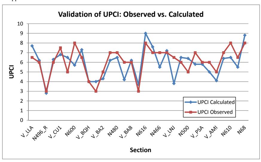
**Figure 5.1 Validation of UPCI Methodology**
#### **5.3 Development of Condition Performance Models**
#### **5.3.1 Selection of a Modelling Method**
The performance of roads over time can be predicted and modelled following deterministic or probabilistic techniques. Deterministic models predict precise condition values based on historical data and observed behaviours. Meanwhile, probabilistic models predict the probability of a future condition subject to the current state and the effects of independent variables affecting roads performance (Karan, 1977). Three different probabilistic approaches have been used in pavement engineering for this purpose: econometric models, Markov Chain models and reliability analysis. Among these, the most widely used technique are the Markov Chains, as they can be easily calibrated, do not require historical databases, can capture non-linear behaviours and are flexible to be adapted when new data is available (Tack, 2005). Markov chains can be used to determine probability transition matrices which reflect the future condition of a road subject to an initial condition state. These matrices can be developed from expert opinion, existing condition data or from evaluations performed in the field during representative time periods.
Markov chain models were selected in this study to define condition performance models for unpaved roads.
#### **5.3.2 Development of Probability Transition Matrices**
Probability transition matrices derived from field evaluations were identified as the most suitable method for this purpose, given the stochastic nature of unpaved roads deterioration and the seasonal variations observed in the field. Data collected in the Chilean road network in three field evaluations were considered. Data was separated in terms of structure strength in two ranges, weak and strong structures. Weak roads presented CBR less than 15%, while strong roads presented CBR equal or greater than 15%. Given the characteristics of the network, all weak roads were earth roads and tracks, while strong roads were gravel roads.
To derive probability transition matrices the following steps were considered:
- Definition of UPCI ranges: Nine states of one UPCI value were defined for the analysis, ranging from 1-1.9 UPCI to 9-10 UPCI.
- Development of a condition summary table: This table presents the total length of roads, in kilometres, changing from an initial condition i to a future condition j during a 6 month period. With this, the condition variations observed per road during two time intervals were captured in the analysis. As presented in Tables 5.2 and 5.3, rows represent the current state i and columns represent the future condition j of the road after a six month period. Only sections that were not rehabilitated during the analysis period were considered for this purpose.
- Definition of Probability Transition Matrices (PTM): Condition summary tables were transformed to probability matrices by estimating the proportion of roads changing from a state i to a state j, given the total road lengths observed per state i. In other words, each tile of Table 5.2 was divided by the total road lengths observed per row.
- Cumulative Probability Transition Matrices: For simulation purposes, cumulative PTM's were defined by summing the cumulative probabilities j per row in each PTM. Two
cumulative PTM's were finally defined, for gravel and earth roads, as presented in Tables 5.4 and 5.5 respectively.
**Table 5.2 Gravel Condition Summary Table**
| | | | | | | Future Condition j (after six months) | | | | | |
|---------------------|-------|------|-------|-------|-------|---------------------------------------|-------|-------|-------|-------|---------|
| | Range | 10-9 | 8.9-8 | 7.9-7 | 6.9-6 | 5.9-5 | 4.9-4 | 3.9-3 | 2.9-2 | 1.9-1 | Total m |
| | 10-9 | 0 | 11000 | 10200 | 11700 | 25600 | 0 | 0 | 0 | 0 | 58500 |
| | 8.9-8 | 0 | 3200 | 0 | 25100 | 5300 | 0 | 0 | 2000 | 0 | 35600 |
| | 7.9-7 | 0 | 0 | 0 | 14200 | 0 | 0 | 0 | 0 | 0 | 14200 |
| Current Condition i | 6.9-6 | 0 | 0 | 0 | 0 | 11700 | 0 | 0 | 0 | 0 | 11700 |
| | 5.9-5 | 0 | 0 | 0 | 0 | 4900 | 0 | 0 | 0 | 0 | 4900 |
| | 4.9-4 | 0 | 0 | 0 | 0 | 0 | 0 | 0 | 0 | 0 | 0 |
| | 3.9-3 | 0 | 0 | 0 | 0 | 0 | 0 | 0 | 3300 | 0 | 3300 |
| | 2.9-2 | 0 | 0 | 0 | 0 | 0 | 0 | 0 | 0 | 0 | 0 |
| | 1.9-1 | 0 | 0 | 0 | 0 | 0 | 0 | 0 | 0 | 0 | 0 |
**Table 5.3 Earth Condition Summary Table**
| | | | | | | Future Condition j (after six months) | | | | | |
|---------------------|-------|------|-------|-------|-------|---------------------------------------|-------|-------|-------|-------|---------|
| | Range | 10-9 | 8.9-8 | 7.9-7 | 6.9-6 | 5.9-5 | 4.9-4 | 3.9-3 | 2.9-2 | 1.9-1 | Total m |
| | 10-9 | 0 | 0 | 2000 | 0 | 0 | 0 | 0 | 0 | 0 | 2000 |
| | 8.9-8 | 0 | 0 | 6800 | 5400 | 0 | 0 | 0 | 0 | 0 | 12200 |
| | 7.9-7 | 0 | 0 | 550 | 1600 | 0 | 400 | 2900 | 0 | 0 | 5450 |
| Current Condition i | 6.9-6 | 0 | 0 | 0 | 1100 | 3000 | 7000 | 5400 | 1400 | 0 | 17900 |
| | 5.9-5 | 0 | 0 | 0 | 3000 | 5900 | 850 | 1700 | 0 | 0 | 11450 |
| | 4.9-4 | 0 | 0 | 0 | 0 | 0 | 0 | 0 | 0 | 0 | 0 |
| | 3.9-3 | 0 | 0 | 0 | 0 | 0 | 0 | 1500 | 0 | 0 | 1500 |
| | 2.9-2 | 0 | 0 | 0 | 0 | 0 | 0 | 0 | 0 | 0 | 0 |
| | 1.9-1 | 0 | 0 | 0 | 0 | 0 | 0 | 0 | 0 | 0 | 0 |
**Table 5.4 Gravel Cumulative Probability Transition Matrix**
| | | | Future Condition j (after six months) | | | | | | | | |
|---------------------|-------|------|---------------------------------------|-------|-------|-------|-------|-------|-------|-------|--|
| | Range | 10-9 | 8.9-8 | 7.9-7 | 6.9-6 | 5.9-5 | 4.9-4 | 3.9-3 | 2.9-2 | 1.9-1 | |
| | 10-9 | 0.00 | 0.19 | 0.36 | 0.56 | 1.00 | 0.00 | 0.00 | 0.00 | 0.00 | |
| | 8.9-8 | 0.00 | 0.09 | 0.09 | 0.79 | 0.94 | 0.94 | 0.94 | 1.00 | 0.00 | |
| | 7.9-7 | 0.00 | 0.00 | 0.00 | 1.00 | 0.00 | 0.00 | 0.00 | 0.00 | 0.00 | |
| Current Condition i | 6.9-6 | 0.00 | 0.00 | 0.00 | 0.00 | 1.00 | 0.00 | 0.00 | 0.00 | 0.00 | |
| | 5.9-5 | 0.00 | 0.00 | 0.00 | 0.00 | 0.67 | 1.00 | 0.00 | 0.00 | 0.00 | |
| | 4.9-4 | 0.00 | 0.00 | 0.00 | 0.00 | 0.00 | 0.00 | 1.00 | 0.00 | 0.00 | |
| | 3.9-3 | 0.00 | 0.00 | 0.00 | 0.00 | 0.00 | 0.00 | 0.00 | 1.00 | 0.00 | |
| | 2.9-2 | 0.00 | 0.00 | 0.00 | 0.00 | 0.00 | 0.00 | 0.00 | 0.00 | 1.00 | |
| | 1.9-1 | 0.00 | 0.00 | 0.00 | 0.00 | 0.00 | 0.00 | 0.00 | 0.00 | 1.00 | |
**Table 5.5 Earth Cumulative Probability Transition Matrix**
| | | | Future Condition j (after six months) | | | | | | | | | |
|---------------------|--------|-------|---------------------------------------|-------|-------|-------|-------|-------|-------|-------|--|--|
| | Range | 8.9-7 | 8.9-8 | 7.9-7 | 6.9-6 | 5.9-5 | 4.9-4 | 3.9-3 | 2.9-2 | 1.9-1 | | |
| | 10-sep | 0.00 | 0.00 | 1.00 | 0.00 | 0.00 | 0.00 | 0.00 | 0.00 | 0.00 | | |
| | 8.9-8 | 0.00 | 0.00 | 0.56 | 1.00 | 0.00 | 0.00 | 0.00 | 0.00 | 0.00 | | |
| | 7.9-7 | 0.00 | 0.00 | 0.10 | 0.39 | 0.39 | 0.47 | 1.00 | 0.00 | 0.00 | | |
| Current Condition i | 6.9-6 | 0.00 | 0.00 | 0.00 | 0.06 | 0.23 | 0.62 | 0.92 | 1.00 | 0.00 | | |
| | 5.9-5 | 0.00 | 0.00 | 0.00 | 0.26 | 0.78 | 0.85 | 1.00 | 0.00 | 0.00 | | |
| | 4.9-4 | 0.00 | 0.00 | 0.00 | 0.00 | 0.00 | 0.26 | 0.78 | 0.85 | 1.00 | | |
| | 3.9-3 | 0.00 | 0.00 | 0.00 | 0.00 | 0.00 | 0.00 | 0.91 | 1.00 | 0.00 | | |
| | 2.9-2 | 0.00 | 0.00 | 0.00 | 0.00 | 0.00 | 0.00 | 0.00 | 0.91 | 1.00 | | |
| | 1.9-1 | 0.00 | 0.00 | 0.00 | 0.00 | 0.00 | 0.00 | 0.00 | 0.00 | 1.00 | | |
#### **5.3.3 Effects of Climate on Unpaved Roads Performance**
Given that the regions are located in a Mediterranean climate, weather variations observed between seasons can be related to the expected performance for different climates. To capture the effects of climate on roads performance, a separate analysis was made considering data collected after winter and summer, rainy and dry seasons respectively. From the analysis it was observed that roads evaluated after the winter (evaluations performed during September) presented an accelerated deterioration trend compared to those evaluated after summer (evaluations performed in April). From collected data, the mean condition of roads after winter was 18% less than the condition observed after summer. In gravel roads a mean condition of 6.4 was observed after winter and a mean condition of 7.3 after summer. While in earth roads a mean condition of 5.0 was observed after winter and a mean condition of 6.2 after summer. A higher difference between seasons is observed in earth roads with respect to gravel roads (25% higher). This evidences that earth roads are more vulnerable to environmental conditions. The slopes of both deterioration trends were estimated and compared to the overall behaviour observed from the complete dataset, representative of a Mediterranean climate.
From the analysis it was concluded that the deterioration trend observed after the summer is representative to a 75% percentile of the modeled dataset. Given that the season presents mean monthly precipitations less than 20 mm, the deterioration trend can be associated with a dry climate. In the case of evaluations performed after winter, it was observed that the trend is representative to a 25% percentile of the dataset. The region presents mean monthly precipitations above 200 mm, which can be associated to a humid climate. For the overall dataset, a 50% percentile represents the Mediterranean climate of the region, with mean monthly precipitations between 20 and 200 mm.
#### **5.3.4 Simulation of Deterioration Trends**
Final deterioration curves were developed using a Monte Carlo simulation. The simulation was performed separately for gravel and earth roads using the cumulative PTM's presented in Tables 5.4 and 5.5. The simulation was performed considering 10,000 trials, where one trial was defined as a set of 20 random numbers between 0% and 100%. Each random number represents the cumulative probability that a road will be in condition i at a certain point in its lifetime. The simulation starts with a new road presenting a UPCI condition of 10. The condition of that road after a six month period is determined from the first random number in a trial. The number is checked from left to right in the condition range of 10-9 (first row) of the cumulative PTM. The condition of the road after six months of service is the first cumulative percentage which the random number exceeds. The second random number is then checked from left to right in the row representative of the condition obtained from the previous step. This checking is performed for all 20 random numbers until a 10 year analysis period is simulated in a trial.
After the 10,000 trials were simulated, the conditions per trial were linearized per condition range. For example, in the cases where the road condition after four consecutive analysis periods presented the same condition range, the UPCI value trend or slope was considered to be 0.20.
#### **5.3.5 Unpaved Roads Condition Performance Curves**
The final unpaved road condition performance curves obtained from the simulation process for strong structure roads (or gravel) and weak structure roads (or earth) are presented in Figures 5.2 and 5.3. Each graph includes three curves, representing the performance observed under dry, Mediterranean and humid climates. It must be noted that the models were defined considering that no maintenance was performed during the service life of the roads. The developed curves represent the long term behaviour of unpaved roads, being the basis required for a life cycle cost analysis to compare different maintenance strategies. The effects of different maintenance treatments over the roads condition and the application of the models for economic analysis are discussed in subsequent sections.
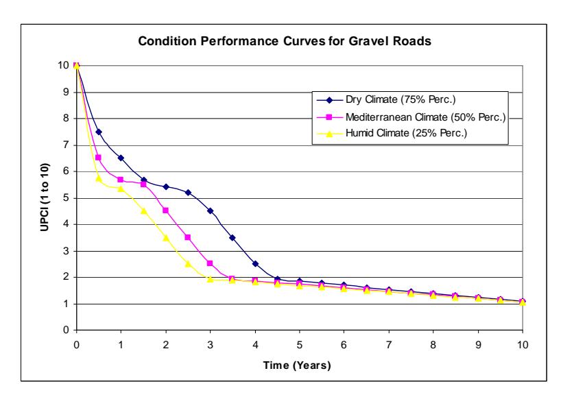
**Figure 5.2 Condition Performance Curves for Strong Structure Roads or Gravel Roads**
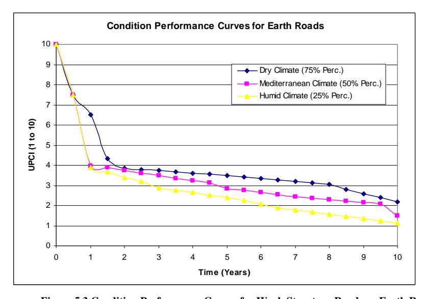
**Figure 5.3 Condition Performance Curves for Weak Structure Roads or Earth Roads**
#### **5.3.6 Analysis of Developed Condition Performance Models**
Both graphs clearly represent the performance observed in the field during the thirteen-month analysis period. As expected for gravel roads, the UPCI value drops significantly during the first year of service due to the appearance of specific distresses caused by traffic and environmental effects. During this phase, functional distresses start to appear, such as corrugations, gravel loss and ravelling. Structural problems may be in an incipient stage, such as slight rutting and pothole formation. This phenomenon coincides with the initial phase of distresses affecting the roads serviceability observed from literature. Then, a stable phase of one to three years is observed while structural and drainage related distresses start to develop. After this stable phase a second accelerated deterioration phase is observed, which characterizes the end of service life of the road. During this phase distresses critically affecting transitability, such as potholes, erosion, drainage problems and significant rutting, are prevalent. These distresses commonly represent the combined effect of structural problems and tend to be collinear. This trend represents the final phase of performance curves observed from literature. In the last five to three years of service, a road presents severe access problems and is in very poor condition, resulting in UPCI values less than 2.
The main difference observed between both graphs is that the condition drops significantly during the first years in the case of earth roads. This is explained by the poor structural capacity of earth roads and absence of a granular wearing course that protects the structure, which tend to deteriorate fast in the presence of traffic and rain. Given this accelerated deterioration, the steady phase is practically reduced to one year, after which a monotonous decreasing trend is observed.
#### **5.4 Maintenance Effects on Roads Condition**
The analysis process for the development of performance curves only considered road sections that were not maintained between two evaluation periods. For sections where maintenance was performed the effects of maintenance on roads condition was analysed. For this, additional data was collected per road including: traffic volumes, type of traffic (considering motorized and non-motorized), traffic distribution (light and heavy), roads with bus service, school bus route and roads requiring ambulance access. Maintenance activities between evaluations were obtained from reports of the local agency. The collected data is summarized in the tables presented in Appendix E.
For the analysis, performance curves were used to estimate the condition of roads on the date they received maintenance. The analysis was done within the six month cycle between maintenance. For the analysis, back calculation of roads condition considering the last evaluation and forward calculation considering the previous evaluation were considered. This was performed for the Mediterranean climate curve as a basis and the climate curve corresponding to the season between evaluations. Table 5.6 is presented as an example to describe the procedure.
The three roads presented in the example were evaluated on September 2008 and April 2009. Between both evaluations the dry season, or summer, prevailed. Between evaluations the dates and types of maintenance were registered, as presented in Table 5.6.
**Table 5.6 Calculation of Maintenance Effects**
| Road
Code | Structure | Traffic UPCI | | Pre
Maintenance
Dry | Pre
Maintenance
Mediterranean | Maintenance | Post
Maintenance
Dry | Post
Maintenance
Med | UPCI |
|--------------|------------------|--------------|-----|---------------------------|-------------------------------------|--------------------------------|----------------------------|----------------------------|------|
| 27 | Earth- Weak | 20 | 3.4 | 3.3 | 3.3 | Local grading
Feb, March/09 | 7.1 | 7.8 | 6.7 |
| 35 | Earth- Weak | 10 | 3.2 | 3.1 | 3.0 | Grading
March/09 | 5.2 | 5.4 | 4.8 |
| 15 | Gravel
Strong | 100 | 6.5 | 6.4 | 6.4 | Grading Oct,
Nov/08 | 5.4 | 5.6 | 4.8 |
Using the performance curves for strong and weak structures, presented in Figures 5.2 and 5.3, the expected UPCI value immediately before the date of the first maintenance was estimated starting with the UPCI value obtained in the first evaluation (September 2008). This value is presented in the "Pre Maint" columns of Table 5.6 for each section. Similarly the expected UPCI value immediately after the maintenance was estimated from UPCI values of the second evaluation (April 2009). For both cases the analysis was done considering the Mediterranean climate and dry climate curves, in order to capture possible fluctuation for different climates. The expected effect or "jump" in the condition caused by a specific maintenance strategy or treatment per climate was calculated as the difference between both UPCI values, pre and post maintenance. In the case where a section was maintained more than once between evaluations, the overall effect was estimated and the date of the first maintenance treatment was considered as a basis.
The analysis was made for all sections that were maintained and considering the effects of the corresponding climates. The results were grouped per maintenance type and climates. The effects were analysed in absolute values and in terms of relative condition improvement, as a percentage of the condition of the road. Descriptive statistics were applied to the results, where sample means, standard deviations, maximum and minimum values were obtained. Results from the analysis are presented in Appendix F.2.
Data statistics were analysed in detail, and Tables 5.7 and 5.8 summarize the final recommendations obtained from the analysis.
**Table 5.7 Maintenance Strategies and UPCI effects Recommended for Gravel Roads**
| | UPCI Increase | Application
Range | | Recommendations |
|-------------------------------------------------------------|---------------|----------------------|-----|---------------------|
| Maintenance Type | | Min | Max | |
| 2 or more Grading (application
subject to traffic level) | 3.2 | 4.0 | 5.5 | Routine Maintenance |
| Local gravel + Grading | 2.7 | 4.0 | 8.5 | Routine Maintenance |
| Culvert/Bridge Repair + Local
Grading | 1.5 | | 5.5 | Rehabilitation |
| Local Gravel | 2.1 | 4.0 | 9.0 | Routine Maintenance |
**Table 5.8 Maintenance Strategies and UPCI effects Recommended for Earth Roads**
| | Application
UPCI
Range
Increase
Min | | | Recommendations |
|--------------------------------|-------------------------------------------------|-----|-----|--------------------------------|
| Maintenance | | | Max | |
| Local Gravel/ Pothole Patching | 2.0 | 5.5 | 10 | Routine Maintenance |
| One Grading | 2.0 | 5.5 | 10 | Routine Maintenance, L Traffic |
| Two Gradings | 3.0 | 5.5 | 10 | Routine Maintenance, M traffic |
| Culvert Repair + One Grading | 3.5 | 4.0 | 5.5 | Rehabilitation L traffic |
| Local gravel + One Grading | 4.0 | 4.0 | 5.5 | Rehabilitation L traffic |
The following findings were obtained from the analysis:
- Four types of maintenance strategies were applied to gravel roads and five types of maintenance strategies to earth roads. Based on the effects on roads condition and literature, recommendations were made for their classification and development of maintenance standards.
- A variability of 30% in average was observed on the standard deviation of calculated UPCI increases. This trend was observed in gravel and earth roads.
- Most variable observations were obtained for one grading in earth roads, where variability of the standard deviation was more than 50%. This is explained by the fact that the effectiveness of one grading is very sensitive to the condition of the road prior application, especially when a light blading is considered. Given its variable effectiveness and reduced contribution to increase UPCI after application, simple light grading is recommended as a minimum strategy for low and medium volume traffics in earth roads and for low traffic volumes on gravel roads.
- Strategies that combined more than one maintenance treatment or considered more than one application of a specific maintenance treatment within the analysed period, presented higher effectiveness and low variability. For example, the application of two grading in earth roads presented a variability of 15% in terms of its standard deviation. This value is considerably less than the 50% or more observed for one grading application.
- Ranges of UPCI were obtained from the analysis of maximum and minimum values for each strategy. This resulted in recommendations of trigger values for the design of maintenance standards for routine maintenance, rehabilitation and reconstruction.
- The effectiveness of strategies was highly dependent on traffic volumes. It was therefore essential to consider maintenance policies for different traffic volumes. Different application frequencies should be defined in terms of vehicles per day. In this sense, the analysed data was consistent with literature recommendations.
- A relationship between maintenance effectiveness and climate was not apparent from the analysis. This could be explained by the fact the calculation of UPCI considered the developed condition models, which already capture the effects of climate. Considering this, the effects of climates should be accounted for as a long term performance effect and not as a maintenance strategy effect, to avoid double counting.
# **5.5 Validation of Unpaved Roads Condition Performance Models and Maintenance Recommendations**
The validation of performance models and maintenance effects considered data collected in the third and fourth field evaluations of the Chilean road network. The analysis consisted on the comparison of UPCI values from the fourth field evaluation contrasted to predicted UPCI values considering the third field evaluation. For this, performance curves were used to calculate the expected condition (calculated UPCI) of roads after a 24 month period and considering the maintenance activities performed per road during that period. The expected condition (calculated UPCI) was plotted and compared to the observed condition obtained from field evaluations (observed UPCI). Calculated and observed UPCI values for earth and gravel roads are presented in Figure 5.4 and 5.5. Both samples were statistically compared with a 95% confidence following the t test for difference in means. From the analysis performance models for earth and gravel roads and the effects of maintenance on roads condition were successfully validated. A trend is observed in both graphs where observed data tend to be higher than calculated values when UPCI is more than 6. This is explained by the fact that maximum UPCI values were established for each maintenance strategy, given that in the practice a lower effectiveness is observed for routine maintenance and rehabilitation for roads in good condition. With this, calculated UPCI is conservative when compared to the performance observed in the field for higher UPCI values. The statistic test and data considered in the analysis is presented in Appendix F.3.
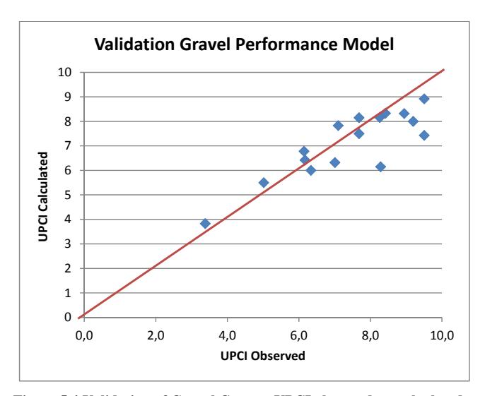
**Figure 5.4 Validation of Gravel Curves: UPCI observed vs. calculated**

**Figure 5.5 Validation of Earth Curves: UPCI observed vs. calculated**
#### **5.6 Summary of the Chapter**
The basis for condition performance analysis and prediction in the long term considered in the proposed management system is presented in detail in the present chapter. The network evaluation methodology recommended, the UnPaved Roads Condition Index (UPCI), was successfully validated. With this, the unpaved roads condition performance models were developed based on a reliable evaluation method.
Performance models were obtained from the statistical analysis of the road deterioration observed in a thirteen month period. The modelling technique selected was Markov chain models, which can reliably predict the stochastic nature and non-linear performance of unpaved roads over time. Performance curves for strong structures or gravel roads and weak structures or earth roads were finally obtained from Monte Carlo simulation. Data that was not considered in the development of performance curves was analysed in detail to define maintenance recommendations. Maintenance effects on roads condition were obtained from the analysis; in addition, trigger values for different maintenance strategies were defined.
The unpaved roads condition performance models and effect of maintenance on roads condition were validated. For this, data was collected in October 2011 and compared to data collected 24 months before but projected to the same timeframe with the use of performance models. From the analysis, condition performance models and maintenance recommendations were successfully validated. The four elements developed and validated in the present Chapter, UPCI methodology, performance curves and maintenance recommendations are the core elements forming the Condition Performance Module.
# **Chapter 6**
# **Development of the Network Maintenance Module**
#### **6.1 Introduction**
After analysing the current condition of a road network, the next step in the management process is to decide how to maintain roads in order to achieve a desired network standard. For this, the proposed management system considers the development of the Network Maintenance Module, which includes all required elements for short and long- term maintenance decisions.
To decide upon the most suitable maintenance strategy for a specific road, rational comparisons about long term performance and related maintenance costs should be considered. The costeffectiveness analysis method was considered for this purpose, as it objectively estimates the effects of roads condition and maintenance during the whole life cycle of a road.
Optimal maintenance standards were developed considering eighteen scenarios at four different budget levels. Scenarios considered two types of road structure, three climate zones and three traffic levels. For each scenario, two maintenance standards were defined, considering two different routine maintenance policies. From the cost-effectiveness analysis, optimal standards were recommended and the optimum budget level was defined for each scenario.
#### **6.2 Development of Maintenance Strategies**
#### **6.2.1 Definitions**
Maintenance treatments refer to the application of a specific maintenance treatment to the road surface. The effectiveness of treatments vary depending on the level of deterioration prior application, material properties, traffic and the activities considered in the treatment (such as prior compaction, reshaping, forming, etc.). Most common maintenance treatments for unpaved roads were described in detail in Chapter 2. These could be summarized in four main treatment categories:
- Drainage Maintenance and Improvement (D): including maintenance of subdrains and drains, ditch improvement and culvert replacement.
- Blading or Grading (B): which could be performed as dry blading, wet blading, light blading and heavy blading/grading. In addition the effectiveness of the blading can be improved in the presence of certain defects when considering reshaping reworking and forming.
- Local or Spot Gravelling (R): gravelling of short sections on a road, typically only on curves, steep gradients, potholes or isolated rock outcrops.
- Gravelling (G): defined as the addition of a suitable wearing course layer of unbound gravel, typically 100 mm to 150 mm in thickness over the entire length of the improved section.
Some maintenance treatments can be applied for the upgrade of a road to a higher surface standard. This is the case when earth roads are gravelled and improved to a gravel standard or when a seal is applied to an earth or gravel road. The discussion on the present research centres on the application of maintenance treatments to improve the condition of roads and surface upgrades from earth to gravel roads for high traffic volumes. The approach, also detects candidate roads for surface upgrades from earth or gravel to surface treatment or pavement when a maximum traffic volume is reached.
Depending on the type of deterioration and condition of an unpaved road, treatments can be combined and grouped in three main types:
- Routine maintenance, which is applied on a proactive programmed basis when roads present incipient deterioration to extend a good performance over time.
- Rehabilitation, which combines reactive policies to improve the condition of a road in an advanced deterioration phase.
- Reconstruction or Emergency Maintenance, which is commonly applied in unpaved roads presenting excessive damage or wear, commonly related to severe drainage problems or abnormal use of the road.
In the present research the terms routine maintenance, rehabilitation and reconstruction will be used. In addition a fourth category was considered as minimum routine maintenance, required to warranty basic access in rural areas.
Maintenance strategies can be defined as all treatments undertaken to maintain and provide serviceable roads over their life cycle. Strategies may combine several treatments to improve specific functional and structural problems of a road. Agencies usually define strategies based on previous experiences, subject to available technologies and funding. Maintenance strategies should consider routine maintenance, rehabilitation and reconstruction to ensure a suitable condition level of roads throughout their service life.
#### **6.2.2 Effects of Traffic on Maintenance**
Several studies have evaluated the impact of traffic volumes on the effectiveness of certain maintenance treatments (Provencher, 1995; Visser, 1981; Kerali, 1991). In particular, during the development of HDM III models, the effects of blading frequency on roughness progression and gravel loss were studied in detail. From the study it was evidenced that a long term average roughness level is reached when a constant blading frequency is considered for a certain traffic volume. When the traffic decreases or the blading frequency increases the average roughness decreases and the long term average value advances in time. From economic analysis, the study concluded that a blading policy at intervals of 4,000 vehicles is close to optimal (Paterson, 1991).
Regarding traffic loads, studies have evidenced that no significant differences in the modeling of gravel loss and riding quality deterioration of rural gravel roads were found by separating the traffic into light and heavy vehicles. Moreover, travelling speeds may affect significantly the progression of roads deterioration, especially in the presence of dry conditions and independently, if light or heavy traffic is considered (NITRR, 2009).
In light of these recommendations and findings obtained from field evaluations, it was decided to consider different maintenance strategies for three traffic volumes. The estimation was made considering the recommendation of optimal frequencies suggested by Paterson (1991), for intervals of 4,000 vehicles.
#### **6.2.3 Proposed Maintenance Strategies**
Four budget levels were considered in the definition of maintenance strategies: Minimum (B1), Low (B2), Medium (B3) and High (B4).Taking into account that suitable maintenance equipment and funding may vary significantly between agencies in charge of rural roads in developing countries, budget levels were defined in terms of the quality of applied maintenance. This was concluded after reviewing the current state-of-the-practice, available literature and from field evaluations, where the effectiveness of treatments applied in unpaved roads significantly depend on available labour, materials and equipment. Frequency of treatment application is most common and usually programmed in terms of traffic volumes (Lebo, 2000; Paterson, 1991). Given this, budget levels were defined in terms of quality and how extensively maintenance treatments are applied as presented in Table 6.1. Names given to each treatment, budget level and combination of both are presented in parenthesis in the table.
**Table 6.1 Maintenance Treatments per Funding Levels**
| Maintenance
Treatment | Minimum Budget
(B1) | Low Budget (B2) | Medium Budget (B3) | High Budget (B4) |
|----------------------------------------------------|--------------------------------------------------------------------------------|--------------------------------------------------------------------------------|---------------------------------------------------------------------------------|--------------------------------------------------------------------------------------------------------|
| Drainage
Improvement/Culvert
Replacement (D) | 1 per 8 km, 10m long
(DB2) | 1 per 8 km, 10m long
(DB2) | 1 per 6 km, 10m long
(DB3) | 1 per 4 km, 10m long (DB4) |
| Grading (B) | Sporadic light blading
to ensure minimum
access (BB1) | light blading (BB2) | heavy blading or
grading with localized
compaction when
required (BB3) | heavy blading with
reshaping, forming and
compaction when required
(BB4) |
| Local Gravel/
Pothole Patching (R) | 5m3
per km (50
potholes/km of
1mx1mx10cm) (RB2) | 5m3
per km (50
potholes/km of
1mx1mx10cm) (RB2) | 8m3
per km (80
potholes/km of
1mx1mx10cm) (RB3) | 12m3 per km (120
potholes/km of
1mx1mx10cm) (RB4) |
| Gravelling (G) | 50mm layer, 7m wide
road, light blading for
surface preparation
(GB2) | 50mm layer, 7m wide
road, light blading for
surface preparation
(GB2) | 100mm layer, 7m wide
road, heavy blading for
surface preparation
(GB3) | 150mm layer, 7m wide
road, heavy blading,
reshaping and forming for
surface preparation (GB4) |
In addition to budget and traffic scenarios, it was observed from the practice that routine maintenance was applied combining local gravel and minimum grading (RM1) or as a routine grading (RM2). The effects on roads condition for both approaches were captured on field evaluations. A minimum maintenance strategy (RMin) was also defined considering minimum blading criteria for routine maintenance, where only sporadic light blading is applied. This is considered as a minimum routine maintenance warranting basic access in rural areas.
The three strategies were defined in terms of three traffic volumes: Low (LT), Moderate (MT) and High (HT). With this, nine strategies were defined per budget scenario for gravel and earth roads, considering different traffic and routine maintenance approaches, as presented in Tables 6.2 and 6.3.
**Table 6.2 Maintenance Strategies for Gravel Roads**
| Strategy | Low Traffic-LT (<100 AADT) | Moderate Traffic-MT
(100-200 AADT) | High Traffic-HT (>200 AADT) |
|------------|----------------------------|---------------------------------------|-----------------------------|
| Gravel | GRMin-LT | GRMin -MT | GRMin -HT |
| Minimum | Minimum: 2MinB/year | Minimum: 6MinB/year | Minimum: 10MinB/year |
| Strategy | Rehabilitation: 2B+10%G | Rehabilitation: 6B+25%G | Rehabilitation: 12B+40%G |
| (GRMin) | Reconstruction: 2B+30%G+C | Reconstruction: 6B+75%G+C | Reconstruction: 12B+100%G+C |
| Gravel | GRM1-LT | GRM1-MT | GRM1-HT |
| PM | Routine 1: 2BLB+2R/year | Routine 1: 6BLB+6R/year | Routine 1: 10BLB+10R/year |
| Strategy 1 | Rehabilitation: 2B+10%G | Rehabilitation: 6B+25%G | Rehabilitation: 12B+40%G |
| (GRM1) | Reconstruction: 2B+30%G+C | Reconstruction: 6B+75%G+C | Reconstruction: 12B+100%G+C |
| Gravel | GRM2-LT | GRM2-MT | GRM2-HT |
| PM | Routine 2: 4B | Routine 2: 12B | Routine 2: 20B |
| Strategy 2 | Rehabilitation: 2B+10%G | Rehabilitation: 6B+25%G | Rehabilitation: 12B+40%G |
| (GRM2) | Reconstruction: 2B+30%G+C | Reconstruction: 6B+75%G+C | Reconstruction: 12B+100%G+C |
**Table 6.3 Maintenance Strategies for Earth Roads**
| Strategy | Low Traffic (<50 AADT) | Moderate Traffic (AADT 50-100) | High Traffic (100> AADT) |
|------------|---------------------------|--------------------------------|-----------------------------|
| Earth | ERMin-LT | ERMin -MT | ERMin -HT |
| Minimum | Minimum: 2MinB/year | Minimum: 6MinB/year | Minimum: 10MinB/year |
| Strategy | Rehabilitation: 2B+10%G | Rehabilitation: 6B+25%G | Rehabilitation: 12B+40%G |
| (ERMin) | Reconstruction: 2B+30%G+C | Reconstruction: 6B+75%G+C | Reconstruction: 12B+100%G+C |
| | ERM1-LT | ERM1 -MT | ERM1 -HT |
| Earth | Routine 1: 1BLB+1R/year | Routine 1: 4BLB+4R/year | Routine 1: 6BLB+6R/year |
| Strategy 1 | Rehabilitation: 2B+2R | Rehabilitation: 6B+6R | Rehabilitation: 12B+12R |
| (ERM1) | Reconstruction: 2B+2R+C | Reconstruction: 6B+6R+C | Reconstruction: 12B+12R+C |
| | ERM2-LT | ERM2 -MT | ERM2 -HT |
| Earth | Routine 2: 2B | Routine 2: 6B | Routine 2: 12B |
| Strategy 2 | Rehabilitation: 2B+2R | Rehabilitation: 6B+6R | Rehabilitation: 12B+12R |
| (ERM2) | Reconstruction: 2B+2R+C | Reconstruction: 6B+6R+C | Reconstruction: 12B+12R+C |
Regarding budget levels, the minimum maintenance strategy was only defined for the minimum budget level, while the other two strategies were estimated for Low, Medium and High Budget. From this, 21 scenarios were considered in the analysis for each road type, totaling in 42 scenarios (3\*ERMin+9\*ERM1+9\*ERM2 for earth and 3\*GRMin+9\*GRM1+9\*GRM2 for gravel). The type of treatment applied in each scenario varies depending on the budget level considered.
#### **6.2.4 Maintenance Costs**
Maintenance costs were estimated for each scenario considering unit prices specified in 2007 by the Ministry of Public Works of Chile (MOP, 2007) for maintenance performed by the agency. These prices were corrected to the present by considering the annual consumer price index (IPC) recommended by the Central Bank of Chile for each year (INE, 2011). Unit prices per treatment are presented in Table 6.4. Prices defined by the MOP are provided in terms of materials and occasional replacement of equipment parts. Detailed estimation of treatment costs per budget level are presented in Appendix C.
**Table 6.4 Maintenance Treatment Costs**
| Maintenance Treatment | UNIT | CAD\$ |
|--------------------------------|------|--------|
| Local Gravel/ Pothole Patching | m³ | 15.58 |
| Light Blading | km | 89.79 |
| Culvert Replacement | m | 296.49 |
| Gravel Application | m³ | 22.69 |
Upgrade treatments and costs were also estimated from the available literature. These are special projects for improving the surface standard from earth to gravel, and from gravel to surfacing or double treatment. These should be evaluated under a project level analysis, recommended when high traffic levels justify upgrading the roads surfacing. Upgrade costs are presented in Appendix C.4.
### **6.3 Development of Optimal Maintenance Standards**
#### **6.3.1 Definition of Maintenance Standards**
Maintenance policies should consider the application of treatments within suitable service levels, subject to the effects of each treatment on the functional and structural condition of roads. Maintenance standards can be defined as maintenance strategies where threshold values are defined for the application of the different types of treatments considered. Standards may vary depending on agencies strategic policies, such as desired service level of the network, access and mobility standards, type of network, among others.
From developed curves, which are presented in Figures 5.2 and 5.3, three deterioration stages were identified for earth and gravel roads, as discussed in section 5.3.6. The type of maintenance considered during the life cycle of a road should be defined in terms of the deterioration types and severities observed. It is expected that routine maintenance should be applied at the first deterioration stage, where UPCI values drop due to the appearance of functional related deteriorations such as gravel loss, corrugations and raveling. Rehabilitation should be considered in a second stage of deterioration, where structural problems start to appear, such as rutting and pothole formation. Rehabilitation should be applied as a corrective policy to avoid severe structural deterioration that may cause impassability. Finally, reconstruction or emergency maintenance should be applied in those sections presenting accessibility problems caused by severe structural problems such as deep potholes, rutting and erosion.
Threshold levels for each maintenance type were defined considering the three deterioration phases discussed previously. UPCI trigger values were first obtained from the statistical analysis of maintenance applications, considering maximum and minimum application values and treatments effects on roads condition, as presented in Chapter 5. These were then contrasted to trends observed in performance curves (Figures 5.2 and 5.3), and adjusted accordingly. Finally, threshold levels for routine maintenance, rehabilitation and reconstruction were defined. Performance "jump" values were defined per treatment type and budget levels, subject to the quality and effectiveness of each maintenance treatments. Recommended application ranges per strategy considering threshold values and performance "jump" values per budget level are presented in Table 6.5 and 6.6, for gravel and earth roads respectively.
**Table 6.5 Application Ranges and Performance Jump Values for Gravel Roads**
| | | | | UPCI Jump Values per Budget Level | |
|------------------------------------------|------------------------------|---------|-----|-----------------------------------|------|
| Maintenance type | Application Ranges
(UPCI) | Minimum | Low | Medium | High |
| RMin: Minimum Routine | 10-4 | 1.0 | | | |
| RM1: Local Gravel and
Minimum Grading | 10-5.5 | | 1.5 | 2.5 | 3.0 |
| RM2: Routine Grading | 10-5.5 | | 2.5 | 3.5 | 4.0 |
| Rehabilitation | 4-5.5 | 4.0 | 4.0 | 5.0 | 5.5 |
| Reconstruction | <4 | 5.0 | 5.0 | 6.0 | 6.5 |
**Table 6.6 Application Ranges and Performance Jump Values for Earth Roads**
| | | | | UPCI Jump Values per Budget Level | |
|------------------------------------------|------------------------------|---------|-----|-----------------------------------|------|
| Maintenance type | Application Ranges
(UPCI) | Minimum | Low | Medium | High |
| RMin: Minimum Routine | 10-4 | 1.0 | | | |
| RM1: Local Gravel and
Minimum Grading | 10-5 | | 1.5 | 2.5 | 3.0 |
| RM2: Routine Grading | 10-5 | | 2.5 | 3.5 | 4.0 |
| Rehabilitation | 4-5 | 3.5 | 3.5 | 4.5 | 5.0 |
| Reconstruction | <4 | 5.0 | 5.0 | 5.75 | 6.25 |
When a road is in a relatively good condition prior to the need for maintenance, the maximum condition level achieved will depend on the type of treatment considered. It is commonly observed, for example, that the application of routine maintenance does not warranty a maximum condition equivalent to a new road. This trend is observed in paved and unpaved roads, and has been considered by most models and management systems (Paterson, 1991; Kerali, 1991; Kerali, 2000; Provencher, 1995). Maximum condition levels achieved by maintenance strategies have been defined for the study, based on the analysis of condition and maintenance data. Table 6.7 presents maximum values considered per strategy for gravel and earth roads.
**Table 6.7 Maximum Condition Levels per Strategy**
Final considerations regarding the effectiveness of minimum and routine maintenance are their effectiveness over time after successive treatment applications. In particular, studies have demonstrated that when a constant blading frequency is considered for a certain traffic volume, a long term average roughness level is reached. During the development of HDM performance models, Paterson (1991) demonstrated that the effectiveness of blading decreases until this average level is reached. These findings were proved in the field, where it was observed that the effectiveness of blading decreased when no other treatment was considered. Given this, it was considered that for the analysis of minimum and routine maintenance their effectiveness in terms of UPCI "jump" was reduced in 5% starting from the second application when no rehabilitation was considered. The 5% was considered as a realistic approach for a 10 year analysis period (20 semi-annual cycles), where the successive applications of routine maintenance would be ineffective if no rehabilitation is performed to improve roads structure and drainage.
### **6.3.2 Cost-Effectiveness Analysis of Proposed Maintenance Standards**
Cost effectiveness is calculated as effectiveness divided by the life-cycle cost of each strategy. Effectiveness can be defined as the area under the performance curve and above a minimum service level, which is weighted by section length and traffic (Haas, 1994; Wei, 2004). This area can be interpreted as the benefits of road users given the performance of a road in the long term. A minimum service level for rural roads can be defined as the minimum condition that ensures all-weather access. From available data and analysis of developed performance curves (Figures 5.2 and 5.3), this is observed for UPCI values above 4. Below this level of service roads require reconstruction or emergency maintenance. Effectiveness is estimated considering the following formula:
$$\begin{split} \textit{Effectiveness} &= \left\{ \sum_{\textit{Treat.Semi-Year}}^{\textit{UPCI}_T \geq \textit{UPCI}_M} (\textit{UPCI}_T - \textit{UPCI}_M) - \left( \sum_{\textit{UPCI}_N \geq \textit{UPCI}_M}^{\textit{Treat.Semi-Year}} (\textit{UPCI}_M - \textit{UPCI}_N) \right) \right\} \times \textit{AADT} \\ &\times \textit{Length of Section} \end{split}$$
(6)
#### Where:
UPCIT = UnPaved Road Condition Index (UPCI) after treatment for each year until UPCI minimum is reached;
UPCIM = minimum acceptable condition level (UPCI<4);
UPCIN = yearly UPCI from the needs year to the treatment year;
AADT = annual average daily traffic; and
Length of section = road length.
Given that the comparison between maintenance strategies was performed under the same basis, considering 1 km of road and under the same traffic condition, the last term of Equation 6 can be eliminated. In addition, the analysis considered a semi-annual period given the climate seasonal effects on roads deterioration, therefore, the areas per period were estimated as the mean values observed within a six-month cycle. The minimum acceptable UPCI value was considered as 4. With this, effectiveness calculation was estimated in terms of unit effectiveness and the formula was simplified as follows:
Unit Effectiveness =
$$\left\{\sum_{n=1}^{20} \left(\frac{(UPCI_B + UPCI_A)}{2}\right) - 4 \times 20\right\}$$
(7)
Where:
n= Semi-annual cycle of six months for a 10 year analysis period (n= 1, 2, 3…20);
UPCIB = Condition immediately before applying a treatment;
UPCIA = Condition immediately after applying a treatment.
Effectiveness calculations for each maintenance strategy considering three different climates are presented in Appendix G.1 and G.2 for gravel and earth roads respectively.
For the calculation of the life-cycle costs of each strategy, the present worth of costs was considered (PWC). The discount rate defined for the analysis was 8%, based on the practice of the MOP and recommendations from agencies in developing countries (Almonte, 2001; Mideplan, 2004). Present worth of costs was calculated considering all treatments applied within the life cycle of a road under each specific strategy. A life cycle analysis period of 10 years and a semi-annual basis was considered. Equation 8 presents the formula considered.
$$PWC = \sum_{n=1}^{20} \frac{1}{(1+i)^n} \times Treatment \ cost \ (n)$$
(8)
Where:
PWC = Present worth of costs;
n= Semi-annual cycle of six months for a 10 year analysis period (n= 1, 2, 3…20);
i = Discount rate, 8%;
Treatment cost (n) = Costs of treatments considered in the strategy applied in cycle n
Having the Effectiveness and PWC for each strategy Cost Effectiveness (CE) was calculated following Equation 9, as recommended by the literature (TAC, 1997; Haas; 1994)
$$CE = Effectiveness/PWC$$
(9)
Cost Effectiveness of the three maintenance strategies (RMin, RM1 and RM2) were calculated for all scenarios included in the experiment factorial, considering: four budget scenarios (minimum, low, medium and high), three traffic levels (low, moderate, high), two types of structures (earth and gravel) and three climates (dry, Mediterranean, humid). From the comparison between budget levels, unfeasible scenarios, where PWC of minimum budgets were higher than low budgets, were detected and eliminated from the analysis. Results are presented in Appendix G3 and G4, for gravel and earth roads respectively. Unfeasible scenarios were observed only in earth roads, where minimum maintenance caused access problems (UPCI < 4), which required the application of several reconstructions during the whole life cycle. These cases are marked in red in the tables presented in Appendix G.4.
#### **6.3.3 Optimal Maintenance Standards**
Marginal Cost Effectiveness (MCE) is defined as a heuristic technique used to obtain near optimal maintenance standards for specific conditions. The cost effectiveness analysis method was used to compare the different strategies defined per scenario (Haas, 1994). This method has been largely used by several agencies to as a basis for priority programming.
MCE is calculated as the ratio obtained from dividing the difference between the effectiveness of a basis strategy (Ebasis) minus the effectiveness of an alternative strategy (Ealt), divided by the difference of the PWC of the basis (PWCbasis) minus the PWC of the alternative (PWCalt). This is presented in Equation 10.
$$MCE = (E_{basis}-E_{alt})/(PWC_{basis}-PWC_{alt})$$
(10)
The most cost effective strategy is selected from the analysis. If MCE is negative or if the effectiveness of the alternative is less than the basis, then the basis strategy is selected.
The MCE analysis was considered to identify which strategy was more cost-effective for the low, medium and high budget levels. Given that the minimum strategy is only considered as a basis at a minimum funding level, strategies RM1 and RM2 were included in the analysis. Tables 6.8 and 6.9 present a summary of the MCE analysis and selected strategies per scenario for gravel and earth roads.
**Table 6.8 MCE Analysis for Gravel Roads**
| | | | Dry Climate | | | Mediterranean Climate | | Humid Climate | | |
|----------------------|----------------------|---------|-------------|----------|----------|-----------------------|----------|---------------|---------|----------|
| | Budget
Level | Low | Medium | High | Low | Medium | High | Low | Medium | High |
| Traffic | | | | | | | | | | |
| Low (<100
AADT) | Selected
Strategy | GRM2 | GRM2 | GRM1 | GRM1 | GRM2 | GRM1 | GRM1 | GRM2 | GRM1 |
| | MCE | 0.0005 | 0.0003 | -0.00004 | -0.0001 | 0.0002 | -0.0001 | -0.0005 | 0.0001 | -0.0001 |
| Moderate
(100-200 | Selected
Strategy | GRM2 | GRM2 | GRM1 | GRM1 | GRM2 | GRM1 | GRM1 | GRM2 | GRM1 |
| AADT) | MCE | 0.0001 | 0.00006 | -0.00001 | -0.00003 | 0.00003 | -0.00002 | -0.00011 | 0.00002 | -0.00002 |
| High
(>200 | Selected
Strategy | GRM2 | GRM2 | GRM1 | GRM1 | GRM1 | GRM1 | GRM1 | GRM2 | GRM1 |
| AADT) | MCE | 0.00007 | 0.00005 | -0.00001 | -0.00002 | 0.00003 | -0.00001 | -0.00008 | 0.00001 | -0.00001 |
**Table 6.9 MCE Analysis for Earth Roads**
| | | Dry Climate | | | | Mediterranean Climate | | | Humid Climate | | |
|------------------------|----------------------|-------------|---------|----------|---------|-----------------------|----------|---------|---------------|----------|--|
| | Budget
Level | Low | Medium | High | Low | Medium | High | Low | Medium | High | |
| Traffic | | | | | | | | | | | |
| Low (<50
AADT) | Selected
Strategy | ERM2 | ERM1 | ERM2 | ERM2 | ERM2 | ERM1 | ERM2 | ERM2 | ERM1 | |
| | MCE | -0.002 | -0.001 | -0.001 | -0.002 | -0.004 | -0.001 | -0.002 | -0.004 | -0.001 | |
| Moderate
(50-100 | Selected
Strategy | ERM2 | ERM2 | ERM2 | ERM2 | ERM2 | ERM2 | ERM2 | ERM2 | ERM2 | |
| AADT) | MCE | -0.0003 | -0.0001 | -0.00005 | -0.0004 | -0.0005 | -0.0002 | -0.0004 | -0.0005 | -0.0002 | |
| High
(>100
AADT) | Selected
Strategy | ERM2 | ERM1 | ERM1 | ERM1 | ERM1 | ERM1 | ERM2 | ERM2 | ERM1 | |
| | MCE | 0.0004 | -0.0001 | -0.00002 | -0.0004 | -0.0003 | -0.00007 | -0.0004 | -0.0004 | -0.00007 | |
From the analysis it was observed that some MCE values were positive, given by higher effectiveness of the basis and lower costs of the alternative. In these cases, the selection of either the most effective or less expensive alternative relies on the road manager. In this research, the alternative presenting the highest effectiveness was selected as the optimal, therefore the basis strategy was defined as the optimal. It was also observed that some MCE values were negative, given by lower effectiveness of the basis and lower costs of the alternative. In these cases, the alternative presented highest effectiveness and was therefore selected as the optimal.
Optimum budget levels were identified from the comparison of cost effectiveness for all budget levels per scenario. From this it was concluded that for gravel roads the optimum funding level for dry climate was the minimum budget and for Mediterranean and humid climates was the low budget. For earth roads the optimum budget level for dry climate was the minimum budget and for Mediterranean and humid climates was the medium budget. Unfeasible minimum funding scenarios in earth roads were observed in Mediterranean and humid climates under low and moderate traffic levels.
Given that traffic volumes are considered in the analysis in terms of AADT, it is recommended that for high volumes of heavy traffic (commonly greater than 20%) the optimal standards for the immediately higher level of traffic be considered. This could be adopted, for example, for seasonal variations on heavy traffic volumes due to harvesting or forestry production. For example, if a gravel road presents low volume traffic of 50 AADT where 30% of the total traffic is trucks, it is recommended to consider maintenance standards for a moderate traffic level.
A summary of the results obtained from the cost-effectiveness analysis is presented in Tables 6.10 and 6.11. Optimum recommended standards per climate and traffic are coloured in light grey in the tables and unfeasible scenarios minimum budget scenarios in earth roads are coloured in dark grey.
**Table 6.10 Optimum Standards for Gravel Roads**
| | | | | Dry Climate | | | | Mediterranean Climate | | | | Humid Climate | |
|-----------------------------|---------------------|---------------|---------------|----------------|----------------|---------------|---------------|-----------------------|----------------|---------------|---------------|----------------|----------------|
| Traffic | Analysis | Min
Budget | Low
Budget | Med.
Budget | High
Budget | Min
Budget | Low
Budget | Med.
Budget | High
Budget | Min
Budget | Low
Budget | Med.
Budget | High
Budget |
| | Optimal
Strategy | GRMin | GRM2 | GRM2 | GRM1 | GRMin | GRM1 | GRM2 | GRM1 | GRMin | GRM1 | GRM2 | GRM1 |
| Low | Mean
UPCI | 6.40 | 7.16 | 7.74 | 7.67 | 6.13 | 6.24 | 7.02 | 6.86 | 6.06 | 6.17 | 6.64 | 6.49 |
| Traffic
(<100
AADT) | Unit
Effect. | 48 | 63 | 75 | 73 | 43 | 125 | 140 | 137 | 41 | 123 | 133 | 130 |
| | PWC
CAD\$ | 1556 | 2359 | 3538 | 5994 | 1556 | 2203 | 3538 | 5994 | 1603 | 2203 | 3538 | 5994 |
| | CE | 0.031 | 0.027 | 0.021 | 0.012 | 0.027 | 0.057 | 0.040 | 0.023 | 0.026 | 0.056 | 0.038 | 0.022 |
| | Optimal
Strategy | GRMin | GRM2 | GRM2 | GRM1 | GRMin | GRM1 | GRM2 | GRM1 | GRMin | GRM1 | GRM2 | GRM1 |
| | Mean
UPCI | 6.40 | 7.16 | 7.74 | 7.67 | 6.13 | 6.24 | 7.02 | 6.86 | 6.06 | 6.17 | 6.64 | 6.49 |
| Mod.
Traffic
(100-200 | Unit
Effect. | 48 | 63 | 75 | 73 | 43 | 125 | 140 | 137 | 41 | 123 | 133 | 130 |
| AADT) | PWC
CAD\$ | 4480 | 7076 | 10614 | 17982 | 4480 | 6608 | 10614 | 17982 | 4598 | 6608 | 10614 | 17982 |
| | CE | 0.011 | 0.009 | 0.007 | 0.004 | 0.009 | 0.019 | 0.013 | 0.008 | 0.009 | 0.019 | 0.013 | 0.007 |
| | Optimal
Strategy | GRMin | GRM2 | GRM2 | GRM1 | GRMin | GRM1 | GRM1 | GRM1 | GRMin | GRM1 | GRM2 | GRM1 |
| High | Mean
UPCI | 6.40 | 7.16 | 7.74 | 7.67 | 6.13 | 6.24 | 6.65 | 6.86 | 6.06 | 6.17 | 6.64 | 6.49 |
| Traffic
(>200
AADT) | Unit
Effect. | 48 | 63 | 75 | 73 | 43 | 125 | 133 | 137 | 41 | 123 | 133 | 130 |
| | PWC
CAD\$ | 7404 | 11793 | 17689 | 29971 | 7404 | 11014 | 17032 | 29971 | 7592 | 11014 | 17689 | 29971 |
| | CE | 0.89 | 0.73 | 0.58 | 0.33 | 0.78 | 1.55 | 1.07 | 0.63 | 0.74 | 1.53 | 1.03 | 0.59 |
**Table 6.11 Optimum Standards for Earth Roads**
| | | | | Dry Climate | | | | Mediterranean Climate | | | | Humid Climate | |
|---------------------------|---------------------|---------------|---------------|----------------|----------------|---------------|---------------|-----------------------|----------------|---------------|---------------|----------------|----------------|
| Traffic | Analysis | Min
Budget | Low
Budget | Med.
Budget | High
Budget | Min
Budget | Low
Budget | Med.
Budget | High
Budget | Min
Budget | Low
Budget | Med.
Budget | High
Budget |
| | Optimal
Strategy | ERMin | ERM2 | ERM1 | ERM2 | ERMin | ERM2 | ERM2 | ERM1 | ERMin | ERM2 | ERM2 | ERM1 |
| Low Traffic | Mean
UPCI | 6.97 | 7.46 | 7.84 | 8.01 | 6.57 | 7.00 | 7.81 | 7.92 | 6.53 | 6.87 | 7.78 | 7.87 |
| (<50
AADT) | Unit
Effect. | 59 | 69 | 77 | 80 | 51 | 140 | 156 | 158 | 51 | 137 | 156 | 157 |
| | PWC
CAD\$ | 830 | 1221 | 1772 | 3627 | 3101 | 1824 | 1927 | 3302 | 3118 | 1910 | 1927 | 3302 |
| | CE | 2.44 | 1.93 | 1.48 | 0.76 | 0.57 | 2.62 | 2.77 | 1.64 | 0.55 | 2.46 | 2.76 | 1.63 |
| | Optimal
Strategy | ERMin | ERM2 | ERM2 | ERM2 | ERMin | ERM2 | ERM2 | ERM2 | ERMin | ERM2 | ERM2 | ERM2 |
| Mod. | Mean
UPCI | 6.97 | 7.46 | 7.79 | 8.01 | 6.57 | 7.00 | 7.81 | 8.08 | 6.53 | 6.87 | 7.78 | 8.06 |
| Traffic (50-
100 AADT) | Unit
Effect. | 59 | 69 | 76 | 80 | 51 | 140 | 156 | 162 | 51 | 137 | 156 | 161 |
| | PWC
CAD\$ | 2991 | 3663 | 5836 | 10880 | 6841 | 5472 | 5780 | 10978 | 6968 | 5730 | 5964 | 10978 |
| | CE | 1.35 | 1.29 | 0.89 | 0.50 | 0.51 | 1.75 | 1.85 | 1.00 | 0.50 | 1.64 | 1.78 | 1.00 |
| | Optimal
Strategy | ERMin | ERM2 | ERM1 | ERM1 | ERMin | ERM1 | ERM1 | ERM1 | ERMin | ERM2 | ERM2 | ERM1 |
| High | Mean
UPCI | 6.97 | 7.46 | 7.84 | 7.86 | 6.57 | 6.60 | 7.45 | 7.92 | 6.53 | 6.87 | 7.78 | 7.87 |
| Traffic
(>100
AADT) | Unit
Effect. | 59 | 69 | 77 | 77 | 51 | 132 | 149 | 158 | 51 | 137 | 156 | 157 |
| | PWC
CAD\$ | 4977 | 7325 | 10635 | 19024 | 10406 | 11850 | 12815 | 19814 | 10823 | 11460 | 11560 | 19814 |
| | CE | 1.63 | 1.29 | 0.99 | 0.55 | 0.67 | 1.52 | 1.59 | 1.09 | 0.64 | 1.64 | 1.84 | 1.08 |
#### **6.4 Summary of the Chapter**
The experiments and analysis required for the development of the Network Maintenance Module are presented in this chapter. Maintenance treatments and strategies were defined considering recommendations from literature, current state-of-the-practice and data analysis. Standards were defined considering application threshold ranges for routine maintenance, rehabilitation and reconstruction.
The cost-effectiveness analysis method was used to compare proposed strategies under different scenarios. These included the consideration of four budget levels (minimum, low, medium, high), three climates (dry, Mediterranean, humid), three traffic levels (low, moderate, high) and two types of structure (gravel and earth).
Marginal cost effectiveness was considered in the selection of the optimal standard per scenario. Finally the optimum funding level was identified for each scenario. Cases where the minimum budget was higher than the present worth costs for low budget, were eliminated from the analysis.
# **Chapter 7**
# **Development of the Long Term Prioritization Module**
# **7.1 Introduction**
Priority programming aims to define optimal road maintenance plans and programs during a certain analysis period, considering restrictions such as available funding or desired network service level. The life cycle analysis developed for the proposed management system is presented in this Chapter. A sustainable priority indicator had to be developed to rank maintenance projects in terms of a sustainable and a cost-effective approach. The proposed prioritization procedure considers an incremental search technique to select optimal maintenance strategies for available funding. The analysis is made in a short term analysis period, for annual and semi-annual planning, and a long term basis for the life cycle analysis of a network.
The sustainable priority indicator and life cycle analysis are finally integrated to the management system for rural road networks through the Long Term Prioritization Module.
### **7.2 Development of a Sustainable Priority Indicator**
The problem when prioritizing projects and selecting roads to maintain in a rural road network is that not all costs and benefits can be quantified in the economic analysis. The reason for this relates to the calculation of optimal maintenance standards considered in the Network Maintenance Module, and presented in the previous Chapter. These are selected considering a cost-effectiveness method based on roads condition and the present worth of costs of maintenance during the life cycle of roads. The selection of maintenance alternatives is based on an objective method that includes benefits in a nonmonetary form. With this, optimal maintenance standards per road are recommended. However, the problem is only partially solved since at the network level projects should also be prioritized in terms of the importance of roads, ideally under a sustainable approach.
Several ranking and multi-criteria analysis methods have been developed to assist managers in prioritizing road networks. These have been developed mostly in terms of experience and subject to local conditions.
A study was conducted in Canada in 2007 for the design of guidelines for surface type selection of unpaved roads. The study considered expert opinion using a Delphi technique (Hein, 2007). A panel of eight experts decided the type of selection factors and their relative importance to rank unpaved networks. As a result, the following factors and weights (indicated in brackets) were defined (TAC, 2012):
- 1. Traffic volumes adjusted for the presence of commercial vehicles (25).
- 2. Impact on nearby residents based on the number of residences close to the highway (10).
- 3. Impact on local business activities based on the presence of five different industries (10).
- 4. Impact on long distance travel based on the percentage of long distance commercial vehicles (10).
- 5. Total agency initial and life cycle costs of upgrading a surface-treated pavement (45).
A prioritization method developed in Chile, in 2008, proposed a ranking method which considered economic, social and technical variables for the prioritization of maintenance projects at the network level. The method included:
- 1. Social Variables (30%): Benefited population (40%), % very poor population (20%) and presence of school (40%)
- 2. Economic Variables (35%): AADT (25%), Available funding for road (20%) and Type of Economic activities-Agriculture, Fishing, Tourism, Forestry, Mining, Urban (20%), NPV from HDM-4 (35%)
- 3. Technical Variables (35%): Surface type (25%), Surface condition (35%), Drainage Condition (20%) and Safety (20%)
A third example of ranking method applied for network prioritization was developed in Paraguay for as rural roads project developed by the Ministry of Public Works and Communications with a loan from the Inter-American Development Bank (MOPC, 2009). The method considers spatial, economic, social, technical and environmental factors. The rank is estimated as the sum of normalized values of each aspect, which is estimated as the ratio of the value observed in a road and the maximum value observed for that aspect in the network under study.
The described methods have in common that sustainable aspects have been considered in the prioritization process. However, they lack an objective evaluation method for the selection of most effective alternatives and do not take in consideration the life cycle of roads for long term decision making.
The method proposed in the present research accounts for sustainable aspects, life cycle analysis and objective effectiveness measures. The Sustainable Priority Indicator (SPI) is the result of multiplying the unit cost effectiveness (Unit CE) of the optimal strategy selected for a specific road, the road length, the typical AADT of the road and the proportion of population that lives in the road. With this a long term approach is considered, where cost-effectiveness analysis is performed for the whole life cycle of a road. In addition, objective measures of technical, social and economic aspects are being considered. In particular, most of the sustainable aspects proposed by other methods are being incorporated in the proposed indicator. The SPI is estimated with the following formula:
SPI = Sustainable Priority Indicator;
Where:
Unit CE = Unit cost effectiveness of optimal strategy for the road;
Road Length = Length of the road measured in kilometres;
AADT = Average Annual Daily Traffic
% Population = Proportion of population living in the road, obtained as the percentage of population living in a radius of one kilometer from the road compared to the total rural population living in the network under study.
The two most critical social aspects for rural roads management, accessibility and mobility, are objectively accounted by the method. Accessibility is being considered in terms of the proportion of population living in a road and by considering minimum UnPaved Roads Condition thresholds in the cost-effectiveness analysis. Mobility is being considered in terms of traffic volumes and in terms of acceptable service levels defined in maintenance strategies which are considered in the costeffectiveness analysis. The alternative of including the Rural Access Index as a possible social indicator was discarded. This was explained by the possible bias that could cause in priority planning by privileging access of basic roads without considering the context of mobility and condition of the whole network (Raballand, 2010).
The proposed indicator has the flexibility to be adapted to other conditions than the ones presented in the study. In particular, the proportion of population can be replaced by other sustainable indicator defined in terms of percentage or a ratio. It is recommended that for this, multicriteria analysis techniques based on participatory methods should be considered by agencies in charge of rural networks. It is advised that the life cycle cost-effectiveness analysis, traffic and roads length should be accounted as a basis for the prioritization procedure.
#### **7.3 Prioritization Procedure**
The technique selected for the prioritization procedure can be defined as an incremental sustainable cost-effectiveness method, based on the proposed indicator (SPI). The procedure involves searching cost-effective road projects for the short and long term for the life cycle analysis of a road network, considering the optimal maintenance standards included in the Network Maintenance Module as a basis. For this, the procedure begins with the calculation in a one-cycle basis the net present cost of maintaining the network under the four budget levels included in the maintenance standards. This analysis is carried out per road, considering the most cost effective strategy defined for each specific scenario.
For the short term analysis, the user defines any funding level above the minimum budget, to ensure a basic access standard for the cycle under study. The user is advised on the optimum budget level recommended for the scenario. A base budget is defined, which is the budget level immediately below the funding selected by the user. The remaining funding, which is the difference between the available funding and the base budget, is considered in the prioritization. For this, the SPI of each
road is c improvem select be the prior exhauste to the n consider calculated an ment to the etter quality t rity rank. Th ed. Any possi next cycle or ring an annua nd the netwo budget level treatments fo he improvem ible differenc r year. The al or a semi-a ork is ranked l immediatel r priority roa ment of prior ce between u process is re annual basis, d starting fro ly above the ads. The syst rity roads is used budget a epeated for as it has bee om the highe base budget em searches performed and available the life cycl en recommen est SPI. Roa t. With this, for candidate until the rem e funding can le analysis o nded in the stu ads are selec the approac e roads consi maining fund n be moved fo of a road ne udy. ted for ch is to idering ding is forward etwork,
The pr Excel W are summ rioritization p Worksheet. Th marized in Fi procedure ha he phases of igure 7.1. as been progr f the manage rammed in v ement system visual basic a m considered and can be ea d in the prior asily operated ritization pro d in an ocedure

**F Figure 7.1 Sh hort and Lo ong Term Pr rioritization Procedure**
The sh analysis analysis, Network roads con hort term pr interface, Ph , the prioritiz k analysis int ndition could rioritization ( hase 3 and P zation require terface. A ma d be updated (shaded in th Phase 4, and t es the interac acro with the after each cy he figure) in the Long Te ction of the t e performanc ycle. nvolves the l rm Prioritiza three System ce models ha last two pha ation Module m Modules an ad to be progr ses of the n e. For the life nd all phases rammed so t etwork fe cycle s of the that the
The a network program analysis cons condition d m, for short ter siders input data and str rm prioritizat data defined ategic level tion and life d by road u data. The cycle analys ser, which i algorithm co sis, is describ includes: roa onsidered fo bed as follow ads inventory or the visual s: y data, l basic
- 1. From Input Data and Network Maintenance Module, determine network present maintenance costs considering optimal standards for Minimum (B1), Low (B2), Medium (B3) and High (B4) Budgets;
- 2. Identify optimum budget level considering network traffic, climate and roads structures;
- 3. Compare available funding to Minimum Budget (B1), if insufficient, strategic standards should be adjusted. If sufficient go to next step;
- 4. If Minimum Budget (B1) ≥ Available Funding, determine base budget for available funding. Base budget is selected as follows:
$$B_i \le Available Funding < B_{i+1}$$
(13)
Where:
Bi = Base Budget;
i = Budget level (1=Minimum, 2=Low, 3=Medium, 4=High);
5. Define remaining budget for maintenance standard improvement given by:
Remaining Funding = Available Funding -
$$B_i$$
(14)
Where:
Bi = Base Budget;
i = Budget level (1=Minimum, 2=Low, 3=Medium, 4=High);
- 6. From Long Term Prioritization Module, estimate the Sustainable Priority Indicator (SPI) per roads as defined in Equation 12;
- 7. Rank network from 1 to n (where n = number of roads in the network) according to sustainable priority, starting from the road with highest SPI;
- 8. Select roads with highest SPI and apply improved optimal maintenance standard considering Budget Level Bi +1. Improve priority roads to Bi+1 optimal standard until remaining funding is exhausted or until remaining funding is insufficient to improve priority roads to Bi+1 optimal standard;
- 9. Identify roads presenting high traffic volumes, above 200 AADT. Recommend list for project level analysis for possible upgrade from gravel or earth to paved standard;
- 10. For earth roads or weak structure roads presenting high traffic volumes above 200 AADT, and that are not selected for project level analysis, consider upgrade to gravel standard;
- 11. Calculate network condition and costs for the analysis cycle;
- 12. Estimate network condition for next analysis cycle with the Condition Performance Module. Update costs and traffic for next cycle considering discount rate and traffic growth rate obtained from Input Data;
- 13. Forward to next analysis cycle remaining funding if available funding was not exhausted;
- 14. Repeat the analysis process starting from Phase 1 and considering as input data condition, traffic and maintenance costs obtained from stage 12.
The prioritization algorithm has been integrated to the management computer tool developed in the research, which is described in detail in Chapter 8.
#### **7.4 Summary of the Chapter**
Optimal standards per road were defined in the Network Maintenance Module and presented in Chapter 6. For the successful maintenance of roads at the network level, however, the network has to be sustainably prioritized in order to define suitable maintenance standards according to roads priority. For this, a sustainable priority indicator has been developed which considers for each roads the cost-effectiveness of selected optimal standards, traffic, length and proportion of rural population living in the road.
Short term prioritization procedure and life cycle analysis has been developed, which considers the proposed indicator to rank roads in the network. Roads presenting high priority are selected for standard improvement. A prioritization algorithm was defined and programmed in Visual Basic. From its application within the proposed management system, networks are prioritized and maintained accordingly in the short and the long terms during the whole life cycle of the network.
Having all System Modules developed, namely the Condition Performance Module, Network Maintenance Module and the Long Term Prioritization Module, the final stage for the development of the proposed management system involves the integration of all system components in a user-friendly computer tool.
# **Chapter 8**
# **Application and Validation of the Sustainable Management System for Rural Road Networks**
### **8.1 Introduction**
Six experiments were carried out for the development of the proposed management System Modules. Previous chapters presented the analysis of each experiment, resulting in the development and validation of the Condition Performance Module, Network Maintenance Module and Long Term Prioritization Module.
The current chapter presents the analysis and outcomes of a seventh experiment, which aims to apply and validate the proposed management system in rural road networks. For this, the first task was to develop an easy-to-use computer tool that integrates all system components and modules. The system was then applied and validated for two rural networks located in Chile and Paraguay. A sensitivity analysis was finally carried out to validate the management system, where the different variables considered in the System Modules were assessed. Findings from the analysis are finally presented and recommendations are made to improve the proposed sustainable management system for rural road networks.
#### **8.2 Development of a Computer Tool**
#### **8.2.1 Characteristics of the Computer Tool**
The computer tool developed in this research is intended to integrate the system components and display them in a friendly interface for potential users. The tool was programmed in Visual Basic, considering Microsoft Excel interface. The computer tool considers the four system components: Input Data, System Modules, Network Analysis Interface and Output Data. The user primarily interacts in the Network Analysis Interface; however, information of other system components is accessible and can be modified by users. The main characteristics of the tool are:
- 1. Adoptable: The tool can be easily and intuitively operated given that no complex procedures have to be followed for its use. Required input data is minimal and can be easily obtained from available information or data collected in the field. The Excel interface is widely known and familiar to potential users, opening the chances to be adopted by local road agencies in developing countries.
- 2. Adaptable: The tool considers all system scenarios, including: climates, budget levels, road structures and traffic volumes. It can be calibrated to local conditions where the user is able to modify input data and variables. Processes and macros programmed in Visual Basic are visible to users and can be adjusted if desired.
- 3. Efficient: The iteration process considered for the life cycle analysis is fast and simple. As an example, a network of 40 sections takes less than a minute to be analysed.
- 4. Cost-effective: The analysis performed with the tool considers a cost-effective approach for the selection of optimal standards per road and for the long term prioritization of the road network.
- 5. Effective outputs: Reports for the strategic and network management levels are obtained as an output of the analysis. For the strategic level, where information is accounted to the government and the public. Summarized data of roads condition and required funding are obtained on a short term and long term basis. For the network level, where maintenance programs should be defined, detailed data per road is obtained. This includes: list of maintenance treatments per road per year, roads condition per road per year and required funding per road per year. In addition, graphs with summarized data of the network condition and roads performance for the whole life cycle are displayed.
- 6. Auto-calibrated: The Network Condition Module can be calibrated from available input data. For this, a new network can be simulated considering different maintenance strategies. From the short term analysis, roads condition and present worth of costs are obtained. From the life cycle analysis, the whole life cycle effectiveness for proposed strategies is calculated. Having net present worth of costs and effectiveness, costeffectiveness values can be obtained for the proposed strategies. If the new strategies are more cost-effective than available strategies these can replace optimal maintenance standards included in the Network Maintenance Module.
- 7. Integrated: The tool integrates all system components and modules, and is able to interact with other management levels. Output data from the strategic level is used in the analysis at the network level. Outputs from the network analysis serve as feedback to improve strategic policies and as input data for the project level analysis.
#### **8.2.2 Network Analysis Process**
The computer tool considers the same information flow and analysis process as the management system. The main difference between both is that information required for the management process is considered as part of the system but is an input for the computer tool. With this, models, procedures and methodologies are particular to the system.
The computer tool integrates the four components defined for the system: Input Data, System Modules, Network Analysis Interface and Output Data. For each of the system components and modules a separate worksheet has been included in the computer tool. The tool is centered on the Network Analysis Interface, which interacts with the other three system components. The network analysis process is a synopsis of the proposed management system. The process considers seven steps, which are summarized in Figure 8.1 and described as follows.

**Figure 8.1 1 Network A Analysis Pro cess**
- 1. User ent informat ters Input Da tion: ata in the "D Data Workshe eet". This sh hould include e at least the e following
- I g p M Inventory Da gravel) or str per road; tra Mediterranea ata: roads n ructure type ( affic growth an or humid) ame and co (weak or stro rate; previou de; roads le ong); populat us maintenan ength; roads tion living pe nce activities surface type er road; traff s; type of cli e (earth or fic volumes imate (dry,
- N p 2 Network Pre performed in 2009) esent Condit n the field f tion: Condit following the ion per road e UPCI meth d obtained hodology (M from field e MOP, 2008; evaluations Chamorro,
- S a c Strategic Lev as predefined cycle. vel Data: Min d in the syste nimum UPC em); analysis CI value to wa s period and arranty basic cycle; discou c access (if o unt rate for th other than 4 he analysis
- 2 2. User ente the netw ers possible work under modification study has d ns to the Syst differences t tem Modules to predefined s. This shoul d conditions ld only be co s of System onsidered if m Modules.
Adjustments to System Modules require prior calibration for the successful analysis of the network. Possible data to be adjusted includes:
- Condition Performance Module: Adjustments to performance curves given by new climate types or new road structures; adjustments to effects of maintenance in roads condition and adjustments to effectiveness of routine strategies (predefined as 95%). For the calibration of performance curves and effects of maintenance it is recommended to collect data for at least one year considering a minimum of three field evaluations and develop new models as presented in Chapter 5.
- Network Maintenance Module: Adjustments to traffic volumes, treatment costs, maintenance strategies, effectiveness of maintenance frequencies, budget levels and threshold values considered in maintenance standards. Adjustments to the Network Maintenance Module and the Condition Performance Module require reassessment of cost-effectiveness values for the new condition. As described in Chapter 7, these can be calibrated with the use of the developed algorithm included in the tool.
- Long Term Prioritization Module: Sustainable Priority Indicator (SPI) and the prioritization procedure can be adjusted to local conditions. As described in Chapter 7, this indicator can incorporate new variables for the sustainable prioritization of a network, however, it is recommended to consider at least the cost-effectiveness of optimal maintenance standards, roads length and traffic.
- 3. The tool calculates network present maintenance costs and network condition for the analysis cycle, based on data entered in the previous steps. Optimal maintenance costs per budget level and optimum budget level are displayed in the Network Analysis Interface worksheet as reference for the first analysis cycle.
- 4. User enters available funding to the Network Analysis Interface worksheet. If the entered funding is less than the minimum funding level, the tool displays an "Invalid Entry" advice.
- 5. The tool calculates for the entered funding the Base Budget, which will be the basic maintenance that roads in the network will have if they are not improved to a higher standard after the prioritization procedure.
- 6. If available funding is a valid entry, the user clicks the "Run" button to perform the life cycle analysis. The iterations for the long term prioritization are made following the algorithm described in Chapter 7.
- 7. Output data obtained from the network analysis is displayed in the "Output Data" worksheet, this considers:
- Table with the maintenance program and condition per road for each semi-annual cycle for the complete analysis period.
- Graphs displaying the condition per road and network for the complete analysis period.
- Table with total funding required for the network maintenance for each semi-annual cycle for the complete analysis period.
- List of roads requiring project level analysis, which are possible candidates for pavement upgrade.
Appendix H presents images of the computer tool interface. The outputs obtained from the analysis of two case studies are presented in the following section.
#### **8.3 Application and Validation of the Management System and Computer Tool**
Case studies applied in Chile and Paraguay were considered for the validation of the management system and computer tool. Detailed data of the network were presented in Chapter 4 and Appendix E.
#### **8.3.1 Chile Case Study**
#### 8.3.1.1 Analysis Process
The analysis process considered the seven steps presented in Figure 8.1.
- 1. Input Data:
- Network characteristics and present condition data are illustrated in Table 8.1. From the complete network, four earth roads were not assessed for the case study, which explains differences with Tables 4.7 and 4.8 presented in Chapter 4. The proportion of population per road was obtained from the Municipality and confirmed during field evaluations. Given that the network is located in an undulated area, it was estimated in terms of all the population living in the vicinity of the road under study, considering a radius of maximum five kilometers.
- Climate was defined as Mediterranean, presenting mean monthly precipitations ranging between 20 mm and 200 mm depending on the season.
- Minimum UPCI of 4 was defined to warranty 100% basic access.
- Analysis period: six-month short term analysis cycles and 10 year life cycle analysis period.
- Discount Rate of 8% was considered.
- Maintenance costs provided by the MOP were considered in the analysis.
- 2. System Modules: No changes were included to the System Modules, given that performance models, recommended maintenance standards and long term prioritization procedure are applicable to the network under study.
**Table 8.1 Computer Tool Input Data: Chile Case Study**
| | | Road Data | | | | | Condition Data | | |
|--------------|--------------------------|-------------------------|------------------|---------------------|--------------|-------------------|-------------------------|--|--|
| Section Code | Road Length
(km) | Surface Type | Traffic AADT | Total
Population | % Population | UPCI | Condition | | |
| 1 | 0.550 | Earth | 4 | 4 | 0.1% | 4.9 | Regular | | |
| 2 | 13.900 | Gravel | 100 | 210 | 3.3% | 8.3 | Very Good | | |
| 3 | 2.000 | Gravel | 30 | 44 | 0.7% | 6.1 | Good | | |
| 4 | 2.800 | Earth | 6 | 28 | 0.4% | 7.1 | Good | | |
| 5 | 1.400 | Earth | 14 | 30 | 0.5% | 2.1 | Very Poor | | |
| 6 | 0.400 | Earth | 10 | 21 | 0.3% | 7.6 | Good | | |
| 7 | 0.500 | Earth | 10 | 30 | 0.5% | 6.7 | Good | | |
| 8 | 9.700 | Gravel | 70 | 560 | 8.7% | 9.5 | Very Good | | |
| 9 | 2.000 | Earth | 14 | 75 | 1.2% | 7.7 | Good | | |
| 10 | 0.850 | Earth | 8 | 10 | 0.2% | 4.4 | Regular | | |
| 11 | 5.000 | Earth | 12 | 20 | 0.3% | 5.4 | Regular | | |
| 12 | 1.500 | Earth | 30 | 40 | 0.6% | 4.0 | Regular | | |
| 14 | 4.000 | Gravel | 50 | 80 | 1.2% | 7.7 | Good | | |
| 15 | 7.700 | Gravel | 100 | 648 | 10.0% | 7.1 | Good | | |
| 16 | 3.300 | Gravel | 30 | 40 | 0.6% | 3.4 | Poor | | |
| 17 | 1.100 | Earth | 6 | 20 | 0.3% | 5.6 | Very Poor | | |
| 18 | 1.700 | Earth | 6 | 16 | 0.2% | 5.8 | Good | | |
| 19 | 3.200 | Gravel | 20 | 36 | 0.6% | 8.3 | Very Good | | |
| 20 | 5.800 | Gravel | 40 | 80 | 1.2% | 7.7 | Good | | |
| 21 | 11.700 | Gravel | 80 | 320 | 5.0% | 9.5 | Very Good | | |
| 22 | 6.800 | Earth | 40 | 105 | 1.6% | 7.1 | Good | | |
| 25 | 1.200 | Earth | 16 | 6 | 0.1% | 7.6 | Good | | |
| 26 | 11.200 | Gravel | 60 | 120 | 1.9% | 8.4 | Very Good | | |
| 27 | 3.000 | Earth | 20 | 52 | 0.8% | 8.9 | Very Good | | |
| 28 | 5.300 | Gravel | 80 | 400 | 6.2% | 7.0 | Good | | |
| 30 | 3.000 | Earth | 30 | 120 | 1.9% | 9.2 | Very Good | | |
| 31 | 2.000 | Earth | 6 | 20 | 0.3% | 6.3 | Good | | |
| 32 | 5.400 | Earth | 60 | 200 | 3.1% | 6.2 | Good | | |
| 33 | 1.600 | Earth | 30 | 80 | 1.2% | 6.7 | Good | | |
| 34 | 10.200 | Gravel | 60 | 260 | 4.0% | 5.0 | Regular | | |
| 36 | 4.900 | Gravel | 40 | 100 | 1.5% | 9.2 | Very Good | | |
| 37 | 15.900 | Gravel | 220 | 1000 | 15.5% | 6.2 | Good | | |
| 38 | 15.900 | Gravel | 260 | 1000 | 15.5% | 5.9 | Good | | |
| 39 | 11.000 | Gravel | 100 | 680 | 10.5% | 6.3 | Good | | |
| Network | Total length:
176.500 | Gravel: 16
Earth: 18 | Mean AADT:
52 | Total Pop:
6,455 | 100% | Mean
UPCI: 6.7 | Mean Condition:
Good | | |
3. Required funding for each budget level was calculated for the first analysis period by the tool and is presented in Table 8.2. The optimum budget level, in terms of cost-effectiveness and considering the present characteristics of the network, was defined as the Medium Budget for gravel and earth roads. This may be considered by the user as a reference to select the available funding level.
**Table 8.2 Required Funding per Budget Level: Chile Case Study**
| Required Funding | CAD\$ |
|-------------------------|---------|
| Minimum Budget | 21,162 |
| Low Budget | 33,183 |
| Medium Budget (optimum) | 51,050 |
| High Budget | 268,714 |
- 4. Available funding level: the MOP assigns an annual budget of CAD\$ 240,000 to maintain the network, therefore, a semi-annual fund of CAD\$ 120,000 was considered for the analysis per cycle. Funding is available for upgrading earth roads to gravel roads when traffic volumes exceed 200 AADT. Gravel roads exceeding 300 AADT are evaluated at the project level for upgrading to sealed standard.
- 5. Given that the available funding was higher than the minimum budget level the analysis continued.
- 6. The computer tool selected the Medium Budget as the Base Budget for gravel and earth roads. As presented in Table 8.2, the available funding is between the Medium and High budgets, where the analysis considers the optimum budget as basis.
- 7. Given that the available funding was a valid entry, the life cycle analysis was performed for a ten year period (20 semi-annual cycles).
- 8. Output data obtained from the network analysis is presented in Appendix I. A summary of network condition performance and maintenance costs are presented in Figures 8.2 to 8.5.
#### 8.3.1.2 Analysis of Results
#### a) Condition Performance
The case study applied in Chile is an example of a rural road network in a high-income developing country, where basic access and mobility can be warranted for the long term. As targeted at the strategic level, 100% accessibility policy was successfully implemented as no road presented a UPCI value below 4.
From Figure 8.2 it is observed that gravel and earth roads were maintained in good condition during the life cycle, as defined by the UPCI methodology and presented in Chapter 4. The network presented a mean UPCI of 6.7, maintaining its mean initial condition and ensuring mobility to road users alo mean UP High to M ong the life c PCI of 6.5. T Medium Bud cycle. The gr The good me dget maintena ravel network an condition ance standar k presented a n obtained fro ds were affor a mean UPCI om the analy rdable with t I of 6.8 and t ysis is explain the available the earth netw ned by the fa funding. work a act that
It is o cycle of reaching detected ensure m acceptab observed that f earth roads g a minimum . In the long mobility in ro ble level for r t the selecte was capture m acceptable c g term the gr oads presentin routine maint ed 10 year an ed, where th condition. Th ravel road ne ng higher tra tenance wher nalysis cycle he roads had he complete etwork does affic volume. re structural p e was realist to be rehab deterioration not decline The UPCI t problems are tic. The com bilitated and n cycle of gra below a UP threshold of 5 e starting to a mplete deterio reconstructe avel roads w PCI value of 5.5 is the min appear. oration ed after was also 5.5, to nimum

**Figur re 8.2 Grave el vs. Earth R Roads Perfo ormance: Ch hile Case Stu udy**
Figure roads, re standard standard traffics a pavemen analysis es 8.3 and 8. espectively. d (13 gravel r d (1 gravel ro above 300 A nt upgrade a after the seco .4 present th From the 34 roads and 7 oad and 11 e AADT durin after a detai ond year. he effects of 4 roads eval earth roads) earth roads). ng the first y led project funding leve luated, 20 ro and 12 road Two roads, year of anal level analys els on roads oads were m ds were main test section lysis. These is and were condition fo maintained w ntained with s 36 and 37, roads were e eliminated or gravel and with a High B a Medium B , presented v recommend from the n d earth Budget Budget volume ded for etwork

**Figure 8 .3 Gravel R oads Perfor mance: Chi le Case Stud y**

**Figure 8.4 Earth R oads Perfor mance: Chil e Case Stud y**
Network long term condition performed as expected according to field observations and reviewed literature. A constant condition of a mean UPCI value of 7 was observed for the first six to seven years of analysis for gravel and earth roads. A deterioration phase was then observed in both cases. A gradual deterioration starting in the sixth year was observed in gravel roads. As presented in Figure 8.3, the condition drops from a mean UPCI value of 7 to a mean value of 5.5 at the tenth year. Earth roads, however, presented an accelerated deterioration phase starting at the seventh year. In the case of roads maintained with a medium budget, the minimum condition (UPCI = 4) was reached during the eight year of analysis. Earth roads maintained with a high budget reached the minimum condition during the ninth analysis year. In both cases this triggered reconstruction strategies, which in the case of high maintenance standards was delayed in one year. Reconstruction is evidenced in the curves by the rise from a mean UPCI of 4 to 7 at the end of the analysis period. This trend is explained by the long term performance of earth roads, presented in Chapter 5. Earth roads when not maintained tend to deteriorate rapidly in a period of two years. With a preservation policy in the long term it was possible to maintain the earth network in an acceptable level for eight years. However, as the effectiveness of simple grading decreases over time, the condition dropped considerably caused by the appearance of structural problems during the last years of analysis.
Roads maintained with a medium budget presented a cyclic oscillating trend during the first four years of analysis. This can be explained by a reactive tendency, where roads that reached the UPCI condition of 5.5 are rehabilitated, rising the mean condition of the network to an UPCI value of 7. This phenomenon is not observed in roads maintained with a high budget standard, where condition curves present smooth slopes. This is explained by the effectiveness of high budget maintenance, which does not allow a drop below 5.5 in the roads condition.
#### b) Maintenance Costs
Available funding defined for the analysis considers the maintenance policy of the agency that manages the network. Comparing the initial condition to the mean performance, during the 10 year analysis period, it is observed that the network condition was preserved in the long term. This proves that maintenance policies and effects on the roads condition developed in the research are consistent with the current state-of-the-practice.
Figure 8.5 presents the maintenance costs incurred by the agency during the whole life cycle of the network. Three costs are presented, real expenses per cycle, expenses per cycle considering forwarded funds from previous cycle, and annual expenses. The tool was designed with a rolling short term budget, considering that most agencies may differ funds between cycles. This was specially designed to account for the fact that a semi-annual basis was considered in the analysis; however, funding is usually available in an annual basis. When considering an annual analysis period, it is observed that in average a discounted annual budget of CAD 240,000 is spent (expressed as actual cost considering an 8% discount rate). This would be the ideal scenario for the MOP, where a fixed annual budget of CAD 240,000 is assigned to maintain the network within a year.

**Figu ure 8.5 Main ntenance Co osts: Chile C Case Study**
W in cy obse obse with in ea (drai When compari ycles 3 and 6 erved in med erved in the h respect to th arth roads o inage improv ing performa 6, followed b dium budget total costs o he total netw only, which vement, local ance curves a by high expe performance of both cycle work costs. T are shorter l gravel and h and mainten enses in cycl e curves. Rec es. However, This is explain than gravel heavy bladin ance costs, i les 4 and 5, construction the impact ned by the fa roads and d ng). it is observed are consisten performed i of reconstru fact that recon demand lowe d that low ex nt with the c n cycles 18 uction is not nstruction is er reconstruc xpenditures cyclic trend and 20 are significant performed ction costs
#### c) Network k Prioritizatio on
Da is pr impo seco class or s prior AAD tradi main by th it ha whic ata considere resented in A ortance, pres ndary grave sified with hi surface type ritization. Fo DT), the grav itional priori ntenance and he SDI; the e as been possib ch may not b ed in the calc Appendix I.1 enting good l road was igh importan e can be us or example, ro vel road is mo itization met d the earth roa earth road is r ble to capture be reflected culation of th .4. It is obse balance of e classified wi nce. This evid seful but do oads 26 (grav ore than 50% thod, the gr ad for a lowe ranked 9 and e the importa in a measur he Sustainable erved that roa earth and gra ith less imp dences that, n oes not reli vel) and road % longer and ravel road w er standard. H d the gravel r ance of tertia re in terms o e Priority Ind ads were ade avel roads ma ortance, whi network class iably detect d 32 (earth) p the earth roa would have b However, bo road is ranked ary roads in p of motorized dicator (SDI) equately clas aintained wit ile seven ter sification in t sustainable present the sa ad has 50% m been selecte th roads hav d 10. With th providing acc d traffic, suc ) and prioritiz ssified in term th a high stan rtiary earth r terms of road e aspects fo ame traffic vo more populati ed for a hig e been ranke he sustainabl cess to rural p h as traffic zation rank ms of their ndard. One roads were ds category or network olumes (60 ion. With a gh standard ed similarly le approach population, volume. A similar case is observed for two secondary gravel roads, roads 2 and 15. Both roads present traffic volumes of 100 AADT. However, road 15 presents 3 times the population of road 2 and is half its length. With the sustainable approach it has been possible to differentiate both cases, giving higher priority to road 15 (ranked 2) rather than road 2 (ranked 5). In this case the rank helped prioritizing two similar roads, helping road managers in selecting the most sustainable option when funds are limited.
#### **8.3.2 Paraguay Case Study**
#### 8.3.2.1 Analysis Process
1. Input Data: Network characteristics and current condition data are presented in Table 8.3. The proportion of population per road was obtained from the MOPC and was estimated in terms of the population living in a radius of one kilometer from the road under study (MOPC, 2009).
**Table 8.3 Computer Tool Input Data: Paraguay Case Study**
| | | | Road Data | | | | Condition Data |
|-----------------|---------------------------------|------------------------|-------------------|----------------------|--------------|-------------------|-------------------------|
| Section
Code | Road Length
(Km) | Surface
Type | Traffic AADT | Total
Population | % Population | UPCI | Condition |
| 1 | 2.700 | Earth | 100 | 95 | 0.9% | 3.9 | Poor |
| 2.1 | 2.733 | Gravel | 212 | 771 | 7.6% | 3.1 | Very Poor |
| 2.2 | 5.467 | Gravel | 212 | 1542 | 15.2% | 7.0 | Good |
| 3 | 6.300 | Gravel | 150 | 1157 | 11.4% | 3.0 | Very Poor |
| 4 | 8.600 | Earth | 286 | 1000 | 9.9% | 7.4 | Good |
| 5 | 4.600 | Earth | 100 | 180 | 1.8% | 1.0 | Very Poor |
| 6 | 11.260 | Earth | 150 | 265 | 2.6% | 6.2 | Regular |
| 7 | 14.600 | Gravel | 252 | 1385 | 13.7% | 3.6 | Poor |
| 8 | 14.700 | Earth | 250 | 430 | 4.2% | 6.4 | Regular |
| 9 | 3.800 | Earth | 150 | 65 | 0.6% | 4.5 | Regular |
| 10 | 6.100 | Earth | 75 | 75 | 0.7% | 5.4 | Regular |
| 11 | 6.100 | Earth | 50 | 90 | 0.9% | 3.6 | Poor |
| 12 | 6.500 | Earth | 90 | 225 | 2.2% | 3.1 | Poor |
| 14 | 8.200 | Earth | 50 | 565 | 5.6% | 1.7 | Very Poor |
| 16 | 6.300 | Earth | 50 | 565 | 5.6% | 1.3 | Very Poor |
| 17 | 2.600 | Earth | 30 | 100 | 1.0% | 1.0 | Very Poor |
| 18 | 5.300 | Earth | 50 | 155 | 1.5% | 1.4 | Very Poor |
| 19 | 0.800 | Earth | 40 | 85 | 0.8% | 1.6 | Very Poor |
| 20.1 | 3.600 | Earth | 20 | 45 | 0.4% | 2.9 | Very Poor |
| 20.2 | 3.600 | Earth | 50 | 55 | 0.5% | 6.5 | Good |
| 21 | 3.700 | Earth | 70 | 410 | 4.1% | 3.7 | Poor |
| 22 | 11.000 | Earth | 83 | 760 | 7.5% | 4.3 | Poor |
| 23 | 3.100 | Earth | 60 | 100 | 1.0% | 5.6 | Regular |
| | Network Total length:
141.66 | Gravel: 4
Earth: 19 | Mean AADT:
112 | Total Pop:
10,120 | 100% | Mean UPCI:
3.8 | Mean Condition:
Poor |
- Climate was defined as Humid, given that the area presents sub-tropical humid climate with a long rainy season and mean monthly precipitations over 300 mm.
- Minimum UPCI was defined as 3.0 to warranty 80% basic access.
- Analysis period: six-month short term analysis cycles and 10 year life cycle analysis.
- Discount Rate of 8% was considered.
- Maintenance costs provided by the MOPC were similar to maintenance costs considered in the Chile Case study. To maintain the same comparative basis between both case studies, the MOP costs defined in the Chile case study were considered in the analysis.
- 2. System Modules: Threshold values per strategy were reduced in the maintenance standards included in the Network Maintenance Module. This considered the 80% basic access strategic target and the fact that Paraguay is a middle income developing country with lower funding than Chile, where the recommended standards were developed. Table 8.4 presents the modified standards for earth and gravel roads, where reconstruction is triggered below a condition of 3, rehabilitation is applicable in a range from 4.5 to 3, and routine maintenance is applied for a condition over 4.5.
**Table 8.4 Adjusted Maintenance Standards: Paraguay Case Study**
| Maintenance type | Application Ranges (UPCI) |
|---------------------------------------|---------------------------|
| RMin: Minimum Routine | 10-3 |
| RM1: local gravel and minimum grading | 10-4.5 |
| RM2: Routine Grading | 10-4.5 |
| Rehabilitation | 3-4.5 |
| Reconstruction | <3 |
3. Required funding for each budget level was calculated for the first analysis period, which is presented in Table 8.5. The optimum budget level, in terms of cost-effectiveness and considering the present characteristics of the network, was defined as the Medium Budget for gravel and earth roads. This information is displayed as reference to the user for selecting the available funding level.
**Table 8.5 Required Funding per Budget Levels: Paraguay Case Study**
| Required Funding | CAD\$ |
|-------------------------|---------|
| Budget Minimum | 126,063 |
| Budget Low | 133,182 |
| Budget Medium (optimum) | 182,068 |
| Budget High | 182,068 |
- 4. Available funding level: the MOPC assigns an annual budget of CAD\$ 80,000 to maintain the network, therefore, a semi-annual fund of CAD\$ 40,000 per semi-annual cycle was considered for the analysis. Funding is available for upgrading earth and gravel roads to sealed standard when traffic volumes exceed 400 AADT prior evaluations at the project level.
- 5. Given that the available funding is lower than the minimum budget level, adjustments to funding policies at the strategic level had to be made. For this, the network was simulated for the Minimum Budget Level presented in Table 8.5, evidencing that after the first cycle the network required minimum maintenance budget less than CAD\$ 40,000 per cycle. This evidences that the network in its current condition was not warrantying basic access to the population, so most roads required reconstruction and rehabilitation after the first cycle.
- 6. From the analysis, funding of CAD\$130,000 was defined for the first cycle and CAD\$ 40,000 per cycle for the rest of the analysis period. The required budget levels for the second period of analysis are presented in Table 8.6.
**Table 8.6 Funding per Budget Levels, Second Analysis Period: Paraguay Case Study**
| Required Funding | CAD\$ |
|-------------------------|---------|
| Budget Minimum | 26,426 |
| Budget Low | 39,453 |
| Budget Medium (optimum) | 61,326 |
| Budget High | 268,769 |
- 7. The computer tool selected the Low Budget as the Base Budget and the Medium Budget as the optimum for gravel and earth roads. Given that the available funding is between the Low and Medium budgets, roads presenting higher priority were be maintained with the optimum budget level.
- 8. Given that the available funding was a valid entry for the second analysis period, the life cycle analysis was performed for a ten year period (20 semi-annual cycles).
- 9. Output data obtained from the network analysis is presented in Appendix I. A summary of network condition performance and maintenance costs are presented in Figures 8.6 to 8.8.
#### 8.3.2.2 Analysis of Results
### a) Condition Performance
The case study applied in Paraguay is an example of a rural road network in a middle-income developing country, where basic access and mobility cannot be afforded for the 100% of the population. As targeted at the strategic level, an 80% accessibility policy was implemented considering an acceptable UPCI value above 3 for the network.
From Figure 8.6 it is observed that gravel and earth roads were maintained in regular condition during the life cycle analysis, as defined by the UPCI methodology and presented in Chapter 4. It is obse analy erved, howev ysis years. ver, that the n network was preserved in n a good cond dition betwee en the second d and sixth
Th the a 6.0. exten next rehab caus he network w analysis, the The main im nsive rehabil seven yea bilitation. St sed by the pre was improved gravel netwo mprovement o litation and r ars of analy tarting at the esence of stru d from an ini ork presented of the netwo reconstructio ysis conside eighth year uctural probl itial poor con d a mean UPC ork was perfo on process. A ering cost-e of analysis, lems. ndition of 3.8 CI of 6.3 and ormed during After this, th effective rou earth roads p 8 to a mean d the earth ne g the first yea e condition w utine mainte presented a d UPCI value etwork a mea ar of analysi was maintain enance and drop in their of 6. From an UPCI of s due to an ned for the minimum r condition,
Fr comp at th comp not recon the m rom the figur plete deterio he end of the plete perform observed s nstruction he minimum con re it is observ ration cycle analysis peri mance cycle since maint eld within th ndition for a ved that the was captured iod. Gravel r for gravel ro tenance thre he first analy reconstructio selected 10 y d, where the roads were m oads, where t eshold valu ysis year, non on. year life cycl roads reache mostly mainta the minimum ues were re ne of the fou le was realis ed a minimu ained with rou m acceptable educed. Aft ur gravel road stic for earth um acceptable utine mainte condition is ter rehabilit ds under stud roads. The e condition nance. The reached, is tation and dy reached

**Fig gure 8.6 Gra avel vs. Earth h Roads Per rformance: P Paraguay Ca ase Study**
Fi road stand (1 gr igures 8.7 an ds, respective dard (1 grave ravel road a nd 8.8 presen ely. From the el road and 2 nd 11 earth nt the effects e 23 roads e 2 earth roads) roads). No r s of funding evaluated, 3 ) and 20 road road was rec levels on ro roads were m ds were main commended oads conditio maintained w ntained with for an upgra on for gravel with a Mediu a Low Budg ade to sealed l and earth um Budget get standard d standard, explaine practice d by the fac in other coun ct that the 40 ntries. 00 AADT po olicy defined d by the agen ncy is high with respect to the

**Fi gure 8.7 Gra avel Roads P Performanc ce: Paraguay Case Study**

**Fi igure 8.8 Ea arth Roads P Performance e: Paraguay Case Study**
As it is observed in detail from Figure 8.7, gravel roads presented a three phase long term performance. During the first two years, the mean condition raised from a mean UPCI value of 4 to 7. This was produced by rehabilitation and reconstruction applied in sections presenting poor initial condition. Then, a mean constant condition of 6.8 was observed from the second to the seventh year of analysis. The third phase presents a gradual deterioration until a mean value of 5.3 is reached at the end of the analysis period.
Earth roads presented a four phase deterioration cycle as observed from Figure 8.8. The first two phases are similar to the trend observed in gravel roads. The third phase evidences an accelerated deterioration starting at the eighth analysis year. Earth roads maintained with a low budget reached a minimum condition below 4 at the ninth year of analysis, while roads maintained with a medium budget reached this level one year after. A fourth phase is observed during the last analysis year, where a steady mean deterioration of 3.8 is observed. This trend is typical of earth roads once important structural problems have appeared, as it is observed from performance curves presented in Chapter 5. An inflection point is produced in the deterioration curve at an UPCI value between 3.5 and 4 for humid climates, after which roads deterioration progresses at an average rate of 1 UPCI every two years if no rehabilitation is considered. Given that the reconstruction threshold was reduced to an UPCI value of 3, earth roads would continue deteriorating until reaching this value if no rehabilitation is considered. At this point, structural problems are in an advanced stage, which require important funding to improve the roads condition, as it happened during the first analysis year of this case study.
A cyclic oscillating trend was observed in gravel roads maintained with low budget between the fifth and eighth analysis years. This tendency is caused by rehabilitations applied to roads 2.2 and 3 after reaching the routine maintenance minimum threshold.
#### b) Maintenance Costs
Funding of CAD\$ 40,000 per cycle, as initially defined from strategic targets was only bearable after rehabilitating and reconstructing road sections with severe damages. An initial investment of CAD\$ 129,230 for the first cycle was required to ensure a long term performance of the network, meeting mobility and accessibility targets defined at the strategic level. The computer tool was flexible and able to perform a short term analysis to identify required funding for the first cycle, to then perform a life cycle analysis.
Figure 8.9 presents maintenance costs incurred by the agency during the whole life cycle of the network. It is observed that available funds were almost completely exhausted after each cycle. Minimum funds were deferred to the next cycle, reason why the red and blue bars presented in the graph are almost the same. This is explained by the fact that the available funding was close to the minimum, where all funds per cycle had to be spent in order to maintain the network in an acceptable condition. Having a constant expenditure per cycle is the ideal scenario for an agency. The slight increase of expenses in the long term is explained by the 8% discount rate considered in the analysis.
In general terms, the network demanded very low investment once improved. The reason for this is that the network is mainly composed by earth roads, which demand less maintenance funding than gravel roads.

**Figure 8.9 9 Maintenan nce Costs: Pa araguay Cas se Study**
#### c) N Network Prio oritization
Data c is presen maintena close to t considered in nted in App ance standard the Low Bud n the calculat pendix I.2.4. d. The reason dget which w ion of the Su It is observ n for this wa was used as th ustainable Pri ved that onl s that the ava he Base Budg iority Indicat ly three roa ailable fundin get for the pr tor (SDI) and ads were sel ng after the f rioritization o d prioritizatio ected for a first cycle wa of the networ on rank higher as very rk.
From Budget p mean ini long term that they Figure 8.8 i presented a itial condition m prioritizati y were mainta it is observed mean UPCI n of 3.5. Thi on procedure ained with a d that the in value of 6, is empirically e were also th higher stand nitial conditio while earth y proves that hose defined ard. on of earth r roads maint t roads select d as priority r roads mainta tained with L ted with high roads by the l ained with M Low Budget h importance local agency Medium t had a by the y, given
#### **8.3.3 Co omparative A Analysis bet tween Case S Studies**
From the comp and requ available the analysis puter tool an uired fundin e funding, an of both netw nd managem ng differed nd proportion works it can b ment system. significantly n of earth and be concluded While both y. This is ex d gravel roads that differen networks ha xplained by s in each netw nt scenarios c ad similar ex three facts work. can be evalua xtents, perfor : strategic t ated by rmance targets,
Strategic targets were defined accordingly to the socio-economic reality of each country. A more flexible access standard was set in the case of Paraguay given by limited funds available for rural roads management. In addition, a geographical aspect justifies this decision. The network under study in Chile is located in an undulated to mountainous terrain, where no alternative roads exist. Opposite to this condition, the network in Paraguay presents a flat terrain, where various routes are accessible by the rural population. This is a constant condition observed in both countries given their topographies and distribution of population in the rural network.
Regarding available funding, there is an important socioeconomic difference between both countries. Chile is a high income developing country with a GDP per capita of approximately CAD\$ 16,200. Meanwhile, Paraguay is considered a middle income developing country with a GDP per capita of approximately CAD\$ 3,660. This is also observed in the distribution of population living in rural areas and the level of poverty. The rural network in Chile has a density of 36.57 habitants per road-kilometer, while the network in Paraguay presents a density of 71.44 habitants per roadkilometer, being twice as dense as the Chile case study. Considering this, it is realistic to expect maintenance standards ranging from High to Medium Budget for rural networks in Chile, while reasonable standards for Paraguay should range between Low to Medium Budget.
Finally, it is observed that total maintenance expenses in both networks are noticeably different. While the mean expenditure per cycle in Paraguay was CAD\$ 40,000, the network in Chile required CAD 120,000 per cycle. This difference is partly explained by the higher maintenance standard defined for the Chile case study. However, the main difference observed between funding requirements is explained by the proportion of gravel roads in each network. While in Paraguay 20% of the total extent of the network are gravel roads, in the Chile case 62% of the network are gravel roads. Gravel roads require higher maintenance costs than earth roads and usually present higher traffic volumes, demanding higher grading frequencies.
Figure 8.10 presents a comparison between the mean conditions of both networks. From the curves it is observed that the Paraguay network presents a mean UPCI condition of 0.6 UPCI points below the Chilean network. The difference, however, increases during the first and last years of analysis. While the Paraguay network presents a poor initial condition, requiring high initial investment, the Chilean network has a good condition, where a constant budget could be defined starting from the first analysis cycle. Once the Paraguay network was maintained in a regular standard, both networks presented a very similar performance. However, due to the low effectiveness of maintenance treatments considered for a Low Budget level, and the lower maintenance standards applied to the network, the mean condition decreased rapidly during the last two years of analysis.
In the case of the Chilean network, a higher budget level and maintenance standards resulted in the condition improvement observed between the eighth and ninth analysis years. This avoided a considerable condition loss at the end of the analysis period.
Two different maintenance policies are evidenced from the analysis. The Chilean case study represents a proactive maintenance policy where the network is preserved in the longer term. While the Paraguay case study represents a more reactive policy where a minimum maintenance standard is applied until major rehabilitation is required at the end of the analysis period. The first is a more sustainable and cost-effective approach for the life cycle, being recommended when funding is available.

**Figure 8.10 Network Performance: Chile vs. Paraguay Case Studies**
#### **8.4 Sensitivity Analysis of the Management System**
A sensitivity analysis was performed to determine the impact of changes in input data and to provide recommendations to managers for the suitable definition of strategic targets. The analysis considered the Ceteris Paribus method, where one variable is modified at a time while the rest of parameters and variables are maintained constant. A base case was defined to which two modified scenarios were compared with. Modified scenarios represented input data with higher and lower values. The base case selected was the Chilean network, given that presents diversity in the condition of roads and a balanced proportion of gravel and earth roads.
Input data selected for the sensitivity analysis was: climate, budget and discount rate. Climate was selected to identify possible sources of error when managers are uncertain of typical conditions of the evaluated network. While budget and discount rates may be modified during the analysis by managers, requiring recommendations for the proper selection of strategic targets. Modifications to maintenance standards were excluded from the analysis since they were compared in the Case Studies, where conclusions were drawn from the effects of variations of standard thresholds over maintenance costs and network performance.
The base case presented Mediterranean climate, Medium to High Budget (CAD\$ 120,000 per cycle) and a discount rate of 8%. Modified scenarios considered for each case and conclusions obtained from the sensitivity analysis are presented as follows. Appendix I presents detailed results obtained from the analysis.
#### **8.4.1 Climate**
Modified scenarios selected for the analysis were dry and humid climates, which were contrasted to Mediterranean climate. A summary of results in terms of unit cost-effectiveness, real maintenance expense and mean condition per scenario are presented in Table 8.7. Unit cost effectiveness was obtained from the analysis per cycle considering Equation 9. Figure 8.11 presents results of sensitivity analysis in terms of condition performance per cycle.
From the analysis of mean data it is observed that no important difference exists between scenarios. Dry climate presents slightly higher unit cost effectiveness compared to the two other climates. This is explained by the fact that within the condition range observed in the network, which fluctuated between UPCI values of 7.5 and 5, routine maintenance is performed in most roads during the first eight years of analysis. Routine maintenance presents a higher cost-effectiveness as applied at a high condition level with minimum costs. This is observed as a linear trend in performance curves in Figure 8.11. This trend is maintained until the minimum threshold is reached by most roads, requiring rehabilitation in the eighth and ninth analysis years. This produces a drop in the condition of the network, where a minimum condition of 5 is reached. Reason for this the mean condition with dry climate is slightly lower than the two other types of climate, however, the mean effectiveness per cycle is higher.
Mediterranean and humid climates perform similarly within UPCI values of 7.5 and 5 as observed in performance curves presented in Chapter 5. Because of this, they present similar mean values and performance curves. Rehabilitation is required during the first eight years of analysis in some roads, which is observed as two irregularities in cycles 4 and 7 in Figure 8.11. Because of these rehabilitations the drop in the mean condition between years eight and nine is smoother than for dry climate, where a minimum UPCI value of 5.5 is reached.
**Table 8.7 Summary of Sensitivity Analysis: Climate**
| Scenario | Mean |
|-----------------------------------------|------------|
| Unit Cost Effectiveness (Dry) | 0.00007 |
| Real Expense (Dry) | \$ 124,268 |
| Mean Condition (Dry) | 6.6 |
| Unit Cost Effectiveness (Mediterranean) | 0.00006 |
| Real Expense (Mediterranean) | \$ 127,434 |
| Mean Condition (Mediterranean) | 6.7 |
| Unit Cost Effectiveness (Humid) | 0.00006 |
| Real Expense (Humid) | \$ 127,434 |
| Mean Condition (Humid) | 6.7 |

**Figure 8.11 Effects of C Climate on N Network Per rformance**
#### **8.4.2 Bu udget**
The mod 45,000 a of CAD summary per scena condition dified scenari and a High B D\$ 120,000 r y of results in ario are pres n performanc ios for the an Budget of \$CA ranges betwe n terms of un ented in Tab ce per cycle. nalysis were AD 300,000 een a Mediu nit cost-effec ble 8.8. Figur obtained from were selecte um to High ctiveness, rea re 8.12 presen m Table 8.2, ed. As discus Budget for al maintenan nts results of , where a Low ssed previous the Chilean nce expense a f sensitivity a w Budget of sly, a fundin n road netw and mean con analysis in te f CAD\$ ng level ork. A ndition erms of
Fr cond that itera 51,0 more effec rom the anal dition with th Low Budget ations, it was 00, which is e than twice ctiveness of L ysis of mean he High Budg t is more cost estimated th close to the e this optimu Low Budget. n data it is o get and in a p t-effective th hat optimum selected Low um value re . observed that poorer condi han High Bud cost-effectiv w Budget. Th ason why it t the network ition with a L dget. From th veness is obt he Medium B ts cost-effect k is maintain Low Budget. he life cycle tained for a f Budget level tiveness is le ned in an ov It is observe analysis and funding leve of \$CAD 12 ess than hal erall better ed however d additional el of CAD\$ 20,000 was lf the cost-

**Figure 8.12 2 Effects of B Budget Leve els on Netwo ork Perform mance**
Fr netw main than reach High last c rehab as tw secti rehab perio is 5.4 rom Figure 8 work perform ntenance is a those applie hed under ro h Budget, aft cycle where bilitation of wo irregularit ions over tim bilitations pr od, where the 4. .12 it is obse mance over tim applied, wher ed under Me outine mainte ter which reh a minimum c some section ties in cycles me, which is roduce a smo e minimum c erved that Hi me. The main re the effecti edium and Lo enance. Rout habilitation a condition of ns during the s 5 and 7. Lo s observed in oother drop in condition rea gh Budget do n reason is th iveness of Hi ow Budgets. tine maintena and reconstru 4.7 in averag e first eight y ow Budget re n cycles 6, 1 n the deterio ached with a oes not produ hat during the igh Budget s In addition, ance is appli uction of mo ge is reached years of analy equires the a 11 and 15. I oration trends Low Budge uce significa e first eight y standards is n , a maximum ied for a long ost sections i d. Low and M ysis. This is o application o In the longer s observed at et is 4.9 and w ant improvem years of analy not substanti m condition l ger period of s performed Medium Budg observed in F f rehabilitatio r term, how t the end of th with a Mediu ments in the ysis routine ially higher level is not f time with during the get demand Figure 8.12 on in more ever, these he analysis um Budget
The effects of budget differ between gravel and earth roads. A difference ranging from 0.5 to 1.5 in the UPCI value is observed in earth roads between two funding levels. This was also observed in the two case studies. Gravel roads performance, however, is less susceptible to changes in budget levels. This is the reason why overall performance of the network is not substantially susceptible to variations in the budget level, as observed from Figure 8.12.
#### **8.4.3 Discount Rate**
Discount rate may be significant when having different expenditures during different years. It is mostly expected that when high discount rates apply, short term policies become more competitive. Whereas, maintenance policies that last longer become less attractive given that their benefits occur far in the future, when a higher discount rate is applied.
For the analysis, a discount rate 5% higher and 5% lower than the basis was considered, where the basis was defined as 8% similar to the case studies. With this, a 3% discount rate was considered for a low scenario and 13% for a high scenario. Mean results are presented in Table 8.9.
**Table 8.9 Summary of Sensitivity Analysis: Discount Rate**
| Scenario | Mean |
|---------------------------------------------|------------|
| Unit Cost-Effectiveness (Discount Rate 3%) | 0.000074 |
| Real Expense (Discount Rate 3%) | \$ 121,479 |
| Mean Condition (Discount Rate 3%) | 6.63 |
| Unit Cost-Effectiveness (Discount Rate 8%) | 0.000062 |
| Real Expense (Discount Rate 8%) | \$ 127,434 |
| Mean Condition (Discount Rate 8%) | 6.65 |
| Unit Cost-Effectiveness (Discount Rate 13%) | 0.000057 |
| Real Expense (Discount Rate 13%) | \$ 133,207 |
| Mean Condition (Discount Rate 13%) | 6.65 |
From the analysis it is observed that no significant difference exists in terms of cost-effectiveness and condition between the three scenarios. This is explained by the fact that a constant available fund of CAD\$ 120,000 is considered in the analysis, which is corrected for each period with the discount rate. With this, the decision on best maintenance practices does not depend on the discount rate but on cost-effective technical decisions.
From Table 8.9, slightly higher cost-effectiveness is observed for the lower discount rate. This is explained by the fact that costs are expressed in terms of present worth for a similar effectiveness basis. Similar trends were observed on roads performance, where slight fluctuations were observed caused by differences in available funding between cycles.
# **8.5 Findings from the Application and Validation of the Management System and Computer Tool**
From the two case studies and sensitivity analysis, the following findings were obtained about the management system:
- 1. The management system and computer tool produced reliable results, where performance models, maintenance standards and the long term prioritization of two road networks were consistent to what was expected.
- 2. The system and tool demonstrated to be adaptable to real scenarios presenting different characteristics. This was proved from the application of the tool to the Chile and Paraguay Case studies, which presented different climates, road structures, available funding, socio-economic characteristics, traffic levels, network conditions and expected performance.
- 3. Collected data was sufficient to perform the analysis of two networks, where nonexpensive evaluation techniques were applied in the field. The UnPaved Roads Condition Index (UPCI) demonstrated to be an objective and reliable method to assess current condition and predict future performance of a road network.
- 4. The long term performance of gravel and earth roads was logical and realistic. In both case studies the condition was consistent to the expected deterioration over time due to the effects of traffic, environment and applied maintenance.
- 5. Maintenance standards defined from cost-effectiveness analysis were successfully applied in both case studies. The effects of modifying threshold levels of maintenance strategies were compared between both networks. From the analysis it was observed that social targets defined in terms of access and mobility can be consistently incorporated in the analysis in terms of performance thresholds.
- 6. The Sustainable Prioritization Indicator (SPI) was sensitive to capture the importance of rural roads in a network. Cases such as earth roads with high social importance and roads commonly ranked in higher categories but with limited social impact were detected and consistently ranked by the indicator.
- 7. From the sensitivity analysis the effects of climate were studied. The main variations between climates were observed in the long term. It is recommended that the developed performance models and standards are validated in other scenarios than the conditions where they were developed.
- 8. Effects of different budget levels were evaluated with sensitivity analysis. Findings were consistent to recommendations made for optimum maintenance standards. In most scenarios it was observed that Medium and Low Budgets are more cost-effective than High Budget. High Budgets ensure higher long term performance, however, this is not proportional to the extra funding required to achieve a better standard.
- 9. The effects of budget differ between gravel and earth roads. A difference ranging from UPCI values between 0.5 and 1.5 were observed for earth roads in both case studies
- when comparing two funding levels. Gravel roads performance, however, was less susceptible to changes in budget levels.
- 10. It is recommended to analyse in more detail the effects of budget levels for different maintenance standards and maintenance costs. From the case studies it was observed that the effects of funding levels over performance may differ when maintenance standards are modified.
- 11. From sensitivity analysis of discount rate it was observed that it does not affect maintenance decisions in the long term. This is explained by the fact that the prioritization process considers a base budget that is constant in terms of present worth costs. With this, the network is maintained subject to cost-effective technical and social requirements rather than long term economic speculations.
- 12. Overall, it is concluded that the developed system reliably incorporated sustainable aspects for life cycle management of rural roads in developing countries; integrating social, technical, economic and institutional aspects. It is recommended, however, to investigate in the future possible methods to integrate environmental aspects in the prioritization process.
From the application and validation of the computer tool, the following findings were obtained:
- 1. The computer tool was practical and intuitively adopted and operated. Input data was easily entered to the software, where no extensive processing was required in advance.
- 2. The computer tool demonstrated to be efficient, where limited time was required to perform life cycle analysis.
- 3. Reports produced by the tool were suitable for the strategic and network management levels. Graphs that can be easily interpreted and tables with a summary of performance and maintenance recommendations are some of the outputs obtained from the software.
- 4. The tool was easily adapted to different scenarios, where modifications in an input variable were easily included to the analysis.
- 5. The life cycle analysis can be performed in a short and long term basis. This is especially useful when short term variations have to be included in the analysis. This was observed in the Paraguay case study, where fluctuations to the available fund had to be included during the first analysis cycle.
- 6. Optimum maintenance standards can be adjusted by iterating different traffic, road structures and budget scenarios. It is recommended that maintenance standards are calibrated and adjusted accordingly to local conditions.
# **Chapter 9**
# **Conclusions and Recommendations**
#### **9.1 Conclusions**
The main objective of developing a sustainable rural roads management system for agencies in developing countries was successfully accomplished by the research. For this, practical management system components and an applied computer tool were effectively developed and validated. The system demonstrated to be adaptable to different scenarios, in terms of climate, budget, traffic and road types.
For the successful development and validation of the management system, the following specific objectives were achieved:
- A sustainable framework for the management of rural road networks was developed. The framework considered the development of three System Modules: Condition Performance Module, Network Maintenance Module and Long Term Prioritization Module.
- For the development of the Condition Performance Module the UnPaved Roads Condition Index methodology was applied and validated at the network level.
- Condition performance models for weak structures (or earth roads) and strong structures (or gravel roads) representative of dry, Mediterranean and humid climates were successfully developed and validated. Models were developed from the probabilistic analysis of field evaluation, and calibrated with Markov chains and Monte Carlo simulation. Developed models were incorporated to the Condition Performance Module considered in the management system.
- Maintenance strategies applied to different scenarios were compared with costeffectiveness analysis. Scenarios defined for the analysis included: two structure types (weak and strong), three climates types (dry, Mediterranean and humid), three traffic volumes (low, moderate and high) and four budgetary scenarios (minimum, low, medium and high). Optimal maintenance standards were developed from the analysis and were incorporated in the Network Maintenance Module included in the management system.
- A sustainable prioritization methodology was developed and incorporated to the Long Term Prioritization Module of the management system. For this, a Sustainable Priority Indicator (SPI) was developed, which considered the cost-effectiveness of selected optimal standards, traffic volumes, roads length and proportion of rural population living in the vicinity of a road. A sustainable prioritization procedure was programmed for the life cycle management of rural road networks.
- Developed System Modules were successfully integrated in an easy-to-use and simplified management tool. The tool combined four system components: Input Data, System Modules, Network Analysis Interface and Output Data.
- The developed tool was applied and validated in two road networks, in Chile and Paraguay. In addition, a sensitivity analysis was considered for the evaluation of variations of input parameters considered in the management system. As a result, the management system and tool were successfully validated in rural road networks in developing countries.
The reliability of the proposed management system relied on the design of consistent experiments for the development of System Modules. Seven experiments were defined for this. The following four experiments were considered for developing the Condition Performance Module: Validation of UnPaved Roads Condition Index (UPCI) methodology, development of unpaved roads condition performance models, definition of maintenance effects on roads condition and validation of unpaved roads condition performance models and effects of maintenance on roads condition. For the development of the Network Maintenance Module, an experiment was carried out to define the optimal maintenance standards. For the Long Term Prioritization Module, an experiment was designed to develop an engineering based sustainable priority procedure. The management system with all these modules and components were integrated into a computer tool. It was further calibrated and validated for two road networks in developing countries. A final sensitivity analysis was performed to complement the validation process.
The experiments carried out in the research considered inventory and strategic level data obtained from local agencies. Network condition data was collected in the field considering the UPCI methodology. Findings from the developed experiments were published in three refereed journals, including: the proposed management system framework, the UnPaved Roads Condition Index (UPCI) methodology, and the development and validation of condition performance curves. (Chamorro, 2009a; Chamorro, 2009b; Chamorro, 2011)
A summary of the findings obtained from the development and validation of each System Module, management system and computer tool are described as follows.
#### **9.1.1 Development and Validation of the Condition Performance Module**
The Condition Performance Module was developed for the analysis of network condition performance and prediction in the long term. The network evaluation methodology recommended in the research was the UnPaved Roads Condition Index (UPCI), which was successfully validated from field evaluations.
Having a validated evaluation methodology, unpaved roads condition performance models were developed. Performance models were obtained from the statistical analysis of the road deterioration observed in a thirteen month period. The modelling technique selected was Markov chain models, which can reliably predict the stochastic nature and non-linear performance of unpaved roads over time. Performance curves for strong structures or gravel roads and weak structures or earth roads were finally calibrated from Monte Carlo simulation.
Data that was not considered in the development of performance curves was analysed in detail to define maintenance recommendations. Maintenance effects on roads condition were obtained from the analysis; in addition, trigger values for different maintenance strategies were defined.
The unpaved roads condition performance models and effects of maintenance on roads condition were validated from data collected in the field. For this, data obtained from two evaluations, distanced in 24 months, was compared with the use of performance models. From the analysis, condition performance models and maintenance recommendations were successfully validated.
#### **9.1.2 Development and Validation of the Network Maintenance Module**
The Network Maintenance Module considered in the management system includes maintenance treatments and strategies, optimal maintenance standards and maintenance costs. Maintenance treatments and strategies were defined considering recommendations from literature, current state-ofthe-practice and field data analysis. Standards were defined considering the application of threshold values for routine maintenance, rehabilitation and reconstruction.
The cost-effectiveness analysis method was used to compare proposed strategies under different scenarios. These included the consideration of four budget levels (minimum, low, medium, high), three climates (dry, Mediterranean, humid), three traffic levels (low, moderate, high) and two types of structure (gravel and earth).
Marginal cost effectiveness was considered in the selection of the optimal standard per scenario. The optimum funding level was identified for each scenario. Cases where the minimum budget was higher than the present worth costs for low budget, were eliminated from the analysis.
#### **9.1.3 Development and Validation of the Network Maintenance Module**
Rural road network have to be sustainably prioritized for the successful maintenance of roads at the network level. For this, a sustainable priority indicator was developed which considered the costeffectiveness of selected optimal standards, traffic, length and proportion of rural population living in the vicinity of the road.
A short and long term prioritization procedure was developed, which considered the proposed indicator to rank roads in the network. From the analysis, roads presenting high priority are selected for standard improvement. A prioritization algorithm was developed and programmed in Visual Basic. Its application in two case studies demonstrated that it was a consistent and reliable method to prioritize rural road networks, considering sustainable aspects in the short and the long terms.
#### **9.1.4 Application and Validation of the Management System and Computer Tool**
For the validation of the management system a final experiment was carried out which consistend in the application of the proposed system in two rural road networks in developing countries. For this, the first task was to develop an easy-to-use computer tool that integrated all system components and modules. The system was then applied and validated for two case studies located in Chile and Paraguay. A sensitivity analysis was finally carried out to validate the management system, where the different variables considered in the System Modules were assessed.
From the two case studies and sensitivity analysis, the following findings were obtained about the management system and computer tool:
- The management system and computer tool produced reliable results, where performance models, maintenance standards and the long term prioritization of two road networks were consistent to what was expected in terms of performance, funding and roads priority.
- The system and tool demonstrated to be adaptable to real scenarios presenting different characteristics. This was proved from the application of the tool to the Chile and Paraguay case studies, which presented different climates, road structures, available funding, socio-economic characteristics, traffic levels, network conditions and expected performance.
- The computer tool was practical and intuitively adopted and operated. Input data was easily entered to the software, where no extensive processing was required in advance.
- The tool demonstrated to be efficient, where limited time was required to perform life cycle analysis.
- The tool was found to be flexible and adaptable to different scenarios, where modifications in an input variable were easily included in the analysis. The analysis performed with the management tool can be performed in a short and long term basis. This is especially useful when short term variations have to be included in the analysis. This was observed in the Paraguay case study, where fluctuations to the available fund had to be included during the first analysis cycle.
- Collected data was sufficient to perform the analysis of two networks, where nonexpensive evaluation techniques were applied in the field. The UnPaved Roads Condition Index (UPCI) demonstrated to be an objective and reliable method to assess current condition and predict future performance of a road network.
- The long term performance of gravel and earth roads was logical and realistic. In both case studies the condition was consistent to the expected deterioration over time due to the effects of traffic, environment and applied maintenance.
- Maintenance standards defined from cost-effectiveness analysis were successfully applied in both case studies. The effects of modifying threshold levels of maintenance strategies were compared between both networks. From the analysis it was observed that
social targets defined in terms of access and mobility can be consistently incorporated in the analysis in terms of performance thresholds.
- The Sustainable Prioritization Indicator (SPI) was sensitive to capture the importance of rural roads in a network. Cases such as earth roads with high social importance and roads commonly ranked in higher categories but with limited social impact were detected and consistently ranked by the indicator.
- From the sensitivity analysis the effects of climate were studied. The main variations between climates were observed in the long term. It is recommended that the developed performance models and standards are validated in other scenarios than the conditions where they were developed.
- Effects of different budget levels were evaluated with sensitivity analysis. Findings were consistent to recommendations made for optimum maintenance standards. In most scenarios it was observed that Medium and Low Budgets are more cost-effective than High Budget. High Budgets ensure higher long term performance, however, this is not always justified in view of extra funding required to achieve a better standard.
- The effects of budget differ between gravel and earth roads. A difference ranging from UPCI values between 0.5 and 1.5 were observed for earth roads in both case studies when comparing two funding levels. Gravel roads performance, however, was less susceptible to changes in budget levels.
- From sensitivity analysis of discount rate it was observed that it does not affect maintenance decisions in the long term. This is explained by the fact that the prioritization process considers a base budget that is constant in terms of present worth costs. With this, the network is maintained subject to cost-effective technical and social requirements rather than long term economic speculations.
- Reports produced by the tool were suitable for the strategic and network management levels. Graphs that can be easily interpreted and tables with a summary of performance and maintenance recommendations are some of the outputs obtained from the software.
- Overall, it is concluded that the developed system reliably incorporated sustainable aspects for long term management of rural roads in developing countries, integrating social, technical, economic and institutional aspects. It is recommended, however, to investigate in the future possible methods to integrate environmental aspects in the prioritization process.
#### **9.2 Recommendations**
The following recommendations were drawn from the research:
- The condition performance curves developed in the study can be used by agencies in developing countries to predict the future condition of their road networks and develop maintenance programs. It is highly recommended to validate the UPCI methodology and performance curves when applying them in a network presenting different traffic, structures and climate conditions.
- The Network Condition Module can be calibrated from available input data. For this, a
new network can be simulated considering different maintenance strategies. From the short term analysis, roads condition and present worth of costs are obtained. From the life cycle analysis, the whole life cycle effectiveness for proposed strategies is calculated. Having net present worth of costs and effectiveness, cost-effectiveness values can be obtained for the proposed strategies. If the new strategies are more cost-effective than available strategies these can replace optimal maintenance standards included in the Network Maintenance Module.
- Optimum maintenance standards can be adjusted by iterating different traffic, road structures and budget scenarios. It is recommended that maintenance standards are calibrated and adjusted according to local conditions.
- Two modifications to the UPCI methodology were recommended from the research and communicated to the Ministry of Public Works of Chile (MOP). First, include the presence of fine aggregates as part of the oversized aggregates (OA) dummy variable. Secondly, corrections to the condition limits assigned to extreme defect values were recommended to MOP.
- It is recommended to analyse in more detail the effects of budget levels for different maintenance standards and maintenance costs. From the case studies it was observed that the effects of funding levels over performance may differ when maintenance standards are modified.
#### **9.3 Future Research and Developments**
The development of this research has left several challenges for future studies, among these:
- It is recommended to develop a condition indicator and condition performance models for surfacing treatments. With this, the scope of the research could be extended to higher volume traffics. The analysis can be performed following the same procedure and considering the System Components and Modules. It is advised however that maintenance standards should be recalibrated considering a new scenario with surface standard improvement.
- Comparison to project level decision making tools, such as the proposed by MWH and the World Bank are recommended, when including surfacing improvements to the management system (MWH, 2004).
- It is recommended in future research to compare the outcomes of the management system to strategic analysis performed with HDM-4 v.2 and analysis performed with RONET. The purpose of this would be to compare the differences between the analysis procedures and performance of both systems (Kerali, 2000; Archondo-Callao, 2007).
- It is recommended to perform project level economic analysis with RED considering the outcomes of network evaluations performed with the developed management system (Archondo-Callao, 2004).
# **References**
- Archondo-Callao, R. 1999. Roads Economic Decision model (RED) for economics evaluation of low volume roads. SSATP Technical Note 18, The World Bank, Washington, D.C., USA.
- Archondo-Callao, R. 1999. Unpaved Roads' Roughness Estimation by Subjective Evaluation. Infrastructure Notes No. RT-2. The World Bank, Washington, D.C., USA.
- Archondo-Callao, R. 2000. Road User Charge model. SSATP Technical Note 28. The World Bank, Washington, D.C., USA.
- Archondo-Callao, R. 2004. Economically Justified Levels of Road Works Expenditures on Unpaved Roads, Transport Note No. TRN-2, The World Bank, Washington, D.C., USA.
- Archondo-Callao, R. 2007a. RONET Version 1.0 User Guide. SSATP Working Paper No. 85-A. The World Bank, Washington, D.C., USA.
- Archondo-Callao, R. 2007b. RONET Case Studies. SSATP Working Paper No.85-B. The World Bank, Washington, D.C., USA.
- Archondo-Callao, R. 2007c. RONET Version 1.01, 11/11/2007 Main Module update history.
- Austroads, 1989. Rural Road Design: Guide to the Geometric Design of Rural Roads, 7th ed. Austroads, Sydney, New South Wales, Australia, 1989.
- Brundtland, H. 1987. Our Common Future, Oxford University Press, for the World Commission on Environment and Development. Oxford, England.
- Baker, J. 2000. Evaluating the Impact of Development Projects on Poverty A Handbook for Practitioners. Directions in Development Series, Washington, D.C., USA.
- Benmaamar, M. 2006. Financing of Road Maintenance in Sub-Saharan Africa", Discussion Paper No. 6 Road Management and Financing – RMF Series, Sub-Saharan Africa Transport Policy Program with the contributions of the European Commission, the Governments of Denmark, France, Ireland, Norway, Sweden, and The World Bank.
- Cafiso, S., Di Graziano, A., Kerali, H and Odoki, G. 2003. Multicriteria Analysis Method for Pavement Maintenance Management. Transportation Research Record: Journal of the
- Transportation Research Board No. 1816. Transportation Research Board of the National Academies, Washington, D.C., USA. pp. 73-84
- Chamorro, A. and Tighe, S. 2009a. Development of a Management Framework for Rural Roads in Developing Countries: Integrating Socioeconomic Impacts. Transportation Research Record: Journal of the Transportation Research Board, No. 2093, Transportation Research Board of the National Academies, Washington, D.C., USA. pp. 99–107.
- Chamorro, A. and Tighe, S. 2011. Unpaved Roads Condition Performance Models for Network Level Management. Transportation Research Record: Journal of the Transportation Research Board No. 2204. Transportation Research Board of the National Academies, Washington, D.C., USA. pp. 21-28. DOI 10.3141/2204-03
- Chamorro, A., de Solminihac, H., Salgado, M. and Barrera, E. 2009b. Development and Validation of a Method to Evaluate Unpaved Road Condition with Objective Distress Measures. Transportation Research Record: Journal of the Transportation Research Board, No. 2101, Transportation Research Board of the National Academies, Washington, D.C., USA. pp. 10–16.
- Dercon, S. 2001. Economic Reform, Growth, and the Poor: Evidence from Rural Ethiopia. Presented at World Institute for Development Economics Research (WIDER) Conference on Economic Growth and Poverty Reduction, Helsinki, Finland.
- Dercon, S. and Hoddinott, J. 2005. Livelihoods, Growth, and Links to Market Towns in 15 Ethiopian Villages. FCND Discussion Paper 194. Food Consumption and Nutrition Division, International Food Policy Research Institute, Washington, D.C., USA.
- Dingen, R. 2000. A guide to integrated rural accessibility planning in Malawi. International Labour Organization, Zimbabwe.
- Doré G. and Zubeck H., 2009. Cold regions pavement engineering, New York: McGraw-Hill/ASCE Press. USA.
- Eaton, R. A., Gerard, S., Dattilo, R. S. 1987. A method for rating unsurfaced roads. Transportation Research Record No.1106, Fourth International Conference on Low-Volume Roads, Volume 2. 1987. Washington, D.C., USA.
- Eaton, R. A. 1988. Development of the Unsurfaced Roads Rating Methodology. Special Report 88-5. U.S. Army Corps of Engineers, Cold Regions Research and Engineering Laboratory, Hanover, N.H., USA.
- Eaton, R. A., Gerard, S. and Cate. D. W. 1987. Rating Unsurfaced Roads. Special Report 87-154. U.S. Army Corps of Engineers, Cold Regions Research and Engineering Laboratory, Hanover, N.H., USA.
- Eaton, R. and Beaucham, R. 1992. Unsurfaced Road Maintenance Management. Special Report 92- 26. U.S. Army Corps of Engineers, Cold Regions Research and Engineering Laboratory, Hanover, N.H, USA.
- Essakali, M. D. 2005. Rural Access and Mobility in Pakistan: A Policy Note. Transport Note TRN-28. World Bank, Washington, D.C., USA.
- Fan, S., and Chan-Kang, C. 2004. Road Development, Economic Growth, and Poverty Reduction in China. DSGD Discussion Paper 12. Development Strategy and Governance Division, International Food Policy Research Institute, Washington, D.C., USA.
- Fan, S., Hazell, P. and Thorat, S. 1999. Linkages Between Government Spending, Growth, and Poverty in Rural India. Research Report 110. International Food Policy Research Institute, Washington, D.C., USA.
- Fan, S., P. L. 2004. Huong, and T. Q. Long. Government Spending and Poverty Reduction in Vietnam. Project Report. International Food Policy Research Institute, Washington D.C., USA., and Central Institute for Economic Management, Hanoi, Vietnam.
- Fernando, E. and Hudson, W.R. 1983. Development of a Prioritization Procedure for the Network Level Pavement Management System. Center for Transportation Research, The University of Texas at Austin, Austin, Texas, U.S.A.
- FHWA 2002. PASER Gravel Roads Manual: Pavement Surface Evaluation and Rating, Wisconsin Transportation Information Center, Madison, Wisconsin, USA.
- FHWA, 2003. Economic Analysis Primer, U.S. Department of Transportation, Federal Highway Administration, Office of Asset Management, Washington D.C., USA.
- Gaël Raballand, Patricia Macchi, and Carly Petracco 2010. Rural Road Investment Efficiency Lessons from Burkina Faso, Cameroon, and Uganda, The International Bank for Reconstruction and Development, The World Bank. Washington D.C., USA.
- GDPTRW 2008. Job creation, skills development and empowerment in road construction, rehabilitation and maintenance. Gauteng Department of Public Transport, Roads and Works, Pretoria, South Africa.
- Giummarra, G 2003. Establishment of a Road Classification System and Geometric Design and Maintenance Standards for Low-Volume Roads. Transportation Research Record: Journal of the Transportation Research Board, No. 1819, Transportation Research Board of the National Academies, Washington, D.C., USA. pp. 132–140.
- Giummarra, G. 2000. Unsealed Roads Manual: Guidelines to Good Practice. ARRB Transport Reasearch Limited, Vermont South, Victoria, Australia.
- Giummarra, G., Martin, T., Hoque, Z. and Roper, R. 2007. Establishing Deterioration Models for Local Roads in Australia. Transportation Research Record: Journal of the Transportation Research Board, No. 1989, Vol. 2, Transportation Research Board of the National Academies, Washington, D.C., USA. pp. 270–276.
- Grootaert, C. and Malmberg, C. 2002. Socioeconomic Impact Assessment of Rural Roads: Methodology and Questionnaires, World Bank Roads and Rural Transport TG and the Transport Economics and Poverty TG
- Haas, R., Hudson R., Zaniewski, J. 1994. Modern Pavement Management. Krieger Publishing Company. Malabar, FL, United States.
- Hein D.K, D.J. Swan and J.J. Hajek. 2007. Selection of Surface Type for Low-Volume Roads. Paper presented at the Transportation Association of Canada, Saskatoon, SK.
- IDA 2007. IDA at Work Website, Rural Roads: Linking People to Markets and Services http://www.worldbank.org/ida
- INE 2002. Censo Nacional 2002. Instituto Nacional de Estadísticas de Chile, Gobierno de Chile, Santiago, Chile. www.ine.cl
- INE 2011. Instituto Nacional de Estadísticas de Chile, Gobierno de Chile, Santiago, Chile. Web page www.ine.cl accessed in October 2011.
- Jahren,C. 2001. Best Practices for Maintaining and Upgrading Aggregate Roads in Australia and New Zealand, P2002-01. Minnesota Department of Transportation, Minnesota, United States.
- Jalan, J. and Ravallion, M. 2002 Geographic Poverty Traps? A Micro Model of Consumption Growth in Rural China. Journal of Applied Econometrics, Vol. 7, 2002, pp. 329–346.
- Johansson, S. 2006. Socio-Economic Impacts of Road Conditions on Low Volume Roads. Executive Summary. ROADEX III Project. Northern Periphery Nations, European Regional Development Fund, E.U.
- Jones, D J. 1998. The use of sand cushioning for unsealed road maintenance in arid areas. Proceedings of 19th Australian Road Research Board Conference, Sydney, Dec, 1998, pp. 64-80.
- Jones, D J. 2001. Dust and dust control on unsealed roads. PhD Thesis, University of the Witwatersrand, Johannesburg, South Africa.
- Jones, D J. 2003. Toward fit-for-purpose certification of road additives. Transportation Research Record, 1819 (2), TRB, National research Council, Washington, D.C., USA.
- Jones, D J. and Paige-Green, P. 2000. Pavement management systems: Standard visual assessment manual for unsealed roads (TMH12). Pretoria: Transportek, CSIR (CR-2000/66), South Africa.
- Jones, D J. and Ventura, D F C. 2004. A procedure for fit-for-purpose certification of non-traditional road additives. Pretoria: Transportek, CSIR. (CR-2004/45v2), South Africa.
- Jones, D. 2002. Protocols for unsealed roads in KwaZulu Natal. Pretoria: CSIR Transportek. (CR2002-13), South Africa.
- Jones, D., Paige-Green, P. and Sadzik, E. 2003. Development of Guidelines for Unsealed Road Assessment Transportation Research Record: Journal of the Transportation Research Board, No. 1819, Transportation Research Board of the National Academies, Washington, D.C., USA. pp. 287-296
- Karan, M. 1977 Municipal Pavement Management System, PhD Thesis. University of Waterloo, Waterloo, Canada.
- Keller, G. 2008 Unpaved roads design manual. U.S Forest Services. U.S.A
- Kerali, H. G. R. 2000. Overview of HDM-4. The Highway Development and Management Series, Volume one, World Road Association, PIARC. World Bank, Washington D.C., USA.
- Kerali, H. R., Snaith, M. S. and Koole, R. C. 1991 Economic Viability of Upgrading Low-Volume Roads. Transportation Research Record: Journal of the Transportation Research Board, No. 1291, Transportation Research Board of the National Academies, Washington, D.C., USA. pp. 34–40.
- Lebo, J. and Schelling, D. 2000. Design and Appraisal of Rural Transport Infrastructure, Ensuring Basic Access for the Rural Communities, Technical Paper No 496, World Bank, Washington, D.C., USA.
- Levy, H. 2004. Rural Roads and Poverty Alleviation in Morocco. Presented at Scaling Up Poverty Reduction: A Global Learning Process and Conference, Shanghai, China.
- MacLeod, D.R. and W. Hidinger. 2008. Asset Management of Gravel Airstrips in The Yukon Canada, Proceedings. 7th International Conference on Managing Pavements, Calgary, Canada.
- McPherson, Kevin and Bennett, Christopher R. 2005. Success factors for Road Management Systems. East Asia Pacific Transport Unit, The World Bank, Washington D.C., USA.
- Mideplan 2004 Precios Sociales para la Evaluación Social de Proyectos, Ministerio de Planificación, Gobierno de Chile. Santiago, Chile
- Ministry of Public Works of Chile (MOP) and DDQ Consultants 2008. Modelos de Deterioro de Caminos No Pavimentados, Final Report. Ministerio de Obras Públicas, Dirección Nacional de Vialidad, Santiago, Chile.
- Ministry of Public Works of Chile (MOP). 2004. Instructivo para el Inventario de la Conservación Vial. Ministerio de Obras Públicas, Dirección Nacional de Vialidad, Subdirección de Mantenimiento, Departamento de Conservación, Santiago, Chile.
- MOP 2007. Manual de Carreteras Volumen 7. Ministerio de Obras Públicas de Chile, Santiago, Chile.
- MOPC, 2009. Plan Vial Participativo de Caminos Vecinales: Alto Paraná. Ministry of Public Works and Communications, Asunción, Paraguay
- MTO 1989. Manual for Condition Rating of Gravel Surface Roads, SP-025, Ministry of Transportation of Ontario, Downsview, Ontario, Canada.
- Mushule, N. K. 2000. Development of a Sustainable Network Level PMS for Tanzania: Concepts, Methods and Specifications. Ph.D. thesis. University of Dar es Salaam, Tanzania (in collaboration with the University of Birmingham, United Kingdom).
- Mushule, N. K. and Kerali, H. R. 2001. Implementation of New Highway Management Tools in Developing Countries: A Case Study of Tanzania. Transportation Research Record 1344, pp. 51– 60. TRB, National Research Council, Washington, D.C., USA.
- MWH and World Bank 2005. Surfacing Alternatives for Unsealed Rural Roads. Report sponsored by the Transport and Rural Infrastructure Services Partnership (TRISP). TRISP-DFID/ World Bank Partnership. MWH New Zealand Ltd. and World Bank. Auckland, New Zealand
- Namur, E. and de Solminihac, H. 2009 Roughness of Unpaved Roads: Estimation and Use as an Intervention Threshold. Transportation Research Record: Journal of the Transportation Research Board, No. 2101, Transportation Research Board of the National Academies, Washington, D.C., USA. pp. 10–16.
- Netterberg, F and Paige-Green, P. 1988. Wearing courses for unsealed roads in southern Africa: A review. Proceedings of 8th Quinquennial Convention of South African Institute Civil Engineers and Annual Transportation Convention, Vol 2D, Paper 5, Pretoria, South Africa.
- NITRR. 2009. Unsealed roads: Design, construction and maintenance TRH 20 Technical Recommendations for Highways (TRH), National Institute for Transport and Road Research, CSIR, Republic of South Africa, Pretoria, South Africa.
- Ortíz, J., Snaith, M. and Costello, S. 2004 Determination of highway maintenance standards through multicriteria analysis. Proceedings of the Institution of Civil Engineers Transport v. 152, Issue TR1. United Kingdom pp. 1-9
- Paige-Green, P. 1989. The influence of Geotechnical Properties on the Performance of Gravel Wearing Course Materials PhD thesis. University of Pretoria, South Africa.
- Paige-Green, P. and Netterberg, F. 1987 Requirements and Properties of Wearing Course Materials for Unpaved Roads in Relation to Their Performance. Transportation Research Record: Journal of the Transportation Research Board, No. 1106, Transportation Research Board of the National Academies, Washington, D.C., USA. pp. 208-214.
- Paige-Green, P. and Visser, A 1991. Comparison of the Impact of Various Unpaved Road Performance Models on Management Decisions. Transportation Research Record: Journal of the Transportation Research Board, No. 1291, Transportation Research Board of the National Academies, Washington, D.C., USA. pp. 137-141.
- Pankaj, T. 2000. Framework for Quantifying Social and Economic Benefits from Rural Road Development; Some Thoughts and Practical Insights. World Bank, Washington D.C., USA.
- Parsley, L. and Robinson, R. 1982. The TRRL Road Investment Model for Developing Countries (RTIM2). Laboratory Report 1057. Transport and Road Research Laboratory, Crowthorne, U.K.
- Paterson, W. 1991 Deterioration and Maintenance of Unpaved Roads: Models of Roughness and Material Loss. Transportation Research Record: Journal of the Transportation Research Board, No. 1291, Transportation Research Board of the National Academies, Washington, D.C., USA. pp. 143-156.
- Pienaar, P. and Visser, A. 1995 Management of Tertiary Road Networks in Rural Areas of South Africa. Proceedings of the Sixth International Conference on Low-Volume Roads. Transportation Research Record: Journal of the Transportation Research Board, Transportation Research Board of the National Academies, Washington, D.C., USA. pp. 14–27.
- Plessis-Fraissard, M. 2007. Planning Roads for Rural Communities Transportation Research Record: Journal of the Transportation Research Board, No. 1989, Vol. 1, Transportation Research Board of the National Academies, Washington, D.C., USA. pp. 1–8.
- Provencher, Y. 1995 Optimizing Road Maintenance Intervals. Proceedings of the Sixth International Conference on Low-Volume Roads. Transportation Research Record: Journal of the Transportation Research Board, Transportation Research Board of the National Academies, Washington, D.C., USA. pp. 199–207.
- Raballand, G., Macchi, P. and Petracco, C. 2010 Rural Road Investment Efficiency: Lessons from Burkina Faso, Cameroon, and Uganda. The International Bank for Reconstruction and Development. The World Bank, Washington D.C., USA.
- Ravallion, M. 2001. "The Mystery of the Vanishing Benefits: An Introduction to Impact Evaluation." World Bank Economic Review, 15(1): 115-140. The World Bank, Washington D.C., USA.
- Roberts, P., Shyam, K.C. and Rastogi, C. 2006. Rural Access Index: A Key Development Indicator. Transport Paper No 10, World Bank, Washington, D.C., USA.
- Robinson, R., Danielson, U. and Snaith, M. 1998. Road Maintenance Management: Concepts and Systems. Palgrave Macmillan, United Kingdom.
- SADC 2003. Low-volume Sealed Roads Guidelines, Southern African Development Community, Gaborone, Botswana.
- Sayers, M., T. Gillespie, and C. Queiroz. 1986. The International Road Roughness Experiment. World Bank, Washington, D.C., USA.
- Soria M. and Fontenele E. 2003. Field Evaluation of Method for Rating Unsurfaced Road Conditions. Transportation Research Record: Journal of the Transportation Research Board, No. 1819, Transportation Research Board of the National Academies, Washington, D.C., USA. pp. 267-272
- SSATP 2008. A User Guide to Road Management Tools, Sub-Saharan Africa Transport Policy Program. The World Bank, Washington D.C., USA.
- TAC, 1997 Pavement Design and Management Guide, Transportation Association of Canada, Ottawa, Canada.
- TAC, 2012. Pavement Asset Design and Management Guide (In Press), Transportation Association of Canada, Ottawa, Canada.
- Tack, J. and Chou, Y 2005. Pavement Performance Analysis Applying Probabilistic Deterioration Methods. Transportation Research Record: Journal of the Transportation Research Board, No. 1769, Transportation Research Board of the National Academies, Washington, D.C., USA. pp. 20–27.
- Tighe, D. 2000. Accessibility Planning. Document presented to the PIARC C20 Committee on Appropriate Development. Last version revised September 2006.
- Tighe, D. 2007. Rural Roads Website http://www.ruralroads.org/en/indexen.shtml
- Tighe, S. and Gransberg, D. 2011. Sustainable Pavement Maintenance Practices. National Cooperative Highway Research Program Report 365. Transportation Research Board of the National Academies, Washington, D.C., USA.
- TRL and DFID 2004. A Guide to Pro-poor Transport Appraisal: The Inclusion of Social Benefits in the Road Investment Appraisal. Overseas Road Note 22, Berkshire, UK.
- Turay, S. 1990 A Road Network Improvement System (RONIS) for Low Volume Roads in Developing Countries. Ph.D. dissertation, Department of Civil Engineering, University of Waterloo, Ontario, Canada.
- Turay, S. and Haas, R 1990. Road Network Investment System for Developing Countries. Transportation Research Record: Journal of the Transportation Research Board, No. 1291, Transportation Research Board of the National Academies, Washington, D.C., USA. pp. 20-33.
- van Zyl, G., Henderson, M. and Uys, R 2007. Applicability of Existing Gravel-Road Deterioration Models Questioned. Transportation Research Record: Journal of the Transportation Research Board, No. 1989, Vol. 1, Transportation Research Board of the National Academies, Washington, D.C., USA. pp. 217–225.
- Visser and Hudson 1983. Design and Maintenance Criteria for Unpaved Roads. The Civil Engineer in South Africa, Vol. 25, No. 3
- Visser, A. 1981. An Evaluation of Unpaved Road Performance and Maintenance. PhD Thesis, University of Texas, Austin, USA.
- Visser, A. and Curtayne, P. 1987. The Maintenance and Design System: A Management Aid for Unpaved Road Networks. Transportation Research Record: Journal of the Transportation Research Board, No. 1106, Vol. 1, Transportation Research Board of the National Academies, Washington, D.C., USA. pp. 217–225
- Visser, A., Villiers, E. and van Heerden, M. 1995. Optimizing Resources Through Unpaved Road Management System in the Cape Province of South Africa. Proceedings of the Sixth International Conference on Low-Volume Roads. Transportation Research Record: Journal of the Transportation Research Board, Transportation Research Board of the National Academies, Washington, D.C., USA. pp. 170–177.
- Watanatada, T., Harral, C., Paterson, W., Bhandari, A. and Tsunokawa, K. 1987. The Highway Design and Maintenance Standards Model. 2 Vols. Johns Hopkins University Press, Baltimore, Maryland, USA.
- World Bank 2001. Roads Economic Decision Model (RED) for Economic Evaluation of Low-volume Roads http://www.worldbank.org/afr/findings/english/find179.htm
- World Bank 2007. Rural Road Management, Sub-Saharan Africa Transport Policy Program (SSATP) Website http://go.worldbank.org/8NOWQG7HC0
# **Appendix A**
# **Recommendations for Project Level Analysis**
#### **A. 1 Surfacing Alternatives for Unsealed Rural Roads (MWH, 2005)**
From a sustainable and technical standpoint, various maintenance techniques are now available to mitigate environmental impacts during rural roads improvements. Furthermore, these have been defined under well-developed decision frameworks for the selection of economic and technically optimum alternatives. For example, the study "Surfacing Alternatives for Unpaved Rural Roads" developed by MWH New Zealand Ltd. and The World Bank, proposed a decision framework to assist in the selection of the most suitable surfacing option of unpaved rural roads. A graphical presentation of this framework is illustrated in Figure A.1 (MWH, 2005).
Beside the conventional economic and financial evaluation, a key feature of the decision framework is the inclusion of the socioeconomic and environmental impacts for rural road investment in developing countries. The framework considers three steps:
- 1. Establish the demand for paved surface;
- 2. List suitable surfacing options for given circumstances;
- 3. Financial and Economic Evaluation, for the selection of the most appropriate surfacing alternative.
For every step in the framework, there are various methodologies that could be employed. Basically the most appropriate will be utilized based on the situation but also for overall consistency between roads. To assess the demand for paved surface the process assigns scores to critical aspects, such as: topography, climate, soil conditions, motorized and non-motorized traffic demand, impact of dust, community impact, future traffic increase and availability of quality materials. Scores range from 1 to 5 and are summed up to obtain total scores. Minimum scores are proposed by the study to define the surfacing demand of each specific road or project. Thresholds differ depending on funding and development levels.
The surfacing options are selected on the basis of engineering criteria. The preliminary study in this research evaluated a wide variety of possible surfacing techniques. Tables were made identifying for every surfacing option key evaluation aspects, such as: production and laying equipment, imported material, skill level, traffic, gradient, flood resistance, dust suppression, use of finite resources and maintenance capacity. Surfacing options that obtain the highest number of applicable aspects are evaluated in the third step of the framework.
The third step of the methodology consists of the financial and economic analysis of the selected alternatives. The study proposes to estimate the net present value under a private perspective, or financial analysis. For a public approach, or economic analysis, the study proposes the use of benefit cost analysis (BCA). When comparing several options, it is recommended the use of incremental benefit-cost ratio (B/C) to observe further indication of the relative benefits of each surfacing option.

**Figure A.1 Surfacing Alternative Decision Framework (MWH, 2005)**
**Appendix B**
# **Example of Roads Structural Capacity Evaluations**
#### **B.1. Structural Capacity Road V\_LLA**
| Strikes | Cumulative
Penetration
(mm) | Penetration
per Strike
(mm) | Depth (mm) | Mean
Ratio | CBR
(%) |
|---------|-----------------------------------|-----------------------------------|------------|---------------|------------|
| 0 | 234 | | 0 | | |
| 1 | 256 | 22 | -22 | 11.80 | 17.76 |
| 2 | 266 | 10 | -32 | 11.80 | 17.76 |
| 3 | 276 | 10 | -42 | 11.80 | 17.76 |
| 4 | 284 | 8 | -50 | 11.80 | 17.76 |
| 5 | 296 | 12 | -62 | 11.80 | 17.76 |
| 6 | 306 | 10 | -72 | 11.80 | 17.76 |
| 7 | 316 | 10 | -82 | 11.80 | 17.76 |
| 8 | 326 | 10 | -92 | 11.80 | 17.76 |
| 9 | 340 | 14 | -106 | 11.80 | 17.76 |
| 10 | 352 | 12 | -118 | 11.80 | 17.76 |
| 11 | 370 | 18 | -136 | 25.80 | 7.40 |
| 12 | 390 | 20 | -156 | 25.80 | 7.40 |
| 13 | 415 | 25 | -181 | 25.80 | 7.40 |
| 14 | 450 | 35 | -216 | 25.80 | 7.40 |
| 15 | 481 | 31 | -247 | 25.80 | 7.40 |
| 16 | 525 | 44 | -291 | 64.14 | 2.67 |
| 17 | 601 | 76 | -367 | 64.14 | 2.67 |
| 18 | 660 | 59 | -426 | 64.14 | 2.67 |
| 19 | 760 | 100 | -526 | 64.14 | 2.67 |
| 20 | 845 | 85 | -611 | 64.14 | 2.67 |
| 21 | 890 | 45 | -656 | 64.14 | 2.67 |
| 22 | 930 | 40 | -696 | 64.14 | 2.67 |
| Mean CBR (%) | 10.60 |
|--------------|-------|
|--------------|-------|
Where:
CBR % = 10(2.45-1.12\*LOG(mean ratio))

**B.2. Structural Capacity Road N 496\_R**
| Strikes | Cumulative
Penetration
(mm) | Penetration
per Strike
(mm) | Depth (mm) | Mean
Ratio | CBR
(%) |
|---------|-----------------------------------|-----------------------------------|------------|---------------|------------|
| 0 | 230 | | 0 | | |
| 1 | 250.00 | 20.00 | -20.00 | 16.00 | 12.63 |
| 2 | 262.00 | 12.00 | -32.00 | 16.00 | 12.63 |
| 3 | 270.00 | 8.00 | -40.00 | 6.00 | 37.89 |
| 4 | 276.00 | 6.00 | -46.00 | 6.00 | 37.89 |
| 5 | 282.00 | 6.00 | -52.00 | 6.00 | 37.89 |
| 6 | 287.00 | 5.00 | -57.00 | 6.00 | 37.89 |
| 7 | 292.00 | 5.00 | -62.00 | 6.00 | 37.89 |
| 8 | 294.00 | 2.00 | -64.00 | 2.57 | 97.86 |
| 9 | 296.00 | 2.00 | -66.00 | 2.57 | 97.86 |
| 10 | 300.00 | 4.00 | -70.00 | 2.57 | 97.86 |
| 11 | 301.00 | 1.00 | -71.00 | 2.57 | 97.86 |
| 12 | 305.00 | 4.00 | -75.00 | 2.57 | 97.86 |
| 13 | 305.00 | 0.00 | -75.00 | 2.57 | 97.86 |
| 14 | 310.00 | 5.00 | -80.00 | 2.57 | 97.86 |
| 15 | 310.00 | 0.00 | -80.00 | 2.57 | 97.86 |
| 16 | 310.00 | 0.00 | -80.00 | 2.57 | 97.86 |
| Mean CBR (%) | 68.46 |
|--------------|-------|
| | |

#### **B.3. Structural Capacity Road V\_QTA**
| Strikes | Cumulative
Penetration
(mm) | Penetration
per Strike
(mm) | Depth (mm) | Mean
Ratio | CBR
(%) |
|---------|-----------------------------------|-----------------------------------|------------|---------------|------------|
| 0 | 251 | | 0 | | |
| 1 | 290 | 39 | -39 | 32 | 6 |
| 2 | 315 | 25 | -64 | 32 | 6 |
| 3 | 330 | 15 | -79 | 12 | 18 |
| 4 | 342 | 12 | -91 | 12 | 18 |
| 5 | 353 | 11 | -102 | 12 | 18 |
| 6 | 364 | 11 | -113 | 12 | 18 |
| 7 | 375 | 11 | -124 | 12 | 18 |
| 8 | 385 | 10 | -134 | 12 | 18 |
| 9 | 396 | 11 | -145 | 12 | 18 |
| 10 | 406 | 10 | -155 | 12 | 18 |
| 11 | 415 | 9 | -164 | 12 | 18 |
| 12 | 423 | 8 | -172 | 12 | 18 |
| 13 | 434 | 11 | -183 | 12 | 18 |
| 14 | 445 | 11 | -194 | 12 | 18 |
| 15 | 460 | 15 | -209 | 12 | 18 |
| 16 | 472 | 12 | -221 | 12 | 18 |
| 17 | 491 | 19 | -240 | 12 | 18 |
| 18 | 516 | 25 | -265 | 30 | 6 |
| 19 | 550 | 34 | -299 | 30 | 6 |
| 20 | 590 | 40 | -339 | 30 | 6 |
| 21 | 630 | 40 | -379 | 30 | 6 |
| 22 | 670 | 40 | -419 | 30 | 6 |
| 23 | 701 | 31 | -450 | 30 | 6 |
| 24 | 730 | 29 | -479 | 30 | 6 |
| 25 | 760 | 30 | -509 | 30 | 6 |
| 26 | 790 | 30 | -539 | 30 | 6 |
| 27 | 810 | 20 | -559 | 30 | 6 |
| 28 | 830 | 20 | -579 | 30 | 6 |
| 29 | 854 | 24 | -603 | 30 | 6 |
| 30 | 882 | 28 | -631 | 30 | 6 |
| 31 | 910 | 28 | -659 | 30 | 6 |
| 32 | 944 | 34 | -693 | 30 | 6 |
| Mean CBR (%) | 12 |
|--------------|----|
|--------------|----|
Where:
CBR % = 10(2.45-1.12\*LOG(mean ratio))

#### **B.4. Structural Capacity Road V\_CU1**
| Strikes | Cumulative
Penetration
(mm) | Penetration
per Strike
(mm) | Depth
(mm) | Mean Ratio | CBR (%) |
|---------|-----------------------------------|-----------------------------------|---------------|------------|---------|
| 0 | 242 | | 0 | | |
| 1 | 258.00 | 16.00 | -16.00 | 13.00 | 15.94 |
| 2 | 268.00 | 10.00 | -26.00 | 13.00 | 15.94 |
| 3 | 272.00 | 4.00 | -30.00 | 3.56 | 68.07 |
| 4 | 275.00 | 3.00 | -33.00 | 3.56 | 68.07 |
| 5 | 281.00 | 6.00 | -39.00 | 3.56 | 68.07 |
| 6 | 282.00 | 1.00 | -40.00 | 3.56 | 68.07 |
| 7 | 285.00 | 3.00 | -43.00 | 3.56 | 68.07 |
| 8 | 290.00 | 5.00 | -48.00 | 3.56 | 68.07 |
| 9 | 291.00 | 1.00 | -49.00 | 3.56 | 68.07 |
| 10 | 294.00 | 3.00 | -52.00 | 3.56 | 68.07 |
| 11 | 300.00 | 6.00 | -58.00 | 3.56 | 68.07 |
| Mean CBR (%) | 58.59 |
|--------------|-------|
Where:
CBR % = 10(2.45-1.12\*LOG(mean ratio))

#### **B.5. Structural Capacity Road N600**
| Strikes | Cumulative
Penetration
(mm) | Penetration
per Strike
(mm) | Depth
(mm) | Mean Ratio | CBR (%) |
|---------|-----------------------------------|-----------------------------------|---------------|--------------|---------|
| 0 | 240 | | 0 | | |
| 1 | 256.00 | 16.00 | -16.00 | 16.00 | 12.63 |
| 2 | 262.00 | 6.00 | -22.00 | 3.88 | 61.82 |
| 3 | 266.00 | 4.00 | -26.00 | 3.88 | 61.82 |
| 4 | 270.00 | 4.00 | -30.00 | 3.88 | 61.82 |
| … | … | … | … | … | … |
| 45 | 461.00 | 7.00 | -221.00 | 7.29 | 30.44 |
| 46 | 470.00 | 9.00 | -230.00 | 7.29 | 30.44 |
| 47 | 478.00 | 8.00 | -238.00 | 7.29 | 30.44 |
| 48 | 486.00 | 8.00 | -246.00 | 7.29 | 30.44 |
| 49 | 495.00 | 9.00 | -255.00 | 7.29 | 30.44 |
| 50 | 504.00 | 9.00 | -264.00 | 7.29 | 30.44 |
| 51 | 514.00 | 10.00 | -274.00 | 10.60 | 20.03 |
| 52 | 525.00 | 11.00 | -285.00 | 10.60 | 20.03 |
| 53 | 536.00 | 11.00 | -296.00 | 10.60 | 20.03 |
| 54 | 550.00 | 14.00 | -310.00 | 10.60 | 20.03 |
| 55 | 560.00 | 10.00 | -320.00 | 10.60 | 20.03 |
| 56 | 570.00 | 10.00 | -330.00 | 10.60 | 20.03 |
| 57 | 580.00 | 10.00 | -340.00 | 10.60 | 20.03 |
| 58 | 590.00 | 10.00 | -350.00 | 10.60 | 20.03 |
| 59 | 600.00 | 10.00 | -360.00 | 10.60 | 20.03 |
| 60 | 610.00 | 10.00 | -370.00 | 10.60 | 20.03 |
| 61 | 617.00 | 7.00 | -377.00 | 6.25 | 36.19 |
| 62 | 624.00 | 7.00 | -384.00 | 6.25 | 36.19 |
| 63 | 631.00 | 7.00 | -391.00 | 6.25 | 36.19 |
| 64 | 636.00 | 5.00 | -396.00 | 6.25 | 36.19 |
| 65 | 642.00 | 6.00 | -402.00 | 6.25 | 36.19 |
| 66 | 648.00 | 6.00 | -408.00 | 6.25 | 36.19 |
| 67 | 654.00 | 6.00 | -414.00 | 6.25 | 36.19 |
| 68 | 660.00 | 6.00 | -420.00 | 6.25 | 36.19 |
| 69 | 662.00 | 2.00 | -422.00 | 3.57 | 67.74 |
| 70 | 666.00 | 4.00 | -426.00 | 3.57 | 67.74 |
| 71 | 671.00 | 5.00 | -431.00 | 3.57 | 67.74 |
| 72 | 675.00 | 4.00 | -435.00 | 3.57 | 67.74 |
| 73 | 680.00 | 5.00 | -440.00 | 3.57 | 67.74 |
| 74 | 682.00 | 2.00 | -442.00 | 3.57 | 67.74 |
| 75 | 685.00 | 3.00 | -445.00 | 3.57 | 67.74 |
| 76 | 690.00 | 5.00 | -450.00 | 3.57 | 67.74 |
| 77 | 693.00 | 3.00 | -453.00 | 3.57 | 67.74 |
| 78 | 695.00 | 2.00 | -455.00 | 3.57 | 67.74 |
| | | | | Mean CBR (%) | 48.13 |

**B.6. Structural Capacity Road N492**
| Strikes | Cumulative
Penetration
(mm) | Penetration
per Strike
(mm) | Depth
(mm) | Mean Ratio | CBR (%) |
|---------|-----------------------------------|-----------------------------------|---------------|--------------|---------|
| 0 | 242 | | 0 | | |
| 1 | 251.00 | 9.00 | -9.00 | 4.23 | 56.03 |
| 2 | 254.00 | 3.00 | -12.00 | 4.23 | 56.03 |
| 3 | 257.00 | 3.00 | -15.00 | 4.23 | 56.03 |
| 4 | 260.00 | 3.00 | -18.00 | 4.23 | 56.03 |
| 5 | 264.00 | 4.00 | -22.00 | 4.23 | 56.03 |
| 6 | 268.00 | 4.00 | -26.00 | 4.23 | 56.03 |
| 7 | 270.00 | 2.00 | -28.00 | 4.23 | 56.03 |
| 8 | 274.00 | 4.00 | -32.00 | 4.23 | 56.03 |
| 9 | 280.00 | 6.00 | -38.00 | 4.23 | 56.03 |
| 10 | 285.00 | 5.00 | -43.00 | 4.23 | 56.03 |
| | … | … | … | … | … |
| 35 | 385.00 | 4.00 | -143.00 | 4.23 | 56.03 |
| 36 | 391.00 | 6.00 | -149.00 | 4.23 | 56.03 |
| 37 | 396.00 | 5.00 | -154.00 | 4.23 | 56.03 |
| 38 | 402.00 | 6.00 | -160.00 | 4.23 | 56.03 |
| 39 | 407.00 | 5.00 | -165.00 | 4.23 | 56.03 |
| 40 | 413.00 | 6.00 | -171.00 | 6.33 | 35.66 |
| 41 | 420.00 | 7.00 | -178.00 | 6.33 | 35.66 |
| 42 | 425.00 | 5.00 | -183.00 | 6.33 | 35.66 |
| 43 | 432.00 | 7.00 | -190.00 | 6.33 | 35.66 |
| 44 | 438.00 | 6.00 | -196.00 | 6.33 | 35.66 |
| 45 | 444.00 | 6.00 | -202.00 | 6.33 | 35.66 |
| 46 | 450.00 | 6.00 | -208.00 | 6.33 | 35.66 |
| 47 | 456.00 | 6.00 | -214.00 | 6.33 | 35.66 |
| 48 | 463.00 | 7.00 | -221.00 | 6.33 | 35.66 |
| 49 | 470.00 | 7.00 | -228.00 | 6.33 | 35.66 |
| 50 | 477.00 | 7.00 | -235.00 | 6.33 | 35.66 |
| 51 | 483.00 | 6.00 | -241.00 | 6.33 | 35.66 |
| 52 | 492.00 | 9.00 | -250.00 | 8.36 | 26.13 |
| 53 | 498.00 | 6.00 | -256.00 | 8.36 | 26.13 |
| 54 | 505.00 | 7.00 | -263.00 | 8.36 | 26.13 |
| 55 | 513.00 | 8.00 | -271.00 | 8.36 | 26.13 |
| 56 | 521.00 | 8.00 | -279.00 | 8.36 | 26.13 |
| 57 | 529.00 | 8.00 | -287.00 | 8.36 | 26.13 |
| 58 | 536.00 | 7.00 | -294.00 | 8.36 | 26.13 |
| 59 | 544.00 | 8.00 | -302.00 | 8.36 | 26.13 |
| 60 | 552.00 | 8.00 | -310.00 | 8.36 | 26.13 |
| | | | | Mean CBR (%) | 38.44 |

# **Appendix C**
# **Maintenance Treatment Costs and Costs per Budget Scenario**
#### **C.1 Unit Costs of Maintenance Treatments**
| M
in
Tr
ten
tm
t
a
an
ce
ea
en | U
N
I
T | \$
C
A
D |
|-----------------------------------------------------------------------------------------|------------------|------------------------|
| l
Gr
l
/
ho
le
h
ing
Lo
Po
Pa
t
tc
ca
av
e | ³
m | 1
5.
5
8 |
| Gr
d
ing
a | km | 8
9.
7
9 |
| Cu
lve
lac
Re
rt
t
p
em
en | m | 2
9
6.
4
9 |
| Gr
l
Ap
l
ica
ion
t
av
e
p | ³
m | 2
2.
6
9 |
#### **C.2 Maintenance Activities and Costs for Low Budget**
| | | | | Lo
Bu
dg
t
w
e | | |
|-----------------------------------------------------------------------------------------------------------------------------|----------------------------------------|---------------------|------------------|-------------------------------|-------------------------------------------------------------------------------------------------------------|--|
| M
A
I
N
T
E
N
A
N
C
E
T
R
E
A
T
M
E
N
T | M
in
Ty
t
a
p
e | Su
fac
r
e | U
N
I
T | \$
C
A
D | As
ion
t
su
mp | |
| M
in
im
Gr
d
ing
Po
l
icy
(
0.
5
L
T.
2
M
T.
3
H
T
)
um
a | Ba
is
s | E
/
G | km | 8
9.
7
9 | Gr
d
ing
ion
act
a
no
co
mp | |
| Lo
l
Gr
l
/
Po
ho
le
Pa
h
ing
t
tc
ca
av
e | Ro
/ Re
ine
t
u
ha
b | E
/
G | km | 7
7.
9
2 | 3
(
ho
les
/
km
f
)
5m
5
0 p
1m
1m
1
0c
ot
o
x
x
m | |
| Gr
d
ing
a | Ro
/ Re
ine
t
u
ha
b | E
/
G | km | 8
9.
7
9 | l
ig
ht | |
| Cu
lve
Re
lac
t
t
r
p
em
en | Re
ha
b | E
/
G | km | 3
7
0.
6
1 | km
lon
1 p
8
1
0m
er
g | |
| Gr
l
ing
av
e | / Up
Re
ha
b
de
g
ra | E
/
G | km | 7,
9
3
9 | 5
0m
de
h.
7m
i
de
d
t
m
p
ro
a
w | |
#### **C.3 Maintenance Activities and Costs for Moderate Budget**
| | | | | M
de
Bu
dg
te
t
o
ra
e | | |
|-----------------------------------------------------------------------------------------------------------------------------|----------------------------------------|---------------------|------------------|------------------------------------------------|----------------------------------------------------------------------------------------------------------|--|
| A
A
C
A
M
I
N
T
E
N
N
E
T
R
E
T
M
E
N
T | in
M
t
Ty
a
p
e | Su
fac
r
e | U
N
I
T | C
A
\$
D | As
ion
t
su
mp | |
| M
in
im
Gr
d
ing
Po
l
icy
(
0.
5
L
T.
2
M
T.
3
H
T
)
um
a | Ba
is
s | E
/
G | km | | | |
| Gr
/
ing
Lo
l
l
Po
t
ho
le
Pa
tc
h
ca
av
e | / Re
ine
Ro
t
u
ha
b | /
G
E | km | 1
2
4.
6
8 | 3 (
8m
8
0 p
ho
les
/
km
f
1m
1m
1
0c
)
ot
o
x
x
m | |
| Gr
d
ing
a | Ro
/ Re
ine
t
u
ha
b | E
/
G | km | 1
3
4.
6
8 | he
(
it
h
loc
l
ize
d c
ion
)
t
av
y
w
a
om
p
ac | |
| Cu
lve
Re
lac
t
t
r
p
em
en | Re
ha
b | E
/
G | km | 4
9
4.
1
4 | 1 p
6
km
1
0m
lon
er
g | |
| Gr
l
ing
av
e | / Up
Re
ha
b
de
g
ra | E
/
G | km | 1
5,
8
7
9 | de
h.
i
de
d
1
0
0m
7m
t
m
p
w
ro
a | |
#### **C.4 Maintenance Activities and Costs for High Budget**
| | | | | ig
H
h
Bu
dg
t
e | | |
|-----------------------------------------------------------------------------------------------------------------------------|----------------------------------------|---------------------|------------------|------------------------------------|--------------------------------------------------------------------------------------------------------------------|--|
| M
A
I
N
T
E
N
A
N
C
E
T
R
E
A
T
M
E
N
T | M
in
Ty
t
a
p
e | Su
fac
r
e | U
N
I
T | \$
C
A
D | As
ion
t
su
mp | |
| in
im
Gr
ing
icy
(
)
M
d
Po
l
0.
5
L
T.
2
M
T.
3
H
T
um
a | is
Ba
s | /
G
E | km | | | |
| Lo
l
Gr
l
/
Po
ho
le
Pa
h
ing
t
tc
ca
av
e | Ro
/ Re
ine
t
u
ha
b | E
/
G | km | 1
8
7.
0
2 | 3 (
1
2m
1
2
0 p
ho
les
/
km
f
1m
1m
1
0c
)
ot
o
m
x
x | |
| Gr
ing
d
a | Ro
/ Re
t
ine
u
ha
b | /
G
E | km | 2
6
9.
3
7 | he
(
it
h t
l c
ion
)
ota
act
av
y
w
om
p | |
| Cu
lve
Re
lac
t
t
r
p
em
en | Re
ha
b | E
/
G | km | 7
4
1.
2
2 | 1 p
4
km
1
0m
lon
er
g | |
| Gr
ing
l
av
e | / Up
Re
ha
b
de
g
ra | /
G
E | km | 2
3,
8
1
9.
3
0 | 1
0m
de
h.
i
de
d
5
7m
t
m
p
w
ro
a | |
#### **C.4 Upgrade Treatments**
| Up
de
Tr
tm
ts
g
ra
ea
en | M
in
Ty
t
a
p
e | Su
fac
r
e | U
N
I
T | \$
C
A
D | ion
As
t
sum
p |
|----------------------------------------------------------------------------------------------------------------------------------------------------------|-----------------------------------|---------------------|------------------|-----------------------------|------------------------------------------------------------------------------------|
| Up
de
Ea
h
Gr
l
t
to
g
ra
r
av
e | Up
de
g
ra | E | km | 2
3,
8
1
9 | 1
5
0m
de
h.
7m
i
de
d
t
m
p
w
ro
a |
| Up
de
Ea
h
Gr
l
(
i
h g
ica
l
de
ig
)
t
to
t
tr
g
ra
r
av
e
w
eo
me
s
n | Up
de
g
ra | E | km | 8
3,
9
9
1 | 1
5
0m
de
h.
1
0m
i
de
d
t
m
p
w
ro
a |
| Up
de
Gr
l
Do
b
le
Su
fac
ing
to
g
ra
av
e
u
r | Up
de
g
ra | G | km | 2
3
5,
7
8
2 | 7 m
i
de
w |
#### **SAample of Co ppendix D ndition Survey Sheet**
# **Appendix E Case Studies Inventory and Field Data**
**E.1. Typical Surface Defects and Distresses observed in Chile Case Study**
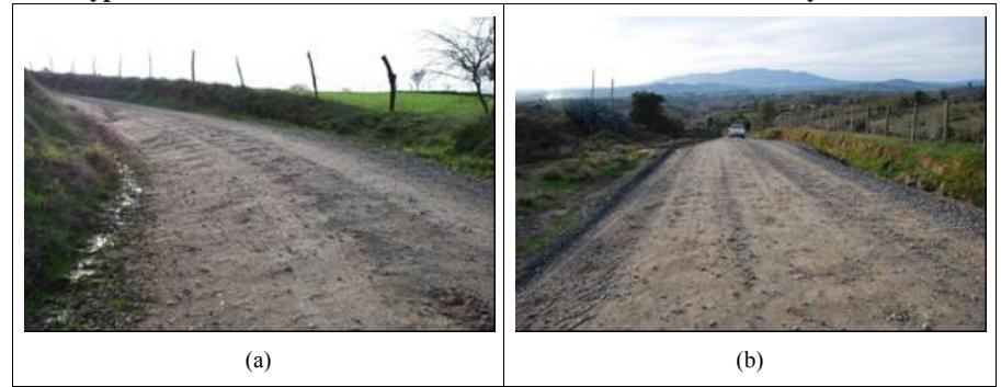
**Figure E.1.1 Corrugations in Roads (a) N462 and (b) N480**
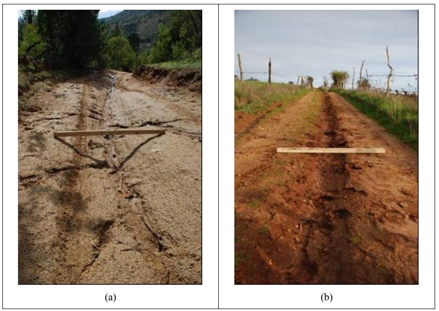
**Figure E.1.2 Erosion in Roads (a) N474 and (b) Local Road V\_BAB**

**Figure E.1.3 Drainage Problems in Roads (a) N498 and (b) Local Road V\_LLA**

**Figure E.1.4 Erosions Caused by Unstable River Banks and Drainage in Roads (a) N474 and (b) N620**
#### **E.2. Inventory Data Chile Case Study**
**Table E.2.1 Chile Case Study Inventory Data: Gravel Roads**
| | | | | | | Road Data | | | |
|-----------------|--------------|------------------|--------------------|-----------------|-----------------------------|------------------|-------------------------------------------------------------------------------------------------------------------------------------------------------------------------------|------------|----------------------------|
| Section
Code | Road
Code | Road
Category | Road
Length (m) | Surface
Type | Traffic
Volume
(AADT) | Traffic
Level | Traffic Characteristics | Population | Population
Proportion % |
| 2 | N620 | Secondary | 13900 | Gravel | 100 | Moderate | 3 buses*2, forestry trucks, trucks w ith
gravel from river, 1 ambulance*2, 2
school buses*2 | 210 | 3,8% |
| 3 | N496_R | Secondary | 2000 | Gravel | 30 | Low | Sum of traffic of tw o earth roads + 50%
additional traffic | 44 | 0,8% |
| 8 | N600 | Secondary | 9700 | Gravel | 70 | Moderate | 1bus*2, 2 school bus*2 | 560 | 10,0% |
| 14 | N490 | Secondary | 4000 | Gravel | 50 | Low | 2 commercial trucks
(vegetable/chicken)*2 | 80 | 1,4% |
| 15 | N480 | Secondary | 7700 | Gravel | 100 | Moderate | 2 buses*2, important traffic of forestry
trucks (3 forestry companies), important
traffic of agricultural truck + w orkers
bus, 2 school buses*2 | 648 | 11,6% |
| 16 | N462 | Secondary | 3300 | Gravel | 30 | Low | 1 ambulance*2, 1 school bus*2, muni,
comerciantes | 40 | 0,7% |
| 19 | N616 | Secondary | 3200 | Gravel | 20 | Low | 1 ambulance*2, commercial trucks | 36 | 0,6% |
| 20 | N486 | Secondary | 5800 | Gravel | 40 | Low | 1bus*2, 1 ambulance*2, 2 school bus *2 | 80 | 1,4% |
| 21 | N466 | Secondary | 11700 | Gravel | 80 | Moderate | 3 school bus*2, 3*bus*2, 5 forestry
trucks*2, 1 ambulance*2, important
traffic from municipality of Trehuaco | 320 | 5,7% |
| 26 | N482 | Secondary | 11200 | Gravel | 60 | Moderate | 2 school bus*2, 3*bus*2, 4 forestry
trucks*2, 1 ambulance*2 | 120 | 2,2% |
| 28 | N478 | Secondary | 5300 | Gravel | 80 | Moderate | 2 school bus*2, 3*bus*2, 8 forestry
trucks*2, 2 ambulance*2, important
traffic from municipality | 400 | 7,2% |
| 34 | N610 | Secondary | 10200 | Gravel | 60 | Moderate | 2bus*2, important traffic of forestry
trucks, some traffic of busses w ith
w orkers | 260 | 4,7% |
| 36 | N510 | Secondary | 4900 | Gravel | 40 | Low | 1 school bus*2 until entrance of the
road, traffic increases during summer | 100 | 1,8% |
| 37 | N60-R | Secondary | 15900 | Gravel | 220 | High | 3 school bus*2, 4*bus*2trips*2, 10 traffic
of forestry trucks, 2 ambulance*2,
important traffic from municipality | 1000 | 17,9% |
| 38 | N60-R | Secondary | 15900 | Gravel | 260 | High | 3 school bus*2, taxi, police,
7*bus*3trips*2, 10 traffic of forestry
trucks, 2 ambulance*2, important traffic
from municipality | 1000 | 17,9% |
| 39 | N68 | Secondary | 11000 | Gravel | 100 | Moderate | school bus*2, 2*bus*2, 2 ambulance*2,
important traffic from municipality (less
traffic since Confluencia Bridge is
restricted to heavy traffic, forestry
trucks) | 680 | 12,2% |
**Table E.2.2 Chile Case Study Inventory Data: Earth Roads**
| | Road Data
Traffic | | | | | | | | | | | | | |
|-----------------|----------------------|------------------|--------------------|-----------------|------------------|------------------|----------------------------------------------------------------------------------|------------|----------------------------|--|--|--|--|--|
| Section
Code | Road
Code | Road
Category | Road
Length (m) | Surface
Type | Volume
(AADT) | Traffic
Level | Traffic Characteristics | Population | Population
Proportion % | | | | | |
| 1 | V_LLA | Local | 550 | Earth | 4 | Low | Local traffic and municipal
pickup ocassionaly | 4 | 0,4% | | | | | |
| 4 | N496_T | Secondary | 2800 | Earth | 6 | Low | Local traffic and municipal
pickup ocassionaly | 28 | 3,0% | | | | | |
| 5 | V_QTA | Local | 1400 | Earth | 14 | Low | Local traffic and municipal
pickup ocassionaly | 30 | 3,2% | | | | | |
| 6 | V_CU1 | Local | 400 | Earth | 10 | Low | Local traffic and municipal
pickup ocassionaly | 21 | 2,3% | | | | | |
| 7 | V_CU2 | Local | 500 | Earth | 10 | Low | Local traffic and municipal
pickup ocassionaly | 30 | 3,2% | | | | | |
| 9 | N498 | Secondary | 2000 | Earth | 14 | Low | 1 school bus*2 | 75 | 8,0% | | | | | |
| 10 | V_BQH | Local | 850 | Earth | 8 | Low | 1 ambulance*2 | 10 | 1,1% | | | | | |
| 11 | N474 | Secondary | 5000 | Earth | 12 | Low | Local traffic and municipal
pickup ocassionaly | 20 | 2,1% | | | | | |
| 12 | V_BA1 | Local | 1500 | Earth | 30 | Low | 1 ambulance*2 | 40 | 4,3% | | | | | |
| 13 | V_BA2 | Local | 1800 | Earth | 8 | Low | Local traffic and municipal
pickup ocassionaly | 18 | 1,9% | | | | | |
| 17 | V_BAB | Local | 1100 | Earth | 6 | Low | Local traffic and municipal
pickup ocassionaly | 20 | 2,1% | | | | | |
| 18 | V_CAB | Local | 1700 | Earth | 6 | Low | NMT 2 horses carriages*2 | 16 | 1,7% | | | | | |
| 22 | N492 | Secondary | 6800 | Earth | 40 | Low | 1 school bus*2, 1*bus*2, 1
ambulance*2 | 105 | 11,3% | | | | | |
| 24 | V_HLB | Local | 1700 | Earth | 10 | Low | Local traffic and municipal
pickup ocassionaly | 10 | 1,1% | | | | | |
| 25 | V_LNJ | Local | 1200 | Earth | 16 | Low | Local traffic and municipal
pickup ocassionaly | 6 | 0,6% | | | | | |
| 27 | N500 | Secondary | 3000 | Earth | 20 | Low | 1 school bus*2, 1
ambulance*2 | 52 | 5,6% | | | | | |
| 29 | V_PSA | Local | 1300 | Earth | 16 | Low | 1 school bus*2, 1
ambulance*2, local traffic
1 ambulance 2, local traffic, | 20 | 2,1% | | | | | |
| 30 | V_CHU | Local | 3000 | Earth | 30 | Low | police and municipal pickup
ocassionaly | 120 | 12,9% | | | | | |
| 31 | V_AMI | Local | 2000 | Earth | 6 | Low | Local traffic and municipal
pickup ocassionaly | 20 | 2,1% | | | | | |
| 32 | N494 | Secondary | 5400 | Earth | 60 | Moderate | 1 ambulance*2, local traffic
and forestry trucks | 200 | 21,4% | | | | | |
| 33 | V_LPL | Local | 1600 | Earth | 30 | Low | 1 school bus*2, 1
ambulance*2, forest guard | 80 | 8,6% | | | | | |
| 35 | V_RCM | Local | 2000 | Earth | 10 | Low | Local traffic | 8 | 0,9% | | | | | |
#### **E3. Condition Evaluation Data Chile Case Study**
**Table E.3.1 Chile Case Study Condition Evaluation: Gravel Roads (Field 1 and 2)**
| Roa | d D
ata | | Pre | vio
Ma
inte
us
nan | and
Co
ndi
tion
Ev
alu
atio
ce
ns | Pre | vio
Ma
us | inte
nan
ce | and
Co
ndi
tion
Ev
alu
atio
ns |
|-------------|------------|------------------------------------------------------|----------|-------------------------------------------------------|-------------------------------------------------------------------------------------------------------------------------------------------------------------------------------------------------------------------------------|-----------------------------------------------------------------------------------------------------------------------------------------------------------------------------------------------------------------|-----------------|-------------------|------------------------------------------------------------------------------------------------------------------------------------------------------------------------------------------------------------------------------------------------------------------------------------------------------------------------------------------------------------------------------------------------------------------------------------------------------------------------------------------------|
| Sec
tion | Roa
d | | | | -08
sep | | | Ap | ril-0
9 |
| Cod
e | Cod
e | Pre
vio
us
Ma
inte
nan
ce | UPC
I | Co
ndi
tion | Co
ent
mm
s | Pre
vio
Ma
inte
us
nan
ce | UPC
I | Co
ndi
tion | Co
ent
mm
s |
| 2 | N62
0 | Gra
ding
Ma
y, Jun
e/08 | 7,1 | Goo
d | Dra
inag
rob
lem
(lac
k of
sid
e d
rain
nd s
lope
),
e p
s a
in w
hee
lpat
h ca
ion
ter
w a
use
s e
ros | Loc
al re
vel
and
ding
gra
gra
/08
, Se
pril/
(el
Aug
pt 0
8, A
09
ce)
. Gr
adin
g S
, Oc
t, N
ept
sau
ov, | 8,1 | y G
Ver
ood | Ove
rsiz
ed g
ular
teria
l in
Km
6.3
incr
ugh
s in
ran
ma
ese
s ro
nes
slop
e |
| 3 | N49
6_R | Brid
d Jun
lace
ge
rep
e/08 | 3,5 | Ver
y P
oor
(w i
e)
nter
clo
sur | Sec
tion
inte
r clo
e d
ud,
t of
ts w
ue t
pre
sen
sur
o m
res
d in
bet
ter
ditio
roa
con
n | Loc
al re
vel
and
ding
Au
gra
gra
g,
Sep
t/08
/09
. Lo
cal
ding
Jan
gra | 8,4 | Ver
y G
ood | Lac
k of
nula
teria
l, av
aila
ble
vel
ts
gra
r ma
gra
pre
sen
rsiz
e. P
dra
inag
hee
lpat
hs.
Km
0.3
and
Km
1.4
ove
oor
e o
n w
ts im
tant
sion
, riv
rote
ctio
hou
ld b
pre
sen
por
ero
er p
ns s
e
rein
forc
ed.
Km
w it
h ro
ugh
rob
lem
s d
0.6
ue t
nes
s p
o
f a
k.
pre
sen
ce o
roc |
| 8 | N60
0 | | 6,8 | Goo
d | Irre
gula
rofi
le, r
uttin
d by
lac
k
r tra
nsv
ers
e p
g ca
use
of g
el. E
ion
obs
ed
in fi
rst
kilom
ete
r of
the
rav
ros
erv
d.
roa | Reg
el a
nd g
rad
ing
Sep
t/08
rav
rch/
Loc
al g
rad
ing
Jan
, Ma
09 | 9 | Ver
y G
ood | Lac
k of
nula
teria
l in
l se
ctio
f th
ad
gra
r ma
sev
era
ns o
e ro
atio
Rutt
ing
sed
by
late
d
cau
ses
co
rrug
ns.
cau
acc
umu
eria
l in
the
of t
he r
oad
. Gr
adin
d.
mat
tre
este
cen
g s
ugg |
| 14 | N49
0 | | 6,3 | Goo
d | Ero
sion
in s
ions
w it
h st
slo
ect
eep
pes | Gra
ding
No
v, D
ic/0
8 , J
Feb
an,
,
Mar
ch/0
9 (lo
cal) | 7,4 | Goo
d | Irre
gula
r tra
rofi
le c
rutt
ing
in h
oriz
onta
l
nsv
ers
e p
aus
es
cur
ves |
| 15 | N48
0 | Gra
ding
Jun
e/08 | 6,5 | Goo
d | Cor
atio
ns i
n st
slo
rug
eep
pes | Gra
ding
Oc
t, N
ov/0
8 | 4,8 | Reg
ular | Roa
d w
ith g
ood
file,
but
ts im
atio
tant
pro
pre
sen
por
co
rrug
ns
in s
ect
ions
w it
h sl
ope
s |
| 16 | N46
2 | | 3,9 | Poo
r | Ero
sion
d co
atio
ns i
n st
slo
an
rrug
eep
pe | | 2,4 | Ver
y P
oor | Cor
atio
ns i
n sl
s. L
l ero
sion
blem
du
e to
rug
ope
oca
pro
po
or
side
dra
inag
e. |
| 19 | N61
6 | Reg
el &
rav
gra
ding
Se
pt/0
8 | 8,3 | Ver
y G
ood | Gra
d. S
urfa
ding
d tr
lope
uire
an
ans
ver
se s
req
ce
w it
h go
od
eria
l.
mat | Gra
ding
Jan
/09 | 8,3 | Ver
y G
ood | d. G
Rutt
ing,
ding
uire
ood
vel
late
d in
the
gra
req
gra
acc
umu
side
s of
the
d.
roa |
| 20 | N48
6 | | 4,7 | Reg
ular | Lac
k of
teria
l an
d s
ide
slop
e. O
size
d
ma
ver
ate
duc
gh s
urfa
agg
reg
pro
es
rou
ce. | Gra
ding
Oc
t, N
ov/0
8; C
ulve
rt
t Oc
t/08
lace
rep
men | 5,5 | Goo
d | Cor
atio
lack
of
vel
to im
irre
gula
r tra
rug
ns,
gra
pro
ve
nsv
ers
e
file.
Ove
rsiz
ed a
tes
incr
ugh
s of
the
pro
ggr
ega
eas
e ro
nes
d.
roa |
| 21 | N46
6 | Gra
ding
Ma
y, Jun
e, S
ept/
08 | 9,4 | Ver
y G
ood | Gra
ding
uire
d, c
gat
ions
ob
ved
in s
tee
req
orru
ser
p
slop
es. | Gra
ding
Oc
t, N
ov/0
8 | 6,3 | Goo
d | Roa
d in
ral g
ood
ndit
ion,
ecif
ic s
ect
ions
t
a g
ene
co
sp
pre
sen
slig
ht c
ions
d ru
tting
. Gr
adin
quir
ed,
d
gat
orru
an
g re
goo
mat
eria
l av
aila
ble
in th
ides
of
the
d.
e s
roa |
| 26 | N48
2 | Brid
olap
sed
ge c
Aug
/08 | 7,2 | Goo
d | Lac
k of
nula
teria
l, se
ctio
ith e
ion
gra
r ma
ns w
ros
affi
and
ized
gate
s. Im
tant
bu
s tr
ov
ers
ag
gre
por
c. | Loc
al g
rad
ing
Feb
, Ma
rch/
09.
Loc
al re
vel
Mar
ch/0
9 (u
f
gra
se o
rsiz
e riv
te)
ove
er a
ggr
ega | 8 | Ver
y G
ood | Roa
d p
ized
nula
teria
l. Dr
aina
ents
res
ov
ers
gra
r ma
ge
blem
d by
vel
late
in t
he s
ides
of
the
pro
s ca
use
gra
acc
umu
d.
roa |
| 28 | N47
8 | Gra
ding
Ma
y, Sep
t/08 | N,E | | Not
alua
ted
, bla
der
rkin
ev
w o
g | Gra
ding
d re
vel
9/A
pril/
09
an
gra | 8 | Ver
y G
ood | Poth
oles
in s
ions
w it
h po
ion
of g
ular
ect
act
or c
omp
ran
mat
eria
l, ob
ved
atio
ith e
xte
nde
d
ser
as
cor
rug
ns w
vele
ngth
w a
s |
| 34 | N61
0 | Gra
ding
May
e, S
ept/
,Jun
08 | 10 | Ver
y G
ood | Roa
d in
od c
ond
ition
tion
ith l
l
go
, so
me
sec
s w
oca
sion
blem
ero
pro
s. | Reg
el N
ov/0
8; G
rad
ing
Oct
rav
,
Nov
/08
. Lo
cal
(Me
mbr
illar
)
ding
in e
rod
ed s
ion
ect
gra
Mar
ch/0
9 | 7,7 | Goo
d | Slig
ht c
gat
ion
in s
lope
s. G
ood
file
and
nula
orru
pro
gra
r
obs
ed
in th
ad
erv
e ro |
| 36 | N51
0 | Loc
vel Aug
al re
gra
/08 | 5,9 | Goo
d | Ove
rsiz
ular
teria
l in
all t
he s
ect
ion,
e g
ran
ma
po
or
ghn
, loc
al d
rain
blem
s d
urin
inte
rou
ess
age
pro
g w
r. | ch/0
Loc
al g
rad
ing
Mar
9
(Rin
ávid
a)
com | 5,4 | Reg
ular | l. Si
Poth
oles
aire
d w
ith g
ular
teria
de d
rain
ed t
rep
ran
ma
s ne
o
be c
lear
ed.
Imp
uttin
g ob
ved
in s
ctio
ortn
at r
ser
ome
se
ns. |
| 37 | N60
-R | | N,E | | | Gra
ding
Se
pt, O
Nov
/08
. Lo
cal
ct,
/09
(Po
ding
Jan
rtez
uelo
gra
Pan
guil
). L
l reg
el
emu
oca
rav
Feb
/09
(Or
illa) | 10 | Ver
y G
ood | Gra
ding
uire
d, g
ood
vel
late
d in
the
sid
f
req
gra
acc
umu
es o
the
d
roa |
| 38 | N60
-R | | N,E | | | Gra
ding
Se
pt, O
ct,
Nov
/08
. Lo
cal
ding
Jan
/09
(Po
uelo
rtez
gra
Pan
guil
).
emu | 8,26 | Ver
y G
ood | file,
Irre
gula
r lon
gitu
dina
l pro
sim
ilar
to c
gat
ions
d
orru
, ca
use
by p
ctio
n of
nula
teria
l
oor
co
mpa
gra
r ma |
| 39 | N68 | | N,E | | | Gra
ding
Se
pt, O
ct/0
8.
Loc
al
eb/0
9 (O
)
el F
rilla
reg
rav | 10 | Ver
y G
ood | Gra
ding
uire
d, g
ood
vel
late
d in
the
sid
f
req
gra
acc
umu
es o
the
d
roa |
**Table E.3.2 Chile Case Study Condition Evaluation: Gravel Roads (Field 3 and 4)**
| Sec
tion | Roa
d | | | -09
sep | | sep | -10 | | oct | -11 | | |
|-------------|------------|--------------------------------------------------------------------------------------------------------------------------------------------------------------------------------------------------------------------------------------------------------------------------------------------------------|----------|-------------------|-----------------------------------------------------------------------------------------------------------------------------------------------------------------------------------------------------------------------------------------------------------------------------------------------------------------------------------------------------------------------------------------------|----------------------------------------------------------------|----------------------------------|----------------------------------------------------------------------------------------------------------------------------------------------------------------------------------------------------|---------------------------------------------------------------------|----------------------------------|----------|-------------------|
| Cod
e | Cod
e | Pre
vio
Mai
nte
us
nan
ce | UPC
I | Con
diti
on | Com
nts
me | 0 M
aint
201
typ
e | 0 M
aint
201
Effe
ct | 201
1 M
aint
ena
nce | 201
1 M
aint
typ
e | 1 M
aint
201
Effe
ct | UPC
I | Con
diti
on |
| 2 | N62
0 | Loc
al re
el a
nd g
radi
ng (
Sau
ce)
Apr
il,
grav
e/09
Jun | 6,2 | Goo
d | Poo
r dr
aina
rodu
sion
tha
tra
t
ge p
ces
nsv
erse
ero
the
d, c
ulve
rt ha
be
nde
d.
s to
exte
cros
ses
roa
Beg
innin
g of
tion
ts p
otho
les
of m
ode
rate
sec
pre
sen
erity
sev | Prev
enti
ve
Gra
ding | 3,5 | Perf
ilado
z al
un
a ve
mes
(sec
ción
eba
), rip
io
pru
prim
1,5
kms
. Se
eros
real
izó
nch
e lo
cal
un e
nsa
(glo
bal) | Prev
enti
ve
Gra
ding
Reh
abili
tatio
n | 4,25 | 8,3 | Ver
y G
ood |
| 3 | N49
6_R | Loc
al g
radi
nd r
vel
Aug
/08.
Loc
al
ng a
egra
grad
ing
and
l em
reg
rave
erge
ncy
are
a
Jun
e, J
uly/
09.
Gra
ding
ek b
efor
w e
e
luat
ion
(28/
Sep
t/09
)
eva | 2,8 | Poo
r | One
sid
e of
the
d pr
late
d gr
l,
nts
roa
ese
acc
umu
ave
erat
ing
drai
oble
and
ter a
mula
tion
gen
nag
e pr
ms
w a
ccu
in th
hee
l pat
h. R
oad
face
ts p
natu
ral
e w
sur
pre
sen
oor
eria
l.
mat | Mini
mum
Gra
ding | 1 | 1 Pe
rfila
do a
l rea
lizad
nua
o
icipa
lidad
por
mun | Mini
Gra
ding
mum | 1 | 6,1 | Goo
d |
| 8 | N60
0 | Brid
ired
(Cu
cha
Urr
ejola
) ap
ril/0
9,
ge r
epa
Rloc
al re
el (C
uch
d Ll
ahu
en)
May
grav
a an
,
/09.
July
Loc
al re
el in
grav
em
erge
ncy
tion
(Cu
cha
Urr
ejola
) Au
g/09
sec | 5,7 | Goo
d | Effe
ctiv
ad w
idth
is r
edu
ced
by
ion
in s
ide
etat
e ro
veg
drai
Rutt
ing
ting
ar d
ide
star
to a
ue t
ns.
ppe
o po
or s
e. C
slop
gati
sta
rting
to a
ar in
w h
eelp
aths
orru
ons
ppe
w ith
lac
k of
vel.
gra | Loc
al R
vel
egra
+ M
inim
um
Gra
ding | 2,5 | 3 Pe
rfila
dos
ales
anu
vial
idad
tiró
ripi
, se
o en
tore
che
sec
s co
n en
san
de v
ialid
ad | Loc
al R
vel
egra
+
Gra
Mini
ding
mum | 2,5 | 9,5 | Ver
y G
ood |
| 14 | N49
0 | Loc
al g
radi
nd r
vel
(Ca
rrull
a)
ng a
egra
anc
Apr
il, M
Jun
e, A
ug/0
9 an
d M
ay,
ayo
,
io/0
9 (B
s).
Jun
s A | 6,2 | Goo
d | Slig
ht c
gati
in i
nter
nal w
hee
lpat
h in
hori
tal
orru
ons
zon
e. In
the
fut
dai
oble
ould
curv
ure,
nag
e pr
m c
cau
se
f the
ion
in th
e si
de o
d.
eros
roa | Prev
enti
ve
Gra
ding | 3,5 | 2 Pe
rfila
dos
ales
anu
real
izad
os p
or
icipa
lidad
mun | Prev
enti
ve
Gra
ding | 3,5 | 7,7 | Goo
d |
| 15 | N48
0 | Gra
l 5/J
uly/
09)
ding
and
reg
rave | 6,5 | Goo
d | Goo
d si
de d
rain
s. R
oad
uire
lling
of
req
s gr
ave
new
mat
eria
l an
d gr
adin
ater
ial a
mula
ted
in th
e si
de.
g m
ccu
Com
tion
uire
d in
tion
ith c
gati
pac
req
sec
s w
orru
ons | Mini
mum
Gra
ding | 1 | 2 Pe
rfila
dos
ales
anu
vial
idad | Gra
Mini
ding
mum | 1 | 7,1 | Goo
d |
| 16 | N46
2 | Gra
ding
Ma
y/09 | 4,2 | Poo
r | Side
sion
and
tion
in s
lope
ood
dra
inag
ero
cor
ruga
s, g
e
and
file
thou
gh.
Mat
eria
l req
uire
d in
slo
pro
pes | Prev
enti
ve Gra
ding | 3,5 | 2 Pe
rfila
dos
ales
anu | Prev
enti
ve Gra
ding | 3,5 | 3,4 | Poo
r |
| 19 | N61
6 | | 9 | Ver
y G
ood | Rutt
ing
sed
by
r sid
e sl
. Go
od g
l, ro
ad
cau
poo
ope
rave
in g
ral is
in v
d co
ndit
ion
ene
ery
goo | Mini
mum
Gra
ding | 1 | No
antu
n 20
11
se m
vo e | No
main
tena
nce | 0 | 8,3 | Ver
y G
ood |
| 20 | N48
6 | Loc
al re
el M
ay/0
9 an
d gr
adin
g Ju
grav
ne,
July
/09
(Ca
brer
ía) | 7,6 | Goo
d | Gra
vel
ired
atio
nd p
side
slo
requ
, co
rrug
ns a
oor
pes | Prev
enti
ve Gra
ding | 3,5 | 2 Pe
rfila
dos
ales
anu
vial
idad | Prev
enti
ve Gra
ding | 3,5 | 7,7 | Goo
d |
| 21 | N46
6 | Brid
nd e
rosi
ired
in
ge a
on r
epa
Pan
guile
culv
epla
ced
in C
abre
ría
ert r
mu+
Jun
e/09
. Re
el in
rive
ing
in
grav
r cr
oss
g, S
ept/
Pan
guile
July
, Au
09
mu | 5,5 | Goo
d | Cor
tion
s ob
ed i
n ho
rizo
ntal
e.Si
de s
lope
ruga
serv
curv
s
d to
be
impr
d an
d si
de d
rain
ed t
o be
nee
ove
s ne
clea
ned
. Ro
ad p
nts
d co
ndit
ion
in g
ral.
rese
goo
ene | Mini
mum
Gra
ding | 1 | 4 pe
rfila
dos
ales
anu
(Glo
bal) | Gra
Mini
ding
mum | 1 | 9,5 | y G
Ver
ood |
| 26 | N48
2 | Eros
ion
ired
hoo
l Jun
e/09
repa
nea
r sc
,
oyá
n Se
pt/0
brid
ired
in T
9
ge r
epa
ranc | 6,5 | Goo
d | Wid
d go
od s
ide
drai
Dra
inag
oble
sed
e an
ns.
e pr
ms
cau
by p
side
slo
thol
tart
ing t
oor
pes
, po
es a
re s
o ap
pea
r. | Prev
enti
ve Gra
ding | 3,5 | PIR
Car
el s
ecto
r
Tra
. Tra
ba
nco
yan
mo
prue
ripio
rfiló
Clar
y pe
o y | Reh
abili
tatio
n | 5 | 8,4 | Ver
y G
ood |
| 28 | N47
8 | Gra
ding
Se
pt/0
9 | 5,8 | Goo
d | Gra
vel
ired
. Sid
e sl
ds t
o be
imp
d.
requ
ope
nee
rove
Cor
tion
d po
thol
ing t
tart
ruga
s an
es a
re s
o ap
pea
r.
Con
ditio
befo
re 1
8/Se
ulat
ion
pt, w
ater
n w
as p
oor
cum
in o
hee
lpat
h w
olve
d w
ith g
radi
ne w
as s
ng. | Mini
mum
Gra
ding | 1 | 2 Pe
rfila
dos
ales
anu
por
icipa
lidad
mun | Mini
Gra
ding
mum | 1 | 7,0 | Goo
d |
| 34 | N61
0 | Gra
ding
Ap
ril, S
ept/
09 a
nd l
l reg
l
oca
rave
Jun
e, J
uly/
09 | 6,5 | Goo
d | Sec
tion
w it
h go
od g
l, pr
ofile
and
dra
inag
e. M
ain
rave
prob
lem
sed
by
mod
atio
w h
ich t
erat
cau
e co
rrug
ns,
urn
to b
in s
teep
slo
e se
vere
pes | Mini
mum
Gra
ding | 1 | 4 pe
rfila
ño (Glo
dos
al a
bal) | Gra
Mini
ding
mum | 1 | 5,0 | Reg
ular |
| 36 | N51
0 | Loc
al g
radi
ng R
inco
máv
ida A
ug/0
9 | 6,5 | Goo
d | Dra
inag
e in
ular
ditio
ide
slop
quir
ed.
reg
con
n, s
e re
Rutt
ing
obs
d, g
radi
ired
. Ero
sion
is n
ot
erve
ng r
equ
tran
sve
rse. | Mini
mum
Gra
ding | 1 | 2 Pe
rfila
do a
l rea
lizad
nua
o
icipa
lidad
por
mun | Mini
Gra
ding
mum | 1 | 9,2 | Ver
y G
ood |
| 37 | N60
-R | Loc
al g
radi
ng P
orte
lo-C
hud
al M
zue
ay,
Aug
, 10
/sep
t/09 | 5,5 | Goo
d | Gra
vel
ired
thol
nd c
gati
for
med
by
requ
, po
es a
orru
ons
brak
ing
e in
the
e of
brid
entr
zon
anc
ge. | Mini
mum
Gra
ding | 1 | 3 Pe
rfila
do a
l rea
lizad
nua
o
vial
idad
por | Les
s th
an Mini
Gra
ding
mum | 1 | 6,2 | Goo
d |
| 38 | N60
-R | | N.E | N.E | | Mini
mum
Gra
ding | 1 | 3 P
erfil
ado
al
anu
real
izad
r via
lidad
o po | Les
s th
an Mini
Gra
ding
mum | 1 | 5,9 | Goo
d |
| 39 | N68 | Ori
ay/0
Loc
al re
el in
lla M
9, E
grav
mer
gen
cy
l an
d gr
adin
g of
sion
in O
rilla
regr
ave
ero
Jun
e/09 | 8,8 | Ver
y G
ood | Wat
mula
ted
in th
e si
de o
f the
d ca
d by
er a
ccu
roa
use
r sid
e sl
ulve
rt. In
the
end
of t
he s
ecti
to c
poo
ope
on
(ho
e), g
sligh
t rut
ting
rizo
ntal
l req
uire
d to
curv
rave
solv
e th
oble
e pr
m | Mini
mum
Gra
ding | 1 | 3 Pe
rfila
do a
l rea
lizad
nua
o
vial
idad
por | Mini
Gra
ding
mum | 1 | 6,3 | Goo
d |
**Table E.3.3 Chile Case Study Condition Evaluation: Earth Roads (Field 1 and 2)**
| | | | | sep | -08 | | | Apr
il-09 | |
|-------------------------|----------------------|---------------------------------------------|----------|-------------------------------------------------|------------------------------------------------------------------------------------------------------------------------------------------------------------------------------------------------------------------------------------------------------------------------------------------------------------------|-----------------------------------------------------------------------------------------------------------------------------|----------|-------------------|-----------------------------------------------------------------------------------------------------------------------------------------------------------------------------------------------------------------------------------------------------------------------------------------------------------|
| Sec
tion
Cod
e | Roa
d
Cod
e | Pre
viou
s
Mai
nte
nan
ce | UPC
I | Con
diti
on | Com
nts
me | Pre
viou
s M
aint
ena
nce | UPC
I | Con
diti
on | Com
nts
me |
| 1 | V_L
LA | | 5,8 | Ver
y Po
or (w in
losu
re)
ter c | Ver
ond
ition
, w i
nter
clo
sed
by
y po
or c
sure
cau
poo
r
drai
d m
ud.
nag
e an | | 7,4 | Goo
d | |
| 4 | N49
6_T | | 3,1 | Ver
y Po
or (w in
ter c
losu
re) | Ver
ond
ition
, w i
nter
clo
sed
by
y po
or c
sure
cau
poo
r
drai
d m
ud.
nag
e an | Loc
al g
radi
ng J
an/0
9 | 5,4 | Reg
ular | Loc
al d
rain
blem
in K
m 0
.6, c
ulve
issin
rt m
age
pro
g.
Ove
rsiz
ed g
l in s
urfa
Nar
d w
ith p
rave
ce.
row
roa
oor
grad
ing.
Poth
oles
sta
rting
to a
ar in
slo
ppe
pes |
| 5 | V_Q
TA | | 4,6 | Ver
y Po
or (w in
losu
re)
ter c | Impo
rtan
t ero
sion
blem
s at
the
end
of t
he r
oad
pro
w in
losu
ter c
cau
ses
re. | Loc
al g
radi
ng J
an/0
9 | 6 | Goo
d | Eros
ion
in s
lope
s, d
rain
and
tran
prof
ile n
eed
age
sve
rse
s
to b
e in
ed i
ctio
ith p
robl
prov
n se
ns w
ems |
| 6 | V_C
U1 | | 7,7 | Ver
y G
ood | Loc
al d
rain
blem
age
pro
s | Loc
al g
radi
ng J
Mar
ch/0
9
an, | 4,3 | Reg
ular | |
| 7 | V_C
U2 | | 4,9 | Reg
ular | Drai
oble
in so
ecti
d ac
ulate
d
nag
e pr
ms
me s
ons
, mu
umm
betw
w h
eelp
aths
. Ve
oad
een
ry n
arro
w r | Loc
al g
radi
ng J
Mar
ch/0
9
an, | 7,8 | Goo
d | |
| 9 | N49
8 | | 2,8 | Ver
y Po
or (w in
losu
re)
ter c | Exc
esiv
osio
n in
the
w he
el p
ath
prod
ad
e er
uce
s ro
clos
Som
ctio
nt d
osio
n in
ure.
e se
ns p
rese
ang
erou
s er
the
side
of t
he r
oad
. Gr
l obs
d in
ctio
ave
erve
som
e se
ns. | Gra
ding
Sep
t/08 | 9,2 | Ver
y G
ood | Exc
of g
l acc
lated
in t
he s
ide o
f the
d,
ess
rave
umu
roa
ds g
radi
nd c
ctio
ith d
rain
ing s
yste
m. S
nee
ng a
one
ns w
ome
ion c
ed b
y riv
eed
to b
info
rced
eros
aus
er n
e re |
| 10 | V_B
QH | | 4,7 | Reg
ular | Poth
oles
in w
hee
lpat
hs a
nd r
uttin
d by
g ca
use
poo
r
drai
e. A
f an
bula
uire
d.
nag
cce
ss o
am
nce
req | Gra
ding
Au
g/08 | 5,6 | Goo
d | |
| 11 | N47
4 | | 2,3 | Ver
y Po
or (per
losu
re)
m. c | Extr
sion
of w
hee
lpat
hs o
bse
rved
in s
lope
eme
ero
s.
Sec
tion
in K
m 2
.1 p
nts
dan
rosi
on i
n th
rese
gero
us e
e
side
of t
he r
oad | Gra
ding
and
l Se
pt/0
8
reg
rave
(Sec
is),
Gra
tor L
os M
ding
aqu
Dic/
08 | 6,4 | Goo
d | Rec
grad
ing i
d er
osio
oble
bse
rved
afte
ent
mpr
ove
n pr
m o
r
w in
ter.
Reg
ular
rutt
ing o
bse
rved
w it
hin a
nd b
etw
een
w he
el p
aths |
| 12 | V_B
A1 | | 3,7 | Ver
y Po
or (w in
ter c
losu
re) | Impo
sion
and
ter f
low
in ce
line
sed
rtan
t ero
ntre
w a
cau
by p
drai
oor
nag
e. | Gra
ding
Dic
/08
and
Jan
/09 | 3,6 | Poo
r | |
| 13 | V_B
A2 | | 3,7 | Ver
y Po
or (w in
losu
re)
ter c | Impo
sion
and
ter f
low
in ce
line
sed
rtan
t ero
ntre
w a
cau
by p
drai
oor
nag
e. | Gra
ding
Dic
/08
and
Jan
/09 | N.
E | | |
| 17 | V_B
AB | | 7 | Goo
d | Eros
ion o
bse
rved
in c
entr
eline | | 6,6 | Goo
d | |
| 18 | V_C
AB | | 3,3 | Poo
r | Impo
rtan
t ero
sion
sed
by
r dra
inag
e. W
inte
cau
poo
r
clos
. Cu
lver
t mis
sing
in a
tion
ures
sec | Culv
ir Oc
t/08
ert r
ding
epa
, gra
Ene/
09 | 7,3 | Goo
d | Side
Eros
ion
in ce
ntre
line
sed
by
hou
tran
sit.
dra
in
cau
rse
ired
in s
ide o
f the
d
requ
roa |
| 22 | N49
2 | | 6,2 | Goo
d | Lac
k of
sel
d m
ial, e
sed
ks a
bse
rved
ecte
ater
xpo
roc
re o | Gra
ding
Nov
/08 | 8,4 | Ver
y G
ood | Clay
soi
l, ov
ersi
zed
mula
ted
in th
ad
te a
agg
rega
ccu
e ro
side
l req
uire
d.
s, g
rave |
| 24 | V_H
LB | Gra
ding
Sep
t/08 | 5 | Reg
ular | Impo
rtan
t ero
sion
blem
s, h
inte
pro
ow e
ver
no w
r
clos
of r
oad
obs
d. S
tion
nt
ures
are
erve
ome
sec
s pr
ese
rsiz
ed g
l.
ove
rave | Gra
ding
Nov
/08 | 3,1 | Poo
r | |
| 25 | V_L
NJ | | 5,4 | Reg
ular | Som
osio
oble
inte
r clo
s of
d ar
e er
n pr
ms,
no w
sure
roa
e
obs
d.
erve | | 7,1 | Goo
d | |
| 27 | N50
0 | | 3,4 | Poo
r | Impo
rtan
t ero
sion
and
file
defo
tion
s in
both
pro
rma
w he
elpa
ths
sed
by
r dra
inag
e. C
ulve
rt m
issin
g in
cau
poo
km 2
.2 | Loc
al g
radi
ng F
eb,
Mar
ch/0
9 | 6,7 | Goo
d | Rou
gh s
urfa
ed b
bed
ded
rsiz
l,
ce c
aus
y em
ove
e gr
ave
rutti
es i
ular
tran
prof
ile.
ng c
aus
rreg
sve
rse |
| 29 | V_P
SA | | 4,9 | Reg
ular | | | 5,4 | Reg
ular | |
| 30 | V_C
HU | | 6,2 | Goo
d | Poo
r tra
file
sion
od s
ide
nsv
erse
pro
cau
ses
ero
, go
drai
ns. | | 5,3 | Reg
ular | Rou
gh s
urfa
ed b
bed
ded
rsiz
l,
ce c
aus
y em
ove
e gr
ave
rutti
f 7c
m in
w h
eelp
ath,
sid
e dr
ain
ired
ng o
one
requ |
| 31 | V_A
MI | | 5,4 | Reg
ular | Sec
tion
nt s
urfa
ce d
efor
mat
ions
and
sion
s pr
ese
ero
sed
by
r dra
inag
cau
poo
e.
Inter
l roa
bus
ice b
etw | | 6,5 | Goo
d | Ove
rsiz
ed g
l, irr
lar t
ofile
rave
egu
rans
vers
e pr
Impr
t of
prof
ile a
nd c
lean
ing o
f dr
aina
ired
ove
men
ge r
equ |
| 32 | N49
4 | | 8,2 | Ver
y G
ood | icipa
d, p
nts
mun
rese
serv
een
Chu
dal
and
N60
. Po
thol
tion
ized
es,
corr
uga
s, o
vers
nd la
ck o
f gr
l in s
ectio
ith b
te a
agg
rega
ave
n w
us
ice
serv | | 6,7 | Goo
d | Gra
vel
ired
. Tra
ffic
of f
try T
ruck
irre
gula
requ
ores
s ca
use
r
prof
of g
ile. L
ack
l ca
atio
nd p
otho
les.
rave
use
s co
rrug
ns a |
| 33 | V_L
PL | | 5,8 | Goo
d | Poo
r sid
e sl
and
dra
ins.
Thin
silt
surf
duc
ope
ace
pro
es
dus
t pro
blem
s. | Gra
Oc
t/08
ding | 5,5 | Goo
d | |
| 35 | V_R
CM | | 3,2 | Poo
r | Surf
def
atio
rosi
nd w
inte
r clo
ace
orm
n, e
on a
sure
s
sed
by
r dra
inag
cau
poo
e. | Gra
ding
Ma
rch/
09 | 4,8 | Reg
ular | |
**Table E.3.4 Chile Case Study Condition Evaluation: Earth Roads (Field 3 and 4)**
| Roa | d Da
ta | | Pre
viou | s M
aint
ena
nce | and
Co
ndit
ion
Eva
luat
ions | | | Pre
viou
s M
aint
ena
nce | and
Co
ndit
ion | Eva
luat
ions | | |
|-------------|------------|---------------------------------------------------------------------------------------------------------------------------------------------------------------------------|-------------|---------------------------|-----------------------------------------------------------------------------------------------------------------------------------------------------------------------------------------------------------------------------------------------------------------------------------------------------------------------------------------------------------------------------------------------|-----------------------------------|--------------------|-----------------------------------------------------------------------------------------------------------------|---------------------------------------------------------|---------------------|----------|-------------------|
| | | | | | -09
sep | sep | -10 | | oct- | 11 | | |
| Sec
tion | Roa
d | | | | | 201
0 M
aint | 201
0 M
aint | | | 201
1 M
aint | | |
| Cod
e | Cod
e | Pre
viou
s M
aint
ena
nce | UPC
I | Con
ditio
n | Com
nts
me | type | Effe
ct | 201
1 M
aint
ena
nce | 201
1 M
aint
typ
e | Effe
ct | UPC
I | Con
ditio
n |
| 1 | V_L
LA | Grad
ing a
nd r
vel i
ction
egra
n se
w ith
inte
r clo
eme
rgen
cy w
sure
y/09
tion
June
, Jul
ding
sec
; gra | 7,7 | y Go
Ver
od | Side
dra
ins o
nly o
e sid
e of
the
d an
d us
than
half
w id
th
n on
roa
es m
ore
of c
arria
Sligh
sion
of o
hee
lpath
used
by
t ero
w at
gew
ay.
ne w
cas
er
flow
file.
f roa
or tr
First
300
d pr
nt im
port
ant
, po
ansv
erse
pro
m o
ese | Mini
mum
Gra
ding | 1 | 1 Pe
rfilad
ual r
ealiz
ado
o an
icipa
lidad
por
mun | Gra
Mini
ding
mum | 1 | 4,9 | Reg
ular |
| 4 | N49
6_T | Aug
/09
(ma
in ro
ad?
)
Gra
ding
July
/09
and
ious
prev
k 28
/Sep
t/09
)
w ee | 6,3 | Goo
d | poth
oles
(+ 1
m lo
ng),
vel r
ired
to re
pair
gra
equ
Ove
rsize
d gr
l pla
ced
in sl
s 3 y
. Sid
e dr
ains
only
at o
ave
ope
ears
ago
ne
side
. Pro
blem
ith s
relev
ation
in c
, sho
uld b
ted
s w
upe
urve
e co
rrec | Mini
mum
Gra
ding | 1 | 1 Pe
rfilad
ado por
ual r
ealiz
o an
icipa
lidad
mun | Mini
Gra
ding
mum | 1 | 7,1 | Goo
d |
| 5 | V_Q
TA | No m
ainte
nanc
e | 2 | Poo
r | Sec
tion
not e
valu
ated
it w a
s im
able
bec
e of
ion
as
pass
aus
sev
ere
eros | Mini
mum
Gra
ding | 1 | 1 Pe
rfilad
ado por
ual r
ealiz
o an
icipa
lidad
mun | Mini
Gra
ding
mum | 1 | 2,1 | Ver
y Po
or |
| 6 | V_C
U1 | Loc
al re
el ju
ly/09
grav | 6,8 | Goo
d | Goo
d su
rfac
nditi
on b
of g
l fro
m th
e riv
lace
d in
e co
eca
use
rave
er p
slop
es. T
osio
used
by
er fl
ide d
rains
w at
to s
rans
vers
e er
n ca
ow | Mini
mum
Gra
ding | 1 | 1 Pe
rfilad
ado por
ual r
ealiz
o an
icipa
lidad
mun | Mini
Gra
ding
mum | 1 | 7,6 | Goo
d |
| 7 | V_C
U2 | Loc
al re
eling
july
/09
grav | 6,5 | Goo
d | Ove
rsize
d ag
id fo
ion o
f mu
d an
d po
thole
s. Im
ates
rmat
port
ant
greg
avo
poth
oles
obs
d in
sect
ions
w it
hout
rsize
d ag
ates
erve
ove
greg | Mini
mum
Gra
ding | 1 | Sin
ión
tenc
man | No m
ainte
nanc
e | 0 | 6,7 | Goo
d |
| 9 | N49
8 | | 7,3 | Goo
d | Fou
r imp
orta
nt po
thole
ith w
ater
and
e de
form
ation
of
s w
som
w he
elpa
ths. | Mini
mum
Gra
ding | 1 | 2 Pe
rfilad
les v
ialida
d
os a
nua | Prev
entiv
e Gra
ding | 3,5 | 7,7 | Goo
d |
| 10 | V_B
QH | Grad
ing 1
6/se
pt/09
. Gra
vel a
nd
culv
lace
d in
tion
w ith
ert p
sec
drai
and
sion
blem
nage
ero
pro | 4 | Reg
ular | Poth
oles
(ma
x 1.
long
), irr
lar p
rofile
sion
in th
hee
l pat
h.
5 m
egu
, ero
e w
No p
abilit
oble
ms d
uring
rain
ass
y pr | Mini
mum
Gra
ding | 1 | 1 Pe
rfilad
ual r
ealiz
ado
o an
in man
icipa
lidad
por
mun
o s
tenc
ion | Mini
Gra
ding
mum | 1 | 4,4 | Reg
ular |
| 11 | N47
4 | Loca
l reg
l sec
tor l
is
rave
os m
aqu
june
/09,
ding
/09
(ma
in
gra
aug
road
?) | 4 | Reg
ular | Impo
rtan
t ero
sion
ecia
lly in
w h
eelp
aths
d clo
sta
rting
at t
he
,esp
, roa
sure
tion.
Som
osio
used
by
erflo
side
dra
ins.
test
w at
w to
sec
e er
n ca | Mini
mum
Gra
ding | 1 | 1 Pe
rfilad
ado por
ual r
ealiz
o an
icipa
lidad
mun | Mini
Gra
ding
mum | 1 | 5,4 | R |
| 12 | V_B
A1 | | N.E | | | Mini
mum
Gra
ding | 1 | Ripia
do c
on b
olon
es c
on
fond
os d
blad
e po
ores | l + Mini
Loca
l Reg
rave
Gra
ding
mum | 2,5 | 4,0 | R |
| 13 | V_B
A2 | Gra
ril/09
5/s
ept/
ding
Ap
and
09
(unt
il mu
nicip
al sc
hoo
l) | 4,3 | Reg
ular | prof
. Ov
Poo
r tra
ile a
nd d
raina
tting
ersi
zed
nsve
rse
ge c
aus
e ru
te a
dde
d in
slop
es t
oid w
hee
lpath
osio
agg
rega
o av
s er
n. | Mini
mum
Gra
ding | 1 | | | | N.E | |
| 17 | V_B
AB | | 6,2 | Goo
d | Flat
tran
prof
ile w
ith n
o sid
e dr
ains
light
sion
in th
sve
rse
, cas
es s
ero
e
cent
relin
e. | Mini
mum
Gra
ding | 1 | Sin
tenc
ión
man | No m
ainte
nanc
e | 0 | 5,6 | Ver
y Po
or |
| 18 | V_C
AB | | 3,7 | Reg
ular | Roa
d is
impa
ble b
of d
ion i
n the
w h
eelp
ath.
ssa
eca
use
eep
eros | Mini
mum
Gra
ding | 1 | Sin
ión
tenc
man | No m
ainte
nanc
e | 0 | 5,8 | Goo
d |
| 22 | N49
2 | Loca
l gra
ding
Ap
ril/09
(Hua
cale
mu)
ding
May
/09
, gra | 7,2 | Goo
d | Goo
d sid
e slo
, slo
pe in
the
trelin
eds
to b
e im
ed a
pes
cen
e ne
prov
s
rutti
ng is
rting
r. Lo
cal g
ling
ired
sta
to a
ppea
rave
requ | Mini
mum
Gra
ding | 1 | rfilad
kes,
2 pe
os a
nua
se
máq
uina
hac
aren
o y
paso
e 4 me
ses | Reh
abilit
ation | 4,5 | 7,1 | Goo
d |
| 24 | V_H
LB | | N.E | | | | | | | | N.E | |
| 25 | V_L
NJ | | 3,8 | Poo
r | Thin
vel a
nd s
and
plac
ed in
the
tion,
sion
in c
entr
eline
and
gra
sec
ero
tran
to th
ad.
Neig
hbo
ther
e is
no im
port
ant w
ater
flow
sve
rse
e ro
urs
say
that
ld ca
the
road
clos
cou
use
ure. | Mini
mum
Gra
ding | 1 | No s
ntien
e ma
e | No m
ainte
nanc
e | 0 | 7,6 | Goo
d |
| 27 | N50
0 | | 6,4 | Goo
d | Poo
r dra
inag
d pr
ofile
duc
ater
flow
d, b
ut no
t
e an
pro
es w
ove
r roa
w in
losu
re. S
hole
d de
form
ation
obs
d in
ter c
pot
ome
s an
erve
one
th. G
w he
elpa
radi
ired
ng r
equ | Prev
entiv
e
Gra
ding | 3,5 | Ripio
erfil
ó Cl
y p
aro
y
Vicu
ña r
ecie
ntem
ente | Reh
abilit
ation | 5 | 8,9 | Ver
y Go
od |
| 29 | V_P
SA | | 5,8 | Goo
d | Flat
prof
ile p
rodu
sligh
t ero
sion
, pot
hole
d ru
tting
ces
s an | Mini
mum
Gra
ding | 1 | | | | N.E | |
| 30 | V_C
HU | Gra
ding
Ap
ril/09
, 15/
Sep
t/09
grad
ing u
ntil T
oyá
ranc
n. | 5 | Reg
ular | Poor
tran
prof
ile b
ut go
od s
ide d
rains
. Slig
ht ru
tting
and
sion
sve
rse
ero
Emb
edd
ed o
ized
Gra
ss in
side
ditc
hes
tes.
vers
agg
rega | Mini
mum
Gra
ding | 1 | Ripio
erfil
ó Cl
y p
aro
y
Vicu
ña r
ecie
ntem
ente | Reh
abilit
ation | 4,5 | 9,2 | Ver
y Go
od |
| 31 | V_A
MI | | 4,1 | Reg
ular | Bett
ad s
urfa
ond
ition
obs
d in
slop
es b
of g
ood
er ro
ce c
erve
eca
use
el. R
uttin
d er
osio
pair
ed w
ith g
l.
grav
g an
n re
rave | Mini
mum
Gra
ding | 1 | 1 pe
rfilad
ual
o an | Mini
Gra
ding
mum | 1 | 6,3 | Goo
d |
| 32 | N49
4 | | 3,3 | Poo
r | Corr
ions
obs
d in
p slo
. Exi
sting
vel p
ugat
stee
nts
erve
pes
gra
rese
file p
efor
rsize
. Pro
nts d
mati
and
sligh
t ero
sion
sed
by
ove
rese
ons
cau
truc
ks tr
affic
. Co
ction
d gr
l and
ding
uired
mpa
, goo
ave
gra
req | Mini
mum
Gra
ding | 3,5 | rfilad
2 Pe
ual r
ealiz
ado
o an
icipa
lidad
por
mun | Gra
Mini
ding
mum | 1 | 6,2 | Goo
d |
| 33 | V_L
PL | Reg
l and
ding
in
rave
gra
ectio
ith e
rosio
eme
rgen
cy s
n w
n
June
/09, | 6,4 | Goo
d | Side
slop
d dit
ch r
ired
ide o
f the
d. R
nt g
radi
e an
equ
on o
ne s
roa
ece
ng
elim
inate
d er
osio
oble
m. S
light
ing o
bse
rved
. Loo
ial
rutt
ater
n pr
se m
obs
d in
cent
relin
e. S
lope
s st
artin
g to
ent
ion.
erve
pres
eros | Mini
mum
Gra
ding | 3,5 | 1 pe
rfilad
ual
o an | Gra
Mini
ding
mum | 1 | 6,7 | Goo
d |
| 35 | V_R
CM | | N.E | | | | | | | | N.E | |
#### **E.4. Typical Surface Defects and Distresses observed in Paraguay Case Study**

**Figure E.4.1 Impassability in Road 5**
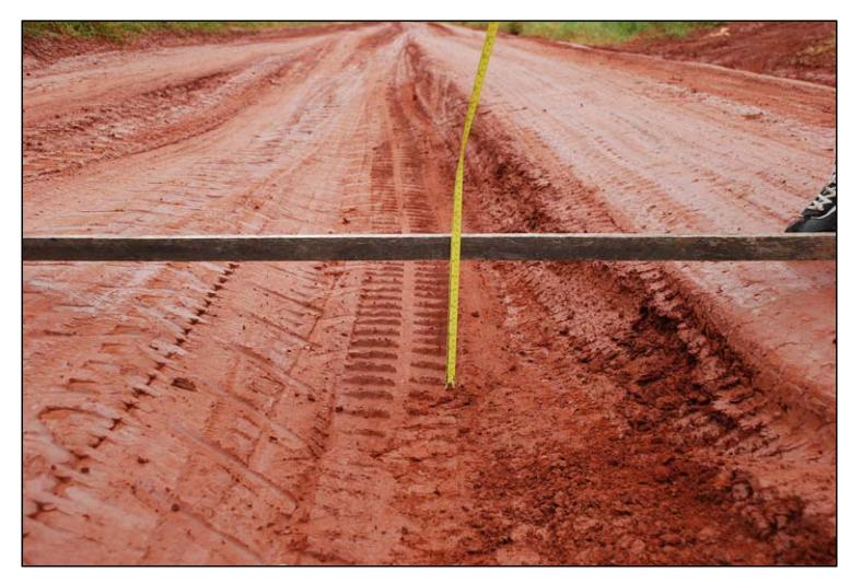
**Figure E.4.2 Severe Rutting in Road 2.1**
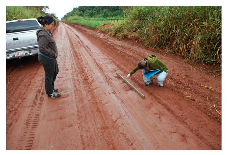
**Figure E.4.3 Fixed corrugations in Road 9**
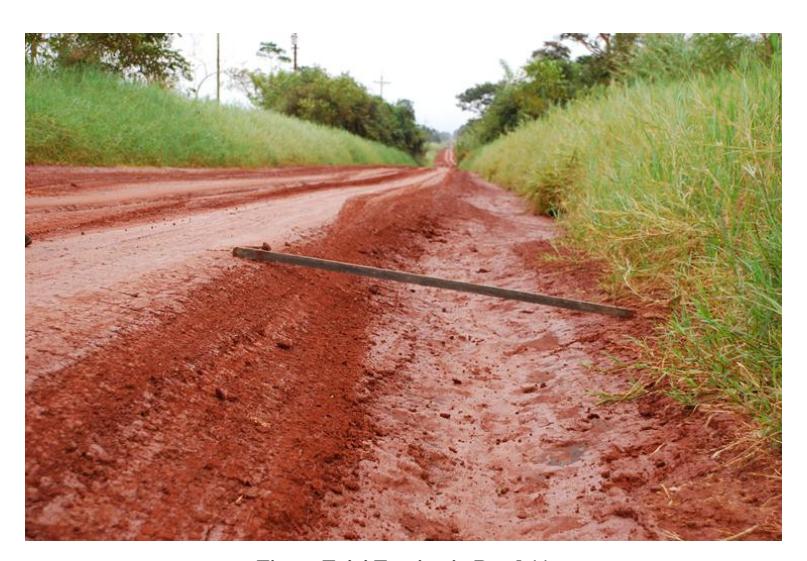
**Figure E.4.4 Erosion in Road 11**
**Appendix F Data Analysis: Development of Condition Performance Module**
### **F.1. Unpaved Roads Condition Index Validation**
| | Road Characteristics | | UPCI Values (1 to 10) | |
|--------------|----------------------|-----------------|-----------------------|----------|
| Section Code | Road Name | Road Length (m) | Calculated | Observed |
| 1 | V_LLA | 550 | 7.7 | 6.5 |
| 2 | N620 | 13900 | 6.2 | 6 |
| 3 | N496_R | 2000 | 2.8 | 3 |
| 4 | N496_T | 2800 | 6.3 | 6 |
| 6 | V_CU1 | 400 | 6.8 | 7.5 |
| 7 | V_CU2 | 500 | 6.5 | 5 |
| 8 | N600 | 9700 | 5.7 | 8 |
| 9 | N498 | 2000 | 7.3 | 6.5 |
| 10 | V_BQH | 850 | 4.0 | 4 |
| 11 | N474 | 5000 | 4.0 | 3 |
| 13 | V_BA2 | 1800 | 4.3 | 5 |
| 14 | N490 | 4000 | 6.2 | 7 |
| 15 | N480 | 7700 | 6.5 | 7 |
| 16 | N462 | 3300 | 4.2 | 6 |
| 17 | V_BAB | 1100 | 6.2 | 6 |
| 18 | V_CAB | 1700 | 3.7 | 3 |
| 19 | N616 | 3200 | 9.0 | 8 |
| 20 | N486 | 5800 | 7.6 | 7 |
| 21 | N466 | 11700 | 5.5 | 7 |
| 22 | N492 | 6800 | 7.2 | 7 |
| 25 | V_LNJ | 1200 | 3.8 | 6.5 |
| 26 | N482 | 11200 | 6.5 | 6 |
| 27 | N500 | 3000 | 6.4 | 5 |
| 28 | N478 | 5300 | 5.8 | 7 |
| 29 | V_PSA | 1300 | 5.8 | 6 |
| 30 | V_CHU | 3000 | 5.0 | 6 |
| 31 | V_AMI | 2000 | 4.1 | 5 |
| 32 | N494 | 5400 | 3.3 | 6 |
| 33 | V_LPL | 1600 | 6.4 | 7 |
| 34 | N610 | 10200 | 6.5 | 8 |
| 37 | N60-R | 15900 | 5.5 | 6.5 |
| 39 | N68 | 11000 | 8.8 | 8 |
#### **Statistical Analysis for UPCI Validation**
Analysis method: t Test of comparison of means
| | UPCI Calculated | UPCI Observed |
|---------------------------------|-----------------|---------------|
| Mean | 5.88 | 6.11 |
| Variance | 2.23 | 2.03 |
| Observations | 31 | 31 |
| Pearson Correlation Coefficient | 0.72 | |
| Difference between means | 0 | |
| Degrees of Freedom | 30 | |
| t observed | -1.19 | |
| P(T<=t) two tailed test | 0.24 | |
| t critical (two tailed test) | 2.04 | |
1. Null Hypothesis H0 : µ1 - µ2 = 0
2. Alternative Hypothesis H01 : µ1 - µ2 ≠ 0
3. Significance Level α=0.05
4. Comparison of test statistic to critical value and decide:
The null hypothesis is rejected when tcritical < t or when t < - tcritical
tcritical = 2.04 > t = -1.19 > - tcritical = - 2.04
We fail to reject the null hypothesis and therefore state that both means are equal with a confidence of 95%

### **F.2. Maintenance Effects on Roads Condition**
#### **F.2.1 Analysis Statistics for Gravel Roads**
| | Summer | | | | | | | | | | | | |
|---------|------------------|-----------------|------------|------------------|-----------------|---------------|--|--|--|--|--|--|--|
| Grading | Pre Maint
Dry | Abs Dry
Incr | % Dry Incr | Pre Maint
Med | Abs Med
Incr | % Med
Incr | | | | | | | |
| Min | 6.02 | 2.40 | 34% | 6.02 | 3.63 | 57% | | | | | | | |
| Max | 7.15 | 3.35 | 56% | 6.37 | 3.98 | 66% | | | | | | | |
| Mean | 6.59 | 2.87 | 45% | 6.20 | 3.80 | 61% | | | | | | | |
| SD | 0.80 | 0.67 | 16% | 0.25 | 0.25 | 6% | | | | | | | |
| | Summer | | | | | | | | | | | | |
|---------------------------|------------------|-----------------|------------|------------------|-----------------|---------------|--|--|--|--|--|--|--|
| Local Gravel +
Grading | Pre Maint
Dry | Abs Dry
Incr | % Dry Incr | Pre Maint
Med | Abs Med
Incr | % Med
Incr | | | | | | | |
| Min | 3.50 | 0.83 | 9% | 3.50 | 1.17 | 13% | | | | | | | |
| Max | 9.17 | 6.50 | 186% | 8.83 | 6.50 | 186% | | | | | | | |
| Mean | 6.59 | 3.18 | 64% | 6.44 | 3.39 | 68% | | | | | | | |
| SD | 2.03 | 2.07 | 69% | 1.95 | 1.93 | 68% | | | | | | | |
| | | | Summer | | | |
|------------------------------------|------------------|-----------------|------------|------------------|-----------------|---------------|
| Culvert replacement
and grading | Pre Maint
Dry | Abs Dry
Incr | % Dry Incr | Pre Maint
Med | Abs Med
Incr | % Med
Incr |
| Mean (1 obs) | 4.54 | 1.13 | 0.25 | 4.52 | 1.15 | 0.26 |
| | | | Winter | | | |
|---------|---------------------|--------------------|---------------|-----------------------|-------------------|-----------------|
| Grading | Pre
Maint
Med | Abs
Med
Incr | % Med
Incr | Pre
Maint
Humid | Abs Humid
Incr | % Humid
Incr |
| Min | 2.30 | 2.57 | 74% | 2.30 | 2.57 | 82% |
| Max | 4.73 | 3.52 | 112% | 4.73 | 3.89 | 112% |
| Mean | 3.52 | 3.04 | 93% | 3.52 | 3.23 | 97% |
| SD | 1.72 | 0.67 | 26% | 1.72 | 0.94 | 21% |
| | | | Winter | | | |
|---------------------------|---------------------|--------------------|---------------|-----------------------|-------------------|-----------------|
| Local Gravel +
Grading | Pre
Maint
Med | Abs
Med
Incr | % Med
Incr | Pre
Maint
Humid | Abs Humid
Incr | % Humid
Incr |
| Min | 5.33 | 0.06 | 1% | 5.33 | 0.93 | 12% |
| Max | 8.10 | 4.67 | 88% | 8.10 | 4.67 | 88% |
| Mean | 7.13 | 1.51 | 26% | 7.13 | 2.39 | 38% |
| SD | 1.23 | 2.13 | 41% | 1.23 | 1.62 | 34% |
| Winter | | | | | | | | |
|------------------------------|---------------------|--------------------|---------------|-----------------------|-------------------|-----------------|--|--|
| Bridge repair and
grading | Pre
Maint
Med | Abs
Med
Incr | % Med
Incr | Pre
Maint
Humid | Abs Humid
Incr | % Humid
Incr | | |
| Mean (1 obs) | 6.91 | 1.34 | 19% | 6.58 | 2.04 | 31% | | |
| | Winter | | | | | | | | |
|--------------|---------------------|--------------------|---------------|-----------------------|-------------------|-----------------|--|--|--|
| Local gravel | Pre
Maint
Med | Abs
Med
Incr | % Med
Incr | Pre
Maint
Humid | Abs Humid
Incr | % Humid
Incr | | | |
| Min | 4.30 | 0.58 | 6% | 4.30 | 0.71 | 8% | | | |
| Max | 9.42 | 3.37 | 78% | 9.29 | 3.62 | 84% | | | |
| Mean | 6.86 | 1.98 | 42% | 6.80 | 2.16 | 46% | | | |
| SD | 3.62 | 1.97 | 51% | 3.53 | 2.06 | 54% | | | |
#### **F.2.2 Analysis Statistics for Earth Roads**
| Summer | | | | | | | | |
|----------------------|------------------|-----------------|------------|------------------|-----------------|---------------|--|--|
| 1 Grading
(7 obs) | Pre Maint
Dry | Abs Dry
Incr | % Dry Incr | Pre Maint
Med | Abs Med
Incr | % Med
Incr | | |
| Min | 2.75 | 1.50 | 28% | 2.78 | 2.38 | 63% | | |
| Max | 5.40 | 7.25 | 264% | 5.20 | 7.22 | 260% | | |
| Mean | 4.03 | 3.52 | 99% | 3.94 | 4.33 | 119% | | |
| SD | 1.11 | 1.94 | 78% | 1.04 | 1.53 | 67% | | |
| Summer | | | | | | | | | |
|-----------------------|------------------|-----------------|------------|------------------|-----------------|---------------|--|--|--|
| 2 Gradings (3
obs) | Pre Maint
Dry | Abs Dry
Incr | % Dry Incr | Pre Maint
Med | Abs Med
Incr | % Med
Incr | | | |
| Min | 3.34 | 2.67 | 73% | 3.29 | 2.69 | 74% | | | |
| Max | 3.93 | 4.72 | 120% | 3.91 | 4.74 | 136% | | | |
| Mean | 3.65 | 3.72 | 102% | 3.61 | 3.96 | 110% | | | |
| SD | 0.30 | 1.03 | 26% | 0.31 | 1.11 | 32% | | | |
| Summer | | | | | | | |
|----------------------------------|------------------|-----------------|------------|------------------|-----------------|---------------|--|
| 1 Culvert
repair+1
grading | Pre Maint
Dry | Abs Dry
Incr | % Dry Incr | Pre Maint
Med | Abs Med
Incr | % Med
Incr | |
| Mean (1 obs) | 3.25 | 6.33 | 195% | 3.20 | 6.70 | 209% | |
| Summer | | | | | | | |
|-------------------------------|------------------|-----------------|------------|------------------|-----------------|---------------|--|
| 1 local gravel +
1 grading | Pre Maint
Dry | Abs Dry
Incr | % Dry Incr | Pre Maint
Med | Abs Med
Incr | % Med
Incr | |
| Mean (1 obs) | 2.29 | 5.56 | 243% | 2.27 | 7.38 | 325% | |
| Winter | | | | | | | | | |
|-------------------|----|---------------------|--------------------|---------------|-----------------------|-------------------|-----------------|--|--|
| 1 Grading
obs) | (2 | Pre
Maint
Med | Abs
Med
Incr | % Med
Incr | Pre
Maint
Humid | Abs Humid
Incr | % Humid
Incr | | |
| Min | | 3.91 | 1.45 | 18% | 3.79 | 1.45 | 18% | | |
| Max | | 7.92 | 3.87 | 99% | 7.92 | 4.11 | 108% | | |
| Mean | | 5.92 | 2.66 | 59% | 5.86 | 2.78 | 63% | | |
| SD | | 2.84 | 1.71 | 57% | 2.92 | 1.88 | 64% | | |
| Winter | | | | | | | | | |
|--------------------|----|---------------------|--------------------|---------------|-----------------------|-------------------|-----------------|--|--|
| 2 Gradings
obs) | (3 | Pre
Maint
Med | Abs
Med
Incr | % Med
Incr | Pre
Maint
Humid | Abs Humid
Incr | % Humid
Incr | | |
| Min | | 3.67 | 2.69 | 66% | 3.62 | 2.72 | 68% | | |
| Max | | 4.70 | 3.55 | 90% | 4.70 | 3.65 | 95% | | |
| Mean | | 4.10 | 3.12 | 77% | 4.06 | 3.18 | 79% | | |
| SD | | 0.53 | 0.43 | 12% | 0.57 | 0.47 | 14% | | |
| Winter | | | | | | | |
|-------------------------------|---------------------|--------------------|---------------|-----------------------|-------------------|-----------------|--|
| 1 Culvert
repair+1 grading | Pre
Maint
Med | Abs
Med
Incr | % Med
Incr | Pre
Maint
Humid | Abs Humid
Incr | % Humid
Incr | |
| Mean (1 obs) | 3.91 | 0.64 | 16% | 3.70 | 0.90 | 24% | |
| Winter | | | | | | | |
|-------------------------------|---------------------|--------------------|---------------|-----------------------|-------------------|-----------------|--|
| 2 local gravel + 1
grading | Pre
Maint
Med | Abs
Med
Incr | % Med
Incr | Pre
Maint
Humid | Abs Humid
Incr | % Humid
Incr | |
| Mean (1 obs) | 6.20 | 2.75 | 44% | 6.20 | 2.75 | 44% | |
| | Winter | | | | | | | | |
|----------------|---------------------|--------------------|---------------|-----------------------|-------------------|-----------------|--|--|--|
| 1 local gravel | Pre
Maint
Med | Abs
Med
Incr | % Med
Incr | Pre
Maint
Humid | Abs Humid
Incr | % Humid
Incr | | | |
| Min | 4.90 | 1.47 | 24% | 4.80 | 1.50 | 24% | | | |
| Max | 6.16 | 3.12 | 64% | 6.13 | 3.26 | 68% | | | |
| Mean | 5.53 | 2.30 | 44% | 5.47 | 2.38 | 46% | | | |
| SD | 0.89 | 1.17 | 28% | 0.94 | 1.24 | 31% | | | |
#### **F.3 Analysis of Maintenance Effects**
#### **F.3.1 Analysis of Maintenance Effects: Gravel Roads**
#### **Dry**
| | Overall Maint Abs. | | Application
Range |
|---------------------------------|--------------------|-----|----------------------|
| Maintenance | UPCI Incr | Min | Max |
| Grading | 2.9 | 6.0 | 7.2 |
| Local gravel + Grading | 3.2 | 3.5 | 9.2 |
| Culvert/Bridge Repair + Grading | 1.1 | | 4.5 |
#### **Mediterranean**
| | Overall Maint Abs. | Application Range | |
|---------------------------------|--------------------|-------------------|-----|
| Maintenance | UPCI Incr | Min | Max |
| Grading | 3.4 | 4.2 | 5.6 |
| Local gravel + Grading | 2.4 | 4.4 | 8.5 |
| Culvert/Bridge Repair + Grading | 1.2 | | 5.7 |
| Local Gravel | 2.0 | 4.3 | 9.4 |
#### **Humid**
| | Overall Maint | Application Range | | |
|---------------------------------------|-------------------|-------------------|-----|--|
| Maintenance | Abs. UPCI
Incr | Min | Max | |
| Grading | 3.2 | 2.3 | 4.7 | |
| Local gravel +
Grading | 2.4 | 5.3 | 8.1 | |
| Culvert/Bridge
Repair +
Grading | 2.0 | | 6.6 | |
| Local Gravel | 2.2 | 4.3 | 9.3 | |
#### **F.3.2 Analysis of Maintenance Effects: Earth Roads**
#### **Dry**
| | Overall Maint Abs. | | Application
Range |
|--------------------------------|--------------------|------|----------------------|
| Maintenance | UPCI Incr | Min | Max |
| Local Gravel/ Pothole Patching | | | |
| One Grading | 3.5 | 2.75 | 5.40 |
| Two Gradings | 3.7 | 3.34 | 3.93 |
| Culvert Repair + One Grading | 6.3 | 3.25 | |
| Local gravel + Grading | 5.6 | 2.29 | |
#### **Mediterranean**
| | Overall Maint Abs. | Application
Range | |
|--------------------------------|--------------------|----------------------|------|
| Maintenance | UPCI Incr | Min | Max |
| Local Gravel/ Pothole Patching | 2.3 | 4.90 | 6.16 |
| One Grading | 3.5 | 3.48 | 4.31 |
| Two Gradings | 3.5 | 3.48 | 4.31 |
| Culvert Repair + Grading | 3.7 | 3.56 | |
| Local Gravel+ Grading | 5.1 | 4.24 | |
#### **Humid**
| | Overall Maint Abs. | | Application
Range |
|-----------------------------------|--------------------|------|----------------------|
| Maintenance | UPCI Incr | Min | Max |
| Local Gravel/ Pothole
Patching | 2.4 | 4.80 | 6.13 |
| One Grading | 2.8 | 3.79 | 7.92 |
| Two Gradings | 3.2 | 3.62 | 0.95 |
| Culvert Repair + One
Grading | 0.9 | 3.70 | |
| Local Gravel+ One Grading | 2.8 | 6.20 | |
#### **F.4. Validation of Performance Curves and Maintenance Effects on Roads Condition F.4.1 Gravel Roads Validations**
| | Road Information | | | Traffic Data | | oct-11 |
|----|------------------|----------------|-----------------|------------------|------------------|-----------------|
| N° | Code | Road
length | Traffic
AADT | Traffic
level | UPCI
Observed | UPCI Calculated |
| 2 | N620 | 6900 | 100 | Moderate | 8.3 | 8.16 |
| 3 | N496_R | 2000 | 30 | Low | 6.1 | 6.78 |
| 8 | N600 | 9700 | 70 | Moderate | 9.5 | 7.43 |
| 14 | N490 | 4000 | 50 | Low | 7.7 | 7.5 |
| 15 | N480 | 7700 | 100 | Moderate | 7.1 | 7.83 |
| 16 | N462 | 3300 | 30 | Low | 3.4 | 3.83 |
| 19 | N616 | 3200 | 20 | Low | 8.3 | 6.15 |
| 20 | N486 | 5800 | 40 | Low | 7.7 | 8.15 |
| 21 | N466 | 11700 | 80 | Moderate | 9.5 | 8.92 |
| 26 | N482 | 10400 | 60 | Moderate | 8.4 | 8.33 |
| 27 | N500 | 3000 | 20 | Low | 8.9 | 8.32 |
| 28 | N478 | 5300 | 80 | Moderate | 7.0 | 6.32 |
| 34 | N610 | 10200 | 60 | Moderate | 5.0 | 5.5 |
| 36 | N510 | 4900 | 40 | Low | 9.2 | 8 |
| 37 | N60-R | 15900 | 220 | High | 6.2 | 6.42 |
| 39 | N68 | | 100 | Moderate | 6.3 | 6 |
#### **t-test for difference in means**
| | UPCI Observed | UPCI Calculated |
|---------------------------------|---------------|-----------------|
| Mean | 7.41 | 7.10 |
| Variance | 2.90 | 1.78 |
| Observations | 16 | 16 |
| Pearson Correlation Coefficient | 0.86 | |
| Difference between means | 0 | |
| Degrees of Freedom | 15 | |
| t observed | 1.41 | |
| P(T<=t) two tailed test | 0.18 | |
| t critical (two tailed test) | 2.13 | |
1. Null Hypothesis H0 : µ1 - µ2 = 0 2. Alternative Hypothesis H1 : µ1 - µ2 ≠ 0
3. Significance Level α=0.05 4. Comparison of test statistic to critical value and decide:
The null hypothesis is rejected when tcritical < t or when t < - tcritical
tcritical = 2.13 > t = 1.41 > - tcritical = - 2.13
We fail to reject the null hypothesis and therefore state that both means are equal with a confidence of 95%
**F.4.2. Earth Roads Validation**
| | Road Information | | | Traffic Data | | oct-11 |
|----|------------------|----------------|-----------------|------------------|------------------|-----------------|
| N° | Code | Road
length | Traffic
AADT | Traffic
level | UPCI
Observed | UPCI Calculated |
| 1 | V_LLA | 550 | 4 | Low | 4.9 | 4.56 |
| 4 | N496_T | 2800 | 6 | Low | 7.1 | 6.99 |
| 5 | V_QTA | 1400 | 14 | Low | 2.1 | 3 |
| 6 | V_CU1 | 400 | 10 | Low | 7.6 | 7.02 |
| 7 | V_CU2 | 500 | 10 | Low | 6.7 | 5.51 |
| 9 | N498 | 2000 | 14 | Low | 7.7 | 8.04 |
| 10 | V_BQH | 850 | 8 | Low | 4.4 | 4.4 |
| 11 | N474 | 5000 | 12 | Low | 5.4 | 5.4 |
| 17 | V_BAB | 1100 | 6 | Low | 5.6 | 4.49 |
| 18 | V_CAB | 1700 | 6 | Low | 5.8 | 4.06 |
| 22 | N492 | 6800 | 40 | Low | 7.1 | 7.03 |
| 25 | V_LNJ | 1200 | 16 | Low | 7.6 | 5.19 |
| 30 | V_CHU | 3000 | 30 | Low | 9.2 | 8.94 |
| 31 | V_AMI | 2000 | 6 | Low | 6.3 | 5.41 |
| 32 | N494 | 5400 | 60 | Moderate | 6.2 | 7.2 |
| 33 | V_LPL | 1600 | 30 | Low | 6.7 | 5.5 |
t-test for difference in means
| | UPCI Observed | UPCI Calculated |
|---------------------------------|---------------|-----------------|
| Mean | 6.26 | 5.80 |
| Variance | 2.65 | 2.55 |
| Observations | 16 | 16 |
| Pearson Correlation Coefficient | 0.84 | |
| Difference between means | 0 | |
| Degrees of Freedom | 15 | |
| t observed | 2.03 | |
| P(T<=t) two tailed test | 0.06 | |
| t critical (two tailed test) | 2.13 | |
1. Null Hypothesis H0 : µ1 - µ2 = 0 2. Alternative Hypothesis H1 : µ1 - µ2 ≠ 0 3. Significance Level α=0.05
4. Comparison of test statistic to critical value and decide:
The null hypothesis is rejected when tcritical < t or when t < - tcritical
tcritical = 2.13 > t = 2.03 > - tcritical = - 2.13
We fail to reject the null hypothesis and therefore state that both means are equal with a confidence of 95%
# **Appendix G**
# **Data Analysis: Development of Network Maintenance Module**
#### **G.1 Effectiveness Calculations for Gravel Roads**
Maintenance types applied in the analysis are: Minimum (Green), Routine (Purple), Rehabilitation (Blue), Reconstruction (Orange)
**G.1.1 Effectiveness for GRM1 Strategy**
| | | | | | Dry Climate | | | | |
|---------------------------|------------------|-------------|---------------|----------------|---------------|----------------|---------------|----------------|---------------|
| | | Min Budget | | | Low Budget | Med. Budget | | High Budget | |
| Maintenance | Cycle* | UPCI Before | UPCI
After | UPCI
Before | UPCI
After | UPCI
Before | UPCI
After | UPCI
Before | UPCI
After |
| | 0 | | 10 | | 10 | | 10 | | 10 |
| | 1 | 7.50 | 8.00 | 7.50 | 8.25 | 7.50 | 9.25 | 7.50 | 9.50 |
| | 2 | 6.70 | 7.65 | 6.80 | 8.23 | 7.20 | 9.25 | 7.30 | 9.50 |
| | 3 | 6.56 | 7.46 | 6.79 | 8.14 | 7.20 | 9.25 | 7.30 | 9.50 |
| | 4 | 6.47 | 7.32 | 6.76 | 8.03 | 7.20 | 9.25 | 7.30 | 9.50 |
| | 5 | 6.35 | 7.15 | 6.71 | 7.91 | 7.20 | 9.20 | 7.30 | 9.50 |
| | 6 | 6.21 | 6.96 | 6.66 | 7.79 | 7.18 | 9.06 | 7.30 | 9.50 |
| Prev: Local | 7 | 6.05 | 6.75 | 6.62 | 7.67 | 7.12 | 8.87 | 7.30 | 9.40 |
| Regravel+Min
Grading. | 8 | 5.87 | 6.52 | 6.57 | 7.54 | 7.05 | 8.67 | 7.26 | 9.21 |
| Rehab: | 9 | 5.69 | 6.29 | 6.52 | 7.42 | 6.97 | 8.47 | 7.18 | 8.98 |
| Grading+
Gravel / Rec: | 10 | 5.62 | 6.17 | 6.43 | 7.26 | 6.89 | 8.26 | 7.09 | 8.74 |
| Grading+ | 11 | 5.60 | 6.10 | 6.30 | 7.05 | 6.81 | 8.06 | 7.00 | 8.50 |
| Gravel+
Culvert | 12 | 5.59 | 6.04 | 6.12 | 6.80 | 6.72 | 7.85 | 6.90 | 8.25 |
| Replace. | 13 | 5.57 | 5.97 | 5.91 | 6.51 | 6.64 | 7.64 | 6.80 | 8.00 |
| | 14 | 5.56 | 5.91 | 5.68 | 6.20 | 6.56 | 7.43 | 6.70 | 7.75 |
| | 15 | 5.55 | 5.85 | 5.61 | 6.06 | 6.44 | 7.19 | 6.60 | 7.50 |
| | 16 | 5.54 | 5.79 | 5.58 | 5.95 | 6.24 | 6.87 | 6.50 | 7.25 |
| | 17 | 5.52 | 5.72 | 5.56 | 5.86 | 5.97 | 6.47 | 6.29 | 6.89 |
| | 18 | 5.51 | 5.66 | 5.54 | 5.76 | 5.66 | 6.04 | 5.99 | 6.44 |
| | 19 | 5.49 | 8.75 | 5.52 | 5.67 | 5.57 | 5.82 | 5.66 | 5.96 |
| | 20 | 7.00 | | 5.50 | | 5.53 | | 5.56 | |
| | Mean UPCI | 6.40 | | | 6.72 | 7.41 | | 7.67 | |
| | Unit Effective.* | 48.00 | | | 54.38 | 68.28 | | 73.35 | |
\*Min acceptable UPCI=4
#### **G.1.1 Effectiveness for GRM1 Strategy (cont.)**
| | | | | | Mediterranean Climate | | | | |
|---------------------------|------------------|----------------|---------------|-------------|-----------------------|----------------|---------------|----------------|---------------|
| | | | Min Budget | Low Budget | | Med. Budget | | High Budget | |
| Maintenance | Cycle* | UPCI
Before | UPCI
After | UPCI Before | UPCI After | UPCI
Before | UPCI
After | UPCI
Before | UPCI
After |
| | 0 | | 10 | | 10 | | 10 | | 10 |
| | 1 | 6.50 | 7.50 | 6.50 | 8.00 | 6.50 | 9.00 | 6.50 | 9.50 |
| | 2 | 5.90 | 6.85 | 6.02 | 7.45 | 6.26 | 8.64 | 6.38 | 9.23 |
| | 3 | 5.75 | 6.65 | 5.89 | 7.24 | 6.18 | 8.43 | 6.32 | 9.02 |
| | 4 | 5.70 | 6.55 | 5.84 | 7.12 | 6.13 | 8.25 | 6.27 | 8.82 |
| | 5 | 5.68 | 6.48 | 5.81 | 7.01 | 6.08 | 8.08 | 6.22 | 8.62 |
| | 6 | 5.66 | 6.41 | 5.79 | 6.91 | 6.04 | 7.92 | 6.17 | 8.42 |
| Prev: Local | 7 | 5.65 | 6.35 | 5.77 | 6.82 | 6.00 | 7.75 | 6.12 | 8.22 |
| Regravel+Min
Grading. | 8 | 5.64 | 6.29 | 5.74 | 6.72 | 5.97 | 7.59 | 6.08 | 8.03 |
| Rehab: | 9 | 5.62 | 6.22 | 5.72 | 6.62 | 5.93 | 7.43 | 6.03 | 7.83 |
| Grading+
Gravel / Rec: | 10 | 5.61 | 6.16 | 5.69 | 6.52 | 5.89 | 7.26 | 5.98 | 7.63 |
| Grading+ | 11 | 5.60 | 6.10 | 5.67 | 6.42 | 5.85 | 7.10 | 5.94 | 7.44 |
| Gravel+
Culvert | 12 | 5.59 | 6.04 | 5.65 | 6.33 | 5.81 | 6.93 | 5.89 | 7.24 |
| Replace. | 13 | 5.57 | 5.97 | 5.63 | 6.23 | 5.77 | 6.77 | 5.84 | 7.04 |
| | 14 | 5.56 | 5.91 | 5.61 | 6.14 | 5.73 | 6.61 | 5.80 | 6.85 |
| | 15 | 5.55 | 5.85 | 5.59 | 6.04 | 5.69 | 6.44 | 5.75 | 6.65 |
| | 16 | 5.54 | 5.79 | 5.58 | 5.95 | 5.66 | 6.28 | 5.70 | 6.45 |
| | 17 | 5.52 | 5.72 | 5.56 | 5.86 | 5.62 | 6.12 | 5.66 | 6.26 |
| | 18 | 5.51 | 5.66 | 5.54 | 5.76 | 5.59 | 5.97 | 5.62 | 6.07 |
| | 19 | 5.47 | 8.75 | 5.52 | 5.67 | 5.56 | 5.81 | 5.58 | 5.88 |
| | 20 | 6.20 | | 5.50 | | 5.53 | | 5.54 | |
| | Mean UPCI | | 6.13 | 6.24 | | 6.65 | | 6.86 | |
| | Unit Effective.* | | 42.55 | 124.72 | | 133.08 | | 137.29 | |
\*Min acceptable UPCI=4
#### **G.1.1 Effectiveness for GRM1 Strategy (cont.)**
| | | | | | | Humid Climate | | | |
|---------------------------|------------------|----------------|---------------|----------------|---------------|----------------|---------------|----------------|---------------|
| | | Min Budget | | | Low Budget | | Med. Budget | | High Budget |
| Maintenance | Cycle* | UPCI
Before | UPCI
After | UPCI
Before | UPCI
After | UPCI
Before | UPCI
After | UPCI
Before | UPCI
After |
| | 0 | | 10 | | 10 | | 10 | | 10 |
| | 1 | 5.75 | 6.75 | 5.75 | 7.25 | 5.75 | 8.25 | 5.75 | 8.75 |
| | 2 | 5.56 | 6.51 | 5.59 | 7.01 | 5.65 | 8.02 | 5.68 | 8.53 |
| | 3 | 5.54 | 6.44 | 5.57 | 6.92 | 5.63 | 7.88 | 5.66 | 8.36 |
| | 4 | 5.54 | 6.39 | 5.57 | 6.84 | 5.63 | 7.75 | 5.65 | 8.20 |
| | 5 | 5.54 | 6.34 | 5.56 | 6.76 | 5.62 | 7.62 | 5.64 | 8.04 |
| | 6 | 5.53 | 6.28 | 5.56 | 6.68 | 5.61 | 7.48 | 5.63 | 7.88 |
| Prev: Local | 7 | 5.53 | 6.23 | 5.55 | 6.60 | 5.60 | 7.35 | 5.63 | 7.73 |
| Regravel+Min
Grading. | 8 | 5.53 | 6.18 | 5.55 | 6.53 | 5.59 | 7.22 | 5.62 | 7.57 |
| Rehab: | 9 | 5.53 | 6.13 | 5.55 | 6.45 | 5.59 | 7.09 | 5.61 | 7.41 |
| Grading+
Gravel / Rec: | 10 | 5.52 | 6.07 | 5.54 | 6.37 | 5.58 | 6.95 | 5.60 | 7.25 |
| Grading+ | 11 | 5.52 | 6.02 | 5.54 | 6.29 | 5.57 | 6.82 | 5.59 | 7.09 |
| Gravel+
Culvert | 12 | 5.52 | 5.97 | 5.53 | 6.21 | 5.56 | 6.69 | 5.58 | 6.93 |
| Replace. | 13 | 5.51 | 5.91 | 5.53 | 6.13 | 5.56 | 6.56 | 5.57 | 6.77 |
| | 14 | 5.51 | 5.86 | 5.52 | 6.05 | 5.55 | 6.42 | 5.56 | 6.61 |
| | 15 | 5.51 | 5.81 | 5.52 | 5.97 | 5.54 | 6.29 | 5.55 | 6.45 |
| | 16 | 5.50 | 8.75 | 5.51 | 5.89 | 5.53 | 6.16 | 5.54 | 6.29 |
| | 17 | 5.68 | 6.68 | 5.51 | 5.81 | 5.52 | 6.02 | 5.53 | 6.13 |
| | 18 | 5.55 | 6.50 | 5.50 | 8.75 | 5.52 | 5.89 | 5.52 | 5.97 |
| | 19 | 5.54 | 6.44 | 5.68 | 7.18 | 5.51 | 5.76 | 5.51 | 5.81 |
| | 20 | 5.54 | | 5.58 | | 5.50 | | 5.50 | |
| | Mean UPCI | 6.06 | | | 6.17 | | 6.35 | | 6.49 |
| | Unit Effective.* | 41.11 | | | 123.45 | | 126.91 | | 129.85 |
#### **G.1.2 Effectiveness for GRM2 Strategy**
| | | | | | Dry Climate | | | | |
|---------------------------------------|------------------|-------------|---------------|----------------|---------------|----------------|---------------|----------------|---------------|
| | | Min Budget | | | Low Budget | Med. Budget | | High Budget | |
| Maintenance | Cycle* | UPCI Before | UPCI
After | UPCI
Before | UPCI
After | UPCI
Before | UPCI
After | UPCI
Before | UPCI
After |
| | 0 | | 10 | | 10 | | 10 | | 10 |
| | 1 | 7.50 | 8.00 | 7.50 | 8.25 | 7.50 | 9.25 | 7.50 | 9.50 |
| | 2 | 6.70 | 7.65 | 6.80 | 8.25 | 7.20 | 9.25 | 7.30 | 9.50 |
| | 3 | 6.56 | 7.46 | 6.80 | 8.25 | 7.20 | 9.25 | 7.30 | 9.50 |
| | 4 | 6.47 | 7.32 | 6.80 | 8.25 | 7.20 | 9.25 | 7.30 | 9.50 |
| | 5 | 6.35 | 7.15 | 6.80 | 8.25 | 7.20 | 9.25 | 7.30 | 9.50 |
| | 6 | 6.21 | 6.96 | 6.80 | 8.25 | 7.20 | 9.25 | 7.30 | 9.50 |
| | 7 | 6.05 | 6.75 | 6.80 | 8.25 | 7.20 | 9.25 | 7.30 | 9.50 |
| Prev: Routine | 8 | 5.87 | 6.52 | 6.80 | 8.25 | 7.20 | 9.25 | 7.30 | 9.50 |
| Grading. Rehab: | 9 | 5.69 | 6.29 | 6.80 | 8.25 | 7.20 | 9.25 | 7.30 | 9.50 |
| Grading+ Gravel.
Rec: | 10 | 5.62 | 6.17 | 6.80 | 8.18 | 7.20 | 9.13 | 7.30 | 9.50 |
| Grading+Regravel+
Culvert Replace. | 11 | 5.60 | 6.10 | 6.77 | 8.02 | 7.15 | 8.90 | 7.30 | 9.30 |
| | 12 | 5.59 | 6.04 | 6.71 | 7.83 | 7.06 | 8.64 | 7.22 | 9.02 |
| | 13 | 5.57 | 5.97 | 6.63 | 7.63 | 6.95 | 8.35 | 7.11 | 8.71 |
| | 14 | 5.56 | 5.91 | 6.55 | 7.43 | 6.84 | 8.07 | 6.98 | 8.38 |
| | 15 | 5.55 | 5.85 | 6.44 | 7.19 | 6.73 | 7.78 | 6.85 | 8.05 |
| | 16 | 5.54 | 5.79 | 6.24 | 6.87 | 6.61 | 7.49 | 6.72 | 7.72 |
| | 17 | 5.52 | 5.72 | 5.97 | 6.47 | 6.49 | 7.19 | 6.59 | 7.39 |
| | 18 | 5.51 | 5.66 | 5.66 | 6.04 | 6.24 | 6.77 | 6.41 | 7.01 |
| | 19 | 5.49 | 8.75 | 5.57 | 5.82 | 5.89 | 6.24 | 6.09 | 6.49 |
| | 20 | 7.00 | | 5.53 | | 5.61 | | 5.66 | |
| | Mean UPCI | 6.40 | | | 7.16 | 7.74 | | 7.93 | |
| | Unit Effective.* | 48.00 | | | 63.26 | 74.83 | | 78.60 | |
\*Min acceptable UPCI=4
#### **G.1.2 Effectiveness for GRM2 Strategy (cont.)**
| | | | | | Mediterranean Climate | | | | |
|---------------------------------------|------------------|----------------|------------|-------------|-----------------------|-------------|---------------|----------------|---------------|
| | | | Min Budget | Low Budget | | Med. Budget | | High Budget | |
| Maintenance | Cycle* | UPCI
Before | UPCI After | UPCI Before | UPCI After | UPCI Before | UPCI
After | UPCI
Before | UPCI
After |
| | 0 | | 10 | | 10 | | 10 | | 10 |
| | 1 | 6.50 | 7.50 | 6.50 | 8.25 | 6.50 | 9.25 | 6.50 | 9.50 |
| | 2 | 5.90 | 6.85 | 6.08 | 8.25 | 6.32 | 9.25 | 6.38 | 9.50 |
| | 3 | 5.75 | 6.65 | 6.08 | 8.25 | 6.32 | 9.25 | 6.38 | 9.50 |
| | 4 | 5.70 | 6.55 | 6.08 | 8.21 | 6.32 | 9.25 | 6.38 | 9.50 |
| | 5 | 5.68 | 6.48 | 6.07 | 8.07 | 6.32 | 9.12 | 6.38 | 9.50 |
| | 6 | 5.66 | 6.41 | 6.04 | 7.92 | 6.29 | 8.92 | 6.38 | 9.38 |
| | 7 | 5.65 | 6.35 | 6.00 | 7.75 | 6.24 | 8.69 | 6.35 | 9.15 |
| Prev: Routine | 8 | 5.64 | 6.29 | 5.97 | 7.59 | 6.19 | 8.46 | 6.30 | 8.90 |
| Grading. Rehab: | 9 | 5.62 | 6.22 | 5.93 | 7.43 | 6.13 | 8.23 | 6.24 | 8.64 |
| Grading+ Gravel.
Rec: | 10 | 5.61 | 6.16 | 5.89 | 7.26 | 6.08 | 8.00 | 6.18 | 8.38 |
| Grading+Regravel+
Culvert Replace. | 11 | 5.60 | 6.10 | 5.85 | 7.10 | 6.02 | 7.77 | 6.11 | 8.11 |
| | 12 | 5.59 | 6.04 | 5.81 | 6.93 | 5.97 | 7.55 | 6.05 | 7.85 |
| | 13 | 5.57 | 5.97 | 5.77 | 6.77 | 5.92 | 7.32 | 5.99 | 7.59 |
| | 14 | 5.56 | 5.91 | 5.73 | 6.61 | 5.86 | 7.09 | 5.93 | 7.33 |
| | 15 | 5.55 | 5.85 | 5.69 | 6.44 | 5.81 | 6.86 | 5.86 | 7.06 |
| | 16 | 5.54 | 5.79 | 5.66 | 6.28 | 5.75 | 6.63 | 5.80 | 6.80 |
| | 17 | 5.52 | 5.72 | 5.62 | 6.12 | 5.70 | 6.40 | 5.74 | 6.54 |
| | 18 | 5.51 | 5.66 | 5.59 | 5.97 | 5.65 | 6.17 | 5.68 | 6.28 |
| | 19 | 5.47 | 8.75 | 5.56 | 5.81 | 5.60 | 5.95 | 5.62 | 6.02 |
| | 20 | 6.20 | | 5.53 | | 5.56 | | 5.57 | |
| | Mean UPCI | | 6.13 | 6.61 | | 7.02 | | 7.18 | |
| | Unit Effective.* | | 42.55 | 132.23 | | 140.35 | | 143.67 | |
\*Min acceptable UPCI=4
#### **G.1.2 Effectiveness for GRM2 Strategy (cont.)**
| | | | | | | Humid Climate | | | |
|---------------------------------------|------------------|----------------|---------------|----------------|---------------|----------------|---------------|----------------|---------------|
| | | Min Budget | | | Low Budget | | Med. Budget | | High Budget |
| Maintenance | Cycle* | UPCI
Before | UPCI
After | UPCI
Before | UPCI
After | UPCI
Before | UPCI
After | UPCI
Before | UPCI
After |
| | 0 | | 10 | | 10 | | 10 | | 10 |
| | 1 | 5.75 | 6.75 | 5.75 | 8.25 | 5.75 | 9.25 | 5.75 | 9.50 |
| | 2 | 5.56 | 6.51 | 5.65 | 8.02 | 5.71 | 9.03 | 5.72 | 9.50 |
| | 3 | 5.54 | 6.44 | 5.63 | 7.88 | 5.69 | 8.84 | 5.72 | 9.32 |
| | 4 | 5.54 | 6.39 | 5.63 | 7.75 | 5.68 | 8.66 | 5.71 | 9.11 |
| | 5 | 5.54 | 6.34 | 5.62 | 7.62 | 5.67 | 8.47 | 5.70 | 8.90 |
| | 6 | 5.53 | 6.28 | 5.61 | 7.48 | 5.66 | 8.29 | 5.69 | 8.69 |
| | 7 | 5.53 | 6.23 | 5.60 | 7.35 | 5.65 | 8.10 | 5.67 | 8.47 |
| Prev: Routine | 8 | 5.53 | 6.18 | 5.59 | 7.22 | 5.64 | 7.91 | 5.66 | 8.26 |
| Grading. Rehab: | 9 | 5.53 | 6.13 | 5.59 | 7.09 | 5.63 | 7.73 | 5.65 | 8.05 |
| Grading+ Gravel.
Rec: | 10 | 5.52 | 6.07 | 5.58 | 6.95 | 5.62 | 7.54 | 5.64 | 7.84 |
| Grading+Regravel+
Culvert Replace. | 11 | 5.52 | 6.02 | 5.57 | 6.82 | 5.61 | 7.36 | 5.62 | 7.62 |
| | 12 | 5.52 | 5.97 | 5.56 | 6.69 | 5.59 | 7.17 | 5.61 | 7.41 |
| | 13 | 5.51 | 5.91 | 5.56 | 6.56 | 5.58 | 6.98 | 5.60 | 7.20 |
| | 14 | 5.51 | 5.86 | 5.55 | 6.42 | 5.57 | 6.80 | 5.59 | 6.99 |
| | 15 | 5.51 | 5.81 | 5.54 | 6.29 | 5.56 | 6.61 | 5.57 | 6.77 |
| | 16 | 5.50 | 8.75 | 5.53 | 6.16 | 5.55 | 6.43 | 5.56 | 6.56 |
| | 17 | 5.68 | 6.68 | 5.52 | 6.02 | 5.54 | 6.24 | 5.55 | 6.35 |
| | 18 | 5.55 | 6.50 | 5.52 | 5.89 | 5.53 | 6.05 | 5.54 | 6.14 |
| | 19 | 5.54 | 6.44 | 5.51 | 5.76 | 5.52 | 5.87 | 5.52 | 5.92 |
| | 20 | 5.54 | | 5.50 | | 5.51 | | 5.51 | |
| | Mean UPCI | 6.06 | | | 6.35 | | 6.64 | | 6.78 |
| | Unit Effective.* | 41.11 | | | 126.91 | | 132.79 | | 135.57 |
\*Min acceptable UPCI=4
#### **G.2 Effectiveness Calculations for Earth Roads**
Maintenance types applied in the analysis are: Minimum (Green), Routine (Purple), Rehabilitation (Blue), Reconstruction (Orange)
#### **G.2.1 Effectiveness for ERM1 Strategy**
| | | | | | Dry Climate | | | | |
|------------------------------------|------------------|-------------|---------------|----------------|---------------|----------------|---------------|----------------|---------------|
| | | Min Budget | | | Low Budget | Med. Budget | | High Budget | |
| Maintenance | Cycle* | UPCI Before | UPCI
After | UPCI
Before | UPCI
After | UPCI
Before | UPCI
After | UPCI
Before | UPCI
After |
| | 0 | | 10 | | 10 | | 10 | | 10 |
| | 1 | 7.50 | 8.00 | 7.50 | 8.25 | 7.50 | 9.25 | 7.50 | 9.50 |
| | 2 | 6.70 | 7.65 | 6.80 | 8.23 | 7.20 | 9.25 | 7.30 | 9.50 |
| | 3 | 6.56 | 7.46 | 6.79 | 8.14 | 7.20 | 9.25 | 7.30 | 9.50 |
| | 4 | 6.40 | 7.25 | 6.76 | 8.03 | 7.20 | 9.25 | 7.30 | 9.50 |
| | 5 | 5.86 | 6.66 | 6.71 | 7.91 | 7.20 | 9.20 | 7.30 | 9.50 |
| | 6 | 4.35 | 7.85 | 6.66 | 7.79 | 7.18 | 9.06 | 7.30 | 9.50 |
| | 7 | 6.64 | 7.64 | 6.62 | 7.67 | 7.12 | 8.87 | 7.30 | 9.40 |
| Prev: Local | 8 | 6.56 | 7.51 | 6.57 | 7.54 | 7.05 | 8.67 | 7.26 | 9.21 |
| Regravel+Min
Grading. Rehab: | 9 | 6.50 | 7.40 | 6.52 | 7.42 | 6.97 | 8.47 | 7.18 | 8.98 |
| Grading+ Gravel
/ Rec: Grading+ | 10 | 6.25 | 7.10 | 6.29 | 7.11 | 6.89 | 8.26 | 7.09 | 8.74 |
| Gravel+ Culvert | 11 | 5.48 | 8.75 | 5.51 | 6.26 | 6.81 | 8.06 | 7.00 | 8.50 |
| Replace. | 12 | 7.00 | 8.00 | 3.94 | 8.94 | 6.72 | 7.85 | 6.90 | 8.25 |
| | 13 | 6.70 | 7.65 | 7.08 | 8.25 | 6.64 | 7.64 | 6.80 | 8.00 |
| | 14 | 6.56 | 7.46 | 6.80 | 8.23 | 6.56 | 7.43 | 6.70 | 7.75 |
| | 15 | 6.40 | 7.25 | 6.79 | 8.14 | 6.32 | 7.07 | 6.60 | 7.50 |
| | 16 | 5.86 | 6.66 | 6.76 | 8.03 | 5.41 | 9.50 | 6.50 | 7.25 |
| | 17 | 4.35 | 7.85 | 6.71 | 7.91 | 7.30 | 9.25 | 5.86 | 6.46 |
| | 18 | 6.64 | 7.64 | 6.66 | 7.79 | 7.20 | 9.25 | 3.95 | 10.00 |
| | 19 | 6.56 | 7.51 | 6.62 | 7.67 | 7.20 | 9.25 | 7.50 | 9.50 |
| | 20 | 6.50 | | 6.57 | | 7.20 | | 7.30 | |
| | Mean UPCI | 6.97 | | | 7.25 | 7.84 | | 7.86 | |
| | Unit Effective.* | 59.30 | | | 64.97 | 76.84 | | 77.24 | |
\*Min acceptable UPCI=4
#### **G.2.1 Effectiveness for ERM1 Strategy (cont.)**
| | | | | | Mediterranean Climate | | | | |
|------------------------------------|------------------|----------------|------------|-------------|-----------------------|-------------|---------------|----------------|---------------|
| | | | Min Budget | Low Budget | | Med. Budget | | High Budget | |
| Maintenance | Cycle* | UPCI
Before | UPCI After | UPCI Before | UPCI After | UPCI Before | UPCI
After | UPCI
Before | UPCI
After |
| | 0 | | 10 | | 10 | | 10 | | 10 |
| | 1 | 7.50 | 8.00 | 7.50 | 8.25 | 7.50 | 9.25 | 7.50 | 9.50 |
| | 2 | 4.66 | 8.16 | 5.02 | 8.52 | 6.44 | 8.81 | 6.79 | 9.50 |
| | 3 | 4.89 | 8.39 | 5.39 | 8.75 | 5.81 | 8.06 | 6.79 | 9.49 |
| | 4 | 5.21 | 8.71 | 5.73 | 7.23 | 4.75 | 9.25 | 6.78 | 9.33 |
| | 5 | 5.67 | 6.67 | 3.94 | 8.94 | 6.43 | 8.93 | 6.54 | 8.94 |
| | 6 | 3.93 | 8.93 | 6.00 | 7.50 | 5.98 | 8.35 | 6.00 | 8.25 |
| | 7 | 5.98 | 6.98 | 3.95 | 8.95 | 5.16 | 9.50 | 5.01 | 9.75 |
| Prev: Local | 8 | 3.94 | 8.94 | 6.01 | 7.51 | 6.79 | 9.25 | 7.15 | 9.50 |
| Regravel+Min
Grading. Rehab: | 9 | 5.99 | 6.99 | 3.96 | 8.96 | 6.44 | 8.81 | 6.79 | 9.50 |
| Grading+ Gravel | 10 | 3.94 | 8.94 | 6.03 | 7.53 | 5.81 | 8.06 | 6.79 | 9.49 |
| / Rec: Grading+
Gravel+ Culvert | 11 | 5.99 | 6.99 | 3.99 | 8.99 | 4.75 | 9.25 | 6.78 | 9.33 |
| Replace. | 12 | 3.94 | 8.94 | 6.06 | 7.56 | 6.43 | 8.93 | 6.54 | 8.94 |
| | 13 | 5.99 | 6.99 | 4.04 | 7.54 | 5.98 | 8.35 | 6.00 | 8.25 |
| | 14 | 3.94 | 8.94 | 4.01 | 7.51 | 5.16 | 9.50 | 5.01 | 9.75 |
| | 15 | 5.99 | 6.99 | 3.96 | 8.96 | 6.79 | 9.25 | 7.15 | 9.50 |
| | 16 | 3.94 | 8.94 | 6.02 | 7.52 | 6.44 | 8.81 | 6.79 | 9.50 |
| | 17 | 5.99 | 6.99 | 3.98 | 8.98 | 5.81 | 8.06 | 6.79 | 9.49 |
| | 18 | 3.94 | 8.94 | 6.06 | 7.56 | 4.75 | 9.25 | 6.78 | 9.33 |
| | 19 | 5.99 | 6.99 | 4.03 | 7.53 | 6.43 | 8.93 | 6.54 | 8.94 |
| | 20 | 3.94 | | 3.99 | | 5.98 | | 6.00 | |
| | Mean UPCI | | 6.57 | 6.60 | | 7.45 | | 7.92 | |
| | Unit Effective.* | | 51.36 | 131.97 | | 149.09 | | 158.39 | |
\*Min acceptable UPCI=4
#### **G.2.1 Effectiveness for ERM1 Strategy (cont.)**
| | | | | | | Humid Climate | | | | |
|------------------------------------|------------------|----------------|---------------|----------------|---------------|----------------|---------------|----------------|---------------|--|
| | | Min Budget | | | Low Budget | | Med. Budget | High Budget | | |
| Maintenance | Cycle* | UPCI
Before | UPCI
After | UPCI
Before | UPCI
After | UPCI
Before | UPCI
After | UPCI
Before | UPCI
After | |
| | 0 | | 10 | | 10 | | 10 | | 10 | |
| | 1 | 7.50 | 8.00 | 7.50 | 8.25 | 7.50 | 9.25 | 7.50 | 9.50 | |
| | 2 | 4.60 | 8.10 | 4.96 | 8.46 | 6.41 | 8.79 | 6.78 | 9.50 | |
| | 3 | 4.74 | 8.24 | 5.27 | 8.75 | 5.74 | 7.99 | 6.78 | 9.48 | |
| | 4 | 4.96 | 8.46 | 5.69 | 7.19 | 4.59 | 9.09 | 6.74 | 9.29 | |
| | 5 | 5.26 | 8.75 | 3.86 | 8.86 | 6.18 | 8.68 | 6.47 | 8.87 | |
| | 6 | 5.69 | 6.69 | 5.84 | 7.34 | 5.58 | 7.96 | 5.86 | 8.11 | |
| | 7 | 3.83 | 8.83 | 3.87 | 8.87 | 4.54 | 9.04 | 4.76 | 9.75 | |
| Prev: Local | 8 | 5.80 | 6.80 | 5.86 | 7.36 | 6.11 | 8.61 | 7.14 | 9.50 | |
| Regravel+Min
Grading. Rehab: | 9 | 3.83 | 8.83 | 3.87 | 8.87 | 5.48 | 9.50 | 6.78 | 9.50 | |
| Grading+ Gravel | 10 | 5.81 | 6.81 | 5.86 | 7.36 | 6.78 | 9.25 | 6.78 | 9.48 | |
| / Rec: Grading+
Gravel+ Culvert | 11 | 3.84 | 8.84 | 3.87 | 8.87 | 6.41 | 8.79 | 6.74 | 9.29 | |
| Replace. | 12 | 5.81 | 6.81 | 5.86 | 7.36 | 5.74 | 7.99 | 6.47 | 8.87 | |
| | 13 | 3.84 | 8.84 | 3.87 | 8.87 | 4.59 | 9.09 | 5.86 | 8.11 | |
| | 14 | 5.81 | 6.81 | 5.86 | 7.36 | 6.18 | 8.68 | 4.76 | 9.75 | |
| | 15 | 3.84 | 8.84 | 3.87 | 8.87 | 5.58 | 7.96 | 7.14 | 9.50 | |
| | 16 | 5.81 | 6.81 | 5.86 | 7.36 | 4.54 | 9.04 | 6.78 | 9.50 | |
| | 17 | 3.84 | 8.84 | 3.87 | 8.87 | 6.11 | 8.61 | 6.78 | 9.48 | |
| | 18 | 5.81 | 6.81 | 5.86 | 7.36 | 5.48 | 9.50 | 6.74 | 9.29 | |
| | 19 | 3.84 | 8.84 | 3.87 | 8.87 | 6.78 | 9.25 | 6.47 | 8.87 | |
| | 20 | 5.81 | | 5.86 | | 6.41 | | 5.86 | | |
| | Mean UPCI | 6.53 | | | 6.66 | | 7.34 | 7.87 | | |
| | Unit Effective.* | 50.60 | | | 133.12 | | 146.88 | | 157.38 | |
\*Min acceptable UPCI=4
#### **G.2.2 Effectiveness for ERM2 Strategy**
| | | Dry Climate | | | | | | | | | |
|---------------------------------------|------------------|-------------|---------------|----------------|---------------|----------------|---------------|----------------|---------------|--|--|
| | | Min Budget | | | Low Budget | Med. Budget | | High Budget | | | |
| Maintenance | Cycle* | UPCI Before | UPCI
After | UPCI
Before | UPCI
After | UPCI
Before | UPCI
After | UPCI
Before | UPCI
After | | |
| | 0 | | 10 | | 10 | | 10 | | 10 | | |
| | 1 | 7.50 | 8.00 | 7.50 | 8.25 | 7.50 | 9.25 | 7.50 | 9.50 | | |
| | 2 | 6.70 | 7.65 | 6.80 | 8.25 | 7.20 | 9.25 | 7.30 | 9.50 | | |
| | 3 | 6.56 | 7.46 | 6.80 | 8.25 | 7.20 | 9.25 | 7.30 | 9.50 | | |
| | 4 | 6.40 | 7.25 | 6.80 | 8.25 | 7.20 | 9.25 | 7.30 | 9.50 | | |
| | 5 | 5.86 | 6.66 | 6.80 | 8.25 | 7.20 | 9.25 | 7.30 | 9.50 | | |
| | 6 | 4.35 | 7.85 | 6.80 | 8.25 | 7.20 | 9.25 | 7.30 | 9.50 | | |
| | 7 | 6.64 | 7.64 | 6.80 | 8.25 | 7.20 | 9.25 | 7.30 | 9.50 | | |
| Prev: Routine | 8 | 6.56 | 7.51 | 6.80 | 8.25 | 7.20 | 9.25 | 7.30 | 9.50 | | |
| Grading. Rehab: | 9 | 6.50 | 7.40 | 6.80 | 8.25 | 7.20 | 9.25 | 7.30 | 9.50 | | |
| Grading+ Gravel.
Rec: | 10 | 6.25 | 7.10 | 6.80 | 8.18 | 7.20 | 9.13 | 7.30 | 9.50 | | |
| Grading+Regravel+
Culvert Replace. | 11 | 5.48 | 8.75 | 6.77 | 8.02 | 7.15 | 8.90 | 7.30 | 9.30 | | |
| | 12 | 7.00 | 8.00 | 6.71 | 7.83 | 7.06 | 8.64 | 7.22 | 9.02 | | |
| | 13 | 6.70 | 7.65 | 6.63 | 7.63 | 6.95 | 8.35 | 7.11 | 8.71 | | |
| | 14 | 6.56 | 7.46 | 6.55 | 7.43 | 6.84 | 8.07 | 6.98 | 8.38 | | |
| | 15 | 6.40 | 7.25 | 6.32 | 7.07 | 6.73 | 7.78 | 6.85 | 8.05 | | |
| | 16 | 5.86 | 6.66 | 5.39 | 8.75 | 6.61 | 7.49 | 6.72 | 7.72 | | |
| | 17 | 4.35 | 7.85 | 7.00 | 8.25 | 6.46 | 7.16 | 6.59 | 7.39 | | |
| | 18 | 6.64 | 7.64 | 6.80 | 8.25 | 5.64 | 6.17 | 6.22 | 6.82 | | |
| | 19 | 6.56 | 7.51 | 6.80 | 8.25 | 3.93 | 9.75 | 4.75 | 9.75 | | |
| | 20 | 6.50 | | 6.80 | | 7.40 | | 7.40 | | | |
| | Mean UPCI | 6.97 | | | 7.46 | 7.79 | | 8.01 | | | |
| | Unit Effective.* | 59.30 | | | 69.19 | 75.88 | | 80.24 | | | |
\*Min acceptable UPCI=4
#### **G.2.2 Effectiveness for ERM2 Strategy (cont.)**
| | | Mediterranean Climate | | | | | | | | | |
|---------------------------------------|------------------|-----------------------|------------|-------------|------------|-------------|---------------|----------------|---------------|--|--|
| | | | Min Budget | Low Budget | | Med. Budget | | High Budget | | | |
| Maintenance | Cycle* | UPCI
Before | UPCI After | UPCI Before | UPCI After | UPCI Before | UPCI
After | UPCI
Before | UPCI
After | | |
| | 0 | | 10 | | 10 | | 10 | | 10 | | |
| | 1 | 7.50 | 8.00 | 7.50 | 8.25 | 7.50 | 9.25 | 7.50 | 9.50 | | |
| | 2 | 4.66 | 8.16 | 5.02 | 8.52 | 6.44 | 9.25 | 6.79 | 9.50 | | |
| | 3 | 4.89 | 8.39 | 5.39 | 8.75 | 6.44 | 9.25 | 6.79 | 9.50 | | |
| | 4 | 5.21 | 8.71 | 5.73 | 8.23 | 6.44 | 9.25 | 6.79 | 9.50 | | |
| | 5 | 5.67 | 6.67 | 4.98 | 8.48 | 6.44 | 9.24 | 6.79 | 9.50 | | |
| | 6 | 3.93 | 8.93 | 5.34 | 8.75 | 6.41 | 9.04 | 6.79 | 9.50 | | |
| | 7 | 5.98 | 6.98 | 5.73 | 8.23 | 6.13 | 8.58 | 6.79 | 9.50 | | |
| Prev: Routine | 8 | 3.94 | 8.94 | 4.98 | 8.48 | 5.49 | 9.50 | 6.79 | 9.39 | | |
| Grading. Rehab: | 9 | 5.99 | 6.99 | 5.34 | 8.75 | 6.79 | 9.25 | 6.63 | 9.03 | | |
| Grading+ Gravel.
Rec: | 10 | 3.94 | 8.94 | 5.73 | 8.23 | 6.44 | 9.25 | 6.13 | 8.33 | | |
| Grading+Regravel+
Culvert Replace. | 11 | 5.99 | 6.99 | 4.98 | 8.48 | 6.44 | 9.25 | 5.13 | 9.75 | | |
| | 12 | 3.94 | 8.94 | 5.34 | 8.75 | 6.44 | 9.25 | 7.15 | 9.50 | | |
| | 13 | 5.99 | 6.99 | 5.73 | 8.23 | 6.44 | 9.24 | 6.79 | 9.50 | | |
| | 14 | 3.94 | 8.94 | 4.98 | 8.48 | 6.41 | 9.04 | 6.79 | 9.50 | | |
| | 15 | 5.99 | 6.99 | 5.34 | 8.75 | 6.13 | 8.58 | 6.79 | 9.50 | | |
| | 16 | 3.94 | 8.94 | 5.73 | 8.23 | 5.49 | 9.50 | 6.79 | 9.50 | | |
| | 17 | 5.99 | 6.99 | 4.98 | 8.48 | 6.79 | 9.25 | 6.79 | 9.50 | | |
| | 18 | 3.94 | 8.94 | 5.34 | 8.75 | 6.44 | 9.25 | 6.79 | 9.50 | | |
| | 19 | 5.99 | 6.99 | 5.73 | 8.23 | 6.44 | 9.25 | 6.79 | 9.39 | | |
| | 20 | 3.94 | | 4.98 | | 6.44 | | 6.63 | | | |
| | Mean UPCI | | 6.57 | 7.00 | | 7.81 | | 8.08 | | | |
| | Unit Effective.* | | 51.36 | 139.93 | | 156.21 | | 161.56 | | | |
\*Min acceptable UPCI=4
#### **G.2.2 Effectiveness for ERM2 Strategy (cont.)**
| | | | | | | Humid Climate | | | | |
|---------------------------------------|------------------|----------------|---------------|----------------|---------------|----------------|---------------|----------------|---------------|--|
| | | Min Budget | | | Low Budget | | Med. Budget | High Budget | | |
| Maintenance | Cycle* | UPCI
Before | UPCI
After | UPCI
Before | UPCI
After | UPCI
Before | UPCI
After | UPCI
Before | UPCI
After | |
| | 0 | | 10 | | 10 | | 10 | | 10 | |
| | 1 | 7.50 | 8.00 | 7.50 | 8.25 | 7.50 | 9.25 | 7.50 | 9.50 | |
| | 2 | 4.60 | 8.10 | 4.96 | 8.46 | 6.41 | 9.25 | 6.78 | 9.50 | |
| | 3 | 4.74 | 8.24 | 5.27 | 8.75 | 6.41 | 9.25 | 6.78 | 9.50 | |
| | 4 | 4.96 | 8.46 | 5.69 | 8.19 | 6.41 | 9.25 | 6.78 | 9.50 | |
| | 5 | 5.26 | 8.75 | 4.87 | 8.37 | 6.41 | 9.21 | 6.78 | 9.50 | |
| | 6 | 5.69 | 6.69 | 5.14 | 8.64 | 6.36 | 8.98 | 6.78 | 9.50 | |
| | 7 | 3.83 | 8.83 | 5.53 | 8.03 | 6.03 | 8.48 | 6.78 | 9.50 | |
| Prev: Routine | 8 | 5.80 | 6.80 | 4.64 | 8.14 | 5.29 | 9.50 | 6.78 | 9.38 | |
| Grading. Rehab: | 9 | 3.83 | 8.83 | 4.80 | 8.30 | 6.78 | 9.25 | 6.59 | 8.99 | |
| Grading+ Gravel.
Rec: | 10 | 5.81 | 6.81 | 5.04 | 8.54 | 6.41 | 9.25 | 6.04 | 8.24 | |
| Grading+Regravel+
Culvert Replace. | 11 | 3.84 | 8.84 | 5.38 | 8.75 | 6.41 | 9.25 | 4.95 | 9.75 | |
| | 12 | 5.81 | 6.81 | 5.69 | 8.19 | 6.41 | 9.25 | 7.14 | 9.50 | |
| | 13 | 3.84 | 8.84 | 4.87 | 8.37 | 6.41 | 9.21 | 6.78 | 9.50 | |
| | 14 | 5.81 | 6.81 | 5.14 | 8.64 | 6.36 | 8.98 | 6.78 | 9.50 | |
| | 15 | 3.84 | 8.84 | 5.53 | 8.03 | 6.03 | 8.48 | 6.78 | 9.50 | |
| | 16 | 5.81 | 6.81 | 4.64 | 8.14 | 5.29 | 9.50 | 6.78 | 9.50 | |
| | 17 | 3.84 | 8.84 | 4.80 | 8.30 | 6.78 | 9.25 | 6.78 | 9.50 | |
| | 18 | 5.81 | 6.81 | 5.04 | 8.54 | 6.41 | 9.25 | 6.78 | 9.50 | |
| | 19 | 3.84 | 8.84 | 5.38 | 8.75 | 6.41 | 9.25 | 6.78 | 9.38 | |
| | 20 | 5.81 | | 5.69 | | 6.41 | | 6.59 | | |
| | Mean UPCI | 6.53 | | | 6.87 | | 7.78 | 8.06 | | |
| | Unit Effective.* | 50.60 | | | 137.48 | | 155.51 | | 161.20 | |
\*Min acceptable UPCI=4
#### **G.3 Cost Effectiveness Analysis for Gravel Roads**
#### **G.3.1 Cost Effectiveness Analysis for Strategy GRM1**
| | | | Dry
Cli
mat
e | | | | | Med
iter
Cli
mat
ran
ean
e | | | | Hum
id C
lima
te | | | |
|-------------------|-----------------------------------------------------|---------------------------|------------------------|-----------------------|-------------------------|-------------------------|-----------------------|----------------------------------------------|-------------------------|-------------------------|-----------------------|---------------------------|-------------------------|-------------------------|--|
| Ma
int | Tra
ffic | Cyc
le* | Min
Bu
dge
t | Low
Bu
dge
t | Med
. Bu
dge
t | Hig
h B
udg
et | Min
Bu
dge
t | Low
Bu
dge
t | Med
. Bu
dge
t | Hig
h B
udg
et | Min
Bu
dge
t | Low
Bu
dge
t | Med
. Bu
dge
t | Hig
h B
udg
et | |
| | | Mea
n U
PCI | 6.40 | 6.72 | 7.41 | 7.67 | 6.13 | 6.24 | 6.65 | 6.86 | 6.06 | 6.17 | 6.35 | 6.49 | |
| | | AAD
T | 34.1
4 | 34.1
4 | 34.1
4 | 34.1
4 | 34.1
4 | 34.1
4 | 34.1
4 | 34.1
4 | 34.1
4 | 34.1
4 | 34.1
4 | 34.1
4 | |
| 1 L
ocal | | Effe
ctiv
enes
s | 163
8.61 | 185
6.39 | 233
0.90 | 250
4.14 | 145
2.55 | 425
7.83 | 454
3.12 | 468
6.75 | 140
3.42 | 421
4.34 | 433
2.67 | 443
2.94 | |
| Gra
vel
per | ffic
Low
Tra
(<50
AA
DT) | \$
PW
C C
AD | 155
6.15 | 220
2.74 | 340
6.45 | 599
4.15 | 155
6.15 | 220
2.74 | 340
6.45 | 599
4.15 | 160
3.21 | 220
2.74 | 340
6.45 | 599
4.15 | |
| cycl
e | | EUS
C** | 77.8
1 | 110
.14 | 170
.32 | 299
.71 | 77.8
1 | 110
.14 | 170
.32 | 299
.71 | 80.1
6 | 110
.14 | 170
.32 | 299
.71 | |
| | | E/C
*** | 1.05 | 0.84 | 0.68 | 0.42 | 0.93 | 1.93 | 1.33 | 0.78 | 0.88 | 1.91 | 1.27 | 0.74 | |
| | | Uni
t E/
C**
* | 0.03
1 | 0.02
5 | 0.02
0 | 0.01
2 | 0.02
7 | 0.05
7 | 0.03
9 | 0.02
3 | 0.02
6 | 0.05
6 | 0.03
7 | 0.02
2 | |
| | | Mea
n U
PCI | 6.40 | 6.72 | 7.41 | 7.67 | 6.13 | 6.24 | 6.65 | 6.86 | 6.06 | 6.17 | 6.35 | 6.49 | |
| | | AAD
T | 68.2
8 | 68.2
8 | 68.2
8 | 68.2
8 | 68.2
8 | 68.2
8 | 68.2
8 | 68.2
8 | 68.2
8 | 68.2
8 | 68.2
8 | 68.2
8 | |
| 3 Lo
cal | Mo
d. T
raff
ic | Effe
ctiv
enes
s | 327
7.21 | 371
2.78 | 466
1.80 | 500
8.29 | 290
5.10 | 851
5.67 | 908
6.25 | 937
3.49 | 280
6.85 | 842
8.69 | 866
5.34 | 886
5.88 | |
| Gra
vel
per | (50-
100 | PW
C C
AD
\$ | 448
0.02 | 660
8.21 | 102
19.3
5 | 179
82.4
4 | 448
0.02 | 660
8.21 | 102
19.3
5 | 179
82.4
4 | 459
7.66 | 660
8.21 | 102
19.3
5 | 179
82.4
4 | |
| cycl
e | AA
DT) | EUS
C** | 224
.00 | 330
.41 | 510
.97 | 899
.12 | 224
.00 | 330
.41 | 510
.97 | 899
.12 | 229
.88 | 330
.41 | 510
.97 | 899
.12 | |
| | | E/C
*** | 0.73 | 0.56 | 0.46 | 0.28 | 0.65 | 1.29 | 0.89 | 0.52 | 0.61 | 1.28 | 0.85 | 0.49 | |
| | | Uni
t E/
C**
* | 0.01
1 | 0.00
8 | 0.00
7 | 0.00
4 | 0.00
9 | 0.01
9 | 0.01
3 | 0.00
8 | 0.00
9 | 0.01
9 | 0.01
2 | 0.00
7 | |
| | | Mea
n U
PCI | 6.40 | 6.72 | 7.41 | 7.67 | 6.13 | 6.24 | 6.65 | 6.86 | 6.06 | 6.17 | 6.35 | 6.49 | |
| | | AAD
T | 136
.55 | 136
.55 | 136
.55 | 136
.55 | 136
.55 | 136
.55 | 136
.55 | 136
.55 | 136
.55 | 136
.55 | 136
.55 | 136
.55 | |
| 6 Lo
cal | | Effe
ctiv
enes
s | 655
4.43 | 742
5.56 | 932
3.61 | 100
16.5
7 | 581
0.21 | 170
31.3
3 | 181
72.4
9 | 187
46.9
8 | 561
3.70 | 168
57.3
7 | 173
30.6
7 | 177
31.7
7 | |
| Gra
vel
per | Hig
h T
raff
ic
(>10
0 A
AD
T) | \$
PW
C C
AD | 740
3.90 | 110
13.6
9 | 170
32.2
5 | 299
70.7
3 | 740
3.90 | 110
13.6
9 | 170
32.2
5 | 299
70.7
3 | 759
2.12 | 110
13.6
9 | 170
32.2
5 | 299
70.7
3 | |
| cycl
e | | EUS
C** | 370
.19 | 550
.68 | 851
.61 | 149
8.54 | 370
.19 | 550
.68 | 851
.61 | 149
8.54 | 379
.61 | 550
.68 | 851
.61 | 149
8.54 | |
| | | E/C
*** | 0.89 | 0.67 | 0.55 | 0.33 | 0.78 | 1.55 | 1.07 | 0.63 | 0.74 | 1.53 | 1.02 | 0.59 | |
| | | Uni
t E/
C**
* | 0.00
6 | 0.00
5 | 0.00
4 | 0.00
2 | 0.00
6 | 0.01
1 | 0.00
8 | 0.00
5 | 0.00
5 | 0.01
1 | 0.00
7 | 0.00
4 | |
\*Min acceptable UPCI=4
\*\*EUSC: Equivalent Uniform Semi-Annual Costs per km
\*\*\*E/C: Cost Effectiveness per km = Unit Effectiveness\*Average AADT/PWC
\*\*\*\*Unit E/C: Cost Effectiveness per km per veh= E/C / AADT
## **G.3.2 Cost Effectiveness Analysis for Strategy GRM2**
| | | | | Dry
Cli
mat | e | | | Med
iter
ran | Cli
mat
ean
e | | Hum
id C
lima
te | | | | |
|-----------------------------------|-----------------------------------------|---------------------------|-----------------------|-----------------------|-------------------------|-------------------------|-----------------------|-----------------------|-------------------------|-------------------------|---------------------------|-----------------------|-------------------------|-------------------------|--|
| Ma
int | Tra
ffic | Cyc
le* | Min
Bu
dge
t | Low
Bu
dge
t | Med
. Bu
dge
t | Hig
h B
udg
et | Min
Bu
dge
t | Low
Bu
dge
t | Med
. Bu
dge
t | Hig
h B
udg
et | Min
Bu
dge
t | Low
Bu
dge
t | Med
. Bu
dge
t | Hig
h B
udg
et | |
| | | Mea
n U
PCI | 6.40 | 7.16 | 7.74 | 7.93 | 6.13 | 6.61 | 7.02 | 7.18 | 6.06 | 6.35 | 6.64 | 6.78 | |
| | | AAD
T | 34.1
4 | 34.1
4 | 34.1
4 | 34.1
4 | 34.1
4 | 34.1
4 | 34.1
4 | 34.1
4 | 34.1
4 | 34.1
4 | 34.1
4 | 34.1
4 | |
| 1 P
rev.
Gra
ding
per | | Effe
ctiv
enes
s | 163
8.61 | 215
9.52 | 255
4.53 | 268
3.40 | 145
2.55 | 451
4.23 | 479
1.44 | 490
4.72 | 140
3.42 | 433
2.67 | 453
3.22 | 462
8.29 | |
| | Low
Tra
ffic
(<50
AA
DT) | \$
PW
C C
AD | 155
6.15 | 235
8.59 | 353
7.89 | 707
5.77 | 155
6.15 | 235
8.59 | 353
7.89 | 707
5.77 | 160
3.21 | 235
8.59 | 353
7.89 | 707
5.77 | |
| cycl
e | | EUS
C** | 77.8
1 | 117
.93 | 176
.89 | 353
.79 | 77.8
1 | 117
.93 | 176
.89 | 353
.79 | 80.1
6 | 117
.93 | 176
.89 | 353
.79 | |
| | | E/C
*** | 1.05 | 0.92 | 0.72 | 0.38 | 0.93 | 1.91 | 1.35 | 0.69 | 0.88 | 1.84 | 1.28 | 0.65 | |
| | | Uni
t E/
C**
* | 0.03
1 | 0.02
7 | 0.02
1 | 0.01
1 | 0.02
7 | 0.05
6 | 0.04
0 | 0.02
0 | 0.02
6 | 0.05
4 | 0.03
8 | 0.01
9 | |
| | | PCI
Mea
n U | 6.40 | 7.16 | 7.74 | 7.93 | 6.13 | 6.61 | 7.02 | 7.18 | 6.06 | 6.35 | 6.64 | 6.78 | |
| | | AAD
T | 68.2
8 | 68.2
8 | 68.2
8 | 68.2
8 | 68.2
8 | 68.2
8 | 68.2
8 | 68.2
8 | 68.2
8 | 68.2
8 | 68.2
8 | 68.2
8 | |
| 3 Pr | Mo
d. T
raff
ic | Effe
ctiv
enes
s | 327
7.21 | 431
9.04 | 510
9.06 | 536
6.80 | 290
5.10 | 902
8.46 | 958
2.88 | 980
9.44 | 280
6.85 | 866
5.34 | 906
6.43 | 925
6.59 | |
| ev.
Gra
ding
per | (50-
100 | \$
PW
C C
AD | 448
0.02 | 707
5.77 | 106
13.6
6 | 212
27.3
1 | 448
0.02 | 707
5.77 | 106
13.6
6 | 212
27.3
1 | 459
7.66 | 707
5.77 | 106
13.6
6 | 212
27.3
1 | |
| cycl
e | AA
DT) | EUS
C** | 224
.00 | 353
.79 | 530
.68 | 106
1.37 | 224
.00 | 353
.79 | 530
.68 | 106
1.37 | 229
.88 | 353
.79 | 530
.68 | 106
1.37 | |
| | | E/C
*** | 0.73 | 0.61 | 0.48 | 0.25 | 0.65 | 1.28 | 0.90 | 0.46 | 0.61 | 1.22 | 0.85 | 0.44 | |
| | | Uni
t E/
C**
* | 0.01
1 | 0.00
9 | 0.00
7 | 0.00
4 | 0.00
9 | 0.01
9 | 0.01
3 | 0.00
7 | 0.00
9 | 0.01
8 | 0.01
3 | 0.00
6 | |
| | | Mea
n U
PCI | 6.40 | 7.16 | 7.74 | 7.93 | 6.13 | 6.61 | 7.02 | 7.18 | 6.06 | 6.35 | 6.64 | 6.78 | |
| | | AAD
T | 136
.55 | 136
.55 | 136
.55 | 136
.55 | 136
.55 | 136
.55 | 136
.55 | 136
.55 | 136
.55 | 136
.55 | 136
.55 | 136
.55 | |
| 6 Pr
ev. | | Effe
ctiv
enes
s | 655
4.43 | 863
8.07 | 102
18.1
3 | 107
33.6
0 | 581
0.21 | 180
56.9
2 | 191
65.7
5 | 196
18.8
9 | 561
3.70 | 173
30.6
7 | 181
32.8
6 | 185
13.1
7 | |
| Gra
ding
per | Hig
raff
ic
h T
0 A
AD | PW
C C
AD
\$ | 740
3.90 | 117
92.9
5 | 176
89.4
3 | 353
78.8
5 | 740
3.90 | 117
92.9
5 | 176
89.4
3 | 353
78.8
5 | 759
2.12 | 117
92.9
5 | 176
89.4
3 | 353
78.8
5 | |
| cycl
e | (>10
T) | EUS
C** | 370
.19 | 589
.65 | 884
.47 | 176
8.94 | 370
.19 | 589
.65 | 884
.47 | 176
8.94 | 379
.61 | 589
.65 | 884
.47 | 176
8.94 | |
| | | E/C
*** | 0.89 | 0.73 | 0.58 | 0.30 | 0.78 | 1.53 | 1.08 | 0.55 | 0.74 | 1.47 | 1.03 | 0.52 | |
| | | Uni
t E/
C**
* | 0.00
6 | 0.00
5 | 0.00
4 | 0.00
2 | 0.00
6 | 0.01
1 | 0.00
8 | 0.00
4 | 0.00
5 | 0.01
1 | 0.00
8 | 0.00
4 | |
\*Min acceptable UPCI=4
\*\*EUSC: Equivalent Uniform Semi-Annual Costs per km
\*\*\*E/C: Cost Effectiveness per km = Unit Effectiveness\*Average AADT/PWC
\*\*\*\*Unit E/C: Cost Effectiveness per km per veh= E/C / AADT
### **G.4 Cost Effectiveness Analysis for Earth Roads**
#### **G.4.1 Cost Effectiveness Analysis for Strategy ERM1**
| Dry
Cli
mat
e | | | | | | | | Med
iter
ran | Cli
mat
ean
e | | | Hum | id C
lima
te | |
|--------------------------------|-----------------------------------------------------|---------------------------|-----------------------|-----------------------|-------------------------|-------------------------|-----------------------|-----------------------|-------------------------|-------------------------|-----------------------|-----------------------|-------------------------|-------------------------|
| Ma
int | Tra
ffic | Cyc
le* | Min
Bu
dge
t | Low
Bu
dge
t | Med
. Bu
dge
t | Hig
h B
udg
et | Min
Bu
dge
t | Low
Bu
dge
t | Med
. Bu
dge
t | Hig
h B
udg
et | Min
Bu
dge
t | Low
Bu
dge
t | Med
. Bu
dge
t | Hig
h B
udg
et |
| | | Mea
n U
PCI | 6.97 | 7.25 | 7.84 | 7.86 | 6.57 | 6.60 | 7.45 | 7.92 | 6.53 | 6.66 | 7.34 | 7.87 |
| | | AAD
T | 34.1
4 | 34.1
4 | 34.1
4 | 34.1
4 | 34.1
4 | 34.1
4 | 34.1
4 | 34.1
4 | 34.1
4 | 34.1
4 | 34.1
4 | 34.1
4 |
| 1 L
ocal | | Effe
ctiv
enes
s | 202
4.57 | 221
7.90 | 262
3.37 | 263
6.96 | 175
3.33 | 450
5.43 | 508
9.87 | 540
7.21 | 172
7.27 | 454
4.53 | 501
4.44 | 537
2.75 |
| Gra
vel
per
cycl
e | Low
Tra
ffic
(<50
AA
DT) | PW
C C
AD
\$ | 829
.54 | 138
5.23 | 177
2.46 | 347
5.60 | 310
1.37 | 321
1.10 | 213
5.76 | 330
2.26 | 311
8.31 | 356
1.16 | 221
4.87 | 330
2.26 |
| | | EUS
C** | 41.4
8 | 69.2
6 | 88.6
2 | 173
.78 | 155
.07 | 160
.56 | 106
.79 | 165
.11 | 155
.92 | 178
.06 | 110
.74 | 165
.11 |
| | | E/C
*** | 2.44 | 1.60 | 1.48 | 0.76 | 0.57 | 1.40 | 2.38 | 1.64 | 0.55 | 1.28 | 2.26 | 1.63 |
| | | Uni
t E/
C**
* | 0.07
1 | 0.04
7 | 0.04
3 | 0.02
2 | 0.01
7 | 0.04
1 | 0.07
0 | 0.04
8 | 0.01
6 | 0.03
7 | 0.06
6 | 0.04
8 |
| | | Mea
n U
PCI | 6.97 | 7.25 | 7.84 | 7.86 | 6.57 | 6.60 | 7.45 | 7.92 | 6.53 | 6.66 | 7.34 | 7.87 |
| | | AAD
T | 68.2
8 | 68.2
8 | 68.2
8 | 68.2
8 | 68.2
8 | 68.2
8 | 68.2
8 | 68.2
8 | 68.2
8 | 68.2
8 | 68.2
8 | 68.2
8 |
| 3 Lo
cal | Mo
d. T
raff
ic | Effe
ctiv
enes
s | 404
9.13 | 443
5.79 | 524
6.73 | 527
3.92 | 350
6.67 | 901
0.87 | 101
79.7
4 | 108
14.4
2 | 345
4.53 | 908
9.05 | 100
28.8
7 | 107
45.5
0 |
| Gra
vel
per | (50-
100 | \$
PW
C C
AD | 299
0.59 | 481
8.87 | 695
1.38 | 122
13.5
8 | 684
1.27 | 763
6.00 | 767
7.98 | 125
98.6
6 | 696
8.01 | 807
0.46 | 783
6.19 | 125
98.6
6 |
| cycl
e | AA
DT) | EUS
C** | 149
.53 | 240
.94 | 347
.57 | 610
.68 | 342
.06 | 381
.80 | 383
.90 | 629
.93 | 348
.40 | 403
.52 | 391
.81 | 629
.93 |
| | | E/C
*** | 1.35 | 0.92 | 0.75 | 0.43 | 0.51 | 1.18 | 1.33 | 0.86 | 0.50 | 1.13 | 1.28 | 0.85 |
| | | Uni
t E/
C**
* | 0.02
0 | 0.01
3 | 0.01
1 | 0.00
6 | 0.00
8 | 0.01
7 | 0.01
9 | 0.01
3 | 0.00
7 | 0.01
6 | 0.01
9 | 0.01
2 |
| | | Mea
n U
PCI | 6.97 | 7.25 | 7.84 | 7.86 | 6.57 | 6.60 | 7.45 | 7.92 | 6.53 | 6.66 | 7.34 | 7.87 |
| | | AAD
T | 136
.55 | 136
.55 | 136
.55 | 136
.55 | 136
.55 | 136
.55 | 136
.55 | 136
.55 | 136
.55 | 136
.55 | 136
.55 | 136
.55 |
| 6 Lo
cal | | Effe
ctiv
enes
s | 809
8.27 | 887
1.58 | 104
93.4
6 | 105
47.8
4 | 701
3.34 | 180
21.7
4 | 203
59.4
7 | 216
28.8
4 | 690
9.07 | 181
78.1
1 | 200
57.7
4 | 214
91.0
1 |
| Gra
vel
per | Hig
h T
raff
ic
(>10
0 A
AD
T) | PW
C C
AD
\$ | 497
7.27 | 715
3.95 | 106
34.7
8 | 190
24.1
8 | 104
06.3
0 | 118
49.5
3 | 128
14.5
9 | 198
13.5
4 | 108
23.4
5 | 119
57.4
6 | 132
89.2
3 | 198
13.5
4 |
| cycl
e | | EUS
C** | 248
.86 | 357
.70 | 531
.74 | 951
.21 | 520
.32 | 592
.48 | 640
.73 | 990
.68 | 541
.17 | 597
.87 | 664
.46 | 990
.68 |
| | | E/C
*** | 1.63 | 1.24 | 0.99 | 0.55 | 0.67 | 1.52 | 1.59 | 1.09 | 0.64 | 1.52 | 1.51 | 1.08 |
| | | Uni
t E/
C**
* | 0.01
2 | 0.00
9 | 0.00
7 | 0.00
4 | 0.00
5 | 0.01
1 | 0.01
2 | 0.00
8 | 0.00
5 | 0.01
1 | 0.01
1 | 0.00
8 |
\*Min acceptable UPCI=4
**Note: Unviable cases in red**
\*\*EUSC: Equivalent Uniform Semi-Annual Costs per km
\*\*\*E/C: Cost Effectiveness per km = Unit Effectiveness\*Average AADT/PWC
\*\*\*\*Unit E/C: Cost Effectiveness per km per veh= E/C / AADT
### **G.4.2 Cost Effectiveness Analysis for Strategy ERM2**
| | | | | Dry
Cli
mat | e | | | Med
iter
ran | Cli
mat
ean
e | | Hum
id C
lima
te | | | | | |
|------------------------------------------------|-----------------------------------------|---------------------------|-----------------------|-----------------------|-------------------------|-------------------------|-----------------------|-----------------------|-------------------------|-------------------------|---------------------------|-----------------------|-------------------------|-------------------------|--|--|
| Ma
int | Tra
ffic | Cyc
le* | Min
Bu
dge
t | Low
Bu
dge
t | Med
. Bu
dge
t | Hig
h B
udg
et | Min
Bu
dge
t | Low
Bu
dge
t | Med
. Bu
dge
t | Hig
h B
udg
et | Min
Bu
dge
t | Low
Bu
dge
t | Med
. Bu
dge
t | Hig
h B
udg
et | | |
| | | Mea
n U
PCI | 6.97 | 7.46 | 7.79 | 8.01 | 6.57 | 7.00 | 7.81 | 8.08 | 6.53 | 6.87 | 7.78 | 8.06 | | |
| | | AA
DT | 34.1
4 | 34.1
4 | 34.1
4 | 34.1
4 | 34.1
4 | 34.1
4 | 34.1
4 | 34.1
4 | 34.1
4 | 34.1
4 | 34.1
4 | 34.1
4 | | |
| 1 P
rev.
Gra
ding
per
cycl
e | | Effe
ctiv
enes
s | 202
4.57 | 236
2.09 | 259
0.33 | 273
9.32 | 1753
.33 | 477
6.86 | 533
2.65 | 551
5.41 | 172
7.27 | 469
3.27 | 530
9.01 | 550
3.15 | | |
| | Low
Tra
ffic
(<50
DT)
AA | \$
PW
C C
AD | 829
.54 | 122
0.90 | 206
2.66 | 362
6.65 | 310
1.37 | 182
3.96 | 192
6.61 | 365
9.37 | 311
8.31 | 191
0.05 | 192
6.61 | 365
9.37 | | |
| | | EUS
C** | 41.4
8 | 61.0
4 | 103
.13 | 181
.33 | 155
.07 | 91.2
0 | 96.3
3 | 182
.97 | 155
.92 | 95.5
0 | 96.3
3 | 182
.97 | | |
| | | E/C
*** | 2.44 | 1.93 | 1.26 | 0.76 | 0.57 | 2.62 | 2.77 | 1.51 | 0.55 | 2.46 | 2.76 | 1.50 | | |
| | | Uni
t E/
C**
* | 0.07
1 | 0.05
7 | 0.03
7 | 0.02
2 | 0.01
7 | 0.07
7 | 0.08
1 | 0.04
4 | 0.01
6 | 0.07
2 | 0.08
1 | 0.04
4 | | |
| | | PCI
Mea
n U | 6.97 | 7.46 | 7.79 | 8.01 | 6.57 | 7.00 | 7.81 | 8.08 | 6.53 | 6.87 | 7.78 | 8.06 | | |
| | | AAD
T | 68.2
8 | 68.2
8 | 68.2
8 | 68.2
8 | 68.2
8 | 68.2
8 | 68.2
8 | 68.2
8 | 68.2
8 | 68.2
8 | 68.2
8 | 68.2
8 | | |
| 3 Pr | Mo
d. T
raff
ic | Effe
ctiv
enes
s | 404
9.13 | 472
4.19 | 518
0.67 | 547
8.65 | 350
6.67 | 955
3.72 | 106
65.2
9 | 110
30.8
2 | 345
4.53 | 938
6.54 | 106
18.0
2 | 110
06.3
1 | | |
| ev.
Gra
ding
per | (50-
100 | \$
PW
C C
AD | 299
0.59 | 366
2.70 | 583
6.17 | 108
79.9
5 | 684
1.27 | 547
1.87 | 577
9.83 | 109
78.1
0 | 696
8.01 | 573
0.14 | 596
4.46 | 109
78.1
0 | | |
| cycl
e | AA
DT) | EUS
C** | 149
.53 | 183
.13 | 291
.81 | 544
.00 | 342
.06 | 273
.59 | 288
.99 | 548
.91 | 348
.40 | 286
.51 | 298
.22 | 548
.91 | | |
| | | E/C
*** | 1.35 | 1.29 | 0.89 | 0.50 | 0.51 | 1.75 | 1.85 | 1.00 | 0.50 | 1.64 | 1.78 | 1.00 | | |
| | | Uni
t E/
C**
* | 0.02
0 | 0.01
9 | 0.01
3 | 0.00
7 | 0.00
8 | 0.02
6 | 0.02
7 | 0.01
5 | 0.00
7 | 0.02
4 | 0.02
6 | 0.01
5 | | |
| | | Mea
n U
PCI | 6.97 | 7.46 | 7.79 | 8.01 | 6.57 | 7.00 | 7.81 | 8.08 | 6.53 | 6.87 | 7.78 | 8.06 | | |
| | | AAD
T | 136
.55 | 136
.55 | 136
.55 | 136
.55 | 136
.55 | 136
.55 | 136
.55 | 136
.55 | 136
.55 | 136
.55 | 136
.55 | 136
.55 | | |
| 6 Pr
ev. | | Effe
ctiv
enes
s | 809
8.27 | 944
8.38 | 103
61.3
4 | 109
57.2
9 | 701
3.34 | 191
07.4
3 | 213
30.5
9 | 220
61.6
5 | 690
9.07 | 187
73.0
7 | 212
36.0
4 | 220
12.6
2 | | |
| Gra
ding
per | Hig
h T
raff
ic
0 A
AD | \$
PW
C C
AD | 497
7.27 | 732
5.39 | 112
03.2
6 | 217
59.9
1 | 104
06.3
0 | 109
43.7
3 | 115
59.6
6 | 226
04.1
9 | 108
23.4
5 | 114
60.2
8 | 115
59.6
6 | 219
56.2
0 | | |
| cycl
e | (>10
T) | EUS
C** | 248
.86 | 366
.27 | 560
.16 | 108
8.00 | 520
.32 | 547
.19 | 577
.98 | 113
0.21 | 541
.17 | 573
.01 | 577
.98 | 109
7.81 | | |
| | | E/C
*** | 1.63 | 1.29 | 0.92 | 0.50 | 0.67 | 1.75 | 1.85 | 0.98 | 0.64 | 1.64 | 1.84 | 1.00 | | |
| | | Uni
t E/
C**
* | 0.01
2 | 0.00
9 | 0.00
7 | 0.00
4 | 0.00
5 | 0.01
3 | 0.01
4 | 0.00
7 | 0.00
5 | 0.01
2 | 0.01
3 | 0.00
7 | | |
\*Min acceptable UPCI=4
Note: Unviable cases in red
\*\*EUSC: Equivalent Uniform Semi-Annual Costs per km
\*\*\*E/C: Cost Effectiveness per km = Unit Effectiveness\*Average AADT/PWC
\*\*\*\*Unit E/C: Cost Effectiveness per km per veh= E/C / AADT
# **Appendix H**
# **Computer Tool Overview**
**H.1 Input Data: Climate selection, available Funding, Discount Rate, Roads Characteristics**
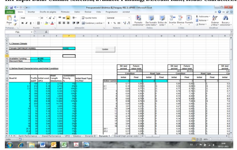
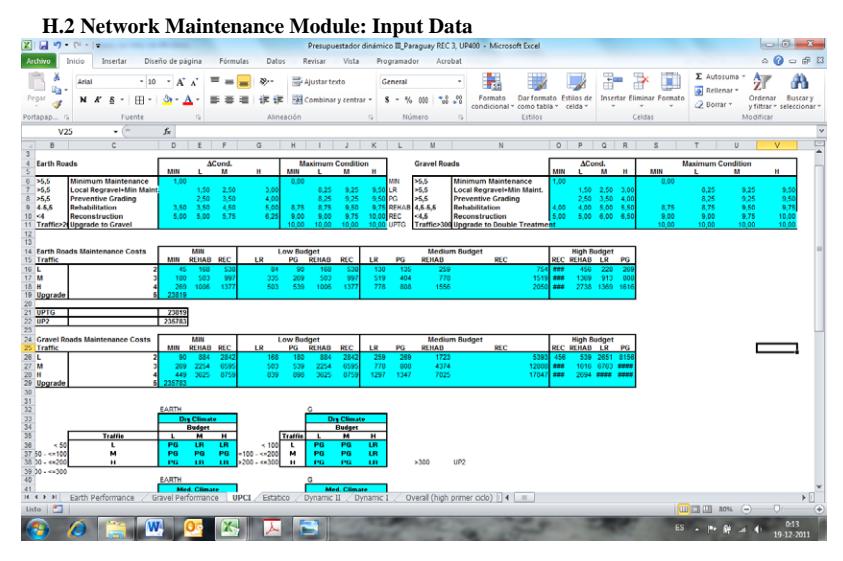
## **H.3 Network Analysis Interface: Condition and Cost Analysis per Cycle**
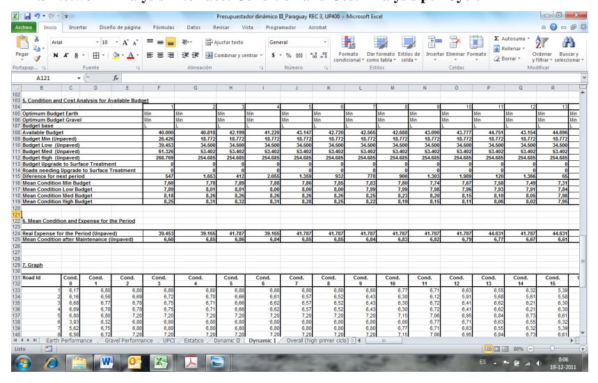
#### **Ap pplication n and Vali Append idation of dix I f the Man agement System**
#### **I.1 C hile Case S Study**
#### **I.1.1 1 Gravel Roa ads Conditio n per Road d: Chile Case Study**
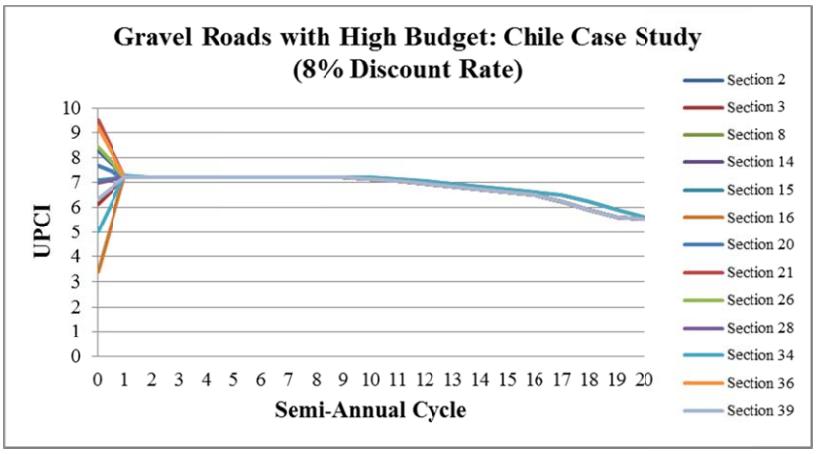
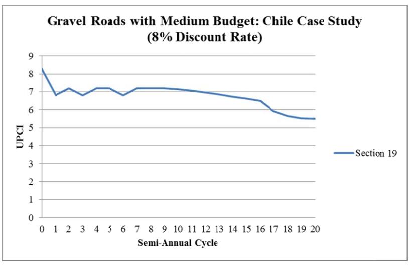
#### **I.1.2 Earth Roads Condition per Road: Chi le Case Study**
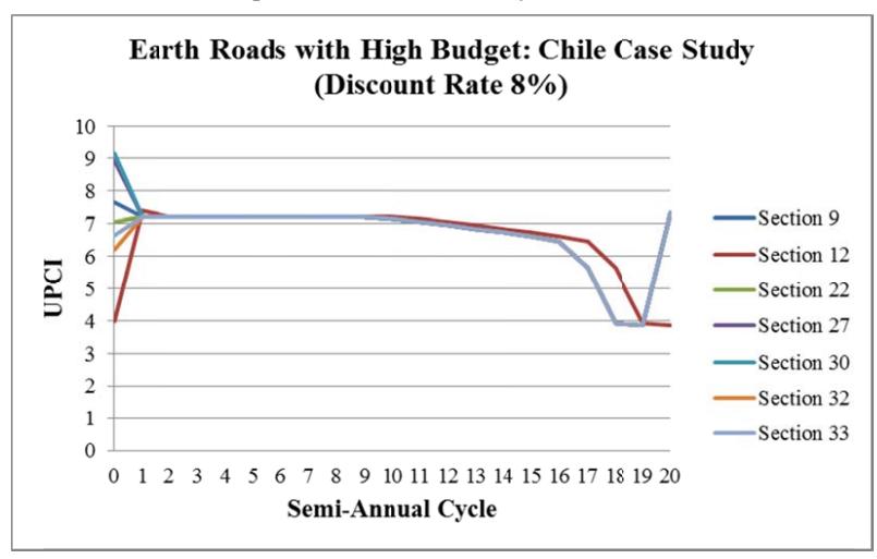
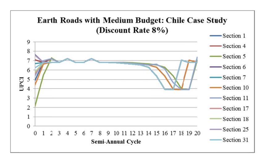
## **I.1.3 Condition Data Life Cycle Analysis: Chile Case Study**
| Ro
ad
Id | Ini
tial
Ro
ad
Ty
pe | Fin
al
Ro
ad
Ty
pe | ior
ity
Pr
Ra
nk | Cy
cle
0 | Cy
cle
1 | Cy
cle
2 | Cy
cle
3 | Cy
cle
4 | Cy
cle
5 | Cy
cle
6 | Cy
cle
7 | Cy
cle
8 | Cy
cle
9 | Cy
cle
10 | Cy
cle
11 | Cy
cle
12 | Cy
cle
13 | Cy
cle
14 | Cy
cle
15 | Cy
cle
16 | Cy
cle
17 | Cy
cle
18 | Cy
cle
19 | Cy
cle
20 |
|----------------|-------------------------------------|-----------------------------------|------------------------------|----------------|----------------|----------------|----------------|----------------|----------------|----------------|----------------|----------------|----------------|-----------------|-----------------|-----------------|-----------------|-----------------|-----------------|-----------------|-----------------|-----------------|-----------------|-----------------|
| 1 | E | E | 33 | 4.9 | 6.9 | 6.8 | 6.8 | 7.2 | 6.8 | 6.8 | 7.2 | 6.8 | 6.8 | 6.8 | 6.8 | 6.7 | 6.6 | 6.6 | 6.3 | 5.4 | 3.9 | 3.9 | 7.1 | 6.8 |
| 2 | G | G | 5 | 8.3 | 7.2 | 7.2 | 7.2 | 7.2 | 7.2 | 7.2 | 7.2 | 7.2 | 7.2 | 7.2 | 7.1 | 7.0 | 6.8 | 6.7 | 6.6 | 6.5 | 6.2 | 5.9 | 5.6 | 5.5 |
| 3 | G | G | 19 | 6.1 | 7.2 | 7.2 | 7.2 | 7.2 | 7.2 | 7.2 | 7.2 | 7.2 | 7.2 | 7.2 | 7.1 | 7.0 | 6.8 | 6.7 | 6.6 | 6.5 | 6.2 | 5.9 | 5.6 | 5.5 |
| 4 | E | E | 24 | 7.1 | 6.8 | 7.2 | 6.8 | 7.2 | 6.8 | 6.8 | 7.2 | 6.8 | 6.8 | 6.8 | 6.7 | 6.6 | 6.6 | 6.3 | 5.4 | 3.9 | 3.9 | 7.1 | 6.8 | 6.8 |
| 5 | E | E | 23 | 2.1 | 5.5 | 7.3 | 6.8 | 7.2 | 6.8 | 6.8 | 7.2 | 6.8 | 6.8 | 6.8 | 6.8 | 6.8 | 6.7 | 6.6 | 6.6 | 6.3 | 5.4 | 4.0 | 3.9 | 7.1 |
| 6 | E | E | 30 | 7.6 | 6.8 | 6.8 | 6.8 | 7.2 | 6.8 | 6.8 | 7.2 | 6.8 | 6.8 | 6.8 | 6.7 | 6.6 | 6.6 | 6.3 | 5.4 | 3.9 | 3.9 | 7.1 | 6.8 | 6.8 |
| 7 | E | E | 27 | 6.7 | 6.8 | 6.8 | 6.8 | 7.2 | 6.8 | 6.8 | 7.2 | 6.8 | 6.8 | 6.8 | 6.7 | 6.6 | 6.6 | 6.3 | 5.4 | 3.9 | 3.9 | 7.1 | 6.8 | 6.8 |
| 8 | G | G | 3 | 9.5 | 7.2 | 7.2 | 7.2 | 7.2 | 7.2 | 7.2 | 7.2 | 7.2 | 7.2 | 7.2 | 7.1 | 7.0 | 6.8 | 6.7 | 6.6 | 6.5 | 6.2 | 5.9 | 5.6 | 5.5 |
| 9 | E | E | 18 | 7.7 | 7.2 | 7.2 | 7.2 | 7.2 | 7.2 | 7.2 | 7.2 | 7.2 | 7.2 | 7.2 | 7.1 | 7.0 | 6.8 | 6.7 | 6.6 | 6.5 | 5.6 | 3.9 | 3.9 | 7.3 |
| 10 | E | E | 32 | 4.4 | 6.7 | 6.8 | 6.8 | 7.2 | 6.8 | 6.8 | 7.2 | 6.8 | 6.8 | 6.8 | 6.8 | 6.7 | 6.6 | 6.6 | 6.3 | 5.4 | 3.9 | 3.9 | 7.1 | 6.8 |
| 11 | E | E | 22 | 5.4 | 7.0 | 7.2 | 6.8 | 7.2 | 6.8 | 6.8 | 7.2 | 6.8 | 6.8 | 6.8 | 6.8 | 6.7 | 6.6 | 6.6 | 6.6 | 6.1 | 4.6 | 3.9 | 3.9 | 7.4 |
| 12 | E | E | 20 | 4.0 | 7.4 | 7.2 | 7.2 | 7.2 | 7.2 | 7.2 | 7.2 | 7.2 | 7.2 | 7.2 | 7.2 | 7.1 | 7.0 | 6.8 | 6.7 | 6.6 | 6.5 | 5.6 | 3.9 | 3.9 |
| 14 | G | G | 15 | 7.7 | 7.2 | 7.2 | 7.2 | 7.2 | 7.2 | 7.2 | 7.2 | 7.2 | 7.2 | 7.2 | 7.1 | 7.0 | 6.8 | 6.7 | 6.6 | 6.5 | 6.2 | 5.9 | 5.6 | 5.5 |
| 15 | G | G | 2 | 7.1 | 7.2 | 7.2 | 7.2 | 7.2 | 7.2 | 7.2 | 7.2 | 7.2 | 7.2 | 7.2 | 7.1 | 7.0 | 6.8 | 6.7 | 6.6 | 6.5 | 6.2 | 5.9 | 5.6 | 5.5 |
| 16 | G | G | 17 | 3.4 | 7.3 | 7.2 | 7.2 | 7.2 | 7.2 | 7.2 | 7.2 | 7.2 | 7.2 | 7.2 | 7.2 | 7.1 | 7.0 | 6.8 | 6.7 | 6.6 | 6.5 | 6.2 | 5.9 | 5.6 |
| 17 | E | E | 28 | 5.6 | 6.8 | 6.8 | 6.8 | 7.2 | 6.8 | 6.8 | 7.2 | 6.8 | 6.8 | 6.8 | 6.7 | 6.6 | 6.6 | 6.3 | 5.4 | 3.9 | 3.9 | 7.1 | 6.8 | 6.8 |
| 18 | E | E | 26 | 5.8 | 6.8 | 6.8 | 6.8 | 7.2 | 6.8 | 6.8 | 7.2 | 6.8 | 6.8 | 6.8 | 6.7 | 6.6 | 6.6 | 6.3 | 5.4 | 3.9 | 3.9 | 7.1 | 6.8 | 6.8 |
| 19 | G | G | 21 | 8.3 | 6.8 | 7.2 | 6.8 | 7.2 | 7.2 | 6.8 | 7.2 | 7.2 | 7.2 | 7.2 | 7.1 | 7.0 | 6.8 | 6.7 | 6.6 | 6.5 | 5.9 | 5.7 | 5.5 | 5.5 |
| 20 | G | G | 12 | 7.7 | 7.2 | 7.2 | 7.2 | 7.2 | 7.2 | 7.2 | 7.2 | 7.2 | 7.2 | 7.2 | 7.1 | 7.0 | 6.8 | 6.7 | 6.6 | 6.5 | 6.2 | 5.9 | 5.6 | 5.5 |
| 21 | G | G | 4 | 9.5 | 7.2 | 7.2 | 7.2 | 7.2 | 7.2 | 7.2 | 7.2 | 7.2 | 7.2 | 7.2 | 7.1 | 7.0 | 6.8 | 6.7 | 6.6 | 6.5 | 6.2 | 5.9 | 5.6 | 5.5 |
| 22 | E | E | 8 | 7.1 | 7.2 | 7.2 | 7.2 | 7.2 | 7.2 | 7.2 | 7.2 | 7.2 | 7.2 | 7.2 | 7.1 | 7.0 | 6.8 | 6.7 | 6.6 | 6.5 | 5.6 | 3.9 | 3.9 | 7.3 |
| 25 | E | E | 29 | 7.6 | 6.8 | 6.8 | 6.8 | 7.2 | 6.8 | 6.8 | 7.2 | 6.8 | 6.8 | 6.8 | 6.7 | 6.6 | 6.6 | 6.3 | 5.4 | 3.9 | 3.9 | 7.1 | 6.8 | 6.8 |
| 26 | G | G | 10 | 8.4 | 7.2 | 7.2 | 7.2 | 7.2 | 7.2 | 7.2 | 7.2 | 7.2 | 7.2 | 7.2 | 7.1 | 7.0 | 6.8 | 6.7 | 6.6 | 6.5 | 6.2 | 5.9 | 5.6 | 5.5 |
| 27 | E | E | 16 | 8.9 | 7.2 | 7.2 | 7.2 | 7.2 | 7.2 | 7.2 | 7.2 | 7.2 | 7.2 | 7.2 | 7.1 | 7.0 | 6.8 | 6.7 | 6.6 | 6.5 | 5.6 | 3.9 | 3.9 | 7.3 |
| 28 | G | G | 6 | 7.0 | 7.2 | 7.2 | 7.2 | 7.2 | 7.2 | 7.2 | 7.2 | 7.2 | 7.2 | 7.2 | 7.1 | 7.0 | 6.8 | 6.7 | 6.6 | 6.5 | 6.2 | 5.9 | 5.6 | 5.5 |
| 30 | E | E | 13 | 9.2 | 7.2 | 7.2 | 7.2 | 7.2 | 7.2 | 7.2 | 7.2 | 7.2 | 7.2 | 7.2 | 7.1 | 7.0 | 6.8 | 6.7 | 6.6 | 6.5 | 5.6 | 3.9 | 3.9 | 7.3 |
| 31 | E | E | 25 | 6.3 | 6.8 | 6.8 | 6.8 | 7.2 | 6.8 | 6.8 | 7.2 | 6.8 | 6.8 | 6.8 | 6.7 | 6.6 | 6.6 | 6.3 | 5.4 | 3.9 | 3.9 | 7.1 | 6.8 | 6.8 |
| 32 | E | E | 9 | 6.2 | 7.2 | 7.2 | 7.2 | 7.2 | 7.2 | 7.2 | 7.2 | 7.2 | 7.2 | 7.2 | 7.1 | 7.0 | 6.8 | 6.7 | 6.6 | 6.5 | 5.6 | 3.9 | 3.9 | 7.3 |
| 33 | E | E | 14 | 6.7 | 7.2 | 7.2 | 7.2 | 7.2 | 7.2 | 7.2 | 7.2 | 7.2 | 7.2 | 7.2 | 7.1 | 7.0 | 6.8 | 6.7 | 6.6 | 6.5 | 5.6 | 3.9 | 3.9 | 7.3 |
| 34 | G | G | 7 | 5.0 | 7.3 | 7.2 | 7.2 | 7.2 | 7.2 | 7.2 | 7.2 | 7.2 | 7.2 | 7.2 | 7.2 | 7.1 | 7.0 | 6.8 | 6.7 | 6.6 | 6.5 | 6.2 | 5.9 | 5.6 |
| 36 | G | G | 11 | 9.2 | 7.2 | 7.2 | 7.2 | 7.2 | 7.2 | 7.2 | 7.2 | 7.2 | 7.2 | 7.2 | 7.1 | 7.0 | 6.8 | 6.7 | 6.6 | 6.5 | 6.2 | 5.9 | 5.6 | 5.5 |
| 37 | G | PAV | 37 | 6.2 | 10 | 10 | 10 | 10 | 10 | 10 | 10 | 10 | 10 | 10 | 10 | 10 | 10 | 10 | 10 | 10 | 10 | 10 | 10 | 10 |
| 38 | G | PAV | 36 | 5.9 | 10 | 10 | 10 | 10 | 10 | 10 | 10 | 10 | 10 | 10 | 10 | 10 | 10 | 10 | 10 | 10 | 10 | 10 | 10 | 10 |
| 39 | G | G | 1 | 6.3 | 7.2 | 7.2 | 7.2 | 7.2 | 7.2 | 7.2 | 7.2 | 7.2 | 7.2 | 7.2 | 7.1 | 7.0 | 6.8 | 6.7 | 6.6 | 6.5 | 6.2 | 5.9 | 5.6 | 5.5 |
## **I.1.4 Sustainable Network Prioritization: Chile Case Study**
| Road | Priority | | Initial | | | Initial |
|------|----------|------|---------|------------|-------|-----------|
| Id | Rank | AADT | UPCI | Kilometres | % | Road Type |
| 1 | 33 | 4 | 4.9 | 0.55 | 0.1% | E |
| 2 | 5 | 100 | 8.3 | 13.9 | 3.3% | G |
| 3 | 19 | 30 | 6.1 | 2 | 0.7% | G |
| 4 | 24 | 6 | 7.1 | 2.8 | 0.4% | E |
| 5 | 23 | 14 | 2.1 | 1.4 | 0.5% | E |
| 6 | 30 | 10 | 7.6 | 0.4 | 0.3% | E |
| 7 | 27 | 10 | 6.7 | 0.5 | 0.5% | E |
| 8 | 3 | 70 | 9.5 | 9.7 | 8.7% | G |
| 9 | 18 | 14 | 7.7 | 2 | 1.2% | E |
| 10 | 32 | 8 | 4.4 | 0.85 | 0.2% | E |
| 11 | 22 | 12 | 5.4 | 5 | 0.3% | E |
| 12 | 20 | 30 | 4.0 | 1.5 | 0.6% | E |
| 14 | 15 | 50 | 7.7 | 4 | 1.2% | G |
| 15 | 2 | 100 | 7.1 | 7.7 | 10.0% | G |
| 16 | 17 | 30 | 3.4 | 3.3 | 0.6% | G |
| 17 | 28 | 6 | 5.6 | 1.1 | 0.3% | E |
| 18 | 26 | 6 | 5.8 | 1.7 | 0.2% | E |
| 19 | 21 | 20 | 8.3 | 3.2 | 0.6% | G |
| 20 | 12 | 40 | 7.7 | 5.8 | 1.2% | G |
| 21 | 4 | 80 | 9.5 | 11.7 | 5.0% | G |
| 22 | 8 | 40 | 7.1 | 6.8 | 1.6% | E |
| 25 | 29 | 16 | 7.6 | 1.2 | 0.1% | E |
| 26 | 10 | 60 | 8.4 | 11.2 | 1.9% | G |
| 27 | 16 | 20 | 8.9 | 3 | 0.8% | E |
| 28 | 6 | 80 | 7.0 | 5.3 | 6.2% | G |
| 30 | 13 | 30 | 9.2 | 3 | 1.9% | E |
| 31 | 25 | 6 | 6.3 | 2 | 0.3% | E |
| 32 | 9 | 60 | 6.2 | 5.4 | 3.1% | E |
| 33 | 14 | 30 | 6.7 | 1.6 | 1.2% | E |
| 34 | 7 | 60 | 5.0 | 10.2 | 4.0% | G |
| 36 | 11 | 40 | 9.2 | 4.9 | 1.5% | G |
| 37 | 37 | 220 | 6.2 | 15.9 | 15.5% | G |
| 38 | 36 | 260 | 5.9 | 15.9 | 15.5% | G |
| 39 | 1 | 100 | 6.3 | 11 | 10.5% | G |
#### **I.2 P araguay Ca se Study**
#### **I.2.1 Gravel Roa ds Condition per Road : Paraguay Case Study**
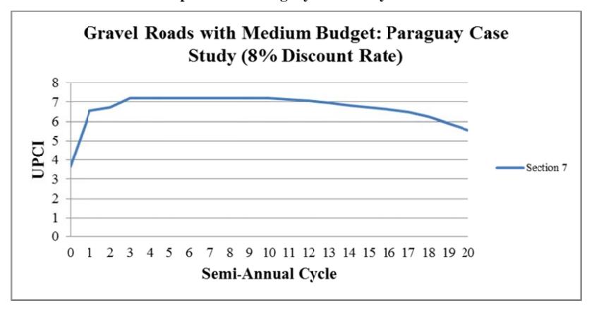
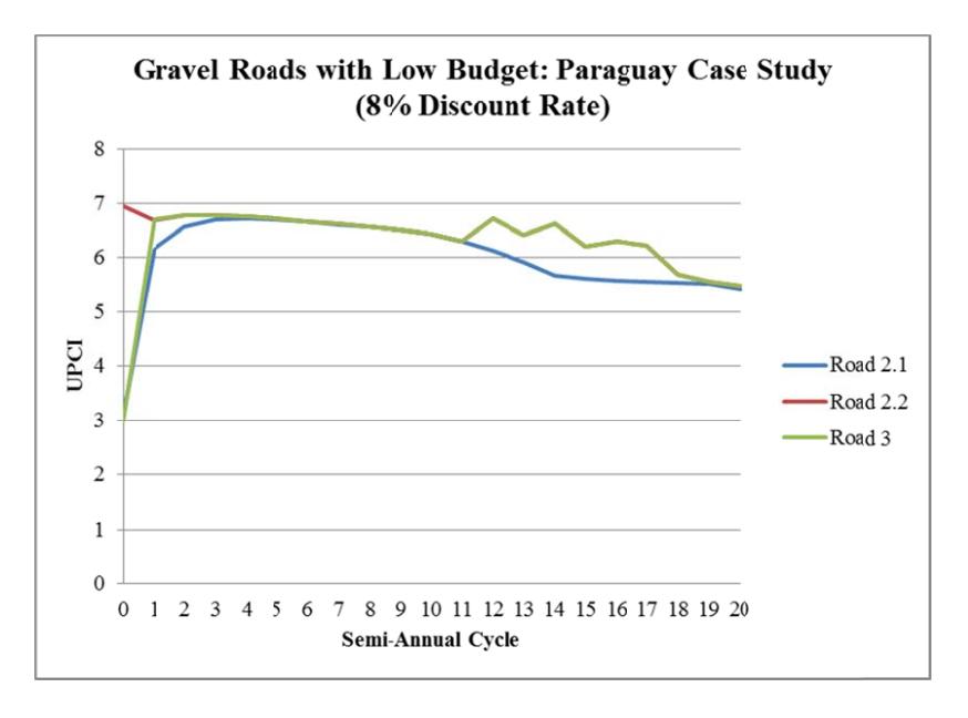
#### **I.2.2 Earth Roads Condition per Road: Par aguay Case Study**

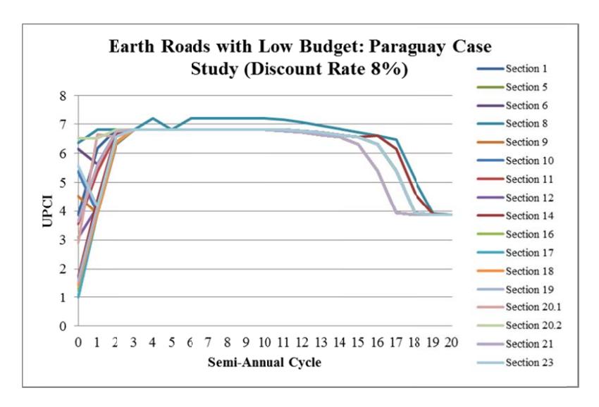
### **I.2.3 Condition Data Life Cycle Analysis: Paraguay Case Study**
| Ro
ad | Init
ial
Ro
ad | Fin
al
Ro
ad | Pri
orit
y | | | | | | | | | | | | | | | | | | | | | | |
|----------|-------------------------|-----------------------|------------------|-----------|-----------|-----------|-----------|-----------|-----------|-----------|-----------|-----------|-----------|-----------|----------|------------|------------|------------|------------|------------|------------|------------|------------|------------|------------|
| Id | Typ
e | Typ
e | Ran
k | Co
nd. | Co
nd. | Co
nd. | Co
nd. | Co
nd. | Co
nd. | Co
nd. | Co
nd. | Co
nd. | Co
nd. | Co
nd. | C
ond | . C
ond | . C
ond | . C
ond | . C
ond | . C
ond | . C
ond | . C
ond | . C
ond | . C
ond | . C
ond |
| | E/G
/PA
V | E/G
/PA
V | | 0 | 1 | 2 | 3 | 4 | 5 | 6 | 7 | 8 | 9 | 10 | 11 | 12 | 13 | 14 | 15 | 16 | 17 | 18 | 19 | 20 | 21 |
| 1 | E | E | 20 | 3.8
7 | 6.1
7 | 6.8
0 | 6.8
0 | 6.8
0 | 6.8
0 | 6.8
0 | 6.8
0 | 6.8
0 | 6.8
0 | 6.8
0 | 6.7
7 | 6.7
1 | 6.6
3 | 6.5
5 | 6.3
2 | 5.3
9 | 3.9
3 | 3.8
8 | 3.8
7 | 3.8
7 | 3.8
7 |
| 2.1 | G | G | 12 | 3.0
9 | 6.1
6 | 6.5
6 | 6.6
9 | 6.7
2 | 6.7
0 | 6.6
6 | 6.6
1 | 6.5
7 | 6.5
2 | 6.4
3 | 6.3
0 | 6.1
2 | 5.9
1 | 5.6
8 | 5.6
1 | 5.5
8 | 5.5
6 | 5.5
4 | 5.5
2 | 5.4
3 | 5.1
9 |
| 2.2 | G | G | 6 | 6.9
5 | 6.6
8 | 6.7
7 | 6.7
8 | 6.7
5 | 6.7
1 | 6.6
6 | 6.6
2 | 6.5
7 | 6.5
2 | 6.4
3 | 6.3
0 | 6.7
2 | 6.4
1 | 6.6
2 | 6.2
1 | 6.3
0 | 6.2
3 | 5.6
9 | 5.5
5 | 5.4
7 | 5.2
9 |
| 3 | G | G | 5 | 2.9
8 | 6.6
9 | 6.7
8 | 6.7
8 | 6.7
5 | 6.7
1 | 6.6
6 | 6.6
2 | 6.5
7 | 6.5
2 | 6.4
3 | 6.3
0 | 6.7
2 | 6.4
1 | 6.6
2 | 6.2
1 | 6.3
0 | 6.2
3 | 5.6
9 | 5.5
5 | 5.4
7 | 5.2
9 |
| 4 | E | E | 3 | 7.3
5 | 6.8
0 | 6.8
0 | 7.2
0 | 7.2
0 | 7.2
0 | 7.2
0 | 7.2
0 | 7.2
0 | 7.2
0 | 7.2
0 | 7.1
5 | 7.0
6 | 6.9
5 | 6.8
4 | 6.7
3 | 6.6
1 | 6.4
6 | 5.1
3 | 3.9
1 | 3.8
6 | 3.8
6 |
| 5 | E | E | 16 | 1.0
0 | 3.9
3 | 6.3
2 | 6.8
0 | 6.8
0 | 6.8
0 | 6.8
0 | 6.8
0 | 6.8
0 | 6.8
0 | 6.8
0 | 6.8
0 | 6.7
7 | 6.7
1 | 6.6
3 | 6.5
5 | 6.3
2 | 5.3
9 | 3.9
3 | 3.8
8 | 3.8
7 | 3.8
7 |
| 6 | E | E | 9 | 6.1
6 | 5.6
2 | 6.7
5 | 6.8
0 | 6.8
0 | 6.8
0 | 6.8
0 | 6.8
0 | 6.8
0 | 6.8
0 | 6.8
0 | 6.7
7 | 6.7
1 | 6.6
3 | 6.5
5 | 6.3
2 | 5.3
9 | 3.9
3 | 3.8
8 | 3.8
7 | 3.8
7 | 3.8
7 |
| 7 | G | G | 1 | 3.6
4 | 6.5
6 | 6.7
2 | 7.2
0 | 7.2
0 | 7.2
0 | 7.2
0 | 7.2
0 | 7.2
0 | 7.2
0 | 7.2
0 | 7.1
5 | 7.0
6 | 6.9
5 | 6.8
4 | 6.7
3 | 6.6
1 | 6.4
9 | 6.2
4 | 5.8
9 | 5.5
7 | 5.4
7 |
| 8 | E | E | 4 | 6.3
6 | 6.8
0 | 6.8
0 | 6.8
0 | 7.2
0 | 6.8
0 | 7.2
0 | 7.2
0 | 7.2
0 | 7.2
0 | 7.2
0 | 7.1
5 | 7.0
6 | 6.9
5 | 6.8
4 | 6.7
3 | 6.6
1 | 6.4
6 | 5.1
3 | 3.9
1 | 3.8
6 | 3.8
6 |
| 9 | E | E | 18 | 4.5
4 | 3.9
1 | 6.2
7 | 6.8
0 | 6.8
0 | 6.8
0 | 6.8
0 | 6.8
0 | 6.8
0 | 6.8
0 | 6.8
0 | 6.8
0 | 6.7
7 | 6.7
1 | 6.6
3 | 6.5
5 | 6.3
2 | 5.3
9 | 3.9
3 | 3.8
8 | 3.8
7 | 3.8
7 |
| 10 | E | E | 14 | 5.3
7 | 3.9
4 | 6.3
5 | 6.8
0 | 6.8
0 | 6.8
0 | 6.8
0 | 6.8
0 | 6.8
0 | 6.8
0 | 6.8
0 | 6.8
0 | 6.7
7 | 6.7
1 | 6.6
3 | 6.5
5 | 6.3
2 | 5.3
9 | 3.9
3 | 3.8
8 | 3.8
7 | 3.8
7 |
| 11 | E | E | 15 | 3.5
6 | 5.3
8 | 6.6
5 | 6.8
0 | 6.8
0 | 6.8
0 | 6.8
0 | 6.8
0 | 6.8
0 | 6.8
0 | 6.8
0 | 6.7
7 | 6.7
1 | 6.6
3 | 6.5
5 | 6.3
2 | 5.3
9 | 3.9
3 | 3.8
8 | 3.8
7 | 3.8
7 | 3.8
7 |
| 12 | E | E | 10 | 3.0
8 | 4.1
5 | 6.5
6 | 6.8
0 | 6.8
0 | 6.8
0 | 6.8
0 | 6.8
0 | 6.8
0 | 6.8
0 | 6.8
0 | 6.8
0 | 6.7
7 | 6.7
1 | 6.6
3 | 6.5
5 | 6.3
2 | 5.3
9 | 3.9
3 | 3.8
8 | 3.8
7 | 3.8
7 |
| 14 | E | E | 7 | 1.6
8 | 4.3
9 | 6.6
6 | 6.8
0 | 6.8
0 | 6.8
0 | 6.8
0 | 6.8
0 | 6.8
0 | 6.8
0 | 6.8
0 | 6.8
0 | 6.7
7 | 6.7
1 | 6.6
3 | 6.5
5 | 6.6
1 | 6.1
5 | 4.6
4 | 3.9
0 | 3.8
7 | 3.8
7 |
| 16 | E | E | 8 | 1.2
5 | 3.9
4 | 6.3
4 | 6.8
0 | 6.8
0 | 6.8
0 | 6.8
0 | 6.8
0 | 6.8
0 | 6.8
0 | 6.8
0 | 6.8
0 | 6.7
7 | 6.7
1 | 6.6
3 | 6.5
5 | 6.3
2 | 5.3
9 | 3.9
3 | 3.8
8 | 3.8
7 | 3.8
7 |
| 17 | E | E | 21 | 1.0
0 | 3.9
3 | 6.3
2 | 6.8
0 | 6.8
0 | 6.8
0 | 6.8
0 | 6.8
0 | 6.8
0 | 6.8
0 | 6.8
0 | 6.8
0 | 6.7
7 | 6.7
1 | 6.6
3 | 6.5
5 | 6.3
2 | 5.3
9 | 3.9
3 | 3.8
8 | 3.8
7 | 3.8
7 |
| 18 | E | E | 13 | 1.4
3 | 3.9
4 | 6.3
6 | 6.8
0 | 6.8
0 | 6.8
0 | 6.8
0 | 6.8
0 | 6.8
0 | 6.8
0 | 6.8
0 | 6.8
0 | 6.7
7 | 6.7
1 | 6.6
3 | 6.5
5 | 6.3
2 | 5.3
9 | 3.9
3 | 3.8
8 | 3.8
7 | 3.8
7 |
| 19 | E | E | 23 | 1.5
8 | 4.1
5 | 6.5
6 | 6.8
0 | 6.8
0 | 6.8
0 | 6.8
0 | 6.8
0 | 6.8
0 | 6.8
0 | 6.8
0 | 6.8
0 | 6.7
7 | 6.7
1 | 6.6
3 | 6.5
5 | 6.3
2 | 5.3
9 | 3.9
3 | 3.8
8 | 3.8
7 | 3.8
7 |
| 20.
1 | E | E | 23 | 2.9
0 | 6.6
6 | 6.5
6 | 6.8
0 | 6.8
0 | 6.8
0 | 6.8
0 | 6.8
0 | 6.8
0 | 6.8
0 | 6.8
0 | 6.7
7 | 6.7
1 | 6.6
3 | 6.5
5 | 6.3
2 | 5.3
9 | 3.9
3 | 3.8
8 | 3.8
7 | 3.8
7 | 3.8
7 |
| 20.
2 | E | E | 19 | 6.5
2 | 6.5
1 | 6.8
0 | 6.8
0 | 6.8
0 | 6.8
0 | 6.8
0 | 6.8
0 | 6.8
0 | 6.8
0 | 6.8
0 | 6.7
7 | 6.7
1 | 6.6
3 | 6.5
5 | 6.3
2 | 5.3
9 | 3.9
3 | 3.8
8 | 3.8
7 | 3.8
7 | 3.8
7 |
| 21 | E | E | 11 | 3.6
5 | 5.6
1 | 6.7
4 | 6.8
0 | 6.8
0 | 6.8
0 | 6.8
0 | 6.8
0 | 6.8
0 | 6.8
0 | 6.8
0 | 6.7
7 | 6.7
1 | 6.6
3 | 6.5
5 | 6.3
2 | 5.3
9 | 3.9
3 | 3.8
8 | 3.8
7 | 3.8
7 | 3.8
7 |
| 22 | E | E | 2 | 4.2
7 | 6.6
1 | 6.8
0 | 7.2
0 | 7.2
0 | 7.2
0 | 7.2
0 | 7.2
0 | 7.2
0 | 7.2
0 | 7.2
0 | 7.1
5 | 7.0
6 | 6.9
5 | 6.8
4 | 6.7
3 | 6.6
1 | 6.4
6 | 5.6
4 | 3.9
3 | 3.8
6 | 3.8
6 |
| 23 | E | E | 17 | 5.5
8 | 4.1
6 | 6.5
6 | 6.8
0 | 6.8
0 | 6.8
0 | 6.8
0 | 6.8
0 | 6.8
0 | 6.8
0 | 6.8
0 | 6.8
0 | 6.7
7 | 6.7
1 | 6.6
3 | 6.5
5 | 6.3
2 | 5.3
9 | 3.9
3 | 3.8
8 | 3.8
7 | 3.8
7 |
| | | | | | | | | | | | | | | | | | | | | | | | | | |
### **I.2.4 Sustainable Network Prioritization: Paraguay Case Study**
| Road Id | Priority
Rank | AADT | Initial
UPCI | Kilometres | % | Initial Road
Type |
|---------|------------------|------|-----------------|------------|-----|----------------------|
| 1 | 20 | 100 | 3,87 | 2,70 | 1% | E |
| 2.1 | 12 | 212 | 3,086 | 2,73 | 8% | G |
| 2.2 | 6 | 212 | 6,95 | 5,47 | 15% | G |
| 3 | 5 | 150 | 2,983 | 6,30 | 11% | G |
| 4 | 3 | 286 | 7,345 | 8,60 | 10% | E |
| 5 | 16 | 100 | 1 | 4,60 | 2% | E |
| 6 | 9 | 150 | 6,155 | 11,26 | 3% | E |
| 7 | 1 | 252 | 3,64 | 14,60 | 14% | G |
| 8 | 4 | 250 | 6,355 | 14,70 | 4% | E |
| 9 | 18 | 150 | 4,54 | 3,80 | 1% | E |
| 10 | 14 | 75 | 5,365 | 6,10 | 1% | E |
| 11 | 15 | 50 | 3,56 | 6,10 | 1% | E |
| 12 | 10 | 90 | 3,08 | 6,50 | 2% | E |
| 14 | 7 | 50 | 1,675 | 8,20 | 6% | E |
| 16 | 8 | 50 | 1,25 | 6,30 | 6% | E |
| 17 | 21 | 30 | 1 | 2,60 | 1% | E |
| 18 | 13 | 50 | 1,43 | 5,30 | 2% | E |
| 19 | 23 | 40 | 1,58 | 0,80 | 1% | E |
| 20.1 | 23 | 20 | 2,9 | 3,60 | 0% | E |
| 20.2 | 19 | 50 | 6,52 | 3,60 | 1% | E |
| 21 | 11 | 70 | 3,65 | 3,70 | 4% | E |
| 22 | 2 | 83 | 4,265 | 11,00 | 8% | E |
| 23 | 17 | 60 | 5,5815625 | 3,10 | 1% | E |
#### **Sensitiv ity Analy Append ysis of the ix J Management System**
#### **I.1 Sensitivity A nalysis: Clim ate**
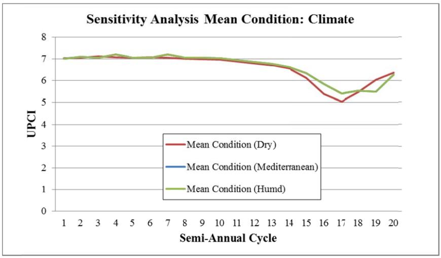
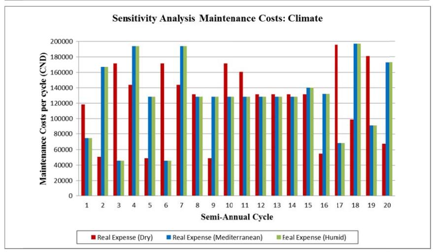
## **I.2 Sensitivity Analysis: Budget**

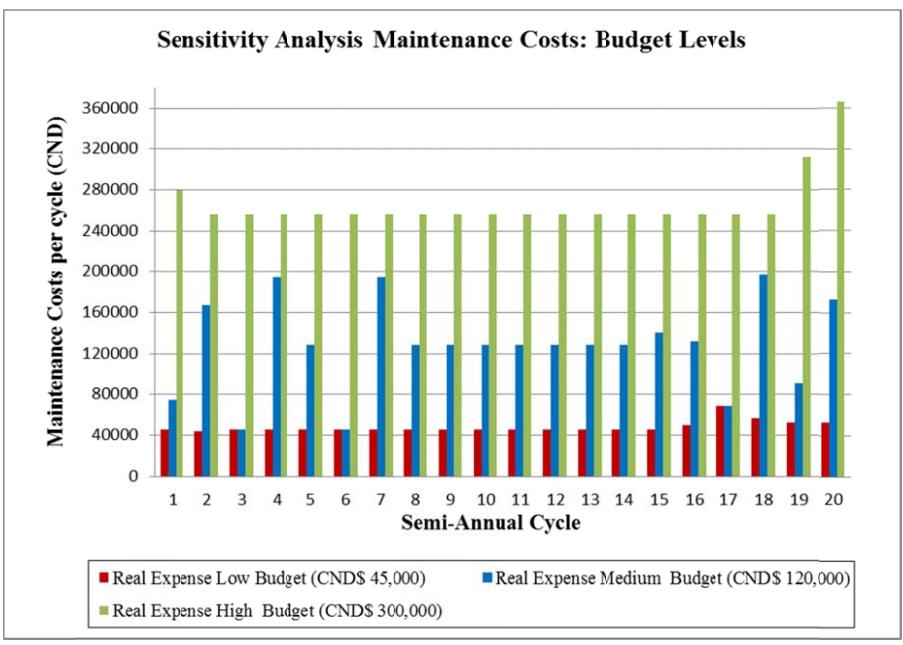
### **I.3 Sensitivity Analysis: Discount Rate**