---
category: literaturenote
citekey: zhaoalternativesestimatingseasonalfactors2008
title: "Alternatives for Estimating Seasonal Factors on Rural and Urban Roads in Florida, Phase II"
authors: "Zhao, Fang; Yang, Shanshan; Lu, Chenxi"
year: 2008
date: 2008-02-00 2008/02/00
url: "https://trid.trb.org/view.aspx?id=859631"
zotero_key: 8CV8VR3Z
zotero_storage: NPI6CQSP
collections: magistritöö / kohalikud teed
folder: 001_artiklid
firstAuthor: "Zhao, Fang"
status: converted
---
# **ALTERNATIVES FOR ESTIMATING SEASONAL FACTORS ON RURAL AND URBAN ROADS IN FLORIDA (PHASE II)**
**Final Report Contract No. BD015-17**
**Prepared for**
**Research Office Florida Department of Transportation**
**Lehman Center for Transportation Research Department of Civil & Environmental Engineering Florida International University**
**February 2008**
# **ALTERNATIVES FOR ESTIMATING SEASONAL FACTORS ON RURAL AND URBAN ROADS IN FLORIDA, PHASE II**
Contract No. BD-015-17
### **Final Report**
Prepared for Florida Department of Transportation
Submitted by
Fang Zhao, Ph.D., P.E. Professor and Deputy Director
> Shanshan Yang, M.S. Research Assistant
> > and
Chenxi Lu, Ph.D. Research Assistant
Lehman Center for Transportation Research Department of Civil & Environmental Engineering Florida International University University Park Campus, EAS 3673 Miami, Florida 33199 Phone: 305-348-3821
Fax: 305-348-2802 E-mail: zhaof@fiu.edu
### **DISCLAIMER**
The contents of this report reflect the views of the authors and do not necessarily reflect the official views or policies of the Florida Department of Transportation. This report does not constitute a standard, specification, or regulation.
| 1. Report No.
Final Report for BD-015-17 | 2. Government Accession No. | 3. Recipient's Catalog No. | | |
|-----------------------------------------------------------------------------------------------------------------------------------------------------------------------------------------------------------|------------------------------------------------------------------------------------------------------------------|---------------------------------------|--|--|
| 4. Title and Subtitle
ALTERNATIVES FOR ESTIMATING SEASONAL FACTORS
ON RURAL AND URBAN ROADS IN FLORIDA, PHASE II | 5. Report Date
February 2008
6. Performing Organization Code | | | |
| 7. Author(s)
Fang Zhao, Shanshan Yang, Chenxi Lu | | 8. Performing Organization Report No. | | |
| 9. Performing Organization Name and Address
Lehman Center for Transportation Research, Department of Civil
and Environmental Engineering, Florida International University,
Miami, Florida 33199 | 10. Work Unit No. (TRAIS)
11. Contract or Grant No.
BD-015-17 | | | |
| 12. Sponsoring Agency Name and Address
Research Office
Florida Department of Transportation
650 Suwannee Street, MS 30
Tallahassee, Florida 32399-0450 | 13. Type of Report and Period Covered
Final Report
July 2006 – February 2008
14. Sponsoring Agency Code | | | |
#### 15. Supplementary Notes
#### 16. Abstract
Current practice at the Florida Department of Transportation (FDOT) employs seasonal factors (SFs) in the calculation of annual average daily traffic (AADT) at portable traffic monitoring sites (PTMS). Permanent traffic monitoring sites (TTMSs) are first manually classified into different groups (known as seasonal categories). These groups are based on similarities in the traffic characteristics of roads and on engineering judgment. FDOT districts then assign a seasonal factor category to each PTMS according to the site's functional classification and geographical location. It is assumed that seasonal variability and traffic characteristics at the short-term and permanent count sites are similar in the same geographic area. A previous study investigated traffic and land use data in Southeast and North Florida, with the goal of making the seasonal factor assignment process more objective and data-driven, as this would improve the accuracy in AADT estimation for PTMSs. The results from that study demonstrated the possibility of identifying the link between land use variables and seasonal factors. In this follow-up study, a state-wide investigation is conducted, and multiple linear regression analyses are carried out. These are used to identify possible factors contributing to the seasonal fluctuations in traffic volumes for urban and rural locations with a TTMS in Florida. Based on these factors, a methodology is developed to determine which TTMSs are most likely to share similar seasonal factors with a PTMS in urban areas. This methodology may be improved and expanded for application to rural areas.
| 17. Key Word
Seasonal Factors, AADT, Cluster Analysis, Traffic
Monitoring, Regression Analysis, Seasonal Factor
Assignment | | 18. Distribution Statement | | |
|-------------------------------------------------------------------------------------------------------------------------------------|--|----------------------------|-------------------------|-----------|
| 19. Security Classif. (of this report)
20. Security Classif. (of this page)
Unclassified.
Unclassified. | | | 21. No. of Pages
212 | 22. Price |
**Form DOT F 1700.7** (8-72) Reproduction of completed page authorized
### **ACKNOWLEDGEMENTS**
This research was funded by the Research Center of the Florida Department of Transportation. The supports from the FDOT are gratefully acknowledged. The authors would also like to thank the project managers, Mr. Richard Reel of the Traffic Data Section of FDOT Transportation Statistics Office and Mr. Doug O'Hara of FDOT District 4, for their support and guidance. Thanks also go to Dr. Lee-Fang Chow and Dr. Soon Chung, for their help with computer scripts used to compile the data used in this project. This report has been edited by Mr. Mark Mandell, Technical Editor of Lehman Center for Transportation Research.
### **EXECUTIVE SUMMARY**
This research is a follow-up study to a previous project. The project entailed an investigation of the problems with seasonal factor grouping and assigning TTMS groups to coverage count sites. The previous study involved limited urban areas in Southeast Florida and rural areas in North Florida. The present study expands the investigation to all of the urban and rural areas in Florida. The goal of this expansion is to provide the necessary knowledge to implement a practical tool that can be used for estimating seasonal factors for coverage counts statewide.
The research involved the following: imputation of TTMS data, clustering of TTMSs to create seasonal factor groups, conducting regression analysis to identify influential land use variables that may affect seasonal factors, and a preliminary study of possible assignment methods.
Imputation refers to the replacement of missing data with a substitute. This substitute allows data analysis to be conducted without being misleading. This is important because there are less than 300 TTMSs in service, and 24.2% of them are missing data from the year 2000. The imputation method adopted in this study is easily understood and implemented.
Cluster analysis has been applied to statewide TTMSs to create seasonal factor groups. A modelbased cluster technique using only the 12 MSFs proves to be more practical and produces reasonable results.
Regression models are developed to identify influential variables for the seasonal factors of TTMSs. It is found that influential variables for the seasonal factors of the TTMSs are different in urban and rural areas and in different climate zones. The state is divided into three climate zones. Separate models are developed for each zone. For North Florida, the most influential variables are as follows: whether a TTMS is close to a urban freeway; employment related to hotels and camps; employment related to museums, art galleries, and gardens; retired households; seasonal households; population ages 11-17; retired households with low income; residential university; etc. For Central Florida, important variables are agriculture workers; proximity of a TTMS to an urban collector, minor arterial, or principal arterial; median household income; retired households; seasonal households; population ages 11-17; low-income retired households; etc*.* For South Florida, hotels, museums, manufacturing employment, retired and seasonal households, and proximity to principal arterials are significant variables.
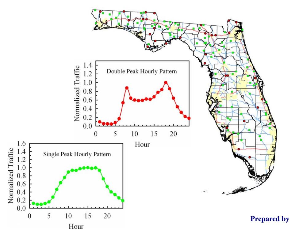
The approach for modeling the urban area TTMSs cannot be applied to rural TTMSs. This is because there is an insufficient number of TTMSs in which to divide the rural areas to model them separately. An alternative approach is developed to separately model those TTMSs for which the hourly traffic pattern on a typical weekday shows a single peak (i.e., recreational travel dominates) and those of which the weekday hourly traffic pattern has a double peak (i.e., commute travel dominates). Some variables are significant regardless of whether the TTMSs' hourly traffic patterns show a single or double peak. These include the distance to and population of a nearby urban area, seasonal households in South Florida, and retail employees in South Florida. For TTMSs with a single peak, manufacturing employment, a truck factor, and the population between ages 18 and 64 are also found to be important. Likewise, the distance from a TTMS to the closest public beach is found to be important for the double-peak TTMSs. Several variables describe the spatial proximity to nearby urban areas and the roadway function class. The significance of these variables suggests that the basis for some current practices, such as considering function class and roadway use, may be valid in rural areas.
For the purpose of assigning seasonal factors to a coverage count site, the influential variables obtained from the urban models are used in developing a method to identify a TTMS. This TTMS will be similar to a given count station in terms of land uses or roadway functions. A similarity score is developed to measure the similarity between two count sites. This score is based on the identified influential variables, which are weighted by their partial R2 values in the models. This approach shows promising results: The average of standard errors in estimated seasonal factors is about 5% overall.
To further develop the results from this study for implementation, the following research efforts are recommended:
- 1) Conduct a more detailed analysis of the results of the assignment method to evaluate its accuracy. This is accomplished by determining the distribution of the errors. Note that this distribution includes the ranges, in addition to the currently used aggregate measure of mean errors. Understanding the locations or the characteristics of TTMSs where large errors occur will help identify variables that may be inappropriate. It can also indicate the need for additional variables.
- 2) Apply the proposed method to the assignment of seasonal factors in rural areas. Depending on the results, there may be a need to improve the regression models by identifying additional variables or to improve the definitions of existing variables.
- 3) Investigate the effect of inclusion or exclusion of different variables. For instance, if the exclusion of a variable does not change the assignment results, this variable may be left out to simplify the problem. Conversely, if a variable improves assignment results, it may be included even if its partial R2 from regression analysis is somewhat low. The effectiveness of the weighting scheme and alternative weighting schemes may also be examined to improve the assignment results.
- 4) Explore the feasibility of estimating each of the monthly seasonal factors for a given PTMS based on the influential variables in the regression equation corresponding to the same month. This is done as opposed to matching a PTMS to a TTMS and borrowing all of the monthly seasonal factors from that TTMS.
- 5) Compare the assignment results from the proposed approach to those obtained using the existing method. Note that, in the existing method, the average of the seasonal factors of a TTMS group is assigned to a coverage count site.
- 6) Independently test the assignment methods by using data collected monthly from selected sites that are different from the existing TTMSs in terms of geographic location and land use and roadway characteristics. This testing serves two purposes. One is to validate the proposed assignment methods. The other is to investigate the distribution of existing
TTMSs to determine whether they provide adequate coverage by representing a wide range, commonly encountered combinations of land uses and roadway types. In the assignment process, redundant TTMSs may be identified if many in relative spatial proximity are found to be similar to nearby PTMSs in both their land use and roadway characteristics and in their seasonal factors. Conversely, an area may also be identified as needing additional TTMSs because of their unique land use and roadway functions. To remove redundant TTMSs will reduce the operating and maintenance costs. The saved resources may be reinvested by adding TTMSs to needed areas to improve the accuracy of AADT estimation.
### **TABLE OF CONTENTS**
| 6.4 | Assignment in Urban Areas within FDOT Districts and Based on a Reduced | |
|-----|------------------------------------------------------------------------|--|
| | Variable Set125 | |
| 6.5 | Evaluation of the Three Assignment Strategies133 | |
| | 7. CONCLUSIONS AND RECOMMENDATIONS
135 | |
| | REFERENCES138 | |
| | APPENDIX A. IMPUTATION OF MSFS FOR URBAN AREA139 | |
| | APPENDIX B. IMPUTATION OF MSFS FOR RURAL AREA
165 | |
| | APPENDIX C. EMPLOYMENT VARIABLES
193 | |
| | APPENDIX D. LIST OF MODEL VARIABLES
195 | |
| | | |
### **LIST OF TABLES**
| Table 2.1 | Sample Seasonal Factor Database on FTI CD | 6 |
|------------|-------------------------------------------------------------------------|-----|
| Table 2.2 | List of TTMSs with Missing Data in Urban Areas | 7 |
| Table 2.3 | List of TTMSs with Missing Data in Rural Areas | 8 |
| Table 2.4 | Imputation of Site 930099
| 10 |
| Table 2.5 | Imputation of Site 930174
| 11 |
| Table 2.6 | Imputation of Site 740047
| 12 |
| Table 2.7 | List of TTMS with Missing Data after Imputation | 13 |
| Table 3.2 | Comparison of MOE for Rural Area
| 17 |
| Table 3.3 | Comparison of Cluster Analyses for Urban TTMSs | 18 |
| Table 3.4 | Number of TTMS Stations in the Optimal Ten Urban Groups
| 18 |
| Table 3.5 | Number of TTMS Stations in the Optimal 33 Urban Groups from Model | |
| | Based Cluster Analysis with Location Variables | 21 |
| Table 3.6 | TTMSs in Urban Groups 1, 3, 7, 8, and 9 | 22 |
| Table 3.7 | Number of the TTMSs in the 20 Urban Groups
| 45 |
| Table 3.8 | Comparison of Cluster Analyses for Rural TTMSs | 45 |
| Table 3.9 | Number of TTMSs in the Optimal Nine Groups
| 46 |
| Table 3.10 | Number of TTMSs in the Optimal 44 Groups | 48 |
| Table 3.11 | Number of TTMSs in the 28 Rural Groups
| 77 |
| Table 4.1 | Roadway Characteristic Variables for Urban Roads
| 79 |
| Table 4.2 | Student Population Age Group Variables | 80 |
| Table 4.3 | Retired Household Variables Based on State-Wide Median Income
| 80 |
| Table 4.4 | Employment Variables for Urban Roads | 81 |
| Table 4.5 | Location Characteristic Variables for Urban Roads
| 81 |
| Table 4.6 | Land Use Dummy Variables for Urban Road | 83 |
| Table 4.7 | List of Counties within the North Florida Analysis Area | 86 |
| Table 4.8 | Study Areas in Central Florida
| 87 |
| Table 4.9 | List of Counties within the South Florida Analysis Area | 88 |
| Table 4.10 | Regression Models for North Florida (NFL) | 89 |
| Table 4.11 | Variables from Model NFL Sorted by Month and Partial R2
Value | 91 |
| Table 4.12 | Variables from Model NFL Sorted by Name and Partial R2
Value | 91 |
| Table 4.13 | Variables from Model NFL Sorted by Partial R2
Value | 92 |
| Table 4.14 | Regression Models for Central Florida (CFL) | 93 |
| Table 4.15 | Variables from Model CFL Sorted by Month and Partial R2
Value | 94 |
| Table 4.16 | Variables from Model CFL Sorted by Name and Partial R2
Value | 95 |
| Table 4.17 | Variables from Model CFL Sorted by Partial R2
Value
| 95 |
| Table 4.19 | Variables from Model SFL Sorted by Month and Partial R2
Value
| 97 |
| Table 4.20 | Variables from Model SFL Sorted by Name and Partial R2
Value
| 97 |
| Table 4.21 | Variables from Model SFL Sorted by Partial R2
Value | 97 |
| Table 5.1 | Roadway Characteristic Variables for Rural Roads
| 98 |
| Table 5.2 | Age Group Variables for Rural Roads | 99 |
| Table 5.3 | Special Location Variables
| 100 |
| Table 5.4 | Socioeconomic and Demographic Variables for Different Climate Zones
| 100 |
| Table 5.5 | Regression Models for the Single-Peak Group for Rural Areas | 106 |
| Table 5.6 | Model Variables for Rural SP Group Sorted by Month and Partial R2
Value | 107 |
|------------|----------------------------------------------------------------------------|-----|
| Table 5.7 | Model Variables for Rural SP Group Sorted by Name and Partial R2
Value | 107 |
| Table 5.8 | Model Variables for Rural SP Group Sorted by Partial R2
Value
| 108 |
| Table 5.9 | Regression Models for Rural DP Group | 110 |
| Table 5.10 | Model Variables for Rural DP Group Sorted by Month and Partial R2 | |
| | value | 111 |
| Table 5.11 | Model Variables for Rural DP Group Sorted by Name and Partial R2 | |
| | Value | 111 |
| Table 5.12 | Model Variables for Rural DP Group Sorted by Partial R2
Value
| 111 |
| Table 6.1 | Variable Sets Used for Assignment for Model Regions | 114 |
| Table 6.2 | Assignment Results for TTMSs in North Florida | 114 |
| Table 6.3 | Assignment Results for TTMSs in Central Florida
| 116 |
| Table 6.4 | Assignment Results for TTMSs in South Florida | 117 |
| Table 6.5 | Seasonal Factors for the Sample Site 899921 and the First Five Best | |
| | Matched Sites | 119 |
| Table 6.6 | Reduced Variable Sets Used for Assignment for Three Model Regions | 121 |
| Table 6.7 | Assignment for North Florida with Reduced Variables
| 121 |
| Table 6.8 | TTMSs Assignment for Central Florida with Reduced Parameters
| 122 |
| Table 6.9 | Assignment Results for South Florida with a Reduced Variable Set
| 123 |
| Table 6.10 | Variable Sets Used for Assignment for Seven FDOT Districts | 126 |
| Table 6.11 | Assignment Results for District 1 with a Reduced Variable Set
| 127 |
| Table 6.12 | Assignment Results for District 2 with a Reduced Variable Set
| 127 |
| Table 6.13 | Assignment Results for District 3 with a Reduced Variable Set
| 128 |
| Table 6.14 | Assignment Results for District 4 with a Reduced Variable Set
| 129 |
| Table 6.15 | Assignment Results for District 5 with a Reduced Variable Set
| 130 |
| Table 6.16 | Assignment Results for District 6 with a Reduced Variable Set
| 131 |
| Table 6.17 | Assignment Results for District 7 with a Reduced Variable Set
| 131 |
| Table 6.18 | MSFs for Test Site 899921 and the First Five Best Matching Sites in | |
| | District 4 | 132 |
| Table 6.19 | Average Errors of the Assignment Results Based on Full Variable Set | 133 |
| Table 6.20 | Average Errors of the Assignment Results Based on a Reduced Variable | |
| | Set
| 134 |
| Table 6.21 | Average Errors of the Assignment Results Based on a Reduced Variable | |
| | Set within a District
| 134 |
### **LIST OF FIGURES**
| | 9 |
|------------------------------------------------------------------------|-----------------------------------------------------------------------------------------------------------------------------------------------------------------------------------------------------------------------------------------------------------------------------------------------------------------------------------------------------------------------------------------------------------------------------------------------------------------------------------------------------------------------------------------------------------------------------------------------------------------------------------------------------------------------------------------------------------------------------------------------------------------------------------------------------------------------------------------------------------------------------------------------------------------------------------------------------------------------------------------------------------------------------------------------------------------------------------------------------------------------------------------------------------------------------------------------------------------------------------------------------|
| | 10 |
| | 11 |
| Urban and Rural Area Definition | 14 |
| Optimal Ten Groups from Model-Based Method for Urban Areas | 19 |
| Optimal 33 Groups for Urban Areas from the Model-Based Method with | |
| Location Variables Included | 20 |
| Spatial Distribution and Profiles of the TTMSs in Urban Group 1
| 23 |
| Spatial Distribution and Profiles of the TTMSs in Urban Group 3
| 24 |
| Spatial Distribution and Profiles of the TTMSs in Urban Group 7
| 25 |
| Spatial Distribution and Profiles of the TTMSs in Urban Group 8
| 26 |
| Spatial Distribution and Profile of the TTMS in Urban Group 9
| 27 |
| Spatial Distribution and Profiles of the TTMSs in Urban Group 2
| 28 |
| Spatial Distribution of the Three New Subgroups for the Urban Group 2 |
29 |
| Profiles of the TTMSs in the New Urban Group 21 | 29 |
| Profiles of the TTMSs in the New Urban Group 22 | 30 |
| Profiles of the TTMSs in the New Urban Group 23 | 30 |
| Spatial Distribution and Profiles of the TTMSs in the Original Urban | |
| Group 4
| 31 |
| Spatial Distribution of the Three New Subgroups for the Original Urban | |
| Group 4
| 32 |
| | 32 |
| | 33 |
| | 33 |
| | |
| | 34 |
| | |
| | 35 |
| | 35 |
| | 36 |
| | |
| | 37 |
| | |
| | 38 |
| | 39 |
| | 39 |
| | 40 |
| | 40 |
| | |
| | 41 |
| | |
| | 42 |
| | 42 |
| | 43 |
| | Historical Data Plot for Site 930099
Historical Data plot of Site 930174
Historical Data Plot for Site 740047
Profiles of the TTMSs in the New Urban Group 41
Profiles of the TTMSs in the New Urban Group 42
Profiles of the TTMSs in the New Urban Group 43
Spatial Distribution and Profiles of the TTMS in the Original Urban
Group 5
Spatial Distribution of the Two New Subgroups for the Original Urban
Group 5
Profiles of the TTMSs in the New Urban Group 51
Profiles of the TTMSs in the New Urban Group 52
Spatial Distribution and Profiles of the TTMS in the Original Group
Urban 6
Spatial Distribution of the Four New Subgroups for the Original Urban
Group 6
Profiles of the TTMSs in the New Urban Group 61
Profiles of the TTMSs in the New Urban Group 62
Profiles of the TTMSs in the New Urban Group 63
Profiles of the TTMSs in the New Urban Group 64
Spatial Distribution and Profiles of the TTMSs in the Original Urban
Group 10
Spatial Distribution of the Three New Subgroups for the Original Urban
Group 10
Profiles of the TTMSs in the New Urban Group 101
Profiles of the TTMSs in the New Urban Group 102 |
| Figure 3.33 | Profiles of the TTMSs in the New Urban Group 103 | 43 |
|-------------|----------------------------------------------------------------------|----|
| Figure 3.34 | Modified Spatial Distribution of the TTMSs in Urban Areas
| 44 |
| Figure 3.35 | Optimal Nine Groups from Model-Based Clustering for TTMSs in Rural | |
| | Areas
| 46 |
| Figure 3.36 | Optimal 44 Groups Based on Model-Based Clustering with X-Y for Rural | |
| | Areas
| 47 |
| Figure 3.37 | Spatial Distribution and Profiles of the TTMSs in Rural Group 2
| 49 |
| Figure 3.38 | Spatial Distribution and Profiles of the TTMSs in Rural Group 8
| 50 |
| Figure 3.39 | Spatial Distribution and Profiles of the TTMSs in Rural Group 9
| 51 |
| Figure 3.40 | Spatial Distribution and Profiles of the TTMSs in Rural Group 1
| 52 |
| Figure 3.41 | New Subgroups Based on Rural Group 1 | 53 |
| Figure 3.42 | Profiles of TTMSs in the New Rural Group 11 | 53 |
| Figure 3.43 | Profiles of TTMSs in the New Rural Group 12 | 54 |
| Figure 3.44 | Profiles of TTMSs in the New Rural Group 13 | 54 |
| Figure 3.45 | Profiles of TTMSs in the New Rural Group 14 | 55 |
| Figure 3.46 | Profiles of TTMSs in the New Rural Group 15 | 55 |
| Figure 3.47 | Profiles of TTMSs in the New Rural Group 16 | 56 |
| Figure 3.48 | Spatial Distribution and Profiles of TTMSs in Rural Group 3
| 57 |
| Figure 3.49 | Four New Subgroups Created Based on Rural Group 3 | 58 |
| Figure 3.50 | Profiles of TTMSs in the New Rural Group 31 | 58 |
| Figure 3.51 | Profiles of TTMSs in the New Rural Group 32 | 59 |
| Figure 3.52 | Profiles of TTMSs in the New Rural Group 33 | 59 |
| Figure 3.53 | Profiles of TTMSs in the New Rural Group 34 | 60 |
| Figure 3.54 | Spatial Distribution and Profiles of TTMSs in Rural Group 4
| 61 |
| Figure 3.55 | Four New Subgroups Created Based on Rural Group 4 | 62 |
| Figure 3.56 | Profiles of TTMSs in the New Rural Group 41 | 62 |
| Figure 3.57 | Profiles of TTMSs in the New Rural Group 42 | 63 |
| Figure 3.58 | Profiles of TTMSs in the New Rural Group 43 | 63 |
| Figure 3.59 | Profiles of TTMSs in the New Rural Group 44 | 64 |
| Figure 3.60 | Spatial Distribution and Profiles of TTMSs in Rural Group 5
| 66 |
| Figure 3.61 | Four New Subgroups Created from Rural Group 5 | 66 |
| Figure 3.62 | Profiles of TTMSs in the New Rural Group 51 | 67 |
| Figure 3.63 | Profiles of TTMSs in the New Rural Group 52 | 67 |
| Figure 3.64 | Profiles of TTMSs in the New Rural Group 53 | 68 |
| Figure 3.65 | Profiles of TTMSs in the New Rural Group 54 | 68 |
| Figure 3.66 | Spatial Distribution and Profile of TTMSs in Rural Group 6 | 69 |
| Figure 3.67 | Four New Subgroups Created from Rural Group 6 | 70 |
| Figure 3.68 | Profiles of TTMSs in the New Rural Group 61 | 71 |
| Figure 3.69 | Profiles of TTMSs in the New Rural Group 62 | 71 |
| Figure 3.70 | Profiles of TTMSs in the New Rural Group 63 | 71 |
| Figure 3.71 | Profiles of TTMSs in the New Rural Group 64 | 72 |
| Figure 3.72 | Spatial Distribution and Profiles of the TTMSs in Rural Group 7
| 73 |
| Figure 3.73 | Three New Subgroups Created from Rural Group 7
| 74 |
| Figure 3.74 | Profiles of TTMSs in the New Rural Group 71 | 74 |
| Figure 3.75 | Profiles of TTMSs in the New Rural Group 72 | 75 |
| Figure 3.76 | Profiles of TTMSs in the New Rural Group 73 | 75 |
| | | |
| Figure 3.77 | Spatial Distribution of Modified TTMS Groups in Rural Areas
| 76 |
|-------------|---------------------------------------------------------------------------|-----|
| Figure 4.1 | Water Management Districts in Florida (Source: Florida Department of | |
| | Environmental Protection) | 82 |
| Figure 4.2 | Land Use and TTMSs in Urban Areas | 83 |
| Figure 4.4 | TTMSs in Three Urban Study Areas in North Florida
| 86 |
| Figure 4.5 | TTMSs in Five Urban Study Areas in Central Florida | 87 |
| Figure 4.6 | TTMSs in Four Urban Study Areas in South Florida | 88 |
| Figure 5.1 | Single-Peak Pattern and Variables Describing Peaking Characteristics | 102 |
| Figure 5.2 | Double-Peak Pattern and Variables Describing Peaking Characteristics | 102 |
| Figure 5.3 | Hourly Traffic Variations for Selected TTMSs | 103 |
| Figure 5.4 | Hourly Traffic Pattern for TTMSs | 104 |
| Figure 6.1 | Seasonal Factors for the Test Site 899921 and the First Five Closest | |
| | Matching Sites
| 119 |
| Figure 6.2 | Percentage Difference in the MSFs for Site 899921 and the First Five Best | |
| | Matches | 120 |
| Figure 6.3 | Boundaries of FDOT Districts | 126 |
| Figure 6.4 | MSFs for the TTMS 899921 and the First Five Best Matching Sites within | |
| | District 4 | 132 |
| Figure 6.5 | Percentage Differences between MSFs for Site 899921 and the First Five | |
| | Best Matches within District 4 | 133 |
### **1. INTRODUCTION**
### **1.1 Background and Problem Statement**
State departments of transportation (DOTs) routinely collect traffic data. These data are used as inputs to numerous types of analyses, including planning, roadway design, pavement design, air quality, roadway maintenance, funding allocation, etc. One of the most important types of data is traffic volume. Annual Average Daily Traffic (AADT) is one of the most often used measures of traffic volume. AADT is defined for a roadway section as the total vehicle trips in one direction or both directions in one year, divided by the number of days in the year. Obtaining actual AADT information requires the collection of traffic data continuously throughout a year, which is expensive. In practice, DOTs usually collect continuous traffic data only at a limited number of sites. For many other sites where traffic data are required, 24- to 72-hour traffic data collection is usually conducted. Such traffic data are referred to as short-term counts or coverage counts. From these counts, average daily traffic (ADT) can be computed for the days when data are collected. ADT is then used to estimate AADT.
It is well known that traffic variations occur at different time scales. These may include time of day, day of week, and season (such as month) of the year, as stated in the Traffic Monitoring Guide (USDOT 2001) published by the Federal Highway Administration (FHWA). Of the known causes of temporal fluctuations in traffic streams, seasonal variation is probably the most important. It is a characteristic that must be accounted for in any traffic monitoring. Currently, the Florida Department of Transportation (FDOT) stores and reports traffic volume data collected from about 300 strategically located telemetry traffic monitoring sites (TTMS). These TTMSs record traffic data continuously and provide true AADT and seasonal factor information. This information is then utilized to convert ADT, obtained from short-term traffic counts collected at portable traffic monitoring sites (PTMSs), to AADT. To estimate AADT from ADT, the Florida DOT (FDOT) applies the following equation (FDOT 2002):
$$AADT = ADT \times SF \times Axle \tag{1-1}$$
where
*AADT* = an estimate of typical daily traffic on a road segment for all days of the week, Sunday though Saturday, over the period of one year;
*ADT* = the average daily traffic, typically the average value of a 24- to 72-hour traffic count collected from Tuesday to Thursday;
*SF* = a seasonal factor that reflects traffic seasonal fluctuation; and
*Axle* = an axle correlation factor that converts the counted number of axels to the number of vehicles.
Seasonal factors may be expressed as weekly and monthly factors. Weekly seasonal factors are used to account for traffic volume variations during a week. There are 12 monthly seasonal factors (MSFs), which are derived by dividing the monthly average daily traffic (MADT) at a given location with its AADT. In Florida, MSFs are obtained from the approximately 300 TTMSs. These TTMSs are grouped into clusters or factor groups based on similarities in their monthly variation patterns. The seasonal factors for a given group are the group averages. A coverage count site, or a portable traffic monitoring site (PTMS), is assigned to one of these factor groups. The AADT for a given coverage count location is then estimated using the seasonal factors of the assigned factor group.
Currently, in Florida, seasonal factor groups are assigned to coverage count sites according to subjective criteria. Furthermore, only the geographic location of a coverage count site and its functional classification are considered when an SF category is assigned. FDOT desires a datadriven, more objective approach to improve the estimation of seasonal factors and, thus, provide more accurate AADT estimates.
Constructing factor groups from TTMSs and estimating monthly factors with a given degree of precision has attracted a lot of attention over the years. Numerous studies have been conducted in the past to identify alternative approaches that reveal the truth-in-data and that reduce the subjective judgment involved in traffic data analysis. The major difficulty in developing factor groups lies not in the aggregation of the continuous counters applied to a given group. Instead, it is found in the specification of definable characteristics that allow the objective assignment of short counts to the seasonal factor groups. Seasonal traffic patterns may be affected by a roadway's functional classification (such as rural, urban, interstate, collector, and recreational), land use, etc. These factors, if understood and quantified, may potentially be exploited. They can aid in the assignment of seasonal factors from one or more TTMSs to a coverage count site or PTMS, which will reduce the data collection effort and improve the accuracy of AADT estimations.
With this being the goal, in 2004, the Lehman Center for Transportation Research, Florida International University, completed a research project on the development of seasonal factors. There are a number of conclusions that were drawn from the 2004 study (Zhao *et al*. 2004):
- A literature review confirmed the importance of geographic location in seasonal factor grouping and assignment.
- Model-based clustering incorporating coordinates of the TTMSs established practical numbers of factor groups.
- Linear regression analyses were conducted for selected urban and rural areas to identify possible explanatory variables for seasonal traffic fluctuations.
- For urban roads in southeast Florida, four variables were identified as significant indicators for seasonal fluctuations in traffic. They are seasonal residents, tourists, retired people between age 65 and 75 with high income, and retail employment.
- For rural roads, variables such as the functional classification for highways, percentage of seasonal households, agricultural employment, and the truck factor were identified as potential explanatory variables. The models, however, do not perform as well as those developed for the tri-county area in District 4. Further investigation is needed to improve the models for rural areas.
- No correlation was found between the seasonal factors and functional classification, traffic volumes per lane, or number of lanes.
- A fuzzy decision tree was constructed using the TTMS groups in the Southeast Florida tri-county area. The groups were obtained from the model-based cluster analysis for assigning seasonal factors to coverage counts.
• A geographic information system (GIS) based computer program was developed to demonstrate the usefulness of a GIS user interface for visualization of land use, demographic, socioeconomic, transportation systems, and traffic counts.
The 2004 study was limited in geographic coverage. Only data from the TTMSs in rural areas in District 2 and 3 and the urban areas in Districts 4 and 6 were analyzed. To make the research results useful, a seasonal factor assignment method applicable to the entire state of Florida is needed.
### **1.2 Research Goals and Objectives**
Implementing a practical tool that is applicable statewide for both rural and urban area applications requires the following:
- An understanding of the factors underlying the seasonal traffic patterns. Because of the noticeable changes in climate from the north to the south and different types of local economies, these factors may be different depending on the area.
- Adequate TTMSs data to ensure valid statistical analyses.
- Identifying and quantifying the underlying factors as variables and statistically verifying the variables that have a link to seasonal factors.
- Successful development of a methodology for assigning a set of seasonal factors obtained from TTMSs to coverage count sites. This methodology must be applicable to all districts for both urban and rural areas. This depends on the success of identifying variables that adequately explain the seasonal variations in traffic.
- Validation of results from the developed methodologies to evaluate the accuracy of the methodology.
- Development of application software to provide easy-to-use tools to district data administrators to assist in their data collection and analysis tasks.
The need for a practical tool that will improve the seasonal factor assignment process to make it more consistent, objective, and accurate is fully recognized. However, there are still currently uncertainties regarding whether the methodology may be easily expanded to other districts. Some districts have limited number of TTMSs, which makes it difficult to draw reliable conclusions statistically. Models for rural areas also need to be improved before they can be applied to establish the fuzzy decision trees for short count seasonal factor assignment. Given these uncertainties and limitations, it is proposed that research proceed in two stages. The first stage will focus on identifying the variables that are effective in explaining the seasonal traffic patterns for all FDOT districts, including both urban and rural areas. The success of this research will ensure that a methodology for assigning seasonal factors to short term counts is successfully developed.
Therefore, this research is focused on investigating potential variables that may be used to develop a statewide approach for assigning short-term counts to seasonal factor groupings. This research builds upon the initial seasonal factor study completed for Southeast Florida. The goal is to develop a statewide approach based on readily available socioeconomic and traffic characteristics data. The following research tasks will be performed:
- 1. Identify, evaluate, and develop alternative approaches that have the potential to improve the current seasonal factor grouping process.
- 2. Identify possible explanatory variables that allow more accurate assignment of shortcount sites to a given seasonal factor group.
- 3. Develop a methodology to assign established seasonal factor groups to short count sites based on the explanatory variables.
### **1.3 Report Organization**
The remainder of this report is divided into six chapters. Chapter 2 describes the data imputation effort to maximize the number of TTMSs that may be used in this study. A large number of useful TTMSs will both allow a better coverage of the geographic area in the state and ensure the validity and reliability of the statistical analyses.
Chapter 3 presents the results of seasonal factor grouping. The grouping is performed for each analysis region and for urban and rural TTMSs separately. The cluster employs the model-based cluster analysis technique.
The identification of influential variables of traffic seasonality in urban areas is discussed in Chapter 4. That for rural areas is discussed in Chapter 5. The entire state is divided into three climate zones, or analysis regions, to account for the significant differences in climate across the state. Regression models are then developed for each of the three regions based on TTMSs in urban areas. The rural area TTMSs are divided into two groups based on their typical weekday hourly traffic patterns. TTMSs in each group are then modeled by regression analysis.
Chapter 6 gives a description of a preliminary investigation of a potential assignment procedure. Instead of assigning a seasonal group to a PTMS, a unique score is computed for a paired PTMS and TTMS to determine how similar they are to each other. Based on such similarity scores, TTMSs are ranked to identify the most likely match with a PTMS. The seasonal factors of the TTMS may be considered for use at the PTMS.
Chapter 7 provides conclusions from this study. Recommendations for future work necessary to bring the research results to implementation are also made.
There are four appendices. Appendices A and B describe the imputation results for TTMSs in urban and rural areas, respectively. Appendix C provides the name, definition, description, and SICS code of all of the employment categories that are selected to develop the employment variables used in this study. Appendix D gives the definition of the variables used in the regression analyses.
### **2. IMPUTATION OF TTMS DATA**
The data used in this research are from the year 2000. The decision to use these data is based on census data being available for that year. Hence, the data on demographics are likely to be more accurate.
Traffic volume data were continuously collected from nearly 285 telemetry traffic monitoring sites (TTMSs) located in 68 counties in Florida in the year 2000. Due to the operational environment of the devices, missing and erroneous data are unavoidable. As a result, 60 TTMSs are missing some or all seasonal factors. These 60 TTMSs comprise more than 20% of all TTMSs. A common practice when treating incomplete data is the removal of records with missing values. However, because of the limited number of TTMSs and the large area they need to serve, it is important that as many TTMSs as possible be used for this analysis. This will ensure that 1) the largest possible geographic coverage is achieved and 2) statistical results are valid.
Historical data for the TTMSs with missing monthly seasonal factors (MSFs) are examined. Then, the missing data are estimated based on techniques in trend analysis and averaging. This procedure is described in this chapter.
### **2.1 Data Structure**
Traffic data collected from the Florida TTMS sites are stored in four MS Access files on the Florida Traffic Information (FTI) CD. For urban areas, the monthly adjustment factors used in this study are stored in the DIRECTIONAL\_VOLUME table in the Microsoft Access file Traffic\_CD.mdb. There are 12 columns, with headings JANV, FEBV, MARV, APRV, MAYV, JUNV, JULV, AUGV, SEPV, OCTV, NOVV, and DECV, that store the MSFs for the 12 months. Monthly factors for each direction, as well as for both directions, are provided. The FTI CDs used in this research are from the year 1997 to the year 2005. A sample of the seasonal factor database used in this research is shown in Table 2.1. The highlighted cells indicate missing MSFs.
The databases also use four flags to describe each day when data were collected:
- "N" for Normal,
- "A" for an atypical day,
- "H" for an atypical holiday day, and
- "S" for an atypical day with special event.
Table 2.1 Sample Seasonal Factor Database on FTI CD
| C
O
U
N
T
Y | S
I
T
E | Y
E
A
R | D
I
R | J
A
N
V | F
E
B
V | M
A
R
V | A
P
R
V | M
A
Y
V | J
U
N
V | J
U
L
V | A
U
G
V | S
E
P
V | O
C
T
V | N
O
V
V | D
E
C
V |
|----------------------------|------------------|------------------|-------------|------------------------|------------------------|------------------------|------------------------|------------------------|------------------------|------------------------|------------------------|------------------------|------------------------|------------------------|------------------------|
| 0
1 | 0
0
1
4 | 2
0
0
0 | B | 0.
9
3
0
0 | 0.
8
4
0
0 | 0.
8
3
0
0 | 0.
9
3
0
0 | 1.
0
3
0
0 | 1.
0
9
0
0 | 1.
0
9
0
0 | 1.
0
8
0
0 | 1.
1
0
0
0 | 1.
0
1
0
0 | 0.
9
5
0
0 | 0.
9
5
0
0 |
| 0
1 | 0
0
1
4 | 2
0
0
0 | N | 0.
9
4
0
0 | 0.
8
4
0
0 | 0.
8
3
0
0 | 0.
9
2
0
0 | 1.
0
3
0
0 | 1.
0
8
0
0 | 1.
0
9
0
0 | 1.
0
8
0
0 | 1.
1
0
0
0 | 1.
0
2
0
0 | 0.
9
6
0
0 | 0.
9
6
0
0 |
| 0
1 | 0
0
1
4 | 2
0
0
0 | S | 0.
9
1
0
0 | 0.
8
4
0
0 | 0.
8
3
0
0 | 0.
9
4
0
0 | 1.
0
4
0
0 | 1.
0
9
0
0 | 1.
0
8
0
0 | 1.
0
0
0
7 | 1.
0
9
0
0 | 1.
0
0
0
0 | 0.
9
4
0
0 | 0.
9
4
0
0 |
| 0
1 | 0
2
2
8 | 2
0
0
0 | B | 0.
9
5
0
0 | 0.
8
6
0
0 | 0.
8
6
0
0 | 0.
9
4
0
0 | 1.
0
2
0
0 | 1.
1
0
0
0 | 1.
1
3
0
0 | 1.
1
1
0
0 | 1.
1
3
0
0 | 1.
0
4
0
0 | 1.
0
0
0
0 | 0.
9
7
0
0 |
| 0
1 | 0
2
2
8 | 2
0
0
0 | E | 0.
9
5
0
0 | 0.
8
6
0
0 | 0.
8
6
0
0 | 0.
9
4
0
0 | 1.
0
2
0
0 | 1.
1
0
0
0 | 1.
1
2
0
0 | 1.
1
0
0
0 | 1.
1
3
0
0 | 1.
0
4
0
0 | 1.
0
0
0
0 | 0.
9
7
0
0 |
| 0
1 | 0
2
2
8 | 2
0
0
0 | W | 0.
9
5
0
0 | 0.
8
6
0
0 | 0.
8
6
0
0 | 0.
9
4
0
0 | 1.
0
2
0
0 | 1.
1
0
0
0 | 1.
1
3
0
0 | 1.
1
1
0
0 | 1.
1
3
0
0 | 1.
0
4
0
0 | 1.
0
0
0
0 | 0.
9
6
0
0 |
| 0
1 | 0
3
0
5 | 2
0
0
0 | B | 0.
0
0
0
0 | 0.
0
0
0
0 | 0.
0
0
0
0 | 0.
8
8
0
0 | 0.
9
9
0
0 | 1.
0
6
0
0 | 1.
0
4
0
0 | 1.
0
0
0
7 | 1.
1
2
0
0 | 1.
0
0
0
5 | 0.
9
3
0
0 | 0.
9
4
0
0 |
| 0
1 | 0
3
5
0 | 2
0
0
0 | N | 0.
0
0
0
0 | 0.
0
0
0
0 | 0.
0
0
0
0 | 0.
8
5
0
0 | 0.
9
6
0
0 | 1.
0
4
0
0 | 1.
0
4
0
0 | 1.
0
7
0
0 | 1.
1
2
0
0 | 1.
0
7
0
0 | 0.
9
4
0
0 | 0.
9
6
0
0 |
| 0
1 | 0
3
5
0 | 2
0
0
0 | S | 0.
0
0
0
0 | 0.
0
0
0
0 | 0.
0
0
0
0 | 0.
9
0
0
0 | 1.
0
1
0
0 | 1.
0
7
0
0 | 1.
0
4
0
0 | 1.
0
7
0
0 | 1.
1
1
0
0 | 1.
0
2
0
0 | 0.
9
2
0
0 | 0.
9
1
0
0 |
| 0
1 | 9
9
1
7 | 2
0
0
0 | B | 0.
0
0
0
0 | 0.
9
1
0
0 | 0.
8
8
0
0 | 0.
9
9
0
0 | 1.
1
1
0
0 | 1.
1
5
0
0 | 0.
0
0
0
0 | 0.
0
0
0
0 | 0.
0
0
0
0 | 0.
0
0
0
0 | 0.
0
0
0
0 | 1.
0
0
0
0 |
| 0
1 | 9
9
1
7 | 2
0
0
0 | S | 0.
0
0
0
0 | 0.
9
1
0
0 | 0.
8
8
0
0 | 0.
9
9
0
0 | 1.
1
1
0
0 | 1.
1
5
0
0 | 0.
0
0
0
0 | 0.
0
0
0
0 | 0.
0
0
0
0 | 0.
0
0
0
0 | 0.
0
0
0
0 | 1.
0
0
0
0 |
| 0
2 | 0
0
4
4 | 2
0
0
0 | B | 1.
0
0
0
0 | 0.
9
2
0
0 | 0.
9
1
0
0 | 0.
9
0
0
7 | 1.
0
2
0
0 | 1.
0
6
0
0 | 1.
0
3
0
0 | 1.
0
6
0
0 | 1.
1
3
0
0 | 0.
9
8
0
0 | 0.
9
3
0
0 | 1.
0
1
0
0 |
| 0
2 | 0
0
4
4 | 2
0
0
0 | N | 1.
0
2
0
0 | 0.
9
3
0
0 | 0.
9
1
0
0 | 0.
9
4
0
0 | 1.
0
2
0
0 | 1.
0
6
0
0 | 1.
0
4
0
0 | 1.
0
6
0
0 | 1.
1
1
0
0 | 0.
9
7
0
0 | 0.
9
4
0
0 | 1.
0
2
0
0 |
| 0
2 | 0
0
4
4 | 2
0
0
0 | S | 0.
9
9
0
0 | 0.
9
1
0
0 | 0.
9
1
0
0 | 0.
9
9
0
0 | 1.
0
3
0
0 | 1.
0
6
0
0 | 1.
0
2
0
0 | 1.
0
6
0
0 | 1.
1
5
0
0 | 0.
9
9
0
0 | 0.
9
2
0
0 | 1.
0
0
0
0 |
| 0
2 | 0
3
2
4 | 2
0
0
0 | B | 0.
9
8
0
0 | 0.
9
0
0
0 | 0.
8
9
0
0 | 0.
9
4
0
0 | 1.
0
2
0
0 | 1.
1
1
0
0 | 1.
1
7
0
0 | 1.
0
5
0
0 | 1.
0
1
0
0 | 0.
9
7
0
0 | 0.
9
7
0
0 | 1.
0
6
0
0 |
| 0
2 | 0
3
2
4 | 2
0
0
0 | E | 0.
9
9
0
0 | 0.
9
1
0
0 | 0.
9
0
0
0 | 0.
9
5
0
0 | 1.
0
0
0
0 | 1.
0
9
0
0 | 1.
1
7
0
0 | 1.
0
6
0
0 | 1.
0
2
0
0 | 0.
9
7
0
0 | 0.
9
8
0
0 | 1.
0
3
0
0 |
| 0
2 | 0
3
2
4 | 2
0
0
0 | W | 0.
9
0
0
7 | 0.
8
9
0
0 | 0.
8
9
0
0 | 0.
9
4
0
0 | 1.
0
0
0
5 | 1.
1
2
0
0 | 1.
1
0
0
7 | 1.
0
0
0
5 | 1.
0
0
0
0 | 0.
9
6
0
0 | 0.
9
6
0
0 | 1.
0
8
0
0 |
| 0
3 | 0
0
9
4 | 2
0
0
0 | B | 0.
9
5
0
0 | 0.
8
4
0
0 | 0.
8
7
0
0 | 0.
9
5
0
0 | 1.
0
7
0
0 | 1.
1
3
0
0 | 1.
1
5
0
0 | 1.
1
1
0
0 | 1.
1
5
0
0 | 1.
0
1
0
0 | 0.
9
5
0
0 | 0.
9
2
0
0 |
| 0
3 | 0
0
9
4 | 2
0
0
0 | E | 0.
9
4
0
0 | 0.
8
3
0
0 | 0.
8
6
0
0 | 0.
9
6
0
0 | 1.
0
7
0
0 | 1.
1
4
0
0 | 1.
1
6
0
0 | 1.
1
2
0
0 | 1.
1
7
0
0 | 1.
0
1
0
0 | 0.
9
5
0
0 | 0.
9
2
0
0 |
| 0
3 | 0
0
9
4 | 2
0
0
0 | W | 0.
9
6
0
0 | 0.
8
5
0
0 | 0.
8
8
0
0 | 0.
9
5
0
0 | 1.
0
6
0
0 | 1.
1
2
0
0 | 1.
1
4
0
0 | 1.
1
0
0
0 | 1.
1
4
0
0 | 1.
0
1
0
0 | 0.
9
5
0
0 | 0.
9
2
0
0 |
| 0
3 | 0
1
4
3 | 2
0
0
0 | B | 0.
9
6
0
0 | 0.
9
0
0
0 | 0.
9
1
0
0 | 0.
8
8
0
0 | 0.
9
3
0
0 | 1.
1
3
0
0 | 1.
2
0
0
0 | 1.
1
5
0
0 | 1.
1
2
0
0 | 1.
0
8
0
0 | 0.
9
7
0
0 | 0.
9
2
0
0 |
| 0
3 | 0
1
4
3 | 2
0
0
0 | N | 0.
9
0
0
7 | 0.
9
1
0
0 | 0.
9
1
0
0 | 0.
8
8
0
0 | 0.
9
2
0
0 | 1.
1
2
0
0 | 1.
2
0
0
0 | 1.
1
4
0
0 | 1.
1
1
0
0 | 1.
0
8
0
0 | 0.
9
8
0
0 | 0.
9
2
0
0 |
| 0
3 | 0
1
4
3 | 2
0
0
0 | S | 0.
9
0
0
5 | 0.
9
0
0
0 | 0.
9
1
0
0 | 0.
8
9
0
0 | 0.
9
3
0
0 | 1.
1
3
0
0 | 1.
1
9
0
0 | 1.
1
0
0
7 | 1.
1
2
0
0 | 1.
0
8
0
0 | 0.
9
6
0
0 | 0.
9
1
0
0 |
| 0
3 | 0
1
9
1 | 2
0
0
0 | B | 0.
9
6
0
0 | 0.
8
7
0
0 | 0.
8
5
0
0 | 0.
9
6
0
0 | 1.
0
5
0
0 | 1.
1
2
0
0 | 1.
0
9
0
0 | 1.
1
0
0
0 | 1.
1
3
0
0 | 1.
0
4
0
0 | 0.
9
4
0
0 | 1.
0
0
0
0 |
| 0
3 | 0
1
9
1 | 2
0
0
0 | N | 0.
9
6
0
0 | 0.
8
7
0
0 | 0.
8
5
0
0 | 0.
9
5
0
0 | 1.
0
4
0
0 | 1.
1
1
0
0 | 1.
0
9
0
0 | 1.
1
0
0
0 | 1.
1
4
0
0 | 1.
0
5
0
0 | 0.
9
5
0
0 | 1.
0
0
0
0 |
| 0
3 | 0
1
9
1 | 2
0
0
0 | S | 0.
9
6
0
0 | 0.
8
6
0
0 | 0.
8
5
0
0 | 0.
9
7
0
0 | 1.
0
6
0
0 | 1.
1
2
0
0 | 1.
0
9
0
0 | 1.
0
9
0
0 | 1.
1
3
0
0 | 1.
0
3
0
0 | 0.
9
4
0
0 | 1.
0
0
0
0 |
| | | | | | | | | | | | | | | | |
### **2.2 Statistics of TTMSs with Missing 2000 MSFs**
For the year 2000, there are a total of 285 TTMSs statewide, and 69 of them are missing one or more MSFs. For those 69 TTMSs, 36 sites are located in urban areas and 33 in rural areas. Table 2.2 and 2.3 list the TTMSs with missing MSFs in urban and rural areas, respectively. These missing data result in a loss of 24.2% of the useable data for the year 2000.
Table 2.2 List of TTMSs with Missing Data in Urban Areas
| Index | COSITE | Description |
|-------|--------|----------------------------------------------------|
| 1 | 140013 | US 41, 0.4 MI. NORTH OF DALE MABRY HIGHWAY |
| 2 | 150086 | US 92 1 MI EAST OF SAN MARTIN BLVD. |
| 3 | 460305 | US-98/SR-30, APPROX. 250' WEST OF HATHAWAY BRIDGE |
| 4 | 480159 | US 29,0.8 MI N OF US-90-A , WIM#16 |
| 5 | 509940 | SR-267, 1 MI. NORTH OF I-10, QUINCY |
| 6 | 530117 | US 90,WEST OF RUSS STREET, MARIANNA |
| 7 | 559908 | US319, 0.3 MI E OF SR 61, TALLAHASSEE, WIM#8 |
| 8 | 589937 | SR-87, 180 FEET NORTH OF BASS LN., MILTON |
| 9 | 729923 | I-95, 0.75MI S OF DUNN AVE, JACKSONVILLE, WIM#23 |
| 10 | 799929 | US1, 0.25MI N OF RIO GRANDE RD, EDGEWATER, WIM#29 |
| 11 | 870187 | SR-836,0.8 MI E OF NW 107TH AVE UNDERPASS,DADE CO. |
| 12 | 930099 | SR-7/US-441 ONE MI. N OF SR-806,(REF 0694) TTMS |
| 13 | 930174 | I-95, S.E. CORNER OF CONGRESS AVE. O.P.,W PALM BCH |
| 14 | 930257 | SR 715, .7 MILES SOUTH OF HOOKER HIGHWAY (TTMS) |
| 15 | 970267 | SR 821, APPROX. 0.5 MI. SOUTH OF NW 25TH ST. |
| 16 | 970403 | TPK, 0.2 MI N OF PEMBROKE RD (TTMS) |
| 17 | 970410 | TPK, 1500 FT N OF SR834/SAMPLE RD |
| 18 | 970413 | TPK, 2627 FT N OF SR806/ATLANTIC AVE TTMS |
| 19 | 979913 | FL TURNPIKE AT BECKER RD OP, SOUTH OF FT PIERCE |
| 20 | 979934 | HOMESTEAD EXTN., SOUTH OF I-75 INTERCHANGE |
| 21 | 109922 | I-275 TAMPA, 0.25MI N OF FLETCHER AVE., WIM#22 |
| 22 | 140199 | US-19,1.4 MI. N. OF SR-54,NEW PORT RICHEY,PASCO CO |
| 23 | 360317 | I-75, SB SHOULDER, 0.35 MILES N OF WILLIAMS RD. |
| 24 | 550207 | MERIDIAN RD., NORTH OF BRADFORD RD., TALLAHASSEE |
| 25 | 710189 | US-17,0.6 MI SOUTH OF CR-220,CLAY CO UC 6/94 |
| 26 | 729914 | I-295, 3.0 MI N OF I-10 |
| 27 | 799906 | I-4, 0.4 MI E ENTERPRISE RD OP REPL TTMS 0179 |
| 28 | 920303 | I-4/SR-400, APPROX. 0.4 MI. SW OF ORANGE CTY. LINE |
| 29 | 720157 | I-295,3.0 MI N OF I-10,WIM#14 UC 9/94 |
| 30 | 100341 | SR674-COLLEGE AV, 285 FT W CYPRESS V BLVD-HILLS#53 |
| 31 | 100338 | SR583 (56TH ST), 1216 FT S OF SLIGH AVE - HILLS#03 |
| 32 | 100342 | SR45/US41, 574 FT N OF TRENTON ST - HILLS#58 |
| 33 | 100339 | SR60 (CC CSWY), 1996 FT W ROCKY PT DR - HILLS#18 |
| 34 | 860255 | SR 834/SAMPLE RD. 0.14 MI.W OF NW 14TH AVE. TTMS |
| 35 | 860256 | SR 818/GRIFFIN RD, 112' WEST OF SW 70TH AVE. TTMS |
| 36 | 550201 | US-319(CAPITAL CIRCLE), 0.3 MI. EAST OF SR-61 |
| | | |
Table 2.3 List of TTMSs with Missing Data in Rural Areas
| 1
010014
US 41, 1.4 MI N OF OIL WELL ROAD (R-117,1000,9917)
2
130146
SR64, 1 MI W OF CR675, E OF DESOTO SPDWY @ PTMS 18
3
140079
US 98/301, 0.5 MI SOUTH OF US 301 & 98 JCT.
4
290269
I 10, 0.45 MI EAST OF US41, LAKE CITY
5
300234
SR 349, 0.1 MILES NORTH OF FOREST HILLS
6
479944
SR-69, 2.5 MILES S. OF CITY LINE, SELMAN
7
540245
SR 59, 1150' NORTH OF US 27
8
550211
SR-20, BTWN COES LANDING RD & WILLIAMS LANDING RD
9
550349
SR-61/US-319, MP-15.033, 300' N. OF CHEROKEE ROAD
10
700223
SR-407,0.7 MI. SOUTHWEST OF I-95,BREVARD CO.
11
740047
US 1, 7.0 MI N OF HILLIARD AT STATE LINE
12
750104
SR-50,0.19 MI. W. OF SR-520 NEAR BITHLO (TTMS)
13
799925
US92,0.25MI E OF CLARK'S BAY RD,E OF DELAND,WIM#25
14
890289
SR 76/KANNER HWY, 3 MILES WEST OF CR 711 - TTMS
15
920065
SR-500, 2.0 MI. W OF SR-15 (IN HOLOPAW) (TTMS-C)
16
939935
US-27/SR-25, 1.9 MI. N OF TALISMAN SUGARMILL RD.
17
560301
SR-12,1.7 MILES SOUTH OF GADSEN COUNTY LINE
18
010350
I-75, AIRPORT RD OVERPASS, PUNTA GORDA MP-13.480
19
040271
SR 72, 600' WEST OF CR661
20
090229
SR 66, 430' EAST OF SPARTA ROAD
21
120273
SR 31, 202' NORTH OF FOXHILL ROAD
22
299936
I-10, 50 FT. WEST OF CR-250 OVERPASS, LAKE CITY
23
480348
SR-95/US-29, MP-15.984, 450' N. OF CHURCH ROAD
24
580251
US 90, 0.9 MILES WEST OF OKALOOSA COUNTY
25
599946
SR-363, 1.1 MILES S. OF US-98, ST. MARKS
26
700134
SR-9/I-95,3.34 MI. S. OF SR-514
27
030351
COLLIER CO. I-75, GOLDEN GATE W OF EVERGLADES BLVD
28
609938
US-331/SR-83, APPROX. 3.2 MILES NORTH OF FREEPORT
29
019917
US41, 4.8 MI N OF LEE CO (NEAR R 14, 1000 & 117)
30
079918
SR 25/80, US 27 1.6 MI EAST OF SR 80
R-160
31
549901
I10 JEFFERSON CO, APPROX 1.0 MI E OF SR257, WIM#1
32
609928
I-10/SR-8, APPROX. 1.3 MI. WEST OF BOY SCOUT ROAD
33
269904
I-75/SR-93, 3 MILES NORTH OF MARION COUNTY LINE | | | |
|-------------------------------------------------------------------------------------------------------------------------------------------------------------------------------------------------------------------------------------------------------------------------------------------------------------------------------------------------------------------------------------------------------------------------------------------------------------------------------------------------------------------------------------------------------------------------------------------------------------------------------------------------------------------------------------------------------------------------------------------------------------------------------------------------------------------------------------------------------------------------------------------------------------------------------------------------------------------------------------------------------------------------------------------------------------------------------------------------------------------------------------------------------------------------------------------------------------------------------------------------------------------------------------------------------------------------------------------------------------------------------------------------------------------------------------------------------------------------------------------------------------------------------------------------------------------------------------------------------------------------------------------------------------------------------------------------------------------------------------------------------------------------------------------------------------------------------------------------------------------------------------------------------------------------------------------------------------------------------------------------------------------------------------------------------------------------------------------------------------------------------------------------------------|-------|--------|-------------|
| | Index | COSITE | Description |
| | | | |
| | | | |
| | | | |
| | | | |
| | | | |
| | | | |
| | | | |
| | | | |
| | | | |
| | | | |
| | | | |
| | | | |
| | | | |
| | | | |
| | | | |
| | | | |
| | | | |
| | | | |
| | | | |
| | | | |
| | | | |
| | | | |
| | | | |
| | | | |
| | | | |
| | | | |
| | | | |
| | | | |
| | | | |
| | | | |
| | | | |
| | | | |
| | | | |
### **2.3 Data Imputation Procedure**
To impute the missing data for the urban areas, all of the available historical MSFs data from 1997 to 2005 are checked for each site with missing data in the year 2000. However, for rural areas, the MSFs are imputed based on the historical data from 1998 to 2005. This is because the data structure used for 1997 is different from that of the other years. Furthermore, for rural areas, only the weekday data are used in imputation. This is a decision made to reduce the problem complexity since the effect of atypical traffic data due to weekends, holidays, special events, and other non-recurring events may be more pronounced in rural areas than urban areas due to the relatively light traffic on rural roads.
The data imputation procedure follows the rules below:
- (1) If only one or two MSFs are missing from the 2000 data, use the data from 1999 or another year only for the months with missing data.
- (2) If more then two MSFs are missing, check the 1999 data. If no data are missing, and the seasonal pattern is consistent with those from the other years, use the 1999 data for 2000.
- (3) If the data from 1999 have MSFs that are significantly different from those from the other years, use the average values from all years but excluding the 1999 MSF(s).
- (4) If the data from 1999 are also missing, look for the next closest year that has complete MSFs.
The imputation results for urban and rural areas are presented in Appendix A and Appendix B, respectively. Three examples are presented below to illustrate the procedure for data imputation.
### **Example 1:** The data from the year 2000 borrowed from the year 1999
For site #930099, the MSFs are missing for six months. Figure 2.1 plots the historical data. Note that the seasonal patterns from year to year are quite similar and that the 1999 pattern is consistent with those of other years. This means that the 1999 data can be borrowed for the year 2000. Table 2.4 shows that the 1999 MSF data are complete. Therefore, the 1999 data are adopted.
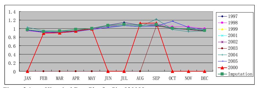
Figure 2.1 Historical Data Plot for Site 930099
Table 2.4 Imputation of Site 930099
| | MSF | | | | | | | | | | | |
|----------------|------|------|------|------|------|------|------|------|------|------|------|------|
| YEAR | JAN | FEB | MAR | APR | MAY | JUN | JUL | AUG | SEP | OCT | NOV | DEC |
| 1997 | 0.97 | 0.91 | 0.92 | 0.95 | 1.01 | 1.08 | 1.14 | 1.08 | 1.07 | 1 | 0.98 | 0.95 |
| 1998 | 0.95 | 0.91 | 0.91 | 0.94 | 0.99 | 1.04 | 1.11 | 1.07 | 1.11 | 1.04 | 1.04 | 1 |
| 1999 | 0.97 | 0.93 | 0.94 | 0.98 | 1 | 1.07 | 1.1 | 1.07 | 1.09 | 1.01 | 0.99 | 0.96 |
| 2001 | | | | | | | | | | | | |
| 2002 | | | | | | | | | | | | |
| 2003 | 0 | 0 | 0 | 0 | 0 | 0 | 0 | 0 | 1.06 | 1.02 | 0.97 | 0.94 |
| 2004 | 1.03 | 0.95 | 0.94 | 0.94 | 1.01 | 1.04 | 1.07 | 1.04 | 1.22 | 0.98 | 0.93 | 0.94 |
| 2005 | 0.96 | 0.92 | 0.9 | 0.93 | 0.98 | 1.02 | 1.07 | 1.04 | 1.06 | 1.17 | 1.03 | 0.97 |
| | | | | | | | | | | | | |
| 2000 | 0 | 0.89 | 0.9 | 0.94 | 0.99 | 0 | 0 | 1.12 | 1.13 | 0 | 0 | 0 |
| Imputed | 0.97 | 0.93 | 0.94 | 0.98 | 1 | 1.07 | 1.1 | 1.07 | 1.09 | 1.01 | 0.99 | 0.96 |
| Source
year | 1999 | 1999 | 1999 | 1999 | 1999 | 1999 | 1999 | 1999 | 1999 | 1999 | 1999 | 1999 |
**Example 2:** The October MSF borrowed from the 1999 data based on the average
For site 930174, all of the 12 MSFs for 1999 are available. However, the MSF for October 1999 is different from those from all other years. Therefore, the average value of all other years is computed as the imputed value. Figure 2.2 shows the historical data plot. Table 2.5 provides the data used and the imputed values.
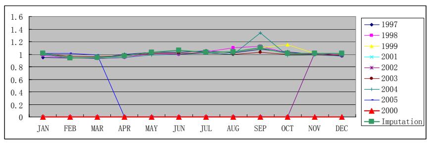
Figure 2.2 Historical Data plot of Site 930174
Table 2.5 Imputation of Site 930174
| | | | | | | | MSF | | | | | |
|---------|------|------|------|------|------|------|------|------|------|------|------|------|
| YEAR | JAN | FEB | MAR | APR | MAY | JUN | JUL | AUG | SEP | OCT | NOV | DEC |
| 1997 | 0.95 | 0.94 | 0.94 | 1 | 1.03 | 1.03 | 1.05 | 1.02 | 1.08 | 1.04 | 1 | 0.97 |
| 1998 | 0.98 | 0.94 | 0.93 | 0.95 | 1.01 | 1 | 1.04 | 1.1 | 1.13 | 1.02 | 1 | 0.98 |
| 1999 | 1.01 | 0.94 | 0.95 | 0.97 | 1.03 | 1.06 | 1.03 | 1.04 | 1.1 | 1.15 | 1.01 | 1.01 |
| 2001 | | | | | | | | | | | | |
| 2002 | 0 | 0 | 0 | 0 | 0 | 0 | 0 | 0 | 0 | 0 | 1.02 | 0.98 |
| 2003 | 1.01 | 0.96 | 0.96 | 0.97 | 1.01 | 1.01 | 1.02 | 1 | 1.03 | 1 | 1 | 0.99 |
| 2004 | 1 | 0.95 | 0.93 | 0.95 | 0.99 | 1 | 1.02 | 1 | 1.34 | 0.98 | 0.99 | 0.97 |
| 2005 | 1.01 | 1.01 | 0.99 | 0 | 0 | 0 | 0 | 0 | 0 | 0 | 0 | 0 |
| | | | | | | | | | | | | |
| 2000 | 0 | 0 | 0 | 0 | 0 | 0 | 0 | 0 | 0 | 0 | 0 | 0 |
| Imputed | 1.01 | 0.94 | 0.95 | 0.97 | 1.03 | 1.06 | 1.03 | 1.04 | 1.1 | 1.01 | 1.01 | 1.01 |
| Source | | | | | | | | | | | | |
| year | 1999 | 1999 | 1999 | 1999 | 1999 | 1999 | 1999 | 1999 | 1999 | Avg. | 1999 | 1999 |
**Example 3:** The entire year 2001 data borrowed
For site 740047, data for four months in 2000 are missing. The 1999 data are also missing for several months and cannot be used. As a result, the 2001 data are borrowed. Figure 2.3 shows that seasonal patterns are similar for the period between 1997 and 2005. Table 2.6 gives the imputation results.
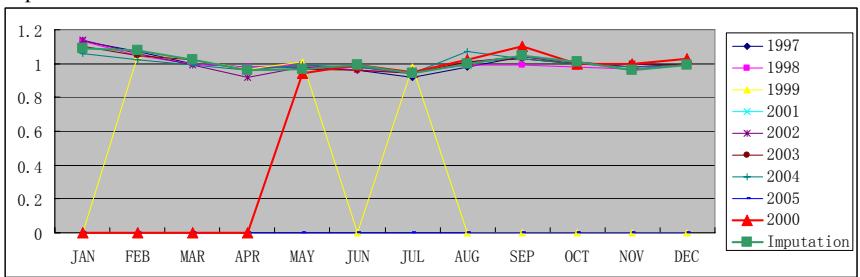
Figure 2.3 Historical Data Plot for Site 740047
Table 2.6 Imputation of Site 740047
| | | | | | | | MSF | | | | | |
|---------|------|------|------|------|------|------|------|------|------|------|------|------|
| YEAR | JAN | FEB | MAR | APR | MAY | JUN | JUL | AUG | SEP | OCT | NOV | DEC |
| 1997 | 1.13 | 1.07 | 1 | 0.98 | 0.98 | 0.96 | 0.92 | 0.98 | 1.04 | 1.01 | 0.98 | 1 |
| 1998 | 1.13 | 1.05 | 1 | 0.98 | 0.99 | 0.96 | 0.95 | 0.99 | 0.99 | 0.98 | 0.97 | 1 |
| 1999 | 0 | 1.05 | 1.02 | 0.97 | 1.01 | 0 | 0.98 | 0 | 0 | 0 | 0 | 0 |
| 2001 | 1.09 | 1.08 | 1.02 | 0.96 | 0.97 | 0.99 | 0.94 | 1 | 1.05 | 1.01 | 0.96 | 0.99 |
| 2002 | 1.14 | 1.06 | 0.99 | 0.92 | 0.98 | 0.98 | 0.94 | 1.01 | 1.04 | 1 | 1 | 0.99 |
| 2003 | 1.1 | 1.05 | 1.02 | 0.96 | 0.97 | 0.96 | 0.94 | 1.01 | 1.03 | 1 | 1 | 0.99 |
| 2004 | 1.06 | 1.02 | 0.99 | 0.96 | 0.99 | 0.98 | 0.94 | 1.07 | 1.03 | 1 | 0.98 | 0.99 |
| 2005 | 0 | 0 | 0 | 0 | 0 | 0 | 0 | 0 | 0 | 0 | 0 | 0 |
| | | | | | | | | | | | | |
| 2000 | 0 | 0 | 0 | 0 | 0.94 | 0.99 | 0.95 | 1.02 | 1.1 | 1 | 1 | 1.03 |
| Imputed | 1.09 | 1.08 | 1.02 | 0.96 | 0.97 | 0.99 | 0.94 | 1 | 1.05 | 1.01 | 0.96 | 0.99 |
| Source | | | | | | | | | | | | |
| year | 2001 | 2001 | 2001 | 2001 | 2001 | 2001 | 2001 | 2001 | 2001 | 2001 | 2001 | 2001 |
### **2.4 Data Imputation Results**
For the 69 TTMSs with missing data in 2000, the MSFs for 54 sites are imputed successfully. The remaining 15 sites cannot be imputed for the following reasons:
- (1) Three sites do not have reliable historical data.
- (2) Three sites show inconsistent patterns in the historical data.
- (3) Two sites are co-located with other sites.
- (4) Seven sites have no MSF data for all of the years.
These 15 sites are excluded from the datasets used for analyses. Table 2.7 lists these sites and gives the reasons for unsuccessful imputation in the last column. "C" indicates that a TTMS is co-located with another TTMS. Therefore, it is not needed. "U" indicates unreliable historical data. "M" means no data are available. "V" means that there are large variations in the historical data.
Table 2.7 List of TTMS with Missing Data after Imputation
| Index | SITE | Description | Reason | |
|-------|--------|----------------------------------------------------|--------|--|
| 1 | 019917 | US41, 4.8 MI N OF LEE CO (NEAR R 14, 1000 & 117) | C | |
| 2 | 100338 | SR583 (56TH ST), 1216 FT S OF SLIGH AVE - HILLS#03 | U | |
| 3 | 100339 | SR60 (CC CSWY), 1996 FT W ROCKY PT DR - HILLS#18 | U | |
| | | SR674-COLLEGE AV, 285 FT W CYPRESS V BLVD | | |
| 4 | 100341 | HILLS#53 | U | |
| | | I-75/SR-93, 3 MILES NORTH OF MARION COUNTY | | |
| 5 | 269904 | LINE | V | |
| 6 | 550201 | US-319(CAPITAL CIRCLE), 0.3 MI. EAST OF SR-61 | C | |
| | | I-10/SR-8, APPROX. 1.3 MI. WEST OF BOY SCOUT | | |
| 7 | 609928 | ROAD | V | |
| 8 | 799906 | I-4, 0.4 MI E ENTERPRISE RD OP REPL TTMS 0179 | V | |
| 9 | 079918 | SR 25/80, US 27 1.6 MI EAST OF SR 80
R-160 | M | |
| 10 | 100342 | SR45/US41, 574 FT N OF TRENTON ST - HILLS#58 | M | |
| | | I10 JEFFERSON CO, APPROX 1.0 MI E OF SR257, | | |
| 11 | 549901 | WIM#1 | M | |
| 12 | 720157 | I-295,3.0 MI N OF I-10,WIM#14 UC 9/94 | M | |
| | | SR 834/SAMPLE RD. 0.14 MI.W OF NW 14TH AVE. | | |
| 13 | 860255 | TTMS | M | |
| | | SR 818/GRIFFIN RD, 112' WEST OF SW 70TH AVE. | | |
| 14 | 860256 | TTMS | M | |
| | | I-4/SR-400, APPROX. 0.4 MI. SW OF ORANGE CTY. | | |
| 15 | 920303 | LINE | M | |
| | | | | |
"C": Co-located with another site.
"U": Historical data are unreliable.
"M": Not included in MSF dataset.
"V": Cannot be imputed as large variation in historical data.
### **3. SEASONAL FACTOR GROUPING**
This chapter presents the seasonal factor grouping for urban and rural areas. The grouping can be used later for short-term count site assignment to seasonal factor groups. The groups may also provide clues as what geographic areas might share similar land use characteristics.
All of the TTMSs are classified as urban and rural sites according to the map provided on the FDOT 2000 Traffic Information CD. The map is shown in Figure 3.1. Grouping is performed for the urban and rural TTMSs separately.
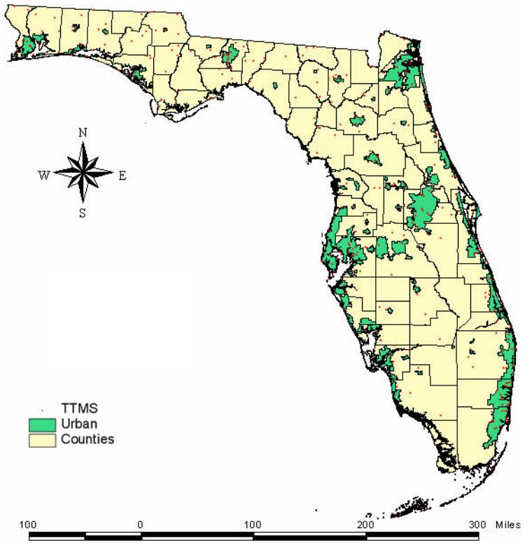
Figure 3.1 Urban and Rural Area Definition
The creation of seasonal factors groups involved both cluster analyses and manual adjustments. The statistical methods available include hierarchical cluster analysis and model-based cluster analysis methods. These methods group the TTMSs based on the similarity between their MSFs. Compared with the hierarchical cluster method, model-based cluster analysis gives the grouping result as well as the optimal number of groups. Thus, the model-based cluster analysis method is adopted to determine grouping.
Different sets of variables are also tested for model-based cluster analysis. These include:
- 12 MSFs only;
- 12 MSFs and 2 location variables (longitude and latitude);
- 12 MSFs and 11 slope variables (11 differences between two adjacent months' seasonal factor).
When the location variables, expressed as the longitude and latitude of the TTMSs, are included in the cluster analysis, the optimal group number grows significantly. A comparison of the results obtained by using the above sets of variables will be given in Sections 3.1.1 and 3.2.1.
The 11 slope variables represent the direction of change in MSF from one month to the next. The purpose is not only to group TTMSs that have similar MSFs, but also to make them similar in the direction of the changes. Therefore, 11 slope variables (difference between MSF of one month and that of the previous month) plus the 12 MSFs are used in the cluster analysis. However, the introduction of the slope variables only slightly improved the cluster results and only for urban TTMSs. The results obtained using the 12 MSFs as the variables and the results using the 23 variables are compared in Table 3.1 and Table 3.2, respectively, for urban and rural TTMSs. The comparison is made based on the following three measures of effectiveness:
• The average squared deviation of the 12 MSFs for all sites, which is the sum of the 12 squared distances between MSFs for each site, and the average MSFs for the group:
$$D = \frac{\sum_{j=1}^{N} \sum_{i=1}^{12} \left( MSF_{ji} - \overline{MSF}_{i} \right)^{2}}{N}$$
(3-1)
where
*D* = the average squared deviation of MSFs
*MSFji* = the monthly seasonal factor for month *i* and TTMS *j*,
*MSFj* = the group average MSF for month *i*,
*N* = the number of TTMSs in each group.
- The number of months for which the MSFs exceed the threshold of 5% of the group average.
- The number of TTMSs for which the MSFs exceed the threshold of 5% of the group average.
The smaller the values of these measurements are, the better the result is.
Table 3.1 Comparison of MOE for Urban Area
| Group Size | D | # Months over 5% | # TTMSs over 5% |
|------------|--------|------------------|-----------------------------------|
| 5 | 0.0257 | 15 | 5 |
| 10 | 0.0150 | 17 | 8 |
| 5 | 0.0168 | 14 | 5 |
| 32 | 0.0072 | 15 | 10 |
| 32 | 0.0062 | 15 | 10 |
| 19 | 0.0135 | 27 | 10 |
| 4 | 0.0172 | 8 | 3 |
| 1 | NA | NA | NA |
| 4 | 0.0104 | 5 | 2 |
| 11 | 0.0097 | 10 | 6 |
| 123 | 0.1217 | 126 (8.54%) | 59 (47.97%) |
| | | | |
| 9 | 0.0247 | 26 | 8 |
| 12 | 0.0092 | 9 | 6 |
| 27 | 0.0077 | 13 | 8 |
| 6 | 0.0206 | 13 | 6 |
| 5 | 0.0201 | 10 | 3 |
| 1 | NA | NA | NA |
| | | | 3 |
| 17 | 0.0123 | 20 | 9 |
| 31 | 0.0057 | 13 | 10 |
| 10 | 0.0080 | 6 | 4 |
| 123 | 0.1220 | 119 (8.06%) | 57 (46.34%) |
| | 5 | 0.0136 | 12 Variables
23 Variables
9 |
Table 3.2 Comparison of MOE for Rural Area
| | | | 12 Variables | |
|-------|------------|--------|------------------|-----------------|
| Group | Group Size | D | # Months over 5% | # TTMSs over 5% |
| 1 | 28 | 0.0165 | 52 | 17 |
| 2 | 5 | 0.0164 | 9 | 4 |
| 3 | 2 | 0.0271 | 6 | 2 |
| 4 | 27 | 0.0126 | 38 | 20 |
| 5 | 13 | 0.0143 | 21 | 10 |
| 6 | 42 | 0.0123 | 47 | 23 |
| 7 | 12 | 0.0272 | 32 | 10 |
| 8 | 12 | 0.0205 | 29 | 7 |
| 9 | 6 | 0.0268 | 18 | 5 |
| SUM | 147 | 0.1736 | 252 (14.29%) | 98 (66.67%) |
| | | | 23 Variables | |
| 1 | 10 | 0.0190 | 16 | 6 |
| 2 | 26 | 0.0139 | 45 | 16 |
| 3 | 22 | 0.0195 | 50 | 17 |
| 4 | 2 | 0.0271 | 6 | 2 |
| 5 | 22 | 0.0140 | 31 | 14 |
| 6 | 36 | 0.0111 | 40 | 20 |
| 7 | 10 | 0.0154 | 18 | 8 |
| 8 | 7 | 0.0347 | 28 | 6 |
| 9 | 12 | 0.0282 | 32 | 10 |
| SUM | 147 | 0.1828 | 266 (15.08%) | 99 (67.35%) |
Based on the above discussion, model-based cluster analysis with only 12 MSFs as the variables is used for grouping the TTMSs. This is followed by manual adjustment of the seasonal factor groups. Note that the results from the model-based cluster analysis with the location variables are also used as a reference during the manual adjustment process. The adjustment is made based on the following general rules:
- (1) Groups with TTMSs located in the same geographic area and sharing similar MSF patterns remain unchanged.
- (2) A groups is subdivided in the following two cases:
- (a) The TTMSs within a group are geographically separated by a long distance, or there is a significant difference in their latitudes. The latter may mean a significant difference in climate. For instance, a TTMS located in South Florida will not be grouped together with one in Jacksonville.
- (b) The MSFs of some TTMSs have a different pattern from that of the others within the same group.
The grouping results are described in greater detail in the following sections.
### **3.1 Seasonal Factor Grouping for Urban Areas**
Of the 270 TTMS, 128 are in urban areas. The model-based cluster analysis without considering the locations resulted in 10 groups.
Table 3.3 Comparison of Cluster Analyses for Urban TTMSs
| Method | Number of Groups |
|--------------------------|------------------|
| Model based without X, Y | 10 |
| Model based with X, Y | 33 |
### 3.1.1 Results from Cluster Analysis in Urban Areas
The grouping results from model-based clustering method for the TTMSs located in urban areas, without incorporating the X and Y coordinates, are shown in Figure 3.2. The model produces ten clusters that include TTMSs that are far apart when the location effect is not considered. While some TTMSs that are far away from each other may share similar seasonal traffic patterns, the underlying causes may be quite different due to differences in climate, population characteristics, economic structures, etc.
Table 3.4 gives the number of TTMSs in each group. Nine out of the ten groups consist of more than one TTMS.
Table 3.4 Number of TTMS Stations in the Optimal Ten Urban Groups
| Group | Number of TTMS Stations |
|-------|-------------------------|
| 1 | 2 |
| 2 | 12 |
| 3 | 4 |
| 4 | 34 |
| 5 | 3 |
| 6 | 45 |
| 7 | 9 |
| 8 | 5 |
| 9 | 1 |
| 10 | 8 |
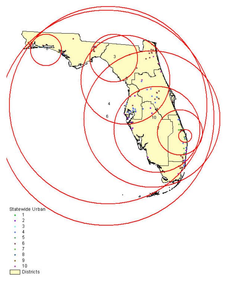
Figure 3.2 Optimal Ten Groups from Model-Based Method for Urban Areas
Model-based clustering is also performed with the location of the TTMSs considered. In other words, the clusters are produced by simultaneously considering the similarity in the monthly seasonal factors, as well as the proximity of the TTMSs. The spatial distribution of the groups is depicted in Figure 3.3. The figure reveals a more spatially clustered pattern of the TTMSs. However, as shown in Table 3.5, 33 groups are created, compared to 10 when location is not considered. Furthermore, many groups are made up by a single TTMS station, which is undesirable.
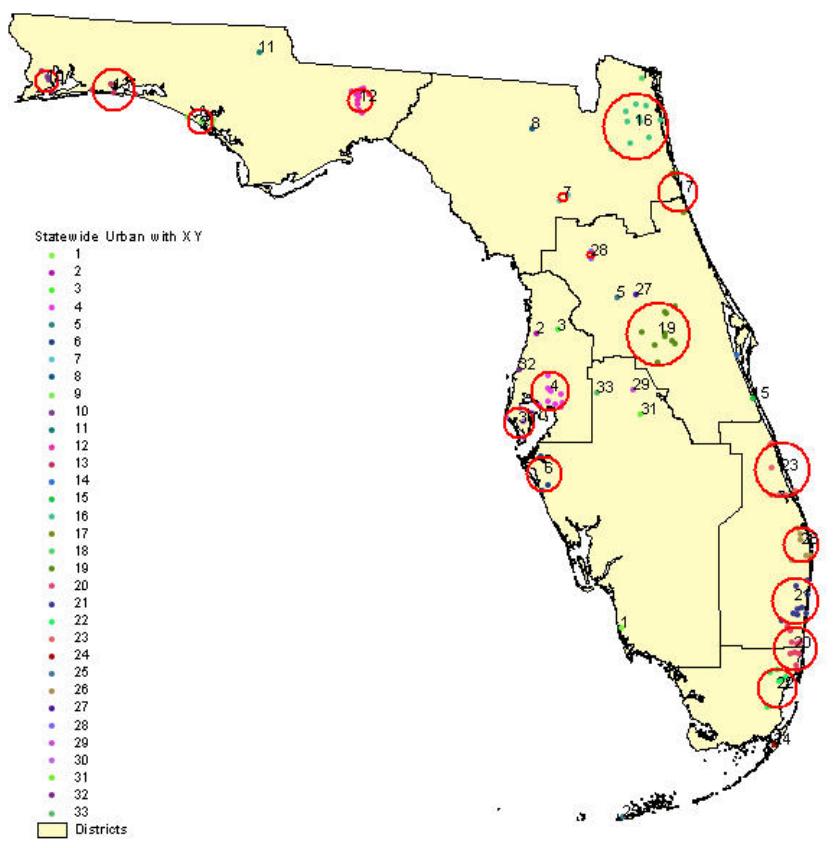
Figure 3.3 Optimal 33 Groups for Urban Areas from the Model-Based Method with Location Variables Included
Table 3.5 Number of TTMS Stations in the Optimal 33 Urban Groups from Model-Based Cluster Analysis with Location Variables
| Group | Number of TTMSs |
|-------|-----------------|
| 1 | 1 |
| 2 | 1 |
| 3 | 1 |
| 4 | 9 |
| 5 | 1 |
| 6 | 3 |
| 7 | 2 |
| 8 | 1 |
| 9 | 4 |
| 10 | 4 |
| 11 | 1 |
| 12 | 11 |
| 13 | 4 |
| 14 | 1 |
| 15 | 1 |
| 16 | 10 |
| 17 | 3 |
| 18 | 1 |
| 19 | 10 |
| 20 | 12 |
| 21 | 9 |
| 22 | 6 |
| 23 | 7 |
| 24 | 1 |
| 25 | 1 |
| 26 | 6 |
| 27 | 1 |
| 28 | 2 |
| 29 | 1 |
| 30 | 5 |
| 31 | 1 |
| 32 | 1 |
| 33 | 1 |
The results shown in Table 3.5 suggest that the model-based cluster method with x-y coordinates added may not be appropriate for clustering the urban TTMSs statewide. This is because location seems to be given too great a weight. For example, Palm Beach County may share some similarities with counties along the southwest Gulf Coast in terms of climate and population characteristics. However, they will not be grouped together, even if their MSF patterns are similar, simply because they are spatially separated. As one of the objectives of the research is to identify variables that potentially influence the seasonal patterns of traffic, a small number of groups is more desirable than a large number of groups. This is because more groups mean greater complexity.
It is easier to divide fewer groups into more groups based on the similarity of MSF patterns within a group than it is to merge smaller groups into larger ones. Hence, the results from cluster analysis, without considering location (as shown in Figure 3.2 and Table 3.4), are used as the basis to refine the grouping. This process is manual and involves inspecting each group and identifying TTMSs that do not belong. Also note that, for practical applications, jurisdiction is also important when creating seasonal factor groups. The boundary of FDOT districts are also considered when refining the grouping. The results are described in the next section.
### 3.1.2 Refinement of Cluster Results for Urban Areas
The grouping results shown in Figure 3.2 are further investigated. Figures 3.4 through 3.8 show the spatial distribution patterns and MSF profiles for TTMS Groups 1, 3, 7, 8, and 9, respectively. The figures demonstrate that the TTMSs in the same group have similar monthly profiles and are located in close proximity. In the profiles, the red lines indicate the 5% thresholds above and below the group means.
The TTMSs in the above groups are identified in Table 3.6.
Table 3.6 TTMSs in Urban Groups 1, 3, 7, 8, and 9
| Group | Number of TTMSs | TTMSs |
|-------|-----------------|------------------------------------------------------------------------------------|
| 1 | 2 | C890259, C930087 |
| 3 | 4 | C260323, C550208, C550209, C550226 |
| 7 | 9 | C700114, C860214, C940260, C940334, C970410,
C970413, C970416, C970417, C979913 |
| 8 | 5 | C460305, C570293, C580261, C570167, C600168 |
| 9 | 1 | C460166 |
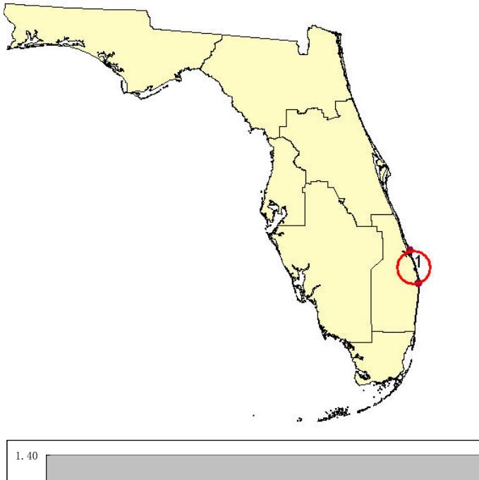
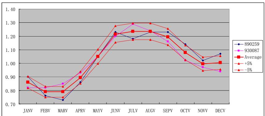
Figure 3.4 Spatial Distribution and Profiles of the TTMSs in Urban Group 1
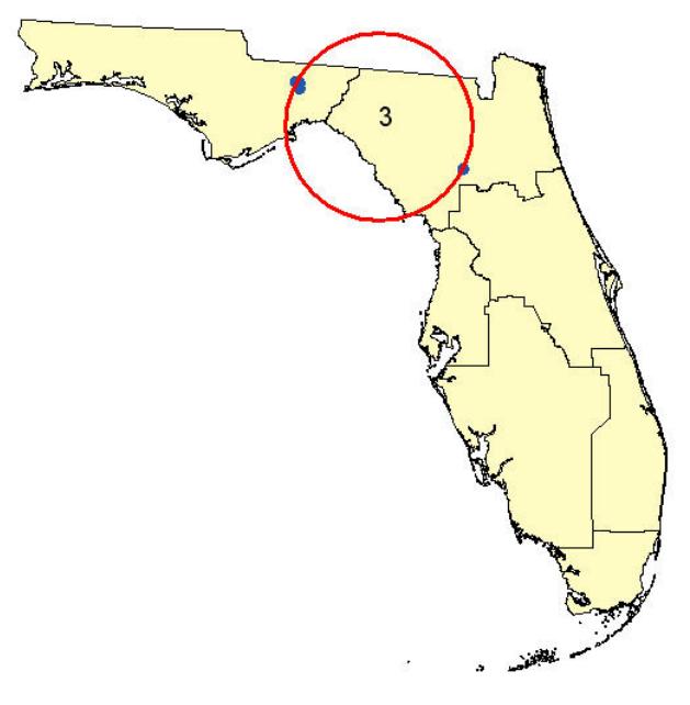
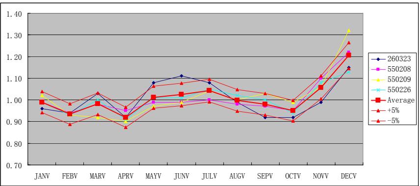
Figure 3.5 Spatial Distribution and Profiles of the TTMSs in Urban Group 3
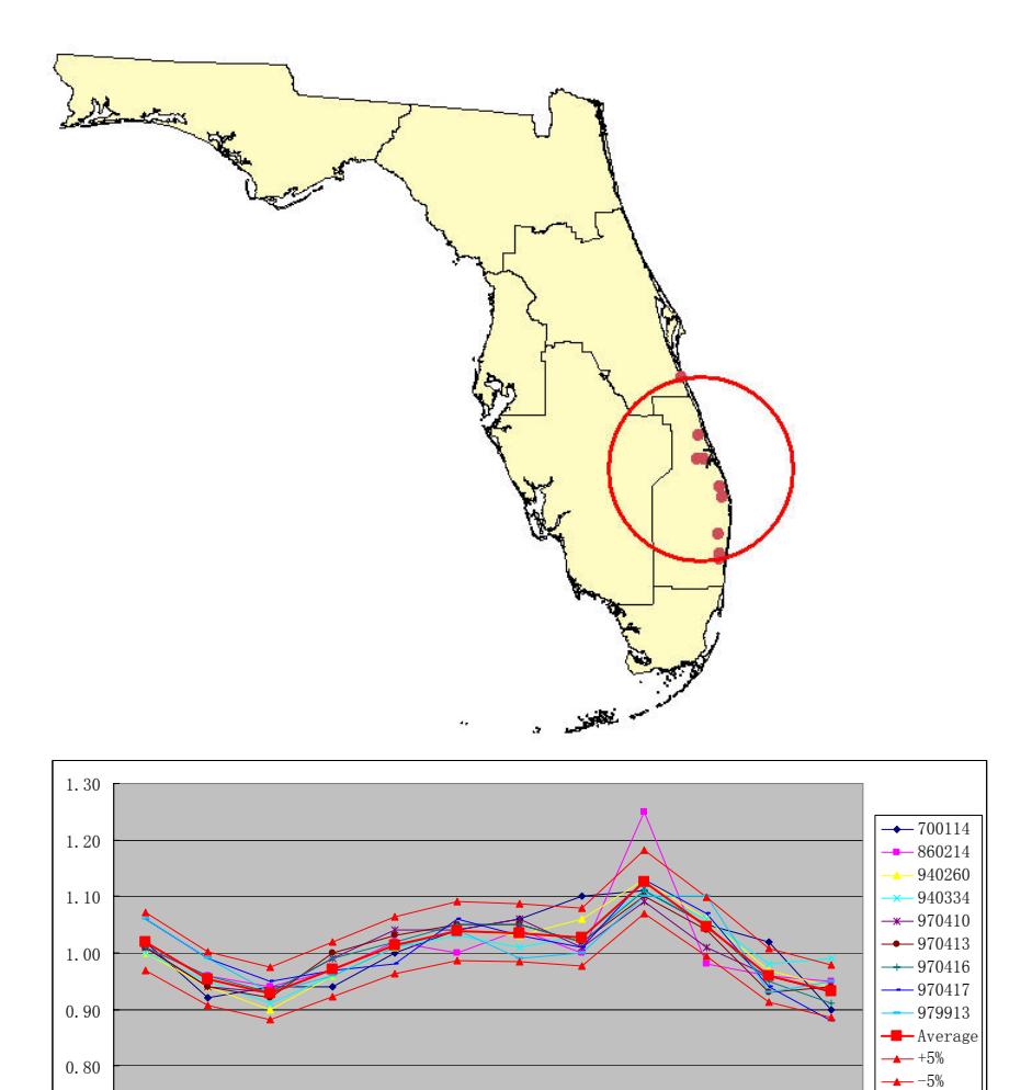
Figure 3.6 Spatial Distribution and Profiles of the TTMSs in Urban Group 7
JANV FEBV MARV APRV MAYV JUNV JULV AUGV SEPV OCTV NOVV DECV
0.70
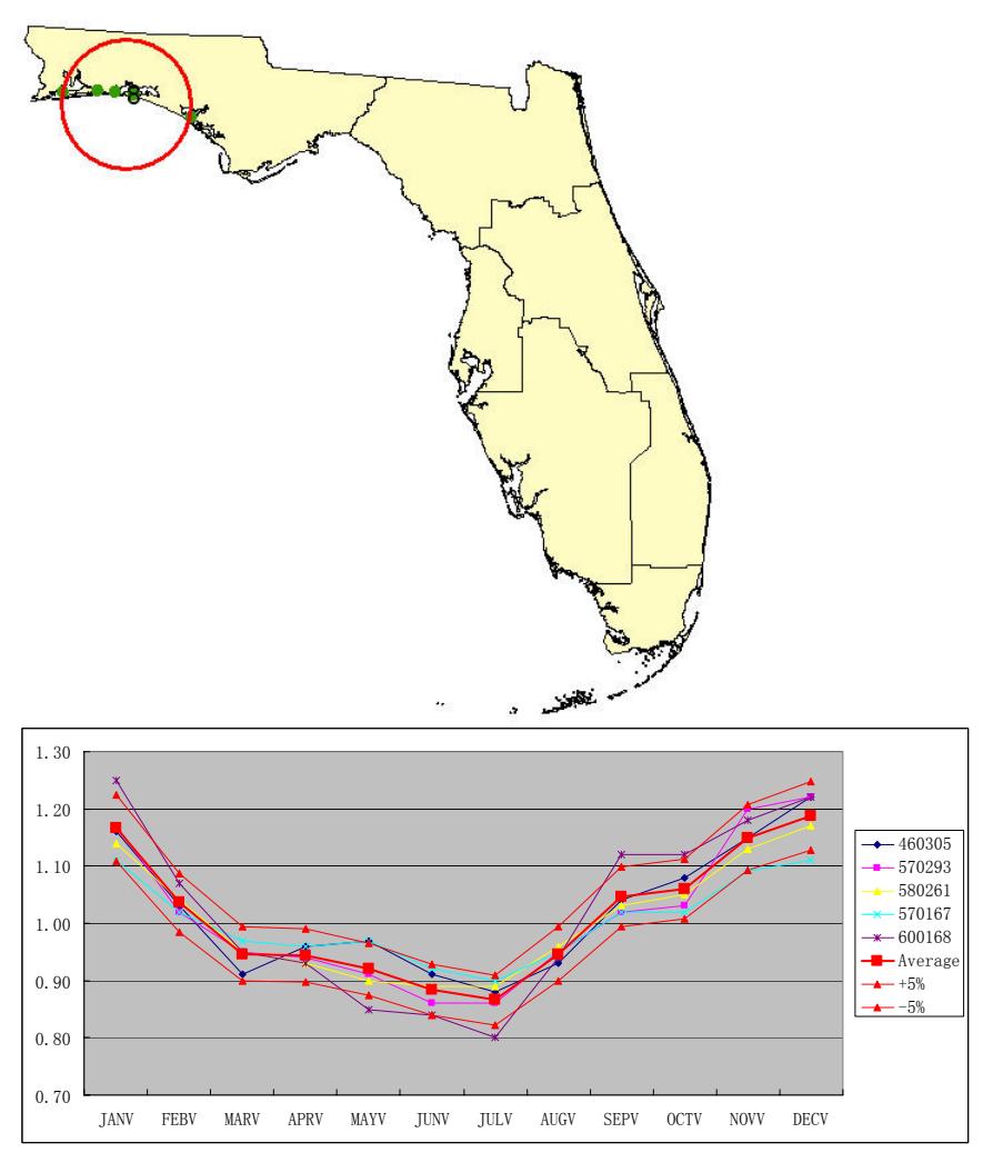
Figure 3.7 Spatial Distribution and Profiles of the TTMSs in Urban Group 8
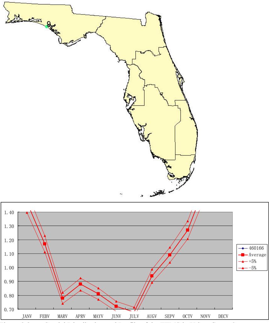
Figure 3.8 Spatial Distribution and Profile of the TTMS in Urban Group 9
For Groups 2, 4, 5, 6, and 10, the TTMSs in the same group are located far apart. For example, as shown in Figure 3.9, the TTMSs in Group 2 span over four FDOT districts. The TTMSs in this group are reassigned to three new groups (Groups 21, 22, and 23) as shown in Figure 3.10. The group profiles are depicted in Figures 3.11 through 3.13.
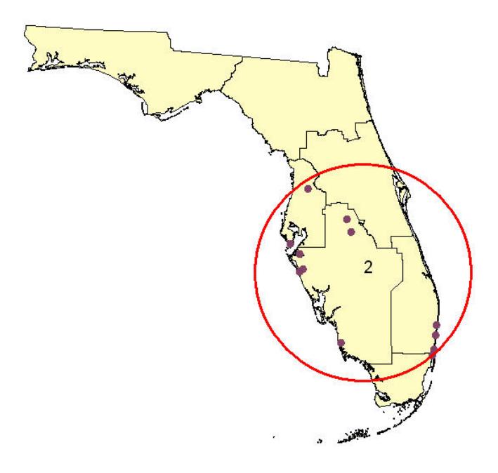
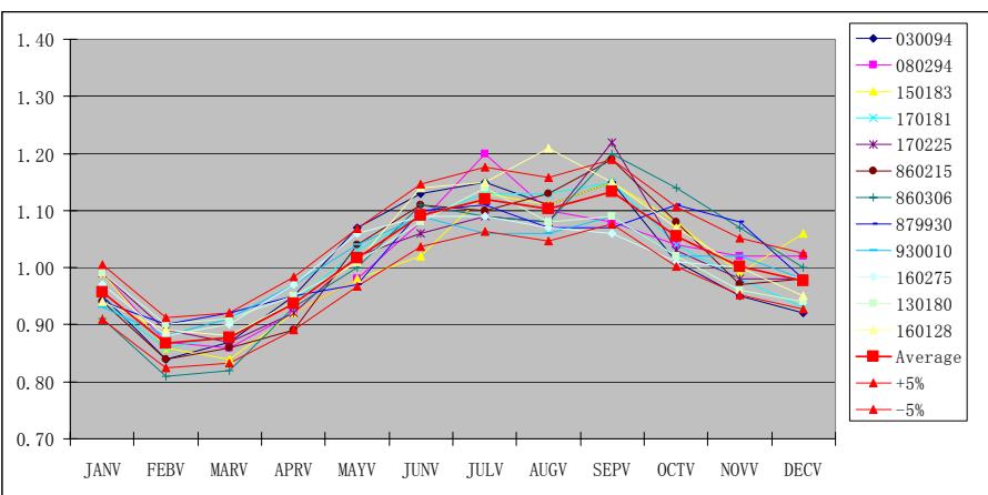
Figure 3.9 Spatial Distribution and Profiles of the TTMSs in Urban Group 2
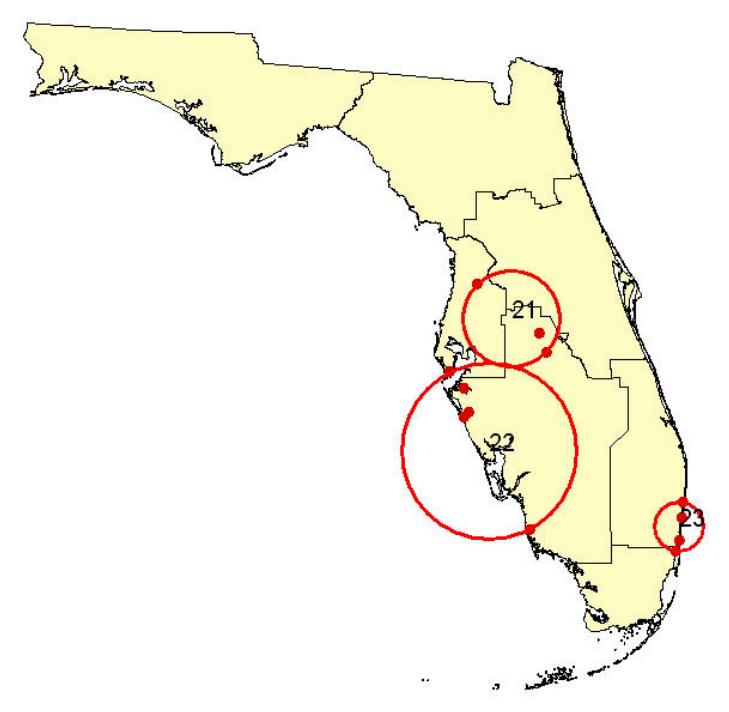
Figure 3.10 Spatial Distribution of the Three New Subgroups for the Urban Group 2
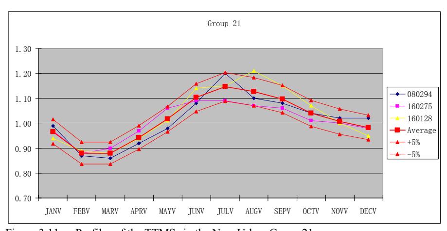
Figure 3.11 Profiles of the TTMSs in the New Urban Group 21
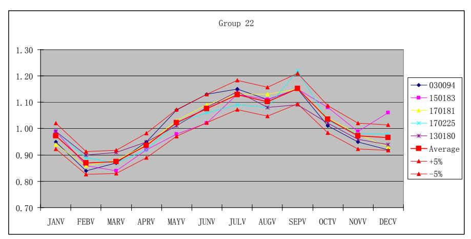
Figure 3.12 Profiles of the TTMSs in the New Urban Group 22
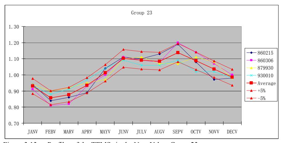
Figure 3.13 Profiles of the TTMSs in the New Urban Group 23
The TTMSs in Group 4, as illustrated in Figure 3.14, are spread over nearly the entire state. Similar to Group 2, the TTMSs in Group 4 are split into three new subgroups: 41, 42, and 43, as shown in Figure 3.15. The group profiles are plotted in Figures 3.16 through 3.18.
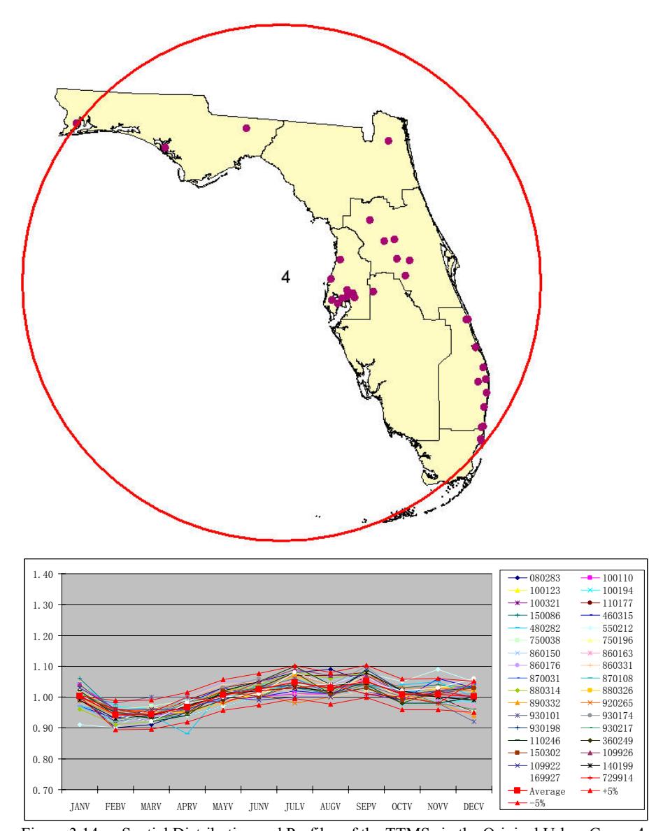
Figure 3.14 Spatial Distribution and Profiles of the TTMSs in the Original Urban Group 4
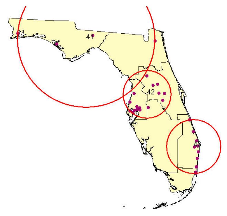
Figure 3.15 Spatial Distribution of the Three New Subgroups for the Original Urban Group 4
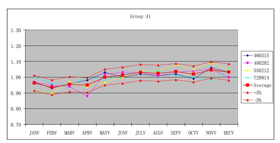
Figure 3.16 Profiles of the TTMSs in the New Urban Group 41
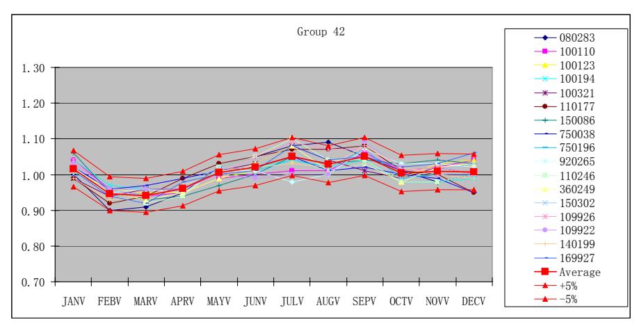
Figure 3.17 Profiles of the TTMSs in the New Urban Group 42
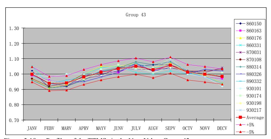
Figure 3.18 Profiles of the TTMSs in the New Urban Group 43
Figure 3.19 shows the spatial distribution of TTMSs in Group 5 and the profiles of their MSFs. Figure 3.20 illustrates the two new subgroups created from Group 5. The group profiles for the two new subgroups are shown in Figures 3.12 and 3.22.
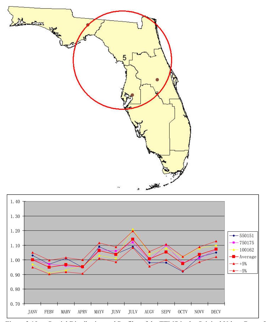
Figure 3.19 Spatial Distribution and Profiles of the TTMS in the Original Urban Group 5
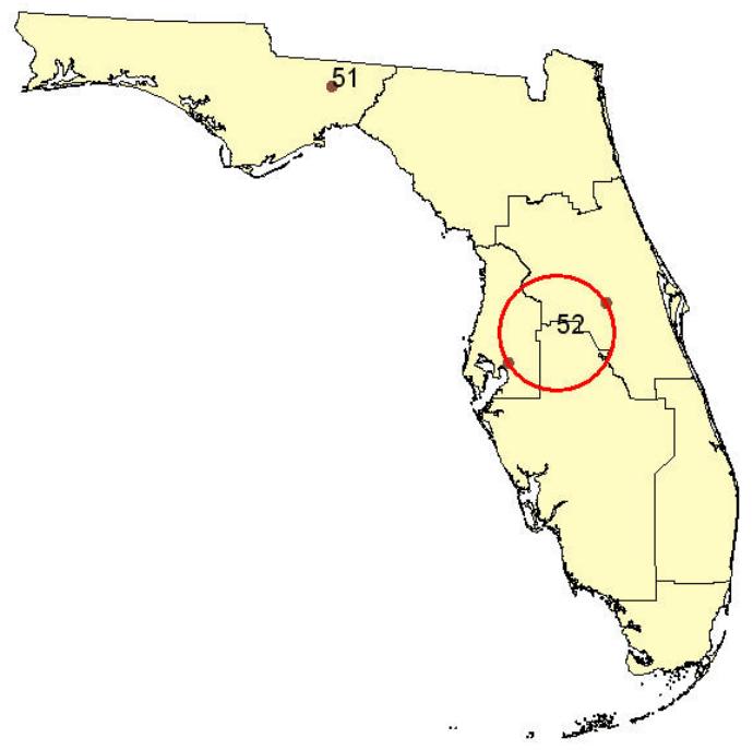
Figure 3.20 Spatial Distribution of the Two New Subgroups for the Original Urban Group 5
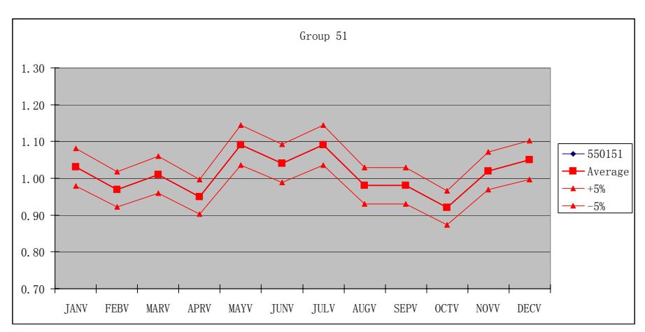
Figure 3.21 Profiles of the TTMSs in the New Urban Group 51
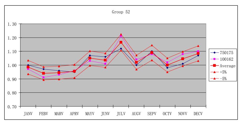
Figure 3.22 Profiles of the TTMSs in the New Urban Group 52
Figure 3.23 shows the spatial distribution of the TTMSs in Group 6 and their MSF profiles. Figure 3.24 shows the three new subgroups created from Group 6. The group profiles for the four new subgroups are depicted in Figures 3.25 through 3.28. There is a possibility that subgroups 61 and 62 may be combined.
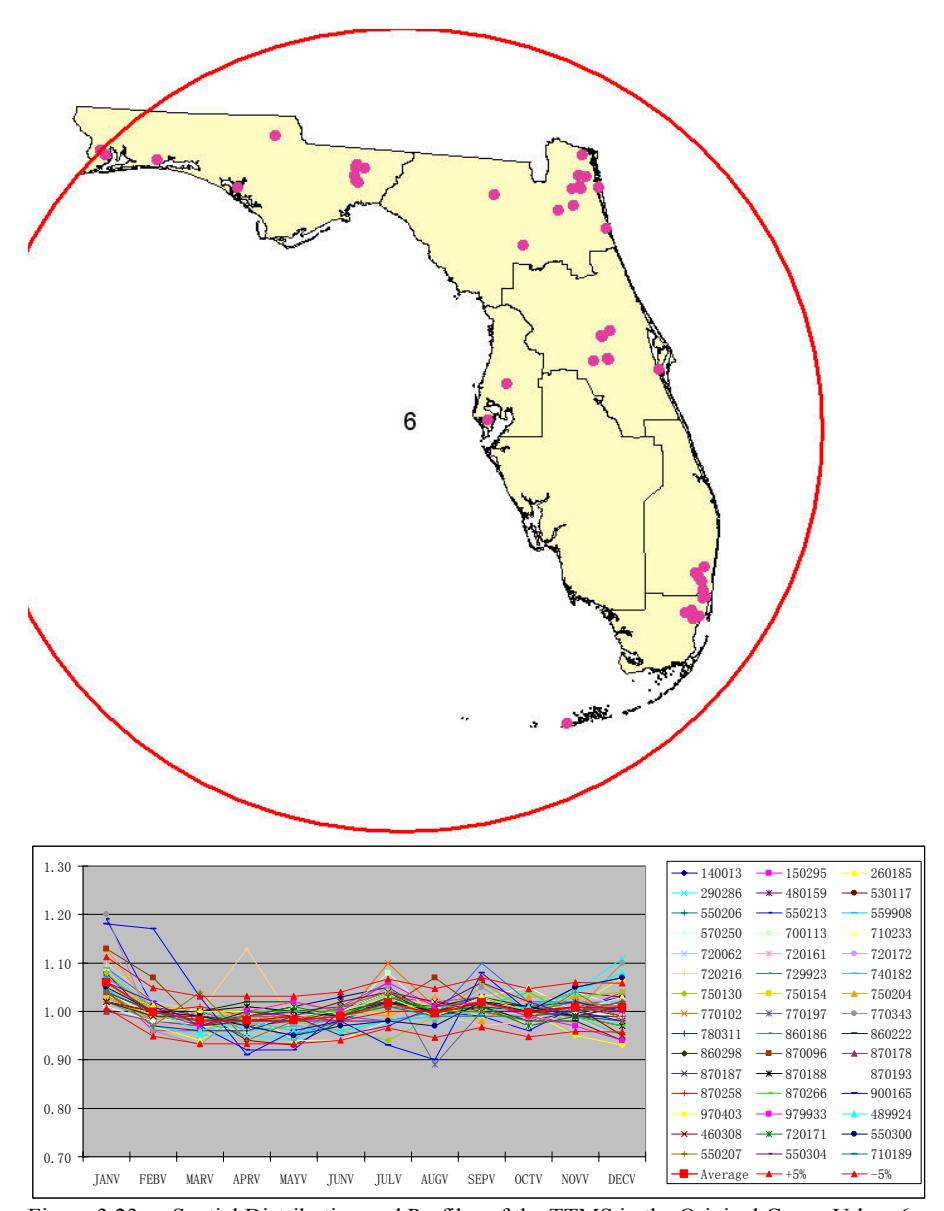
Figure 3.23 Spatial Distribution and Profiles of the TTMS in the Original Group Urban 6
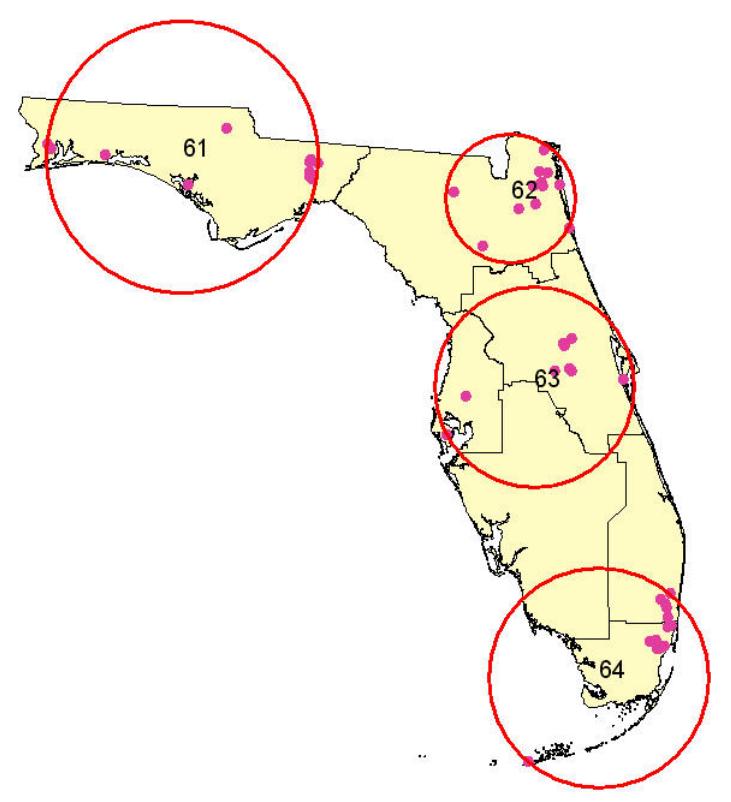
Figure 3.24 Spatial Distribution of the Four New Subgroups for the Original Urban Group 6
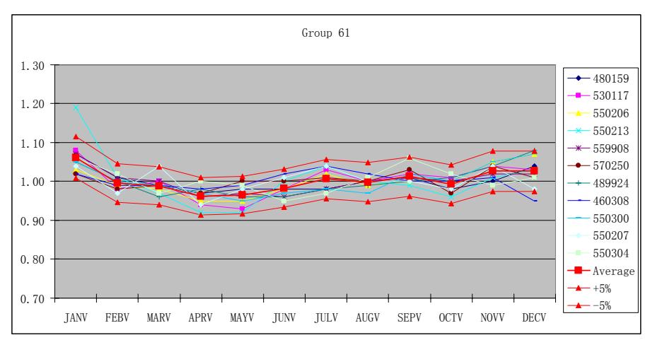
Figure 3.25 Profiles of the TTMSs in the New Urban Group 61
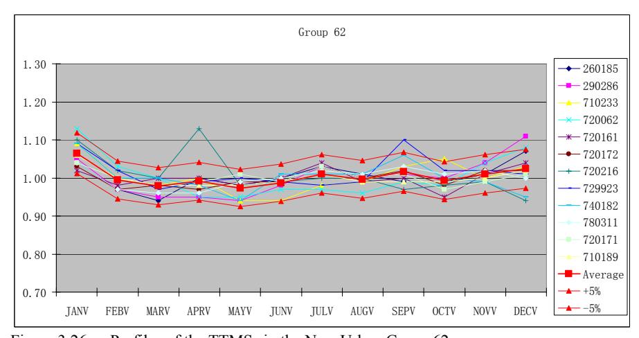
Figure 3.26 Profiles of the TTMSs in the New Urban Group 62
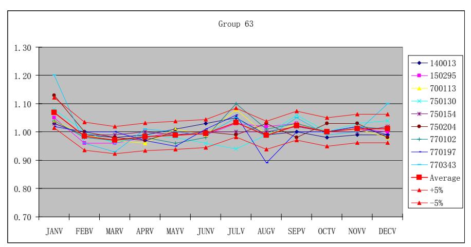
Figure 3.27 Profiles of the TTMSs in the New Urban Group 63
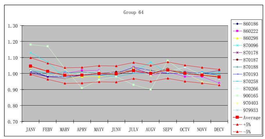
Figure 3.28 Profiles of the TTMSs in the New Urban Group 64
Finally, Group 10, as illustrated in Figure 3.29, is divided into three new subgroups. They are illustrated in Figure 3.30. The group profiles for the three new subgroups are given in Figures 3.31 through 3.33.
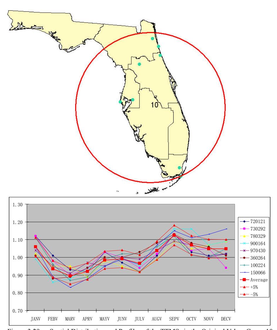
Figure 3.29 Spatial Distribution and Profiles of the TTMSs in the Original Urban Group 10
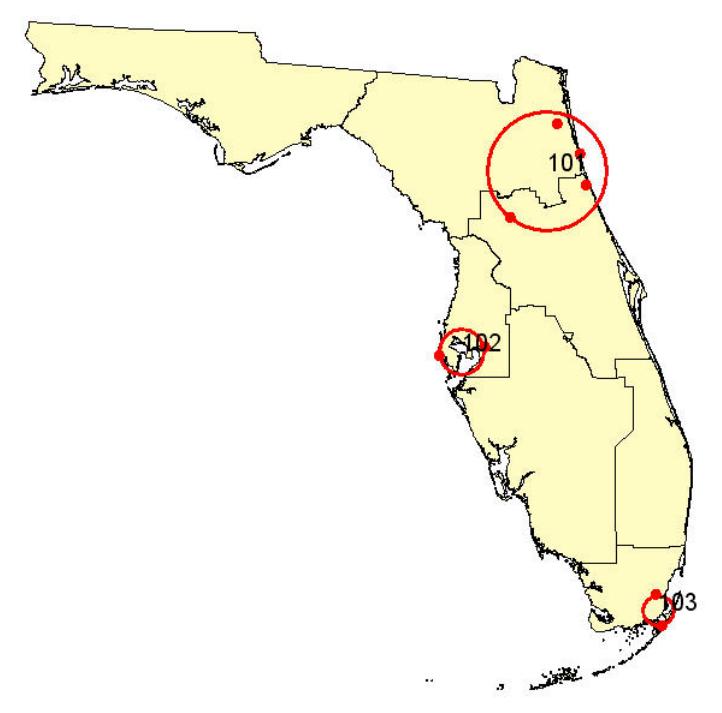
Figure 3.30 Spatial Distribution of the Three New Subgroups for the Original Urban Group 10
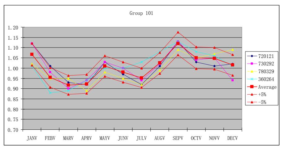
Figure 3.31 Profiles of the TTMSs in the New Urban Group 101
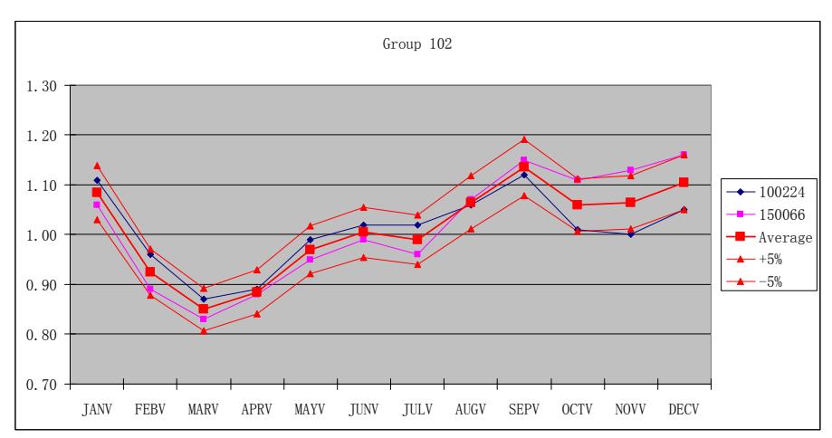
Figure 3.32 Profiles of the TTMSs in the New Urban Group 102
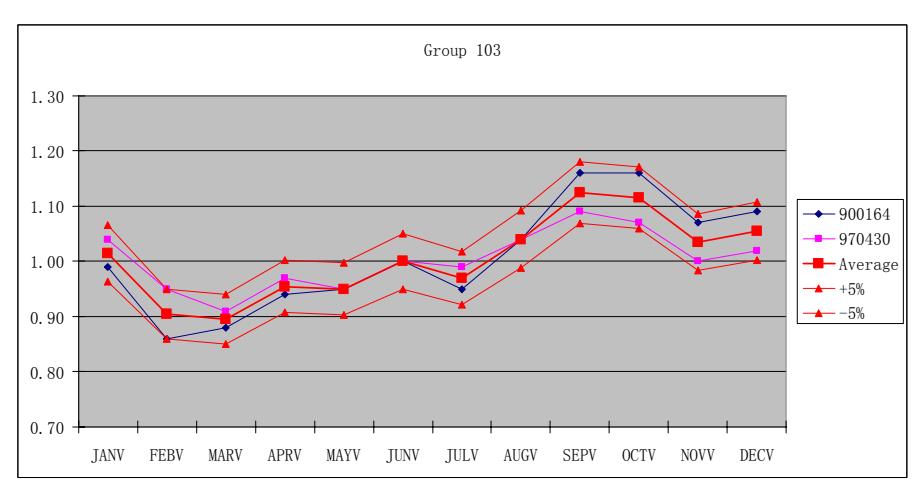
Figure 3.33 Profiles of the TTMSs in the New Urban Group 103
After the TTMSs in Groups 2, 4, 5, 6 and 10 are reassigned, a total of 20 seasonal groups are defined for the 123 TTMSs located in the urban area. Figure 3.34 shows the spatial patterns of the TTMSs in these 20 TTMS groups. The number of stations in each group is presented in Table 3.7.
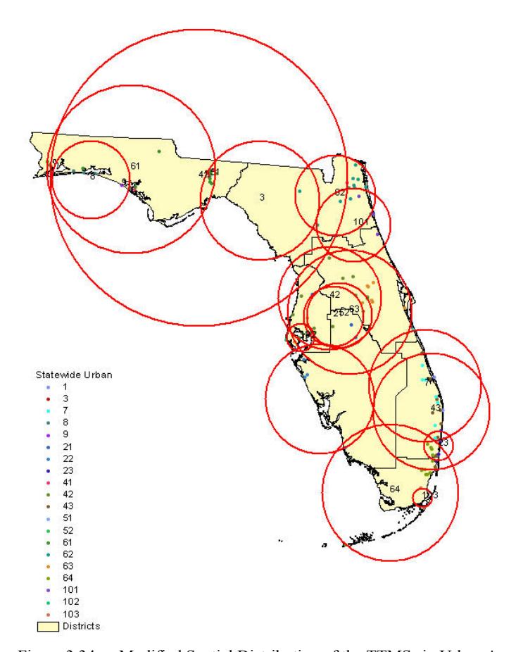
Figure 3.34 Modified Spatial Distribution of the TTMSs in Urban Areas
Table 3.7 Number of the TTMSs in the 20 Urban Groups
| Group | Number of TTMSs |
|-------|-----------------|
| 1 | 2 |
| 3 | 4 |
| 7 | 9 |
| 8 | 5 |
| 9 | 1 |
| 21 | 3 |
| 22 | 5 |
| 23 | 4 |
| 41 | 4 |
| 42 | 17 |
| 43 | 13 |
| 51 | 1 |
| 52 | 2 |
| 61 | 11 |
| 62 | 12 |
| 63 | 9 |
| 64 | 13 |
| 101 | 4 |
| 102 | 2 |
| 103 | 2 |
| | |
### **3.2 Seasonal Factor Grouping for Rural Areas**
The procedure to develop the groups for the TTMSs in rural areas is the same as that for urban areas. Based on the rural area definition on the FDOT 2000 CD-ROM, there are 142 TTMSs in rural areas. The model-based cluster analysis without considering the locations resulted in nine groups. The results from the cluster analyses are first presented in Section 3.2.1. Section 3.2.2 discusses the refinement of the grouping based on the cluster analysis results.
Table 3.8 Comparison of Cluster Analyses for Rural TTMSs
| Method | Number of Groups |
|--------------------------|------------------|
| Model based without X, Y | 9 |
| Model based with X, Y | 44 |
### 3.2.1 Results from Cluster Analyses in Rural Areas
Figure 3.35 illustrates the spatial distribution based on the optimal grouping results produced by the model-based method for the TTMSs located in the rural area. This was done without incorporating the X and Y coordinates. The results show that the model produced clusters that include TTMSs far apart when the location effect is not considered. Table 3.9 gives the number of TTMSs that are assigned to each group.
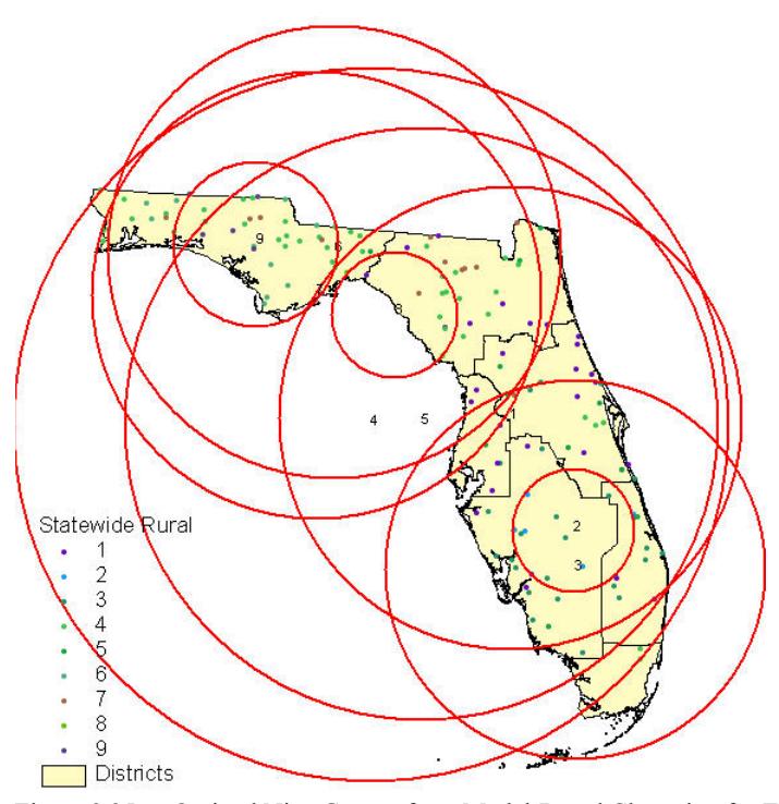
Figure 3.35 Optimal Nine Groups from Model-Based Clustering for TTMSs in Rural Areas
Table 3.9 Number of TTMSs in the Optimal Nine Groups
| Group | Number of TTMSs |
|-------|-----------------|
| 1 | 28 |
| 2 | 5 |
| 3 | 26 |
| 4 | 41 |
| 5 | 13 |
| 6 | 13 |
| 7 | 13 |
| 8 | 2 |
| 9 | 6 |
Figure 3.36 shows the optimal result when the coordinates of the TTMSs are included in the analysis. A more spatially clustered pattern of the TTMSs can be seen. However, as shown in Table 3.10, many groups have only one TTMS.
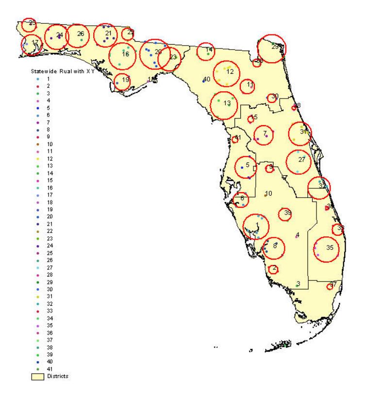
Figure 3.36 Optimal 44 Groups Based on Model-Based Clustering with X-Y for Rural Areas
Table 3.10 Number of TTMSs in the Optimal 44 Groups
| Group | Number of TTMSs |
|-------|-----------------|
| 1 | 6 |
| 2 | 2 |
| 3 | 1 |
| 4 | 1 |
| 5 | 4 |
| 6 | 3 |
| 7 | 4 |
| 8 | 5 |
| 9 | 2 |
| 10 | 1 |
| 11 | 3 |
| 12 | 9 |
| 13 | 5 |
| 14 | 4 |
| 15 | 1 |
| 16 | 2 |
| 17 | 7 |
| 18 | 4 |
| 19 | 1 |
| 20 | 3 |
| 21 | 8 |
| 22 | 7 |
| 23 | 2 |
| 24 | 5 |
| 25 | 6 |
| 26 | 3 |
| 27 | 4 |
| 28 | 5 |
| 29 | 2 |
| 30 | 2 |
| 31 | 2 |
| 32 | 6 |
| 33 | 5 |
| 34 | 3 |
| 35 | 1 |
| 36 | 1 |
| 37 | 3 |
| 38 | 3 |
| 39 | 2 |
| 40 | 3 |
| 41 | 2 |
| 42 | 1 |
| 43 | 1 |
| 44 | 2 |
| | |
### 3.2.2 Refinement of Cluster Results for Rural Areas
The grouping results, shown in Figure 3.35, are examined. Within the same group, the TTMSs in Groups 2, 8, and 9 are similar in their monthly profiles. They are also located in close proximity to each other. Their spatial distributions and MSF profiles are illustrated in Figures 3.37, 3.38, and 3.39, respectively.
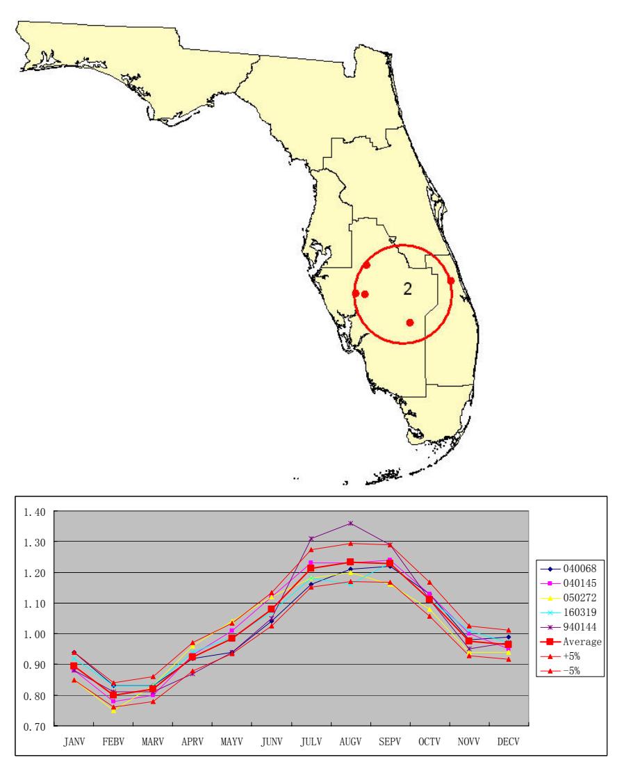
Figure 3.37 Spatial Distribution and Profiles of the TTMSs in Rural Group 2
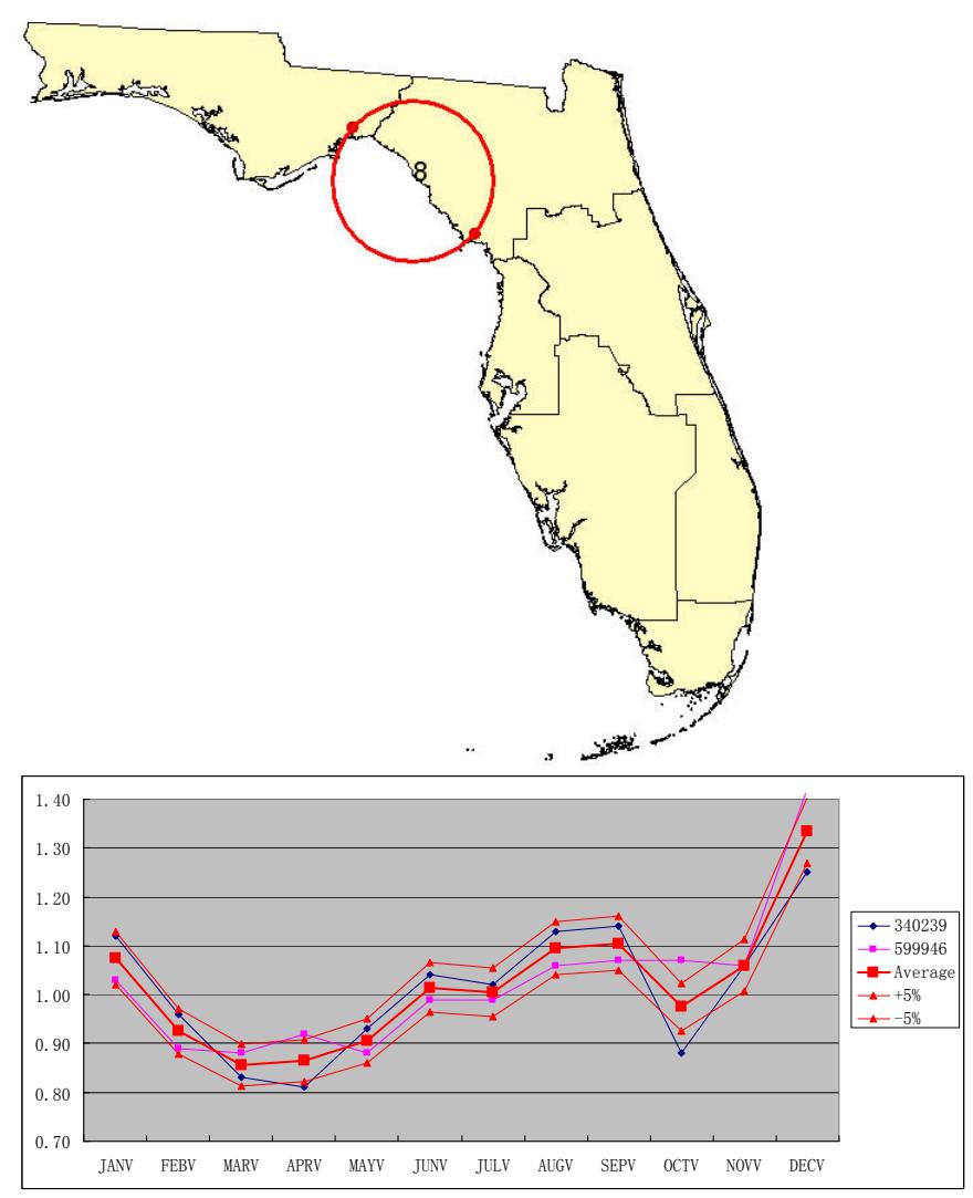
Figure 3.38 Spatial Distribution and Profiles of the TTMSs in Rural Group 8
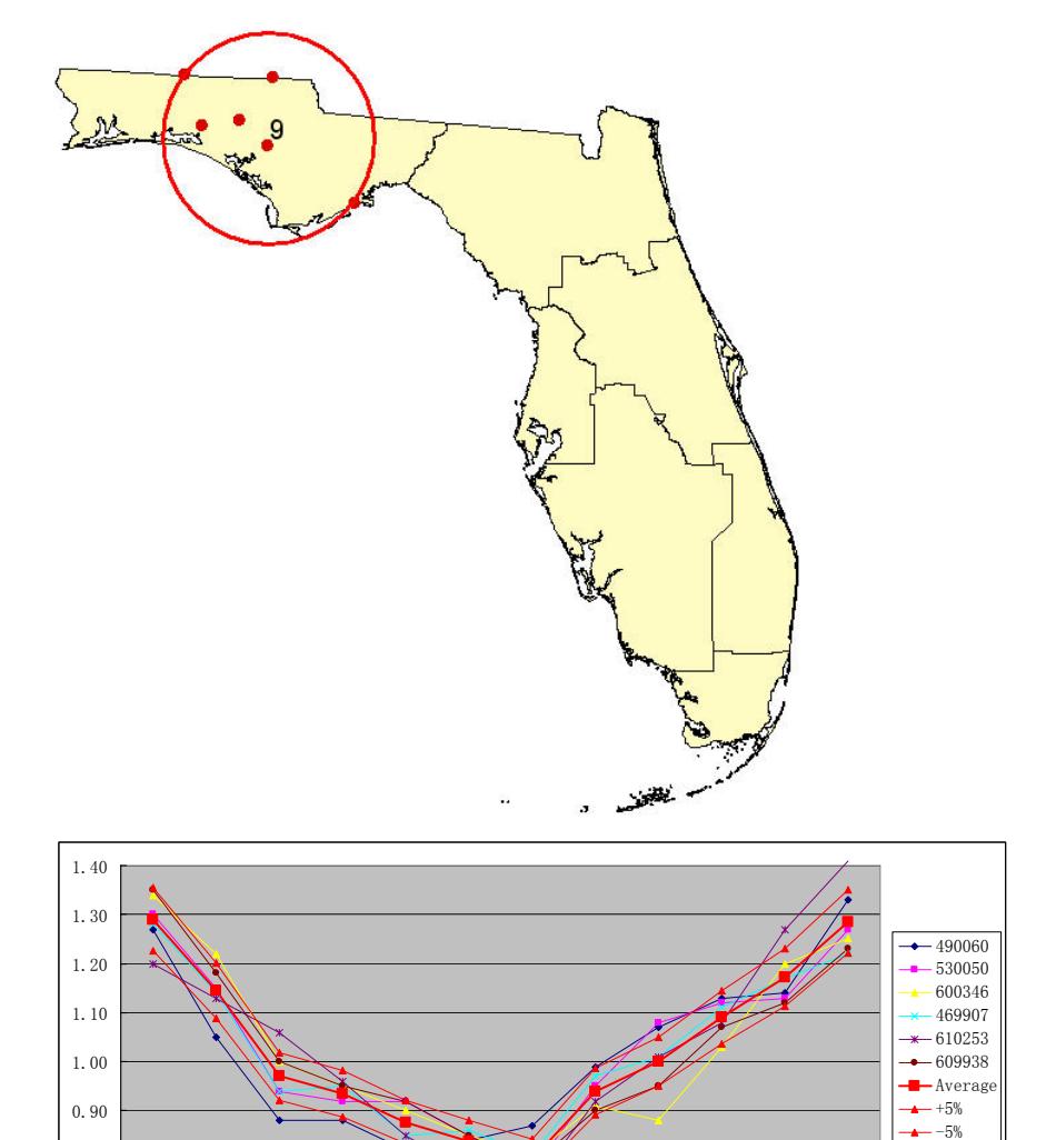
Figure 3.39 Spatial Distribution and Profiles of the TTMSs in Rural Group 9
JANV FEBV MARV APRV MAYV JUNV JULV AUGV SEPV OCTV NOVV DECV
0.70
0.80
For TTMS Groups 1, 3, 4, 5, 6, and 7, the TTMSs in the same groups are located far apart. For example, as shown in Figure 3.40, the TTMSs in Group 1 are from five FDOT districts, which are regrouped into the six new groups shown in Figure 3.41. Figures 3.42 through 3.46 illustrate the profiles for these six new subgroups.
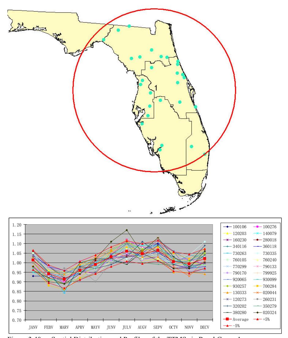
Figure 3.40 Spatial Distribution and Profiles of the TTMSs in Rural Group 1
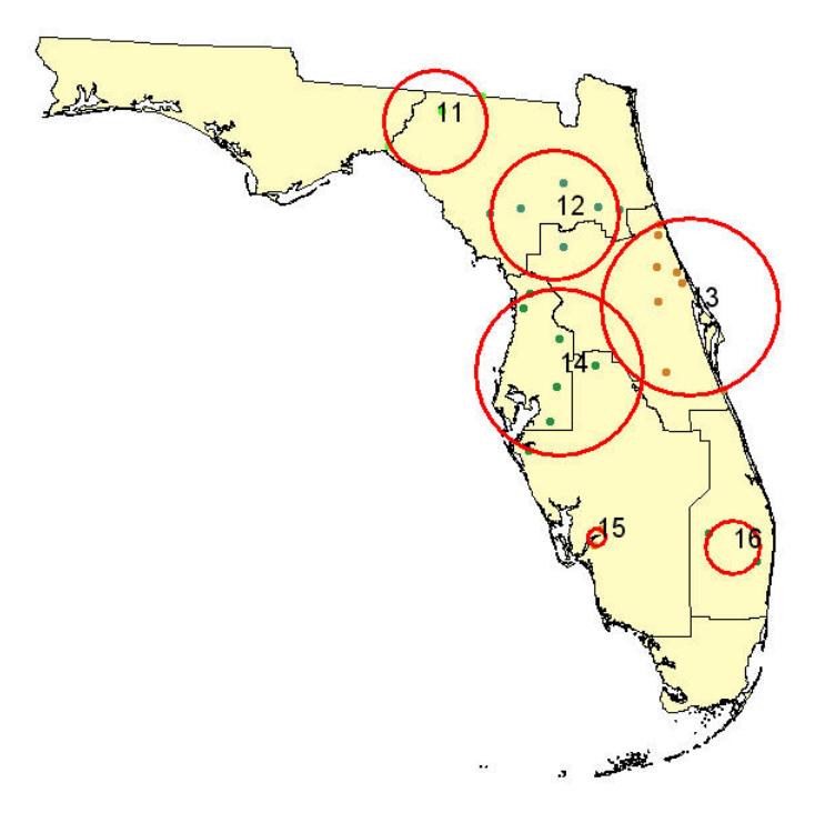
Figure 3.41 New Subgroups Based on Rural Group 1
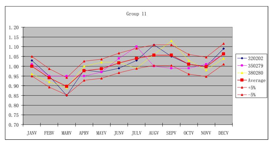
Figure 3.42 Profiles of TTMSs in the New Rural Group 11
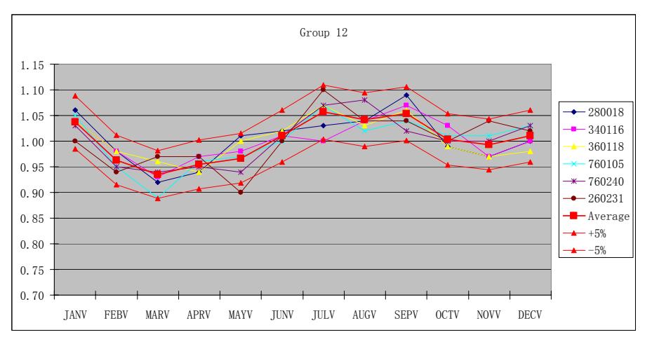
Figure 3.43 Profiles of TTMSs in the New Rural Group 12
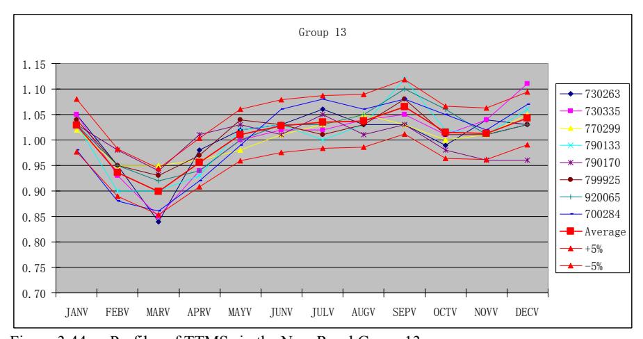
Figure 3.44 Profiles of TTMSs in the New Rural Group 13
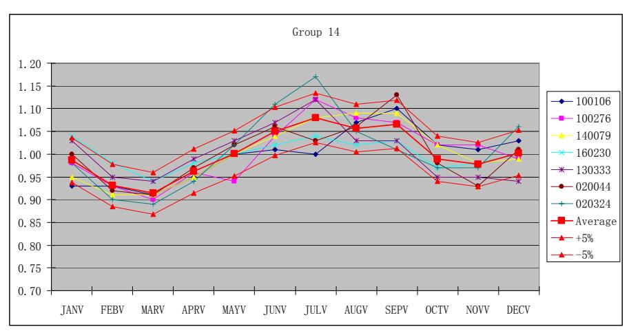
Figure 3.45 Profiles of TTMSs in the New Rural Group 14
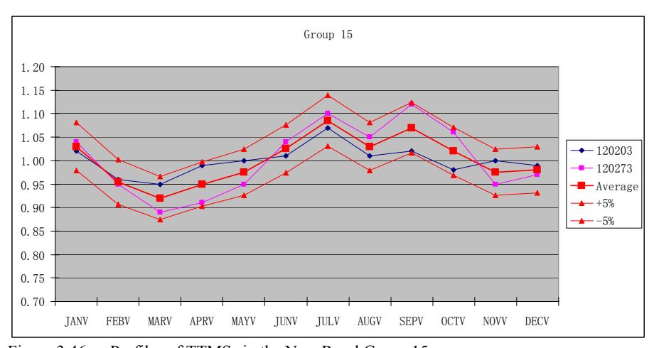
Figure 3.46 Profiles of TTMSs in the New Rural Group 15
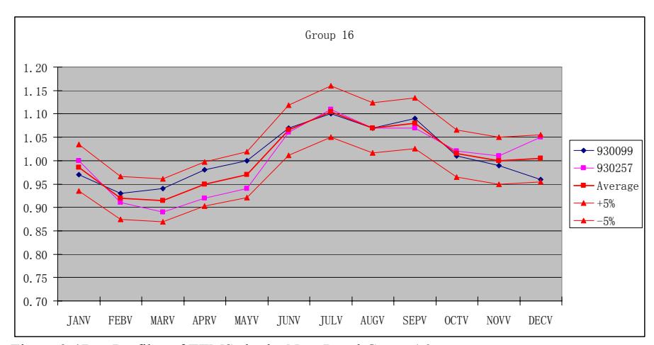
Figure 3.47 Profiles of TTMSs in the New Rural Group 16
Figure 3.48 shows the spatial distributions of TTMSs in Group 3. This group is subdivided into four new subgroups, as shown in Figure 3.49. Figures 3.50 through 3.53 show the profiles for the four new subgroups.
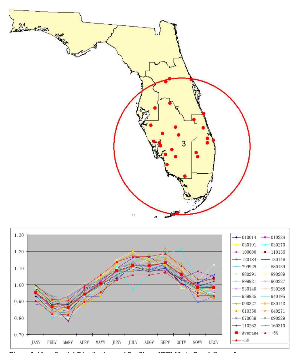
Figure 3.48 Spatial Distribution and Profiles of TTMSs in Rural Group 3
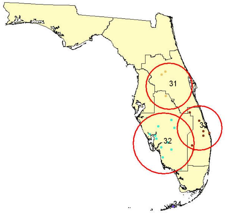
Figure 3.49 Four New Subgroups Created Based on Rural Group 3
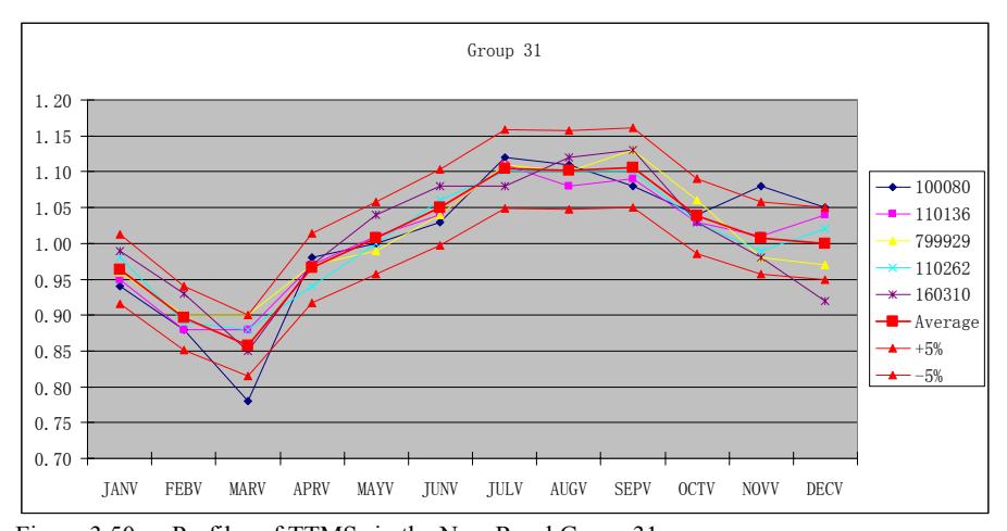
Figure 3.50 Profiles of TTMSs in the New Rural Group 31
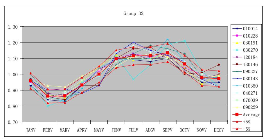
Figure 3.51 Profiles of TTMSs in the New Rural Group 32
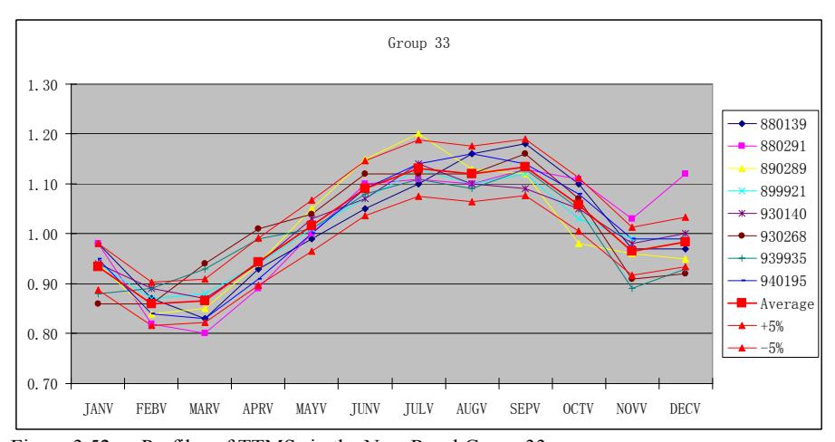
Figure 3.52 Profiles of TTMSs in the New Rural Group 33
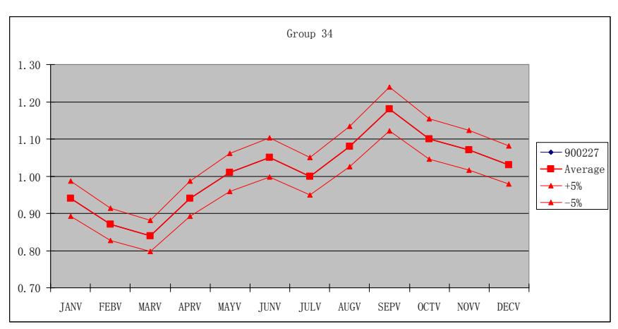
Figure 3.53 Profiles of TTMSs in the New Rural Group 34
The TTMSs in Group 4 are located across the entire state, as indicated in Figure 3.54. These TTMSs are regrouped into four new subgroups, which are shown in Figure 3.55. Figures 3.56 through 3.59 plot the profiles for these four new subgroups.
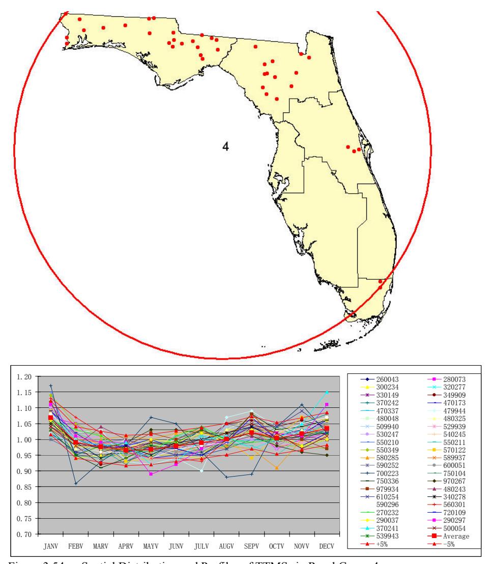
Figure 3.54 Spatial Distribution and Profiles of TTMSs in Rural Group 4
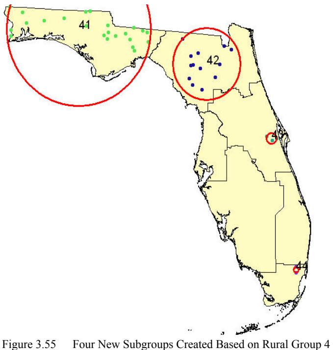
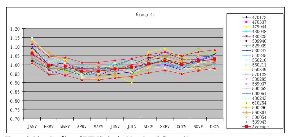
Figure 3.56 Profiles of TTMSs in the New Rural Group 41
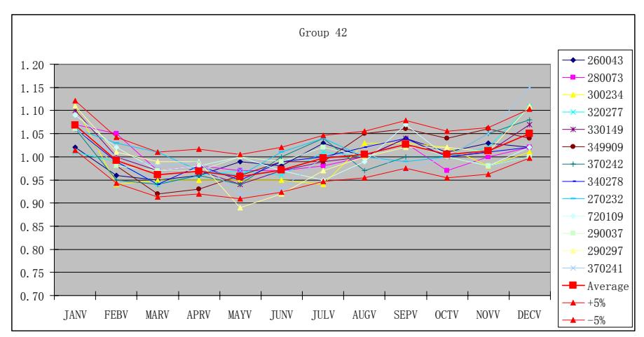
Figure 3.57 Profiles of TTMSs in the New Rural Group 42
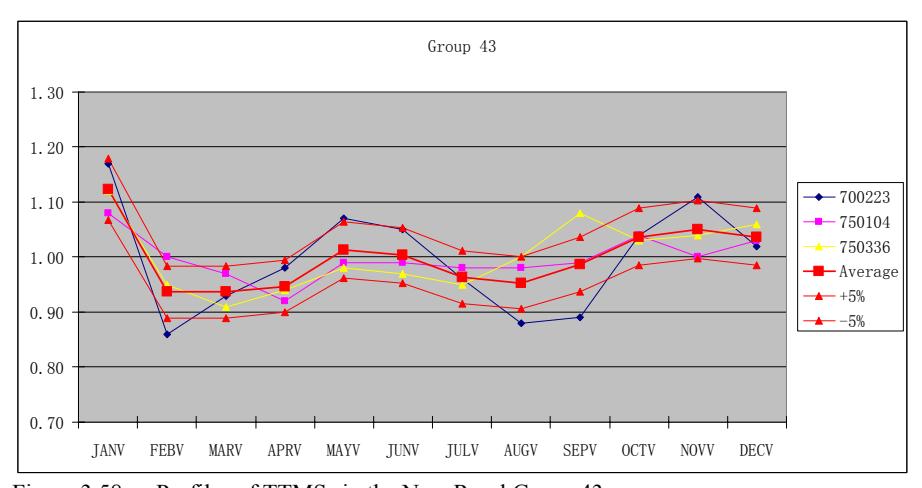
Figure 3.58 Profiles of TTMSs in the New Rural Group 43
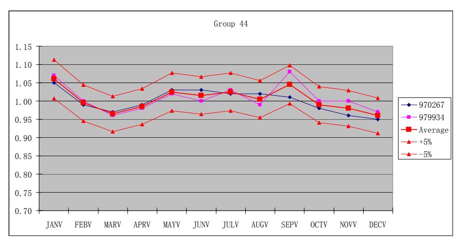
Figure 3.59 Profiles of TTMSs in the New Rural Group 44
Figure 3.60 shows the spatial distribution of the TTMSs in Group 5. Figure 3.61 shows the distributions after four subgroups are created from Group 5. The group profiles for the new subgroups are depicted in Figures 3.62 through 3.65.
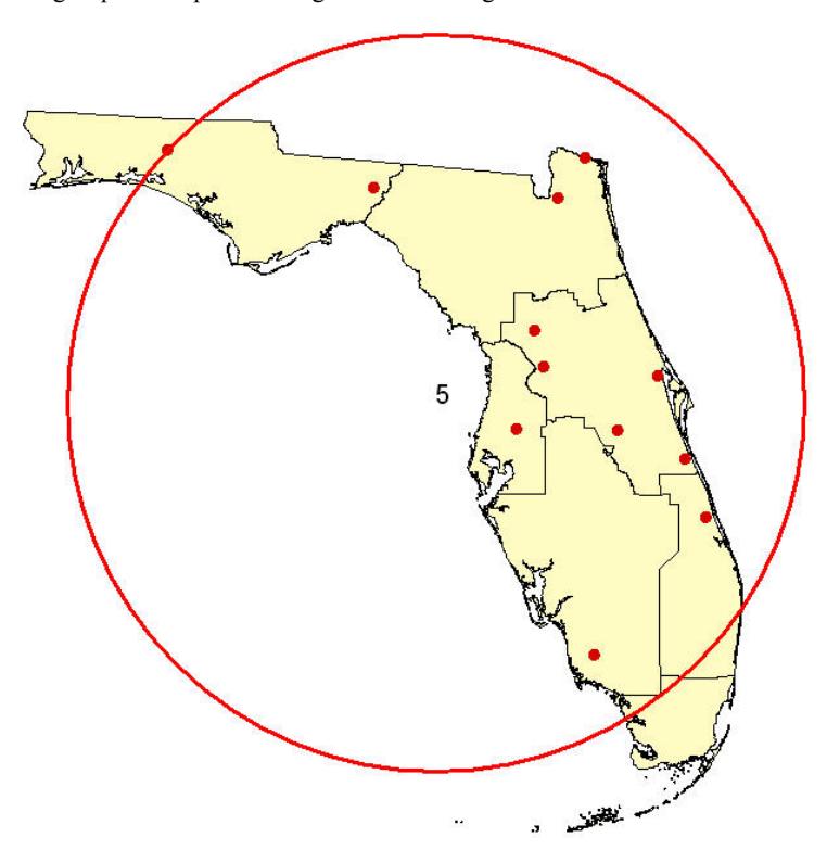
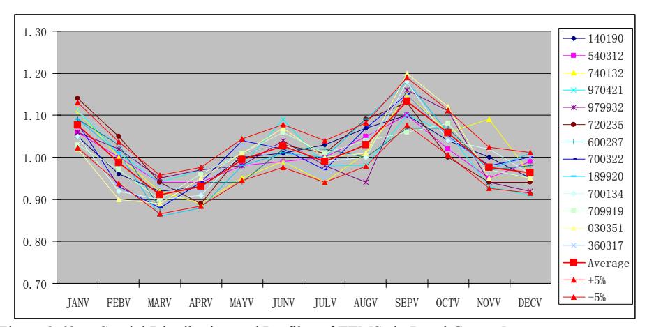
Figure 3.60 Spatial Distribution and Profiles of TTMSs in Rural Group 5
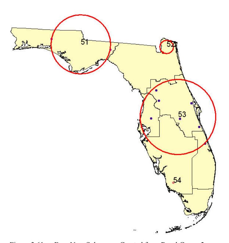
Figure 3.61 Four New Subgroups Created from Rural Group 5
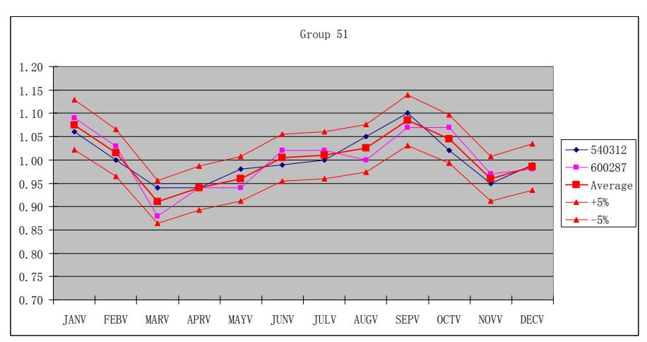
Figure 3.62 Profiles of TTMSs in the New Rural Group 51
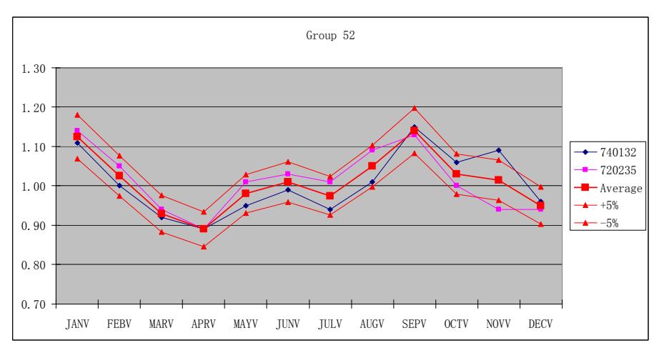
Figure 3.63 Profiles of TTMSs in the New Rural Group 52
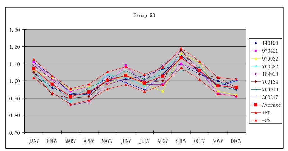
Figure 3.64 Profiles of TTMSs in the New Rural Group 53
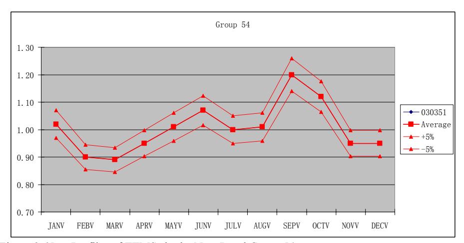
Figure 3.65 Profiles of TTMSs in the New Rural Group 54
The spatial distribution and profiles of the TTMSs in Group 6 are illustrated in Figure 3.66. Note that there are large variations in the MSFs in this group. The TTMSs in this group are divided into four subgroups as shown in Figure 3.67. The group profiles are plotted in Figures 3.68 through 3.71. Also note that the three groups with a single TTMS cannot be combined because they have significantly different patterns.
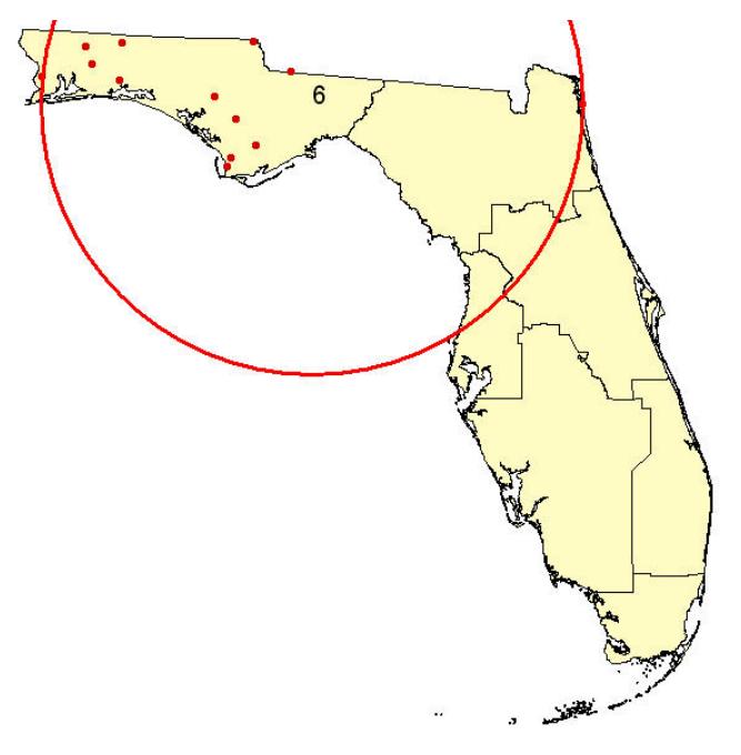
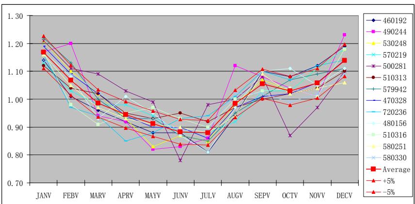
Figure 3.66 Spatial Distribution and Profile of TTMSs in Rural Group 6
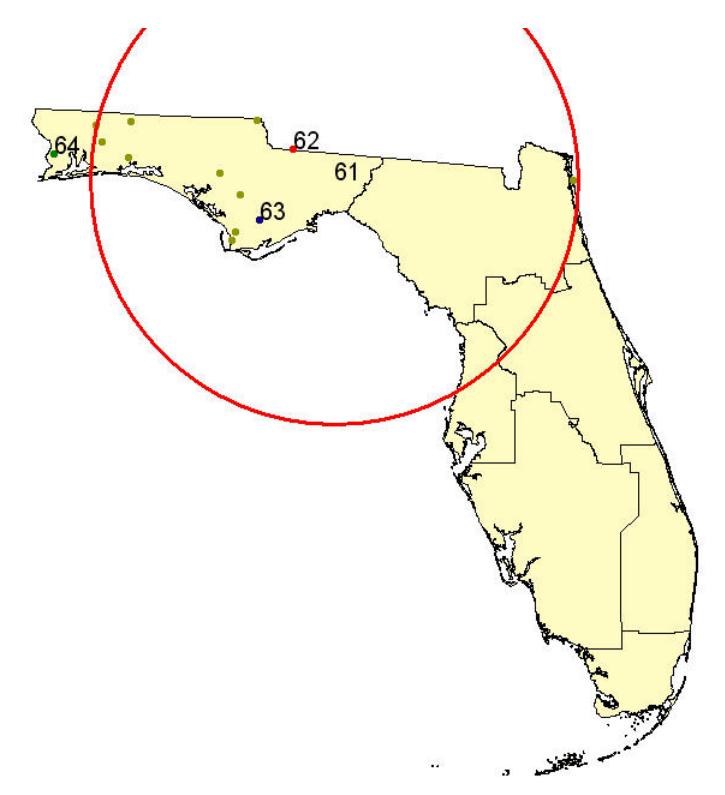
Figure 3.67 Four New Subgroups Created from Rural Group 6
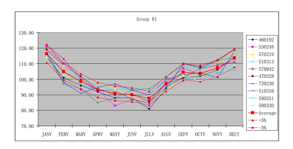
Figure 3.68 Profiles of TTMSs in the New Rural Group 61
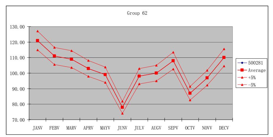
Figure 3.69 Profiles of TTMSs in the New Rural Group 62
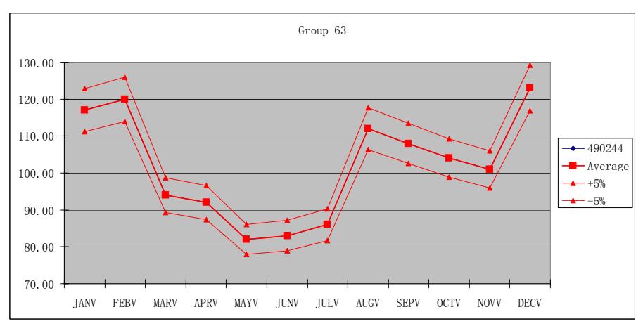
Figure 3.70 Profiles of TTMSs in the New Rural Group 63
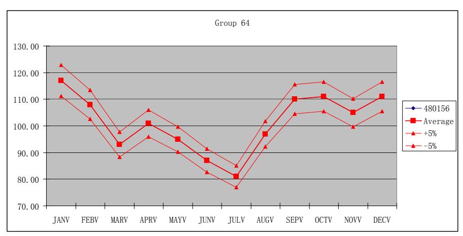
Figure 3.71 Profiles of TTMSs in the New Rural Group 64
Finally, Group 7, as illustrated in Figure 3.72, is split into three new subgroups. These are illustrated in Figure 3.73. The group profiles for the new subgroups are depicted in Figures 3.74 through 3.76.
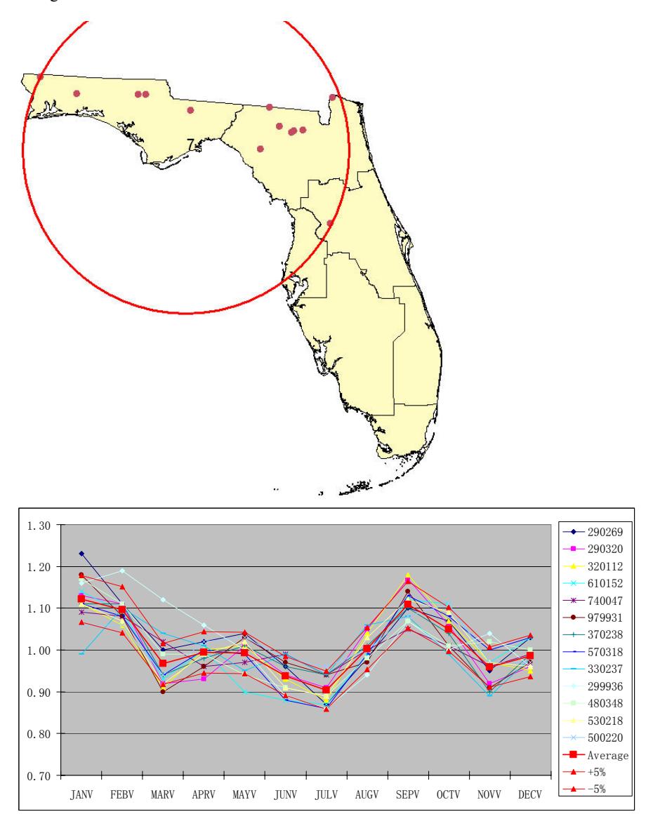
Figure 3.72 Spatial Distribution and Profiles of the TTMSs in Rural Group 7
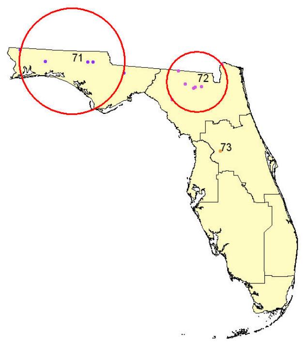
Figure 3.73 Three New Subgroups Created from Rural Group 7
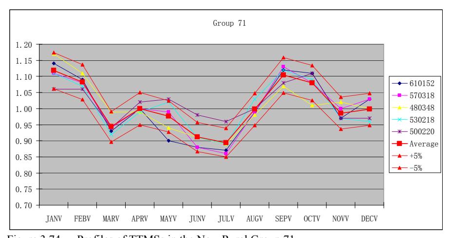
Figure 3.74 Profiles of TTMSs in the New Rural Group 71
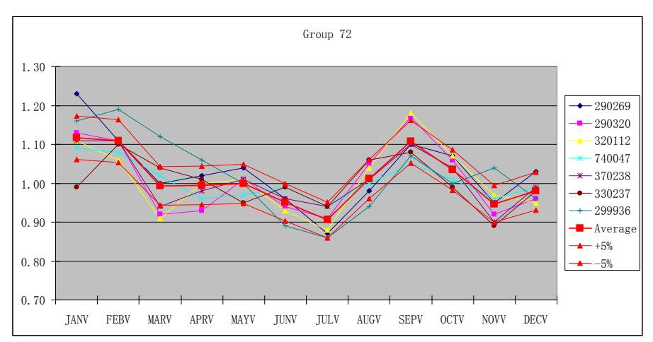
Figure 3.75 Profiles of TTMSs in the New Rural Group 72
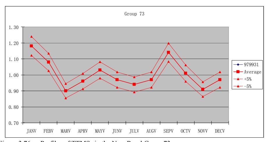
Figure 3.76 Profiles of TTMSs in the New Rural Group 73
After the TTMSs in Groups 1, 3, 4, 5, 6, and 7 are reassigned, a total of 28 TTMS groups are defined for the 147 TTMSs located in rural areas. Figure 3.77 shows the spatial patterns for these 28 TTMS groups. The number of stations allocated to each group is presented in Table 3.9.
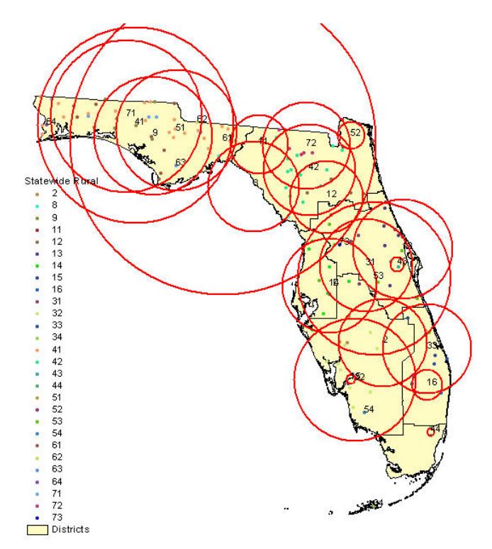
Figure 3.77 Spatial Distribution of Modified TTMS Groups in Rural Areas
Table 3.11 Number of TTMSs in the 28 Rural Groups
| Number of TTMSs |
|-----------------|
| |
| 5 |
| 2 |
| 6 |
| 3 |
| 6 |
| 8 |
| 7 |
| 2 |
| 2 |
| 5 |
| 12 |
| 8 |
| 1 |
| 23 |
| 13 |
| 3 |
| 2 |
| 2 |
| 2 |
| 8 |
| 1 |
| 10 |
| 1 |
| 1 |
| 1 |
| 5 |
| 7 |
| 1 |
| |
# **4. MODELING INFLUENTIAL VARIABLES OF SEASONAL FACTORS IN URBAN AREAS OF FLORIDA**
This chapter describes the regression analyses for identifying variables that potentially influence monthly seasonal factors. The dependent variables are the 12 monthly seasonal factors (MSFs). The regression analyses attempt to establish the relationships between the MSFs and potentially influential variables as linear equations. These equations have the following format:
$$MSF_k = \beta_{0k} + \beta_{1k} x_1 + ... + \beta_{ik} x_i + ... + \beta_{pk} x_p$$
(4-1)
where
*MSFk* = a monthly seasonal factor for month *k,*
β*ik* = the regression coefficient for the *i*th independent variable for month *k*, and
*xi* = the *i*th independent variable.
In this chapter, Section 4.1 describes the data used to compile values of the independent variables and defines the variables used in the analyses. The regression analysis results are described in Sections 4.3, 4.4, and 4.5 for TTMSs in North, Central, and South Florida, respectively.
### **4.1 Definition of Variables for Urban Areas**
Potential independent variables used in regression analysis are those likely to have a causal relationship with seasonal factors. They describe the demographic and socioeconomic characteristics of an area where a TTMS is located. They are selected based on two major considerations: (1) whether the source data are readily available or can be collected easily and economically for both base and forecast years and (2) whether variables can be quantified. The independent variables can be classified generally into the following categories:
- Roadway characteristics,
- Aggregate demographic and socioeconomic variables in the surrounding area of count stations, and
- Geographic spatial location dummy variables from the cluster analysis.
The data used to compile these variables included the following:
- Population and number of occupied hotel/motel rooms at the TAZ level. This population and number are those estimated by county planning departments or metropolitan planning organizations (MPOs) for their 1999 or 2000 transportation models.
- Population, number of retired households by different income groups, number of seasonal households, number of total households, and number of total housing units from the 2000 census at census tract level.
- Employment data for the year 2000 from the InfoUSA database purchased by FDOT. The data include, for each business establishment, the business name, address, location, business type (identified by a SIC code), number of employees, etc.
- Street network with federal functional classification.
The independent variables are described in the following subsections.
### 4.1.1 Roadway Characteristic Variables
Variables in this category are summarized in Table 4.1. The data are from the 2000 FDOT Traffic Information CD and the Roadway Characteristics Inventory (RCI) database. Four variables, *FR*, *PA*, *MA*, and *CO*, are dummy variables that take a value of 0 or 1 and indicate the type of road where a TTMS is located.
Table 4.1 Roadway Characteristic Variables for Urban Roads
| Variable | Description |
|----------|-----------------------------------------------------------------------|
| FR | Equals 0 if TTMS not located on urban freeway; 1 otherwise |
| PA | Equals 0 if TTMS not located on urban principal arterial; 1 otherwise |
| MA | Equals 0 if TTMS not located on urban minor arterial; 1 otherwise |
| CO | Equals 0 if TTMS not located on urban collector; 1 otherwise |
### 4.1.2 Demographic and Socioeconomic Variables
It is well known that socioeconomic conditions affect the travel behavior of trip makers. The variables in this category are designed to reflect the socioeconomic characteristics of the population in the area surrounding a count station. The use of buffer methods is based on the assumption that traffic at a count station is affected by trips generated in or attracted to the area within a certain distance of that count station. Traffic may be made up of local and regional (through) traffic. Buffer methods will not be able to account for the characteristics of all of the traffic generators in the region. This is a limitation of the buffer methods. However, in the absence of more accurate yet simple and practical methods, buffer methods appear to be a reasonable tool for this application.
The variables are compiled using the buffer analysis method. A circular buffer around each count station is created, based on which the variable values are estimated. The buffer radii vary according to the functional classification of the roadway segment where a TTMS is located (Zhao and Chung, 2001). This variation reflects the size of the service area for different types of roads. The buffer radii are five miles for freeway and principal arterials, 0.5 mile for minor arterials, and 0.25 mile for collectors. These radii are based on the common spacing of roads of different function classes. A larger buffer zone implies that the MSFs for a count station are impacted by the characteristics of a larger surrounding area.
### Percentage of student populations by different age groups
Four variables are defined to represent student population groups. They are described in Table 4.2. Their values are computed based on the assumed buffer area for a TTMS. The population of a given age group and the total population in the buffer area are estimated first. The percentage is then computed.
Table 4.2 Student Population Age Group Variables
| Variable | Description | |
|----------|------------------------------------|--|
| ST1 | Population percentage of Age 0-4 | |
| ST2 | Population percentage of Age 5-17 | |
| STU21 | Population percentage of Age 5-10 | |
| STU22 | Population percentage of Age 11-13 | |
| STU23 | Population percentage of Age 14-17 | |
### Percentage of retired households by different income levels
Retired households are defined as households with a retired householder. Retired households are further divided into two subgroups by the state median income level. The percentages of these households out of all retired households are calculated and defined as *Rt\_Low* as *Rt\_High*. The state median income was \$38,500 in 2000. For convenience, the household income levels are divided into \$0 - \$39,999 and \$40,000 and above. The definition of the three retired household related variables is given in Table 4.3.
Table 4.3 Retired Household Variables Based on State-Wide Median Income
| Variable | Description |
|----------|-------------------------------------------------------------------------|
| RETIRE | Percentage of retired households out of total households |
| Rt_Low | Percentage of retired households with low income (\$0 – \$39,999) |
| Rt_High | Percentage of retired households with high income (\$40,000 and above ) |
### Seasonal Household Percentage
Variable *SHP* represents the seasonal households as a percentage of permanent households in a buffer zone around a count station.
### Median Household Income
Variable *MInc* represents the median household income in a buffer zone around a count station.
### Employment Variables
Fourteen variables describing employment in a buffer area surrounding a count station are listed in Table 4.4. InfoUSA employment data are used to compute the values of the variables to reflect the seasonality of economic activities. The InfoUSA database is purchased by FDOT annually and has statewide coverage. For detailed information on each variable and its corresponding SIC codes, please refer to Appendix C.
Table 4.4 Employment Variables for Urban Roads
| Variable | Description | |
|----------|--------------------------------------------------------------------------|--|
| AgriP | Agriculture workers as a percentage of total workers | |
| FishP | Fishing & Hunting workers as a percentage of total workers | |
| TranP | Transportation workers as a percentage of total workers | |
| WholP | Wholesale workers as a percentage of total workers | |
| RtlP | Retail workers as a percentage of total workers | |
| ResaP | Restaurant workers as a percentage of total workers | |
| HotlP | Hotel & Camp workers as a percentage of total workers | |
| EduP | Education workers as a percentage of total workers | |
| RecServP | Amusement & Recreation Services workers as a percentage of | |
| | total workers | |
| MseumP | Museums art galleries & gardens workers as a percentage of total workers | |
| MineP | Mining workers as a percentage of total workers | |
| ManuP | Manufacturing workers as a percentage of total workers | |
| ServP | Services workers as a percentage of total workers | |
| OffP | Office workers as a percentage of total workers | |
| | | |
### 4.1.3 Special Land Use Variables for Urban Models
Variables in this category are designed to account for the effects of special land use types, including universities, tourist attractions, and recreational sites.
### University Variables
Variables in this category are summarized in Table 4.5. *DLEG* is the variable that represents the impact of legislative sessions for the TTMSs located in Leon County. Because community colleges typically operate year round, they may have less seasonal variation in travel related to their activities. The 13 state universities have large enrollments and can potentially affect the seasonality of travel. Two dummy variables, *SU* and *FU,* are created to distinguish mostly residential universities (University of Florida, Florida State University, Florida A&M University, and University of Miami) from universities that have a significant commuting student body. Because Gainesville and Tallahassee are college towns, the universities' impacts are considered to be county wide. For the University of Miami, which is located in a large urban area, the impact area is assumed to be three miles.
Table 4.5 Location Characteristic Variables for Urban Roads
| Variable | Description | |
|----------|------------------------------------------------------------------------------------------------------------|--|
| DLEG | Equals 1 if TTMS is located in Leon County; 0 otherwise | |
| SU | Equals 1 if TTMS is in the county of UF, FSU, and FAMU; or within three miles
of UM or FIT; 0 otherwise | |
| FU | Equals 1 if TTMS is located within three miles of other state universities; 0
otherwise | |
### Tourist Attraction and Recreational Site Variables
The Disney parks and other amusement parks, located in Osceola County, attract a significant number of tourists. These tourists may generate seasonal traffic. Therefore, the variable *DISNEY* is created to represent the tourist effect in Osceola County. The variable assumes a value of 1 if a TTMS is located in Osceola County and 0 otherwise.
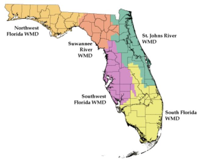
Figure 4.1 Water Management Districts in Florida (Source: Florida Department of Environmental Protection)
In addition to amusement parks, other land uses may also attract visitors, perhaps in larger numbers in some months than others. Such land uses include public beaches, golf courses, marinas, finishing camps, parks, and zoos. They are identified from the land use data that are created by the water management districts in Florida. There are five water management districts in Florida, as shown in Figure 4.1. However, only three have year 2000 land use data, with land use categorized according to the Florida Land Use and Cover Classification System (FLUCCS). Because there are no data from the Suwannee River Water Management District (SRWMD) or the Northwest Florida Water Management District (NWFWMD), the land use variables are only tested in the models for South and Central Florida. Land use is depicted in Figure 4.2.
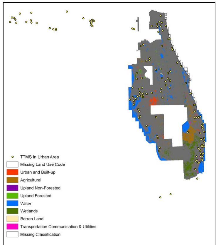
Figure 4.2 Land Use and TTMSs in Urban Areas
Four land use dummy variables are created. The variables and the land use type they represent are summarized in Table 4.6. The values of these variables for a given TTMS are determined based on whether any portion of the buffer area of the TTMS is of one of the four land use types. If a part of the buffer area is of one of the four land uses, the corresponding variable assumes a value of 1. Otherwise, the variable for that TTMS is 0.
Table 4.6 Land Use Dummy Variables for Urban Road
| Variable | FLUCCS Code | Definition | |
|----------|-------------|---------------------------|--|
| LU1 | 1810 | Swimming Beach | |
| LU2 | 1820 | Golf Course | |
| LU3 | 1840 | Marinas and Fishing Camps | |
| LU4 | 1850 | Parks and Zoos | |
### **4.2 Delineation of Model Areas for Urban Areas**
Florida stretches over in the north-south direction over several the climate zones, from temperate in the north to subtropical in the south. South Florida, for example, attracts many visitors and welcomes the return of large numbers of seasonal residents in the winter months because of its warm temperatures. In contrast, summer is the season in North Florida for tourists and for outdoor recreation. Therefore, the same variables may impact traffic in a similar manner, but during different seasons, in North and South Florida. For this reason and for modeling purposes, the state is divided roughly into three regions that represent three climate zones: North Florida, Central Florida, and South Florida. Separate models are developed for each region.
Counties in each region are divided into groups to investigate whether counties within the same region may differ in climate, land use, and demographics. If the counties do differ with regard to these variables, the result may be different seasonal traffic patterns. Regression models are estimated first for one group, then for an expanded group with one more group of counties added. This is repeated until all groups within the same region are included in the models. In this process, model results after each step are carefully examined. This ensures that models do not change significantly in terms of R-squared values, variables included, and coefficients. When such a change is observed, it may indicate that the newly added group of counties may not belong to the region.
As an example, North Florida was originally divided into four groups of counties roughly based on latitude and urban boundaries. Three groups are described in Table 4.7. The fourth group (N3) is Volusia County. Modeling results achieved a higher R-square for both North and Central Florida models by combining the N3 area into the Central Florida region instead of the North Florida region. As a result, Volusia County was removed from the North Florida region and became part of the Central Florida region.
The boundaries of the three regions and the TTMS locations are shown in Figure 4.3. The final models for the three regions are presented in Sections 4.3, 4.4., and 4.5, respectively.
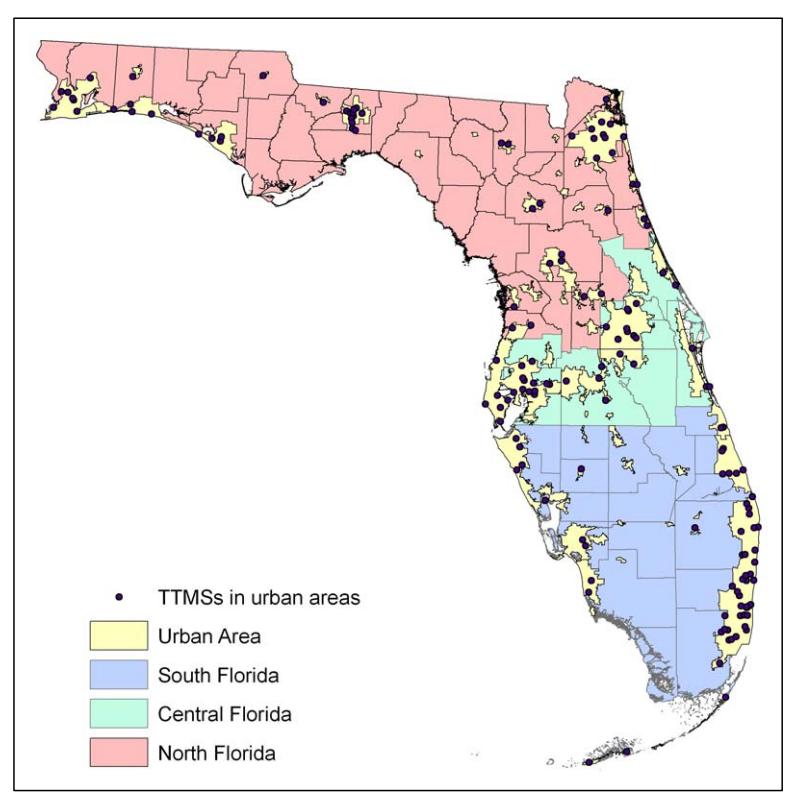
Figure 4.3 Boundaries of Study Areas
The three study areas and the groups of counties within each study area are defined in Tables 4.7, 4.8, and 4.9. These groups of TTMSs in each region are shown in Figures 4.4, 4.5, and 4.6.
Table 4.7 List of Counties within the North Florida Analysis Area
| Area | County | Number of TTMSs | | |
|------|-----------------------------------------------------------------------------------------------------------|-----------------|--|--|
| N1 | Escambia, Santa Rosa, Okaloosa, Walton, Bay, Jackson, Gadsden,
Leon, Columbia, Nassau, Duval, St Johns | 44 | | |
| N2 | Alachua, Putnam, Flagler | 5 | | |
| N4 | Lake, Marion, Citrus, Hernando | 8 | | |
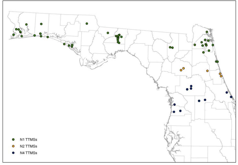
Figure 4.4 TTMSs in Three Urban Study Areas in North Florida
Table 4.8 Study Areas in Central Florida
| Area | County | Number of TTMSs |
|---------|-------------------------------|-----------------|
| N3 | Volusia | 2 |
| C1 (S5) | Pasco, Hillsborough, Pinellas | 18 |
| C2 (S6) | Polk | 4 |
| C3 (S7) | Brevard | 3 |
| C4 (S8) | Orange, Seminole, Osceola | 11 |
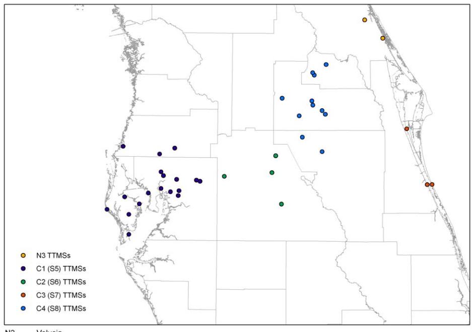
Figure 4.5 TTMSs in Five Urban Study Areas in Central Florida
Table 4.9 List of Counties within the South Florida Analysis Area
| Area | County | Number of TTMSs |
|------|--------------------------------------|-----------------|
| S1 | Broward, Miami-Dade, Palm Beach | 37 |
| S2 | Lee, Collier | 4 |
| S3 | Martin, St Lucie, Indian River | 9 |
| S4 | Charlotte, Sarasota, Manatee, Desoto | 6 |
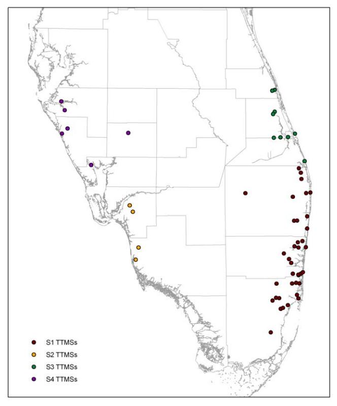
Figure 4.6 TTMSs in Four Urban Study Areas in South Florida
### **4.3 North Florida Model Results**
The regression models of the 12 MSFs for North Florida are given in Table 4.10. A total of 57 TTMSs are included in the model.
Table 4.10 Regression Models for North Florida (NFL)
| h
M
t
on | l
io
Se
Fa
Eq
to
t
as
on
a
c
r
ua
n | 2
R | 2
d
j.
A
R | R
M
S
E |
|-------------------|--------------------------------------------------------------------------------------------------------------------------------------------------------------------------------------------------------------------------------------------------------------------------------------------------------------------------------------------------------------------------------------------------------------------------------------------------------------------------------------------------------------------------------------|------------------------|------------------------|------------------------|
| J
A
N | 0.
9
4
3
8
1.
9
9
4
9
0
2
2
0.
0
0
3
0
1.
1
2
0
0
h
0.
0
1
0
0
4
l
0.
8
4
J
A
N
S
F=
5
S
T
7
S
H
P
5
F
is
P
H
P
+
+
+
+
+
×
×
×
×
t
o
_
0
7
7
M
P
×
se
um | 0.
6
8
1
5 | 0.
6
2
4
6 | 0.
0
1
2
5 |
| F
E
B | 0.
9
9
4
4
9-
0.
0
3
8
8
0.
0
0
2
2
1
0.
6
4
1
2
3
0.
0
0
1
4
F
E
B_
S
F=
5
S
U-
R
E
T
I
R
E
7
7
S
T
5
S
H
P
+
+
×
×
×
×
0.
4
6
8
8
2
M
P
+
×
se
um | 0.
4
5
7
7 | 0.
0
3
4
5 | 0.
0
3
8
6 |
| M
A
R | A
S
1.
0
0
2
0.
0
0
2
6
0
-0
0
0
0
8
3
1
1
S
0.
0
0
0
l
M
R_
F=
7
7-
R
Lo
7
H
P-
5
5
H
P
×
t_
×
×
t
w
o | 0.
2
2
5
7 | 0.
4
9
5
7 | 0.
0
3
2
4 |
| A
P
R | A
S
0.
9
6
4
0
1
0.
0
4
5
4
4
-0
0
2
8
0
8
A
-0
0
0
4
6
3
l
P
R_
F=
F
R
M
H
P
+
×
×
×
t
o | 0.
4
0
8
7 | 0.
3
7
5
2 | 0.
0
3
0
6 |
| M
A
Y | A
S
1.
0
4
1
2
0-
0.
0
2
1
8
3
G
-0
9
2
0
0
3
S
2
3-
0.
0
0
2
3
0
S
0.
8
5
5
6
0
h
M
Y_
F=
L
E
T
H
P-
F
is
P
×
×
×
×
0.
0
0
1
3
0
0.
0
0
5
4
4
l
0.
4
2
0
9
7
0.
0
0
1
9
1
O
f
f
Re
P-
H
P-
M
P
P
+
+
×
t
×
t
×
×
s
o
se
um | 0.
6
9
3
4 | 0.
6
4
2
3 | 0.
0
2
7
4 |
| J
U
N | J
U
N
S
F=
1.
0
8
6
8
4-
2.
0
0
2
5
8
S
T
2
2-
0.
0
0
2
0
7
S
H
P-
1.
0
0
1
3
1
F
is
h
P-
0.
0
0
5
2
2
H
l
P-
×
×
×
×
t
o
_
0.
7
3
8
3
2
M
P
×
se
um | 0.
6
5
0
6 | 0.
6
1
6
3 | 0.
0
3
8
3 |
| J
U
L | J
U
L_
S
F=
1.
0
0
8
2
7
0.
0
5
1
5
3
S
U
0.
0
0
3
2
2
R
Lo
-1
6
5
6
8
4
S
T
2
2-
0.
0
0
2
2
6
S
H
P-
+
+
t_
×
×
×
×
w
0.
0
0
9
1
1
H
l
P
0.
0
0
1
3
4
E
d
P-
0.
6
7
1
3
1
M
P
+
×
t
×
×
o
se
um | 0.
6
2
6
9 | 0.
5
7
3
6 | 0.
0
5
4
8 |
| A
G
U | A
U
G
S
F=
0.
9
7
4
4
5
0.
0
1
6
1
2
L
E
G
0.
0
0
2
7
5
R
Lo
-0
4
7
6
8
4
S
T
1-
0.
0
0
0
7
3
5
7
1
S
H
P
+
+
t_
×
×
×
×
w
_
0.
0
0
3
2
7
W
ho
l
P
0.
0
0
1
6
1
Rc
Se
P-
0.
2
7
2
0
3
M
P
+
+
×
×
×
rv
se
um | 0.
7
7
7
6 | 0.
7
4
5
8 | 0.
0
1
8
0 |
| S
E
P | S
E
P_
S
F=
1.
0
1
2
9
0-
0.
0
3
2
8
5
S
U
0.
0
0
1
5
0
R
E
T
I
R
E
+
×
× | 0.
2
8
7
9 | 0.
2
6
1
5 | 0.
0
4
4
5 |
| O
C
T | O
C
T_
S
F=
0.
9
6
6
9
2-
0.
0
2
7
1
6
S
U
0.
8
5
1
5
3
S
T
2
3
0.
0
0
2
0
1
S
H
P
0.
0
0
7
8
1
H
l
P-
+
+
+
t
×
×
×
×
o
0.
0
0
1
0
8
E
d
P
× | 0.
5
7
7
6 | 0.
5
3
6
2 | 0.
0
3
6
5 |
| N
O
V | N
O
V_
S
F=
1.
0
0
2
1
2
0.
0
0
2
7
6
S
H
P
0.
0
0
9
1
6
H
l
P
1.
0
0
1
4
4
M
P
+
+
+
×
×
t
×
o
se
um | 0.
6
0
2
0 | 0.
5
7
9
5 | 0.
0
5
9
1 |
| D
E
C | l
D
E
C_
S
F=
0.
9
9
2
8
0
0.
0
0
3
4
8
S
H
P
0.
0
0
5
4
4
Tr
P
0.
0
1
6
4
8
H
P
1.
3
7
4
0
2
M
P
+
+
+
+
×
×
×
t
×
an
o
se
um | 0.
6
1
6
4 | 0.
5
8
6
9 | 0.
0
8
5
1 |
The variables included in the above models are listed in Table 4.11, along with their partial R2 values and the months for which they are significant. Table 4.12 and 4.13 list only those variables that have a partial R2 greater than 0.05. Table 4.12 lists the variables by name, while Table 4.13 lists them by partial R2 value.
The models show that *SHP* (percentage of seasonal households), *MseumP* (percentage of museums/art/galleries/gardens workers), and *HotlP* (percentage of hotel & camp workers) appear in most of the models with relatively large partial R2 values. *Rt\_Low* (percentage of retired households with low income), *RETIRE* (percentage of retired households), *FR* (freeway), *ST22* (percentage of population ages 11-13), and *ST23* (percentage of population ages 14-17) are some of the variables that appear infrequently. However, these variables have noticeable partial R2 values when they do appear in the models.
In general, variables representing tourist related activities, such as fishing, museum, and hotel related employment, tend to have a positive coefficient in the winter months and a negative sign in the summer months. This suggests that the tourist season is summer in North Florida.
The variable that represents residential universities, *SU*, appears in the February, September, and October models with a negative coefficient. In contrast, it appears in the July model with a positive coefficient. This is possibly due to an increase in traffic related to the beginning of the academic year and a decrease in traffic caused by holidays during summer.
Variable *SHP* appears in all models except for April and September. Note that there is a positive coefficient during the colder months (from October to February) and a negative coefficient during the warm months (March, and May to August). This shows that there may be more seasonal households in North Florida during the warm months than the cold months.
Variables representing the student population ages 11-17 (*ST22* and *ST23*) tend to be associated with more traffic during the summer vacation season (May, June, and July) but less traffic during January and February.
The variable that represents low income retired households, *Rt\_Low*, is included in the March model with a negative coefficient and the August model with a positive coefficient. Similarly, the variable *RETIRE* appears with a negative coefficient in the February model while a positive coefficient in the October model. This suggests that low-income retired households tend to have greater activity during February and March than August and September.
Table 4.11 Variables from Model NFL Sorted by Month and Partial R2 Value
| | Variable Partial R2 | Month |
|--------|---------------------|-------|
| SHP | 0.2964 | JAN |
| MseumP | 0.1659 | JAN |
| ST22 | 0.0775 | JAN |
| HotlP | 0.0709 | JAN |
| FishP | 0.0473 | JAN |
| MseumP | 0.1572 | FEB |
| RETIRE | 0.144 | FEB |
| SU | 0.1046 | FEB |
| SHP | 0.0851 | FEB |
| ST23 | 0.0569 | FEB |
| Rt_Low | 0.3359 | MAR |
| HotlP | 0.1367 | MAR |
| SHP | 0.0501 | MAR |
| FR | 0.1973 | APR |
| HotlP | 0.1291 | APR |
| MA | 0.0822 | APR |
| SHP | 0.2662 | MAY |
| ST23 | 0.1439 | MAY |
| MseumP | 0.0745 | MAY |
| | | |
| Variable | Partial R2 | Month |
|----------|------------|-------|
| HotlP | 0.0395 | MAY |
| RestP | 0.0407 | MAY |
| FishP | 0.0368 | MAY |
| OffP | 0.0617 | MAY |
| LEG | 0.0301 | MAY |
| MseumP | 0.2701 | JUN |
| SHP | 0.1298 | JUN |
| ST22 | 0.1487 | JUN |
| FishP | 0.0642 | JUN |
| HotlP | 0.0377 | JUN |
| MseumP | 0.1851 | JUL |
| SHP | 0.1178 | JUL |
| ST22 | 0.1102 | JUL |
| Rt_Low | 0.073 | JUL |
| SU | 0.0678 | JUL |
| HotlP | 0.0404 | JUL |
| EdP | 0.0325 | JUL |
| Rt_Low | 0.3854 | AUG |
| MseumP | 0.1438 | AUG |
| | | |
| | Variable Partial R2 | Month |
|---------|---------------------|-------|
| SHP | 0.0619 | AUG |
| RcServP | 0.0647 | AUG |
| WholP | 0.0344 | AUG |
| ST1 | 0.0603 | AUG |
| LEG | 0.0271 | AUG |
| RETIRE | 0.2256 | SEP |
| SU | 0.0623 | SEP |
| SHP | 0.3353 | OCT |
| HotlP | 0.0767 | OCT |
| SU | 0.0673 | OCT |
| ST23 | 0.046 | OCT |
| EdP | 0.0522 | OCT |
| MseumP | 0.3448 | NOV |
| SHP | 0.2035 | NOV |
| HotlP | 0.0537 | NOV |
| MseumP | 0.2973 | DEC |
| SHP | 0.1648 | DEC |
| HotlP | 0.0742 | DEC |
| TranP | 0.08 | DEC |
| | | |
Table 4.12 Variables from Model NFL Sorted by Name and Partial R2 Value
| | Variable Partial R2 | Month |
|--------|---------------------|-------|
| EdP | 0.0522 | OCT |
| FishP | 0.0642 | JUN |
| FR | 0.1973 | APR |
| HotlP | 0.1367 | MAR |
| HotlP | 0.1291 | APR |
| HotlP | 0.0767 | OCT |
| HotlP | 0.0742 | DEC |
| HotlP | 0.0709 | JAN |
| HotlP | 0.0537 | NOV |
| MA | 0.0822 | APR |
| MseumP | 0.3448 | NOV |
| MseumP | 0.2973 | DEC |
| MseumP | 0.2701 | JUN |
| MseumP | 0.1851 | JUL |
| MseumP | 0.1659 | JAN |
| MseumP | 0.1572 | FEB |
| Variable | Partial R2 | Month |
|----------|------------|-------|
| MseumP | 0.1438 | AUG |
| MseumP | 0.0745 | MAY |
| OffP | 0.0617 | MAY |
| RcServP | 0.0647 | AUG |
| RETIRE | 0.2256 | SEP |
| RETIRE | 0.144 | FEB |
| SHP | 0.3353 | OCT |
| SHP | 0.2964 | JAN |
| SHP | 0.2662 | MAY |
| SHP | 0.2035 | NOV |
| SHP | 0.1648 | DEC |
| SHP | 0.1298 | JUN |
| SHP | 0.1178 | JUL |
| SHP | 0.0851 | FEB |
| SHP | 0.0619 | AUG |
| SHP | 0.0501 | MAR |
| | | |
| Value | | | |
|--------|---------------------|-------|--|
| | Variable Partial R2 | Month | |
| ST1 | 0.0603 | AUG | |
| ST22 | 0.1487 | JUN | |
| ST22 | 0.1102 | JUL | |
| ST22 | 0.0775 | JAN | |
| ST23 | 0.1439 | MAY | |
| ST23 | 0.0569 | FEB | |
| Rt_Low | 0.3854 | AUG | |
| Rt_Low | 0.3359 | MAR | |
| Rt_Low | 0.073 | JUL | |
| SU | 0.1046 | FEB | |
| SU | 0.0678 | JUL | |
| SU | 0.0673 | OCT | |
| SU | 0.0623 | SEP | |
| TranP | 0.08 | DEC | |
| WholP | 0.0344 | AUG | |
Table 4.13 Variables from Model NFL Sorted by Partial R2 Value
| Partial R2 Month | |
|------------------|-----|
| 0.3854 | AUG |
| 0.3448 | NOV |
| 0.3359 | MAR |
| 0.3353 | OCT |
| 0.2973 | DEC |
| 0.2964 | JAN |
| 0.2701 | JUN |
| 0.2662 | MAY |
| 0.2256 | SEP |
| 0.2035 | NOV |
| 0.1973 | APR |
| 0.1851 | JUL |
| 0.1659 | JAN |
| 0.1648 | DEC |
| 0.1572 | FEB |
| 0.1487 | JUN |
| | |
| Variable | Partial R2 Month | |
|----------|------------------|-----|
| RETIRE | 0.144 | FEB |
| ST23 | 0.1439 | MAY |
| MseumP | 0.1438 | AUG |
| HotlP | 0.1367 | MAR |
| SHP | 0.1298 | JUN |
| HotlP | 0.1291 | APR |
| SHP | 0.1178 | JUL |
| ST22 | 0.1102 | JUL |
| SU | 0.1046 | FEB |
| SHP | 0.0851 | FEB |
| MA | 0.0822 | APR |
| TranP | 0.08 | DEC |
| ST22 | 0.0775 | JAN |
| HotlP | 0.0767 | OCT |
| MseumP | 0.0745 | MAY |
| HotlP | 0.0742 | DEC |
| Variable | Partial R2 Month | |
|----------|------------------|-----|
| Rt_Low | 0.073 | JUL |
| HotlP | 0.0709 | JAN |
| SU | 0.0678 | JUL |
| SU | 0.0673 | OCT |
| RcServP | 0.0647 | AUG |
| FishP | 0.0642 | JUN |
| SU | 0.0623 | SEP |
| SHP | 0.0619 | AUG |
| OffP | 0.0617 | MAY |
| ST1 | 0.0603 | AUG |
| ST23 | 0.0569 | FEB |
| HotlP | 0.0537 | NOV |
| EdP | 0.0522 | OCT |
| SHP | 0.0501 | MAR |
| | | |
### **4.4 Central Florida Model Results**
The regression models of the MSFs in Central Florida (CFL) are given in Table 4.14. A total of 38 TTMSs are included in the model.
Table 4.14 Regression Models for Central Florida (CFL)
| h
M
t
on | l
io
Se
Fa
Eq
to
t
as
on
a
c
r
ua
n | 2
R | 2
d
j.
A
R | R
M
S
E |
|-------------------|---------------------------------------------------------------------------------------------------------------------------------------------------------------------------------------------------------------------------------------------------------------------------------------------------------------------------------------------------------------------------------------------------------|------------------------|------------------------|------------------------|
| J
A
N | J
A
N
S
F=
1.
0
5
2
9
6
0.
0
4
3
5
4
L
U
2
0.
0
8
5
2
8
L
U
3-
0.
0
0
2
5
3
R
Lo
+
+
×
×
×
t_
w
_ | 0.
4
9
6
6 | 0.
4
5
2
2 | 0.
0
3
8
6 |
| F
E
B | 0.
9
9
2
2
0-
0.
0
0
1
9
2
F
E
B_
S
F=
R
E
T
I
R
E
× | 0.
3
2
6
6 | 0.
3
0
9
7 | 0.
0
3
2
9 |
| M
A
R | A
S
0.
9
4
0.
0
4
1
8
9
A
-0
0
0
1
9
S
0.
0
3
8
0
A
0.
0
0
1
0
6
l
M
R_
F=
5
5
5
P
7
H
P-
7
i
P-
R
P
+
×
×
×
×
t
g
r | 0.
9
2
3
5 | 0.
4
2
9
5 | 0.
0
3
2
8 |
| A
P
R | A
S
0.
9
6
1
9
3-
0.
0
3
7
5
2
P
R_
F=
M
in
P
×
e | 0.
1
1
3
0 | 0.
0
8
8
4 | 0.
0
2
5
8 |
| M
A
Y | A
S
1.
0
4
6
9
6
0.
0
5
2
5
2
C
O
-9
3
5
2
5
3
E-
7
0.
0
0
0
5
2
9
3
6
Se
M
Y_
F=
M
In
P
+
×
×
×
c-
rv | 0.
3
6
7
0 | 0.
3
1
1
1 | 0.
0
2
0
2 |
| J
U
N | J
U
N
S
F=
0.
9
8
3
7
0
0.
0
0
1
3
0
R
E
T
I
R
E
0.
0
5
0
3
9
A
i
P
+
+
×
×
g
r
_ | 0.
5
4
8
1 | 0.
5
2
2
3 | 0.
0
2
3
0 |
| J
U
L | J
U
L_
S
F=
1.
1
4
2
5
7-
0.
0
8
9
0
4
D
I
S
N
-0
0
5
9
6
3
L
U
4-
0.
0
0
0
0
0
2
0
3
M
In
×
×
×
c | 0.
3
3
7
7 | 0.
2
7
9
3 | 0.
0
4
7
0 |
| A
U
G | A
U
G
S
F=
1.
0
3
8
1
2-
0.
0
2
2
9
8
P
A
-0
0
6
8
1
0
D
I
S
N
-0
0
3
7
9
0
L
U
2
0.
0
0
1
1
1
S
H
P
+
×
×
×
×
_
0.
0
9
4
2
8
A
i
P-
0.
0
2
3
2
9
O
f
f
P
+
×
×
g
r | 0.
7
6
7
1 | 0.
7
2
2
0 | 0.
0
2
9
2 |
| S
E
P | S
E
P_
S
F=
1.
1
4
0
0
4-
0.
0
4
8
0
9
P
A
-1
5
9
2
6
1
S
T
2
2
0.
0
6
0
4
8
A
i
P
+
×
×
×
g
r | 0.
5
3
5
7 | 0.
4
9
4
7 | 0.
0
3
3
5 |
| O
C
T | h-
O
C
T_
S
F=
1.
0
4
0
1
3-
0.
0
9
0
1
7
C
O
0.
0
0
3
2
6
R
H
ig
1.
0
5
5
5
1
S
T
2
3
0.
0
4
1
5
2
A
i
P
+
+
×
×
t_
×
×
g
r | 0.
5
6
0
0 | 0.
5
0
6
6 | 0.
0
2
2
9 |
| N
O
V | 1.
0
1
2
0.
0
6
1
0
1
0.
0
0
4
0
9
0.
0
0
3
0
8
d
N
O
V_
S
F=
7
7
M
A
Tr
P-
E
P
+
+
×
×
×
an | 0.
4
1
8
9 | 0.
3
6
6
7 | 0.
0
2
1
5 |
| D
E
C | C_
S
1.
0
0
8
6
1
0.
0
8
6
3
9
A
D
E
F=
M
+
× | 0.
1
3
3
6 | 0.
1
0
9
6 | 0.
0
0
5
5 |
For the Central Florida models, significant variables are *AgriP* (percentage of agriculture employment) and *RETIRE* (percentage of retired households). *AgriP* appears most often and contributes a large portion of partial R2 to the June, August, September, and October models with a positive sign.
Of the variables that describe tourist attractions and recreational sites, *LU2* (the golf course variable) and *LU3* (the marinas/fishing camp variable) are included in the January model with a positive coefficient, indicating a decreased level of travel related to these activities. *LU4* (the parks and zoos variable) is selected by the July model with a negative sign, pointing to an increase in travel to parks and zoos. The variable *DISNEY* shows up in models for July and August with a negative sign. This means traffic around Disney parks tends to increase during these two months, which coincide with school summer vacation time.
Roadway characteristic variables (*PA*, *MA*, and *CO*) are selected by two models. *PA* (principal arterial) enters the March model with a positive coefficient and the September model with a negative coefficient. This suggests that principal arterials tend to have more traffic in September but lower traffic in March in rural areas. The *MA* (minor arterial) variable is selected by the November and December models. Their coefficients are both positive, suggesting that minor arterials carry less traffic during the last two months of a year. *CO* (collector) appears in the May model with a positive coefficient and in the October model with a negative coefficient. This indicates that traffic on collectors tends to increase during October and decrease during May. The model results also show that retired households seem to contribute to the increase in traffic during February and the decrease during June. *MInc* (median household income) appears in the May and July models with a negative sign. This suggests that, during these two months in Central Florida, the higher the median income is, the more traffic is generated.
Table 4.15 lists all of the variables included in the above models, along with their partial R2 values and the months for which they significant. Table 4.16 and 4.17 list all of the variables that have a partial R2 larger than 0.05. Table 4.16 sorts the variables by name, while Table 4.17 sorts them by partial R2 value.
Table 4.15 Variables from Model CFL Sorted by Month and Partial R2 Value
| | Variable Partial R2 | Month |
|--------|---------------------|-------|
| Rt_Low | 0.2177 | JAN |
| LU3 | 0.1914 | JAN |
| LU2 | 0.0875 | JAN |
| RETIRE | 0.3266 | FEB |
| SHP | 0.2821 | MAR |
| PA | 0.1863 | MAR |
| AgriP | 0.0639 | MAR |
| RtlP | 0.0601 | MAR |
| MineP | 0.113 | APR |
| CO | 0.1625 | MAY |
| MInc | 0.1198 | MAY |
| ServP | 0.0846 | MAY |
| | | |
| Variable | Partial R2 | Month |
|----------|------------|-------|
| AgriP | 0.3462 | JUN |
| RETIRE | 0.2019 | JUN |
| MInc | 0.1334 | JUL |
| DISN | 0.1193 | JUL |
| LU4 | 0.0851 | JUL |
| AgriP | 0.4459 | AUG |
| SHP | 0.1321 | AUG |
| DISN | 0.0584 | AUG |
| OffP | 0.0572 | AUG |
| LU2 | 0.0367 | AUG |
| PA | 0.0369 | AUG |
| PA | 0.2403 | SEP |
| | | |
| | Variable Partial R2 | Month |
|---------|---------------------|-------|
| ST22 | 0.1238 | SEP |
| AgriP | 0.1716 | SEP |
| ST23 | 0.1912 | OCT |
| AgriP | 0.1494 | OCT |
| Rt_High | 0.0832 | OCT |
| CO | 0.1363 | OCT |
| MA | 0.1797 | NOV |
| EdP | 0.1144 | NOV |
| TranP | 0.1248 | NOV |
| MA | 0.1336 | DEC |
| | | |
| Variables from Model CFL Sorted by Name and Partial R2
Table 4.16
Value |
|-------------------------------------------------------------------------------|
|-------------------------------------------------------------------------------|
| Month
NOV
JAN |
|---------------------|
| |
| |
| |
| OCT |
| OCT |
| SEP |
| MAR |
| AUG |
| MAY |
| MAR |
| FEB |
| JUN |
| SEP |
| |
| Variable | Partial R2 | Month |
|----------|------------|-------|
| PA | 0.1863 | MAR |
| OffP | 0.0572 | AUG |
| MineP | 0.113 | APR |
| MInc | 0.1334 | JUL |
| MInc | 0.1198 | MAY |
| MA | 0.1797 | NOV |
| MA | 0.1336 | DEC |
| LU4 | 0.0851 | JUL |
| LU3 | 0.1914 | JAN |
| LU2 | 0.0875 | JAN |
| EdP | 0.1144 | NOV |
| DISN | 0.1193 | JUL |
| | | |
| | Variable Partial R2 | Month |
|--------|---------------------|-------|
| DISN | 0.0584 | AUG |
| CO | 0.1625 | MAY |
| CO | 0.1363 | OCT |
| AgriP | 0.4459 | AUG |
| AgriP | 0.3462 | JUN |
| AgriP | 0.1716 | SEP |
| AgriP | 0.1494 | OCT |
| AgriP | 0.0639 | MAR |
| TranP | 0.1248 | NOV |
| Rt_Low | 0.2177 | JAN |
| | | |
Table 4.17 Variables from Model CFL Sorted by Partial R2 Value
| | Variable Partial R2 | Month |
|--------|---------------------|-------|
| AgriP | 0.4459 | AUG |
| AgriP | 0.3462 | JUN |
| RETIRE | 0.3266 | FEB |
| SHP | 0.2821 | MAR |
| PA | 0.2403 | SEP |
| Rt_Low | 0.2177 | JAN |
| RETIRE | 0.2019 | JUN |
| LU3 | 0.1914 | JAN |
| ST23 | 0.1912 | OCT |
| PA | 0.1863 | MAR |
| MA | 0.1797 | NOV |
| Variable | Partial R2 Month | |
|----------|------------------|-----|
| AgriP | 0.1716 | SEP |
| CO | 0.1625 | MAY |
| AgriP | 0.1494 | OCT |
| CO | 0.1363 | OCT |
| MA | 0.1336 | DEC |
| MInc | 0.1334 | JUL |
| SHP | 0.1321 | AUG |
| TranP | 0.1248 | NOV |
| ST22 | 0.1238 | SEP |
| MInc | 0.1198 | MAY |
| DISN | 0.1193 | JUL |
| | | |
| | Variable Partial R2 Month | |
|---------|---------------------------|-----|
| EdP | 0.1144 | NOV |
| MineP | 0.113 | APR |
| LU2 | 0.0875 | JAN |
| LU4 | 0.0851 | JUL |
| ServP | 0.0846 | MAY |
| Rt_High | 0.0832 | OCT |
| AgriP | 0.0639 | MAR |
| RtlP | 0.0601 | MAR |
| DISN | 0.0584 | AUG |
| OffP | 0.0572 | AUG |
| | | |
### **4.5 South Florida Model Results**
Regression models for the MSFs in South Florida (SFL) are given in Table 4.18. A total of 56 TTMSs are included in the model. The variables in the models are listed by month and sorted by their partial R2 value in Table 4.19. The variables with a partial R2 larger than 0.05 are sorted by name in Table 4.20 and by partial R2 value in Table 4.21.
The most significant variable for South Florida is *SHP* (percentage of seasonal households). This appears in eight models and also contributes the largest portion of R2 . Variable *SHP* appears in the first four models (from January to April) with a negative coefficient and in the next four models (from May to August) with a positive coefficient. This indicates that the seasonal households tend to take up residence during the winter months in South Florida and leave in the summer months. *RETIRE* (Percentage of retired households) is included in only the May and November models, but the partial R2 contributed by this variable is noticeable. The negative coefficient for this variable in the November model and the positive coefficient in the May model suggest that retired households are inclined to increase activities during winter and decrease activities in May.
Table 4.18 Regression Models for South Florida (SFL)
| M
h
t
on | Se
l
Fa
Eq
io
(
S
1
2
3
4
A
)
to
t
as
on
a
c
r
ua
n
re
a | 2
R | 2
A
d
j.
R | R
M
S
E |
|-------------------|----------------------------------------------------------------------------------------------------------------------------------------------------------------------------------------------------------------------------------------------------------------------------------------------|------------------------|------------------------|------------------------|
| A
J
N | J
A
N
S
F=
0.
9
9
9
8
6-
0.
0
0
1
7
4
S
H
P
0.
0
0
3
1
1
M
P
+
×
×
an
u
_ | 0.
4
4
5
1 | 0.
4
2
4
2 | 0.
0
4
0
5 |
| F
E
B | F
E
B_
S
F=
0.
9
5
0
3
6-
0.
0
0
2
6
0
S
H
P
0.
0
0
2
7
1
M
P
+
×
×
an
u | 0.
5
4
9
0 | 0.
5
3
1
9 | 0.
0
4
3
1 |
| M
A
R | M
A
R_
S
F=
0.
9
5
6
9
7-
0.
0
0
2
4
6
S
H
P
× | 0.
5
2
2
4 | 0.
5
1
3
5 | 0.
0
3
7
5 |
| A
P
R | 0.
9
8
1
6-
0.
0
0
1
2
6
A
P
R_
S
F=
5
S
H
P
× | 0.
4
2
2
6 | 0.
4
1
1
9 | 0.
0
2
3
4 |
| M
A
Y | A
0.
9
8
9
1
0.
0
0
1
1
4
0.
0
0
9
3
1
A
M
Y_
S
F=
7
R
E
T
I
R
E-
i
P
+
×
×
g
r | 0.
3
2
8
4 | 0.
3
0
3
0 | 0.
0
2
0
7 |
| J
U
N | S
1.
0
1
8
7
0
0.
0
0
2
4
2
S
J
U
N
F=
H
P
+
×
_ | 0.
5
7
1
9 | 0.
5
6
4
0 | 0.
0
3
3
4 |
| J
U
L | J
U
L_
S
F=
1.
0
6
2
8
7
0.
0
0
2
7
1
S
H
P-
0.
0
0
6
2
4
H
l
P-
0.
0
0
2
8
4
M
P
+
×
×
t
×
o
an
u | 0.
4
7
6
3 | 0.
4
4
6
0 | 0.
0
4
3
8 |
| A
G
U | A
U
G
S
F=
1.
0
1
5
7
3
0.
0
0
2
5
3
S
H
P
+
×
_ | 0.
4
6
4
9 | 0.
4
5
5
0 | 0.
0
4
3
3 |
| S
E
P | S
E
P_
S
F=
1.
0
4
0
8
4
0.
0
0
2
2
6
S
H
P
0.
0
0
7
3
0
Rc
Se
P
+
+
×
×
rv | 0.
4
4
4
8 | 0.
4
2
3
8 | 0.
0
4
8
9 |
| O
C
T | O
C
T_
S
F=
1.
0
1
5
3
0
0.
0
0
5
3
0
H
l
P
+
×
t
o | 0.
2
2
4
7 | 0.
2
1
0
3 | 0.
0
3
5
5 |
| N
O
V | N
O
V_
S
F=
1.
0
2
0
7
6
0.
0
5
2
5
7
M
A
-0
0
0
1
0
6
R
E
T
I
R
E
0.
7
3
3
2
0
S
T
1-
1.
0
9
4
2
2
S
T
2
3
+
+
×
×
×
× | 0.
3
9
5
6 | 0.
3
4
8
2 | 0.
0
2
4
1 |
| D
E
C | 0.
9
6
6
0
0.
0
6
3
3
0.
0
3
1
3
D
E
C_
S
F=
5
7
S
U
7
M
P
+
+
×
×
se
um | 0.
2
4
8
3 | 0.
2
1
9
9 | 0.
0
3
3
2 |
| | | | | |
Table 4.19 Variables from Model SFL Sorted by Month and Partial R2 Value
| | Variable Partial R2 | Month |
|--------|---------------------|-------|
| SHP | 0.3394 | JAN |
| ManuP | 0.1057 | JAN |
| SHP | 0.4916 | FEB |
| ManuP | 0.0573 | FEB |
| SHP | 0.5224 | MAR |
| SHP | 0.4226 | APR |
| RETIRE | 0.2599 | MAY |
| AgriP | 0.0685 | MAY |
| | | |
| Variable | Partial R2 | Month |
|----------|------------|-------|
| SHP | 0.5719 | JUN |
| SHP | 0.3305 | JUL |
| HotlP | 0.0751 | JUL |
| ManuP | 0.0707 | JUL |
| SHP | 0.4649 | AUG |
| SHP | 0.3681 | SEP |
| RcServP | 0.0766 | SEP |
| HotlP | 0.2247 | OCT |
| | | |
| | Variable Partial R2 | Month |
|--------|---------------------|-------|
| MA | 0.1637 | NOV |
| RETIRE | 0.1102 | NOV |
| ST23 | 0.0659 | NOV |
| ST1 | 0.0558 | NOV |
| MseumP | 0.1488 | DEC |
| SU | 0.0995 | DEC |
| | | |
Table 4.20 Variables from Model SFL Sorted by Name and Partial R2 Value
| | Variable Partial R2 | Month |
|--------|---------------------|-------|
| AgriP | 0.0685 | MAY |
| HotlP | 0.2247 | OCT |
| HotlP | 0.0751 | JUL |
| MA | 0.1637 | NOV |
| ManuP | 0.1057 | JAN |
| ManuP | 0.0707 | JUL |
| ManuP | 0.0573 | FEB |
| MseumP | 0.1488 | DEC |
| | | |
| Variable | Partial R2 | Month |
|----------|------------|-------|
| RcServP | 0.0766 | SEP |
| RETIRE | 0.2599 | MAY |
| RETIRE | 0.1102 | NOV |
| SHP | 0.5719 | JUN |
| SHP | 0.5224 | MAR |
| SHP | 0.4916 | FEB |
| SHP | 0.4649 | AUG |
| SHP | 0.4226 | APR |
| | | |
| | Variable Partial R2 | Month |
|------|---------------------|-------|
| SHP | 0.3681 | SEP |
| SHP | 0.3394 | JAN |
| SHP | 0.3305 | JUL |
| ST1 | 0.0558 | NOV |
| ST23 | 0.0659 | NOV |
| SU | 0.0995 | DEC |
| | | |
Table 4.21 Variables from Model SFL Sorted by Partial R2 Value
| | Variable Partial R2 | Month |
|-----|---------------------|-------|
| SHP | 0.5719 | JUN |
| SHP | 0.5224 | MAR |
| SHP | 0.4916 | FEB |
| SHP | 0.4649 | AUG |
| SHP | 0.4226 | APR |
| SHP | 0.3681 | SEP |
| SHP | 0.3394 | JAN |
| SHP | 0.3305 | JUL |
| Variable | Partial R2 | Month |
|----------|------------|-------|
| RETIRE | 0.2599 | MAY |
| HotlP | 0.2247 | OCT |
| MA | 0.1637 | NOV |
| MseumP | 0.1488 | DEC |
| RETIRE | 0.1102 | NOV |
| ManuP | 0.1057 | JAN |
| SU | 0.0995 | DEC |
| RcServP | 0.0766 | SEP |
| | | |
| | Variable Partial R2 | Month |
|-------|---------------------|-------|
| HotlP | 0.0751 | JUL |
| ManuP | 0.0707 | JUL |
| AgriP | 0.0685 | MAY |
| ST23 | 0.0659 | NOV |
| ManuP | 0.0573 | FEB |
| ST1 | 0.0558 | NOV |
| | | |
# **5. MODELING INFLUENTIAL VARIABLES OF SEASONAL FACTORS IN RURAL AREAS OF FLORIDA**
This chapter presents the modeling of seasonal factors for the Florida rural areas. Variables that are thought to be potentially influential are defined in Section 5.1. Experiences from a previous study (Zhao *et al*. 2004), as well as additional regression analyses, show that modeling seasonal factors for the Florida rural areas is challenging. The model results are much worse than they are for urban areas. To improve the model results, a strategy is developed that involves separately modeling TTMSs based on their daily traffic patterns. Section 5.2 describes the method used to classify the rural TTMSs into two groups: one with daily traffic patterns characterized by a single peak and the other with double peaks. Regression analyses are performed based on the single- and double-peak classification. These analyses identify which potential influential variables are statistically significant in determining the seasonal traffic patterns at the TTMSs. The regression analysis results are described in Sections 5.3 and 5.4 for the single- and doublepeak TTMSs, respectively.
### **5.1 Definition of Variables for Rural Areas**
The independent variables prepared to calibrate the multiple regression models for the rural TTMSs include roadway characteristics, demographic and socioeconomic variables, and other variables that describe the location and accessibility of the TTMSs.
### 5.1.1 Roadway Characteristic Variables
Variables in this category are given in Table 5.1, where variables *PA*, *MA,* and *CO* are dummy variables. These variables indicate the type of road where a TTMS is located. The data are retrieved from the 2000 FDOT Traffic Information CD and the FDOT's Roadway Characteristics Inventory (RCI) database.
| Table 5.1 | | Roadway Characteristic Variables for Rural Roads |
|-----------|--|--------------------------------------------------|
|-----------|--|--------------------------------------------------|
| Variable | Description |
|----------|-------------------------------------------------------------------|
| PA | Equals 0 if TTMS not located on rural principal, 1 otherwise |
| MA | Equals 0 if TTMS not located on rural minor arterial; 1 otherwise |
| CO | Equals 0 if TTMS not located on rural collector; 1 otherwise |
| TF | Truck factor |
### 5.1.2 Demographic and Socioeconomic Variables
Most of the demographic and socioeconomic data for rural areas are from the 2000 Census, with the exception of the employment data, which are from a proprietary database purchased by FDOT annually. The data are available to all FDOT districts without the need for special data collection.
The variable values are also computed based on a buffer method. However, because roadway spacing in rural areas is irregular, a uniform buffer size is inappropriate even for TTMSs on roads of the same functional classification. Therefore, a variable buffer method is used. Using this method, the distance between the road where a TTMS is located and the closest road that has the same functional classification is first computed using GIS. A fixed percentage is then applied to this distance to determine the buffer size. Three percentages are tested with regression analysis: 25%, 50%, and 75%. Because 50% gives the best regression models, it is selected as the percentage used to compute the buffer size. For instance, if the distance between a TTMS and the next road with the same functional classification is eight miles, applying the 50% will give a buffer size of four miles. However, if this distance exceeds ten miles, an upper limit of the buffer size of five miles applies. In addition to the buffer size limit, the buffer area may also be modified if it overlaps with any urban areas. The overlapping urban areas are removed from a buffer area to arrive at the final impact area. This is then used to compile independent variables.
Rural area models share many of the variables used in urban area models. They include:
- Percentage of student population by different age groups,
- Percentage of retired households by different income levels,
- Seasonal household percentage,
- Median household income, and
- Employment variables.
Descriptions of the above variables may be found in Tables 4.2, 4.3, and 4.4. Additional age group variables, given in Table 5.2, are also tested.
Table 5.2 Age Group Variables for Rural Roads
| Variable | Description |
|----------|-----------------------------------------------------------------------|
| PPA5 | Population aged 5 and under as a percentage of total population |
| PPA6_17 | Population aged between 6 and 17 as a percentage of total population |
| PPA22_64 | Population aged between 22 and 64 as a percentage of total population |
| PPA18_64 | Population aged between 18 and 64 as a percentage of total population |
| PPA6_21 | Population aged between 6 and 21 as a percentage of total population |
| PPA18_21 | Population aged between 18 and 21 as a percentage of total population |
| PPA65up | Population aged 65 and over as a percentage of total population |
| PDA5 | Population density aged 5 and under |
| PDA6_17 | Population density aged between 6 and 17 |
| PDA22_64 | Population density aged between
22 and 64 |
| PDA18_64 | Population density aged between 18 and 64 |
| PDA6_21 | Population density aged between 6 and 21 |
| PDA18_21 | Population density aged between 18 and 21 |
| PDA65up | Population density aged 65 and over |
| | |
### 5.1.3 Location Variables for Rural Models
### Relative Locations to Urban Areas, Beaches, or Interstate Highways
Rural areas typically have low land use intensity and a higher portion of through traffic. This traffic is not generated locally and cannot be captured by the buffer method. Because the amount of through traffic may be affected by the location of a road in relation to a nearby urban area, beach, or interstate highway, special dummy variables are created to account for such impacts. The distance between a TTMS and an urban area, beach, or interstate highway is measured. The population size of the urban area is also taken into consideration as a larger urban area may have a greater impact on a nearby TTMS. These variables are defined in Table 5.3.
Table 5.3 Special Location Variables
| Variable | Description |
|------------|---------------------------------------------------------------------------------------------------------------------------|
| Dist1 | Max of ratio of population of a metropolitan area to the distance from the TTMS to
the metropolitan area (person/mile) |
| Indexdist2 | Metropolitan population
∑
(10-5 mile/person)
−1 )
(
Distance
from theTTMS to the
metropolitan area |
| Interdist | Distance from a TTMS to the closest highway interchange (meter) |
| Beachdist | Distance from a TTMS to the closest beach site (mile) |
### Climate Factors
For the urban models, the TTMSs are divided into three groups that reflect the climate differences of different regions in the state. Each region is modeled separately. This is not feasible for the rural area TTMSs because their number is not large enough to ensure the statistical validity of the models. Therefore, some of the socioeconomic and demographic variables previously used in urban models are modified to reflect the climate zone in which a TTMS is located. The climate zones are the same as the three regions (North, Central, and South Florida) defined in Section 4.2. The socioeconomic and demographic variables are separated into three, each representing a particular socioeconomic or demographic factor in a given climate zone. These variables include seasonal households, hotel employment, retail employment, and museum employment. Table 5.4 gives the definition of these new variables.
Table 5.4 Socioeconomic and Demographic Variables for Different Climate Zones
| Variable | Description |
|----------|-------------------------------------------------------------------------------------------------------|
| NSHP | Percentage of seasonal households in North Florida |
| CSHP | Percentage of seasonal households in Central Florida |
| SSHP | Percentage of seasonal households in South Florida |
| NHotlP | Hotel & Camp workers as a percentage of total workers in North Florida |
| CHotlP | Hotel & Camp workers as a percentage of total workers in Central Florida |
| SHotlP | Hotel & Camp workers as a percentage of total workers in South Florida |
| NRtlP | Retail workers as a percentage of total workers in North Florida |
| CRtlP | Retail workers as a percentage of total workers in Central Florida |
| SRtlP | Retail workers as a percentage of total workers in South Florida |
| | NMsemP Museums art galleries & gardens workers as a percentage of total workers in North
Florida |
| | CMsemP Museums art galleries & gardens workers as a percentage of total workers in Central
Florida |
| SMsemP | Museums art galleries & gardens workers as a percentage of total workers in South
Florida |
### **5.2 Classification of Single- and Double-Peak TTMS Groups**
Preliminary regression analyses of the seasonal factors for rural TTMSs indicate that employing similar variables results in poor regression models. The link between the monthly seasonal factors (MSFs) and the independent variables describing demographic, socioeconomic, and roadway characteristics is weak. One reason may be that the monthly variation in traffic is more significant on rural roads than urban and commuter routes (HCM 2000). Another reason thought to have contributed to the poor model results is that urban traffic is dominated by commuting. In rural areas there is often a lack of commuters, and most traffic may be generated form other activities such as agriculture, mining, fishing, recreational travel, etc. Due to the low land use intensity, irregular road networks, and longer travel distances, the generators of such activities are difficult to capture for a given TTMS.
Sharma (1983) and Sharma *et al*. (1986) proposed a method to classify rural roads based on trip purpose and trip length information. This information is gleaned from origin-destination (OD) surveys conducted by Alberta Transportation. Based on daily traffic patterns, five predominant road uses were identified (Sharma 1983): commuter, commuter-recreational, commuterrecreational-tourist, tourist, and highly recreational. Three typical hourly traffic patterns were also identified: commuter, partially commuter, and non-commuter. Cumulative trip length distribution information was used to classify roads serving mainly regional, interregional, or long-distance travel. These road classifications based on trip purposes are helpful because they provide insight into the potential land use patterns that contribute to seasonal traffic patterns. However, such data are often unavailable for rural areas, as is the case in Florida.
In this section, a method is proposed to classify roads according to their daily traffic patterns. This will distinguish between those roads that have a significant portion of traffic related to commuting and those that do not. The rural TTMSs are then classified into two groups based on the roads they are on. Each group is modeled separately. The purpose is to reduce the variability in the data within the same group and to improve model results. This will also helps identify independent variables that are most relevant to each group of TTMSs.
Classification of TTMSs based on whether commuting traffic is noticeable or not is achieved by examining the hourly traffic pattern at a TTMS. A traffic pattern dominated by commuter travel usually shows two peaks, one in the morning and one in the afternoon. The traffic pattern on a road that is used by few commuters but more people for recreational purposes typically exhibits a single peak around mid-day. Therefore, a method is used to determine whether a given hourly traffic is a single-peak (SP) or a double-peak (DP) pattern.
There are 116 TTMSs in the rural areas of Florida. Their hourly traffic patterns are determined based on the data on a typical weekday. The representative weekday is chosen as Wednesday in the year 2000. The hourly traffic volumes for all Wednesdays are extracted for each TTMS. They are then averaged to arrive at their annual average weekday hourly volumes.
To determine if a TTMS belongs to a SP or a DP group, the maximum and minimum hourly volumes are examined. Figures 5.1 and 5.2 show a single-peak and a double-peak traffic pattern, respectively. For both SP and DP patterns, *Max*1 is defined as the maximum hourly traffic
volume in the morning from hour 0 (0:00) to hour 10 (10:00). *Max*2 is the maximum hourly traffic volume in the afternoon from hour 15 (15:00) to hour 24 (24:00). *Min\_midday* is the minimum hourly volume between the hour 10 (10:00) and hour 15 (15:00).
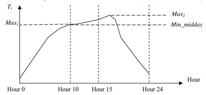
Figure 5.1 Single-Peak Pattern and Variables Describing Peaking Characteristics
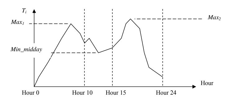
Figure 5.2 Double-Peak Pattern and Variables Describing Peaking Characteristics
Determining the presence of double peaks involves checking if both the morning peak traffic volume *Max*1 and afternoon peak traffic volume *Max*2 are larger than the minimum traffic volume between hour 10 and hour 15 (i.e., *Min\_midday*). Without losing generality, the smaller of the morning peak volume and afternoon peak volume is defined as
$$Min\_peak = \min\{Max_1, Max_2\}$$
(5-1)
The difference between *Min\_peak* and *Min\_midday* indicates the magnitude of the variation in midday traffic, which is defined as follows:
$$D_MinMax_MinMD = Min_peak - Min_midday$$
(5-2)
*Max* is defined as the maximum hourly traffic volume for an entire day:
$$Max = \max\{T_i\} \tag{5-3}$$
where *Ti* is the traffic for hour *i* (*i* = 1, 2, …, 24). *D\_MinMax\_MinMD* can be normalized by dividing it by *Max*. This determines the difference between the smaller of the peak traffic volumes and the minimum midday traffic volume as a percentage of the maximum daily hourly traffic:
$$PD\_MinMax\_MinMD = \frac{D\_MinMax\_MinMD}{Max}$$
(5-4)
An hourly traffic pattern is classified based on the value of *PD\_MinMax\_MinMD*. If *Min\_peak* is no larger than the *Min\_midday*, it means at least one of *Max*1 and *Max*2 is equal to the minimum hourly traffic between hours 10 and 15 (see Figure 5.1). In this case, *PD\_MinMax\_MinMD* is 0, which suggests that the traffic pattern has a single peak either at noon or in the early afternoon (seldom in the morning). Theoretically, it is possible to have two peaks, one morning or afternoon peak and one that may appear between hours 10 and 15. This will result in a TTMS being wrongly classified as having a single peak. This was not observed within the data from the 116 TTMSs, however.
If *PD\_MinMax\_MinMD* is larger than 0, at least two peaks exist. The value of *PD\_MinMax\_MinMD* indicates how large the difference is between the minimum peak traffic volume and the minimum midday traffic volume. If *PD\_MinMax\_MinMD* is small enough, the pattern is considered single-peaked. Four different scenarios are tested for cases of *PD\_MinMax\_MinMD* = 0.00, 0.10, 0.15, and 0.20 to investigate which one results in better models. It is possible that there may be a third peak during the midday period, but this happens rarely. Only two cases of a third peak have been observed, and they are still considered to share similarity with the double-peak TTMSs.
The hourly traffic patterns of three TTMSs with a single peak are plotted in Figure 5.3(a) for illustration purposes. The criterion applied to classify these TTMSs into the SP group is *PD\_MinMax\_MinMD* = 0. The traffic patterns of three other TTMSs with double peaks are shown in Figure 5.3(b). It may be seen this criterion has worked reasonably well.
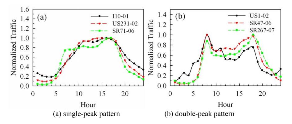
Figure 5.3 Hourly Traffic Variations for Selected TTMSs
Note that the hourly data used to classify traffic patterns are averaged from the full year data for all Wednesdays. It is assumed that the traffic patterns on Wednesdays are representative of those of the two other typical weekdays (Tuesdays and Thursdays). This has been confirmed by checking the traffic patterns of these two weekdays. The use of the average of full year data guarantees the smoothness of the data. It also reflects the overall traffic pattern on an annual basis.
From the application point of view, the short-term count data from PTMSs only cover a few days, such as a 72-hour period. The traffic variation over a short period may not be same as the pattern obtained from the averaged data for the whole year. This may cause difficulty in the application of this method. To verify that the SP or DP pattern based on annual average hourly traffic is similar to that of a short period count of 48 or 72 hours, the traffic patterns of selected TTMSs for selected weekdays are examined. It is found that most of the SP or DP traffic patterns remain unchanged, although some seasonal variations are observed. Figure 5.4(a) shows the hourly traffic patterns at site 530050 in the months of January, April, July, and October. This site exhibits single-peak traffic patterns that are generally consistent, even though the hourly traffic patterns within each month vary. Figure 5.4(b) shows the hourly traffic patterns at site 500054 during different seasons, also in the months of January, April, July, and October. These patterns are consistent with the double peak pattern.
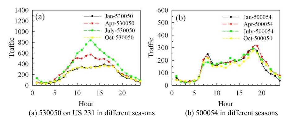
Figure 5.4 Hourly Traffic Pattern for TTMSs
Recognizing that individual hourly traffic patterns for the same location may not always be consistent, the classification results based on the cutoff criterion *PD\_MinMax\_MinMD* = 0 are determined for all of the TTMSs. There are a total of 1,472 hourly traffic patterns in the SP group and 10,564 in the DP group. For the TTMSs in the SP group, 53% of all of the individual day hourly traffic patterns are also single-peaked, while 89% in the DP group are also doublepeaked. One reason why averaged hourly traffic patterns may be different from everyday hourly traffic patterns is that traffic patterns also change with seasons. There is also the possibility that there is small randomness in the data. When the cutoff criterion is *PD\_MinMax\_MinMD* = 0.05, 74% of the SP group and 80% of the DP group agree with their classifications based on annual average hourly patterns.
After the TTMSs are classified into the SP and DP groups, regression models are developed to relate the seasonal factors with variables that describe land use, accessibility, and roadway characteristics. The modeling results are presented in the next two sections.
### **5.3 Single-Peak Models**
There are 33 TTMSs belonging to the SP group. The regression models for the SP group are given in Table 5.5.
For the SP group models, the R2 values are between 0.5529 and 0.9468. The only exception is the model for October, which is 0.4093. Overall, these R2 values are much higher than those of the models when the TTMSs are not separated into SP and DP groups.
The most significant variables are location variable *Dist1* and *SrtlP* and *SSHP*. Variables *SrtlP* and *SSHP* indicate that climate is an important factor. Moreover, they indicate that the same types of employment do not necessarily affect traffic seasonality during the same months in different climate zones.
Variable *Dist1* contributes an approximately 0.3 partial R2 to the March, April, June, and December models. Of the models for March, April, and December, the coefficient is negative. This suggests that the closer a count station is to an urban area, the more traffic it may experience during these months.
Variable *SRtlP* appears in seven models and contributes high partial R2 values to the January, July, August, and October models. For the January model, the coefficient of this variable is negative. For the other three models, the coefficient is positive. This indicates that retail-related employment in South Florida tends to increase traffic during January. In contrast, decreased traffic occurs during July, August, and October.
The *SSHP* variable is selected by four models. These are January, February, September, and October. The coefficients for January and February are negative, while those for September and October are positive. This indicates that the seasonal households in South Florida are active during the first two months of a year but not in September and October.
The variables *PPA18\_64* (age group 18-64) and *PPA22\_64* (age group 22-64) also appear frequently, with relatively high partial R2 in the January, February, June, and July models. They are correlated with an increase in traffic during winter time and contribute to a decrease in traffic during summer time.
Table 5.6 lists all of the variables included in the above models, along with their partial R2 values and the months for which they are significant. Tables 5.7 and 5.8 list all of the variables that have a partial R2 larger than 0.05. Table 5.7 sorts the variables by name and Table 5.8 by partial R2 value.
Table 5.5 Regression Models for the Single-Peak Group for Rural Areas
| h
M
t
on | Se
l
io
(
S
in
le
k
G
)
Fa
Eq
Pe
to
t
as
on
a
c
r
ua
n
g
a
ro
up | 2
R | 2
d
j.
A
R | R
M
S
E |
|-------------------|-------------------------------------------------------------------------------------------------------------------------------------------------------------------------------------------------------------------------------------------------------------------------------------------------------------------------------------------------------------------------------------------------------------------------------------------------------------------------------------------------------------------------------------------------------------------------------------------------------------------------------------------------------------------------------------------------------------------------------------------|------------------------|------------------------|------------------------|
| A
J
N | J
A
N_
S
F=
0.
8
5
5
7
2
0.
0
0
0
3
9
2
0
8×
In
de
d
is
2-
1.
1
6
5
3
0×
S
T
2
3
0.
4
8
1
5
8×
P
P
A
1
8_
6
4-
0.
0
0
2
6
8×
S
S
H
P
+
+
t
x
0.
0
0
6
2
3×
S
l
0.
0
1
1
1
1×
S
l
0.
4
1
8
3
6×
C
0.
0
0
3
9
2×
0.
0
0
2
6
9×
ho
l
Rt
P
H
P-
M
P-
Tr
P-
W
P
+
+
ot
se
um
an
d
0.
0
0
1
5
3×
E
P
0.
0
0
1
5
9×
M
P
+
an
u | 0.
9
4
6
8 | 0.
9
1
8
9 | 0.
0
2
4
4 |
| F
E
B | 6
l
F
E
B_
S
F=
0.
7
6
7
0
2
0.
4
5
8
9
9×
P
P
A
1
8_
4-
0.
0
0
0
9
2
9
3
2×
N
S
H
P-
0.
0
0
2
6
3×
S
S
H
P-
0.
0
0
6
9
8×
S
Rt
P-
+
0.
0
0
2
4
0×
W
ho
l
P | 0.
8
4
8
0 | 0.
8
1
9
8 | 0.
0
3
6
7 |
| M
A
R | M
A
R_
S
F=
0.
8
1
8
2
1-
0.
0
0
2
0
4×
T
F-
0.
0
0
0
0
0
2
1
4×
D
is
1
0.
3
5
3
6
0×
P
P
A
2
2_
6
4-
0.
0
0
1
2
0×
N
S
H
P-
+
t
0.
0
0
4
4
6×
S
l
0.
1
9
8
3
7×
0.
0
6
8
6
8×
S
Rt
P-
N
M
P-
M
P
se
um
se
um | 0.
8
2
9
9 | 0.
7
8
2
3 | 0.
0
3
1
0 |
| A
P
R | A
S
1.
0
0
5
0
3-
0.
0
0
0
0
0
1
1
2×
1-
4.
7
7
7
0
4
E-
7×
d
0.
0
0
0
7
7
1
6
2×
l
P
R_
F=
D
is
In
is
N
Rt
P
t
te
t
+
+
r
0.
4
1
4
1
0.
0
0
1
6
6×
0.
0
0
1
3
0×
7×
C
M
P-
Re
P-
M
P
t
se
um
s
an
u | 0.
7
0
3
5 | 0.
6
3
5
1 | 0.
0
2
5
3 |
| A
M
Y | 0.
9
8
2
4
9.
2
1
0
6
2
8
1-
6.
2
6
4
1
d
0.
0
0
4
9×
0.
0
0
1
2
4×
M
A
Y_
S
F=
5
E-
7×
D
is
5
E-
7×
In
is
7
Tr
P-
M
P
+
+
t
te
t
r
an
an
u | 0.
2
9
5
5 | 0.
4
8
9
0 | 0.
0
2
9
5 |
| J
U
N | 1.
2
2
4
3
0.
0
0
2
8
1×
0.
0
0
0
0
0
1
6
8×
1-
1.
4
1
2
8
1×
S
2
1
0.
9
2
8
9
9×
2
3-
J
U
N_
S
F=
7
T
F
D
is
T
S
T
+
+
+
t
0.
5
1
4
0
6×
P
P
A
2
2_
6
4 | 0.
6
8
0
5 | 0.
6
2
1
3 | 0.
0
4
0
6 |
| J
U
L | J
U
L_
S
F=
1.
1
2
1
7
5
0.
0
0
2
1
2×
T
F-
0.
0
0
0
3
9
1
8
9×
In
de
d
is
2
8.
1
1
2
8
E-
7×
In
d
is
0.
3
9
4
0
4×
P
P
A
1
8_
6
4
+
+
+
t
te
t-
x
r
0.
0
0
5
8
9×
S
Rt
l
P
0.
0
0
1
4
7×
M
P
+
an
u | 0.
7
8
7
2 | 0.
7
3
8
1 | 0.
0
3
7
1 |
| A
U
G | A
U
G_
S
F=
1.
0
7
5
9
5
0.
0
0
3
0
4×
T
F
7.
3
5
7
0
6
1
E-
7×
In
d
is
0.
2
3
1
2
1×
P
P
A
1
8_
6
4
0.
0
0
6
0
0×
S
Rt
l
P
+
+
+
+
te
t-
r
0.
0
2
6×
h
5
5
F
is
P | 0.
6
9
6
7 | 0.
6
4
0
5 | 0.
0
3
4
5 |
| S
E
P | S
S
1.
0
0
8
4
0.
4
4
8
S
2
1
0.
0
0
8
9
C
S
0.
0
0
1
2
1×
S
S
0.
0
0
4
1×
S
l
0.
0
0
8
2
6×
l
E
P_
F=
5
7
5×
T
5×
H
P
H
P
5
Rt
P
N
H
+
+
+
+
+
ot
h
P
0.
0
3
5
1
2×
F
is
P
0.
0
0
3
3
6×
Tr
P
+
+
an | 0.
8
3
0
5 | 0.
8
1
1
9 | 0.
0
2
2
5 |
| O
C
T | l
O
C
T_
S
F=
1.
0
2
0
7
5
0.
0
0
0
8
0
4
2
7×
S
S
H
P
0.
0
0
3
2
6×
S
Rt
P
+
+ | 0.
4
0
9
3 | 0.
3
6
9
9 | 0.
0
3
0
0 |
| N
O
V | de
d
N
O
V_
S
F=
1.
0
6
2
9
4
0.
0
5
2
4
0×
M
A
0.
0
0
0
5
1
4
6
8×
In
is
2-
1.
2
0
2
5
6×
S
T
2
3
0.
0
0
1
0
1×
Se
P
+
+
+
t
x
rv | 0.
7
3
3
0 | 0.
6
9
4
8 | 0.
0
2
7
1 |
| D
E
C | 6
l
D
E
C_
S
F=
0.
9
8
9
6
5-
0.
0
0
0
0
0
3
0
3×
D
is
1
0.
2
2
6
4
7×
P
P
A
1
8_
4
0.
0
1
0
9
8×
N
H
P
0.
0
1
0
0
3×
Rc
Se
P
+
+
+
t
ot
rv | 0.
6
5
6
0 | 0.
6
0
6
9 | 0.
0
3
8
3 |
| | | | | |
Table 5.6 Model Variables for Rural SP Group Sorted by Month and Partial R2 Value
| Partial
Variable
Month
R2
SRtlP
0.3413
JAN
PPA18_64
0.2069
JAN
SSHP
0.1173
JAN
WholP
0.0907
JAN
Indexdist2
0.0409
JAN
TranP
0.0313
JAN
ST23
0.0297
JAN
EdP
0.0275
JAN
ManuP
0.0181
JAN
0.0221
JAN
SHotlP
CMseumP
0.0208
JAN
SSHP
0.4765
FEB
WholP
0.1594
FEB | |
|--------------------------------------------------------------------------------------------------------------------------------------------------------------------------------------------------------------------------------------------------------------------------------------------------------------------------------------------------------------------------------------------|--|
| | |
| | |
| | |
| | |
| | |
| | |
| | |
| | |
| | |
| | |
| | |
| | |
| | |
| | |
| PPA18_64
0.1022
FEB | |
| SRtlP
0.0624
FEB | |
| NSHP
0.0474
FEB | |
| Dist1
0.3867
MAR | |
| NMseumP
0.1638
MAR | |
| SRtlP
0.0781
MAR | |
| NSHP
0.0625
MAR | |
| PPA22_64
0.0717
MAR | |
| TF
0.0345
MAR | |
| Variable | Partial
R2 | Month |
|------------|---------------|-------|
| SMseumP | 0.0326 | MAR |
| Dist1 | 0.2743 | APR |
| Interdist | 0.1279 | APR |
| ManuP | 0.0769 | APR |
| RestP | 0.0992 | APR |
| CMseumP | 0.0733 | APR |
| NRtlP | 0.052 | APR |
| TranP | 0.1901 | MAY |
| Interdist | 0.1924 | MAY |
| ManuP | 0.0909 | MAY |
| Dist1 | 0.0795 | MAY |
| Dist1 | 0.2853 | JUN |
| PPA22_64 | 0.1752 | JUN |
| ST21 | 0.0886 | JUN |
| TF | 0.0769 | JUN |
| ST23 | 0.0544 | JUN |
| ManuP | 0.2628 | JUL |
| SRtlP | 0.1595 | JUL |
| PPA18_64 | 0.1402 | JUL |
| Indexdist2 | 0.0935 | JUL |
| Interdist | 0.08 | JUL |
| TF | 0.0511 | JUL |
| | | |
| Variable | Partial
R2 | Month |
|------------|---------------|-------|
| SRtlP | 0.2331 | AUG |
| Interdist | 0.1622 | AUG |
| TF | 0.1278 | AUG |
| FishP | 0.0889 | AUG |
| PPA18_64 | 0.0847 | AUG |
| SSHP | 0.3317 | SEP |
| CSHP | 0.2332 | SEP |
| SRtlP | 0.083 | SEP |
| NHotlP | 0.0809 | SEP |
| FishP | 0.0571 | SEP |
| ST21 | 0.0362 | SEP |
| TranP | 0.031 | SEP |
| SSHP | 0.2954 | OCT |
| SRtlP | 0.1139 | OCT |
| Indexdist2 | 0.277 | NOV |
| ServP | 0.199 | NOV |
| ST23 | 0.1645 | NOV |
| MA | 0.0924 | NOV |
| Dist1 | 0.3387 | DEC |
| NHotlP | 0.1597 | DEC |
| RcServP | 0.0879 | DEC |
| PPA18_64 | 0.0698 | DEC |
| | | |
Table 5.7 Model Variables for Rural SP Group Sorted by Name and Partial R2 Value
| Variable | Partial R2 | Month |
|------------|------------|-------|
| CMseumP | 0.0733 | APR |
| CSHP | 0.2332 | SEP |
| Dist1 | 0.3867 | MAR |
| Dist1 | 0.3387 | DEC |
| Dist1 | 0.2853 | JUN |
| Dist1 | 0.2743 | APR |
| Dist1 | 0.0795 | MAY |
| FishP | 0.0889 | AUG |
| FishP | 0.0571 | SEP |
| Indexdist2 | 0.277 | NOV |
| Indexdist2 | 0.0935 | JUL |
| Interdist | 0.1924 | MAY |
| Interdist | 0.1622 | AUG |
| Interdist | 0.1279 | APR |
| Interdist | 0.08 | JUL |
| MA | 0.0924 | NOV |
| ManuP | 0.2628 | JUL |
| ManuP | 0.0909 | MAY |
| Variable | Partial R2 | Month |
|----------|------------|-------|
| ManuP | 0.0769 | APR |
| NHotlP | 0.1597 | DEC |
| NHotlP | 0.0809 | SEP |
| NMseumP | 0.1638 | MAR |
| NRtlP | 0.052 | APR |
| NSHP | 0.0625 | MAR |
| PPA18_64 | 0.2069 | JAN |
| PPA18_64 | 0.1402 | JUL |
| PPA18_64 | 0.1022 | FEB |
| PPA18_64 | 0.0847 | AUG |
| PPA18_64 | 0.0698 | DEC |
| PPA22_64 | 0.1752 | JUN |
| PPA22_64 | 0.0717 | MAR |
| RcServP | 0.0879 | DEC |
| RestP | 0.0992 | APR |
| ServP | 0.199 | NOV |
| SRtlP | 0.3413 | JAN |
| SRtlP | 0.2331 | AUG |
| | | |
| Variable | Partial R2 | Month |
|----------|------------|-------|
| SRtlP | 0.1595 | JUL |
| SRtlP | 0.1139 | OCT |
| SRtlP | 0.083 | SEP |
| SRtlP | 0.0781 | MAR |
| SRtlP | 0.0624 | FEB |
| SSHP | 0.4765 | FEB |
| SSHP | 0.3317 | SEP |
| SSHP | 0.2954 | OCT |
| SSHP | 0.1173 | JAN |
| ST21 | 0.0886 | JUN |
| ST23 | 0.1645 | NOV |
| ST23 | 0.0544 | JUN |
| TF | 0.1278 | AUG |
| TF | 0.0769 | JUN |
| TF | 0.0511 | JUL |
| TranP | 0.1901 | MAY |
| WholP | 0.1594 | FEB |
| WholP | 0.0907 | JAN |
| | | |
Table 5.8 Model Variables for Rural SP Group Sorted by Partial R2 Value
| Variable | Partial R2 | Month |
|------------|------------|-------|
| SSHP | 0.4765 | FEB |
| Dist1 | 0.3867 | MAR |
| SRtlP | 0.3413 | JAN |
| Dist1 | 0.3387 | DEC |
| SSHP | 0.3317 | SEP |
| SSHP | 0.2954 | OCT |
| Dist1 | 0.2853 | JUN |
| Indexdist2 | 0.277 | NOV |
| Dist1 | 0.2743 | APR |
| ManuP | 0.2628 | JUL |
| CSHP | 0.2332 | SEP |
| SRtlP | 0.2331 | AUG |
| PPA18_64 | 0.2069 | JAN |
| ServP | 0.199 | NOV |
| Interdist | 0.1924 | MAY |
| TranP | 0.1901 | MAY |
| PPA22_64 | 0.1752 | JUN |
| ST23 | 0.1645 | NOV |
| | | |
| Variable | Partial R2 Month | |
|------------|------------------|-----|
| NMseumP | 0.1638 | MAR |
| Interdist | 0.1622 | AUG |
| NHotlP | 0.1597 | DEC |
| SRtlP | 0.1595 | JUL |
| WholP | 0.1594 | FEB |
| PPA18_64 | 0.1402 | JUL |
| Interdist | 0.1279 | APR |
| TF | 0.1278 | AUG |
| SSHP | 0.1173 | JAN |
| SRtlP | 0.1139 | OCT |
| PPA18_64 | 0.1022 | FEB |
| RestP | 0.0992 | APR |
| Indexdist2 | 0.0935 | JUL |
| MA | 0.0924 | NOV |
| ManuP | 0.0909 | MAY |
| WholP | 0.0907 | JAN |
| FishP | 0.0889 | AUG |
| ST21 | 0.0886 | JUN |
| | | |
| Variable | Partial R2 Month | |
|-----------|------------------|-----|
| RcServP | 0.0879 | DEC |
| PPA18_64 | 0.0847 | AUG |
| SRtlP | 0.083 | SEP |
| NHotlP | 0.0809 | SEP |
| Interdist | 0.08 | JUL |
| Dist1 | 0.0795 | MAY |
| SRtlP | 0.0781 | MAR |
| ManuP | 0.0769 | APR |
| TF | 0.0769 | JUN |
| CMseumP | 0.0733 | APR |
| PPA22_64 | 0.0717 | MAR |
| PPA18_64 | 0.0698 | DEC |
| NSHP | 0.0625 | MAR |
| SRtlP | 0.0624 | FEB |
| FishP | 0.0571 | SEP |
| ST23 | 0.0544 | JUN |
| NRtlP | 0.052 | APR |
| TF | 0.0511 | JUL |
| | | |
### **5.4 Double-Peak Models**
There are 83 TTMSs in the DP group. The regression models for the 12 MSFs are given in Table 5.9.
For the DP group models, the most significant variables are *Dist1*, *SRtlP*, and *SSHP*. The *SRtlP* variable contributes the largest partial R2 value to the January, February, August, and September models. The coefficients in the January and February models are negative. Those for August and September are positive. This indicates that retail-related employment in South Florida tends to generate more traffic in January and February and does the opposite in August and September.
The variable *SSHP* is present in the March model with a negative coefficient and in the May and October models with a positive coefficient. This indicates that the traffic generated by seasonal households in South Florida is more noticeable in March, whereas these households have less of an impact on traffic in May and October.
The variable *Dist1* appears in eight models: January, February, March, May, June, July, November, and December. The coefficients in the June and July models are positive. They are negative for the other six models. This suggests that, for a count station near an urban area, traffic tends to decrease in June and July, but increases for the other six months.
Table 5.10 lists all of the variables included in the above models, along with their partial R2 value and the months for which they significant. Table 5.11 and 5.12 list all of the variables that have a partial R2 larger than 0.05. Table 5.11 sorts the variables by name and Table 5.12 by partial R2 value.
Table 5.9 Regression Models for Rural DP Group
| h
Se
l
io
(
b
le
k
G
)
A
d
j.
S
M
Fa
Eq
D
Pe
R
R
R
M
t
to
t
on
as
on
a
c
r
ua
n
ou
a
ro
up
A
S
1.
1
4
6
8
8-
0.
0
0
0
0
0
1
6
4
1-
0.
0
0
0
4
0
2
h
d
J
N
F=
D
is
7
5
Be
is
×
t
×
t-
ac
A
J
N
_
0.
0
0
4
8
h
0.
0
0
2
3
3
0.
0
0
3
0
l
0.
0
1
4
4
l
0.
0
0
0
2
9
3
8
0.
6
0
9
0.
3
0
0.
0
4
6
7
R
H
ig
N
S
H
P-
5
S
R
P
5
C
H
P-
5
Se
P
5
5
7
+
+
×
t_
×
×
t
×
t
×
o
rv
1.
1
2
6-
0.
0
0
0
0
0
1
1
1
1-
0.
0
0
3
1
0
1.
2
8
0
8
1
2
2
0.
0
0
2
F
E
B_
S
F=
7
7
D
is
R
E
T
I
R
E-
S
T
7
5
N
S
H
P-
+
×
t
×
×
×
F
E
B
0.
0
0
6
l
0.
6
2
9
8
0.
6
0
0.
0
4
5
5
S
R
P
5
7
5
×
t
A
S
1.
0
1
3
0
8-
0.
0
2
0
0
3
A
-8
8
6
8
0
1
1-
0.
0
0
0
0
1
de
d
2-
M
R_
F=
P
E-
7
D
is
5
5
5
In
is
×
×
t
×
t
x
A
M
R
0.
0
0
3
6
h-
0.
0
0
2
6
0.
0
0
6
8
8
l
0.
8
4
0.
1
9
0.
0
3
7
R
H
ig
5
S
S
H
P-
S
H
P
5
7
5
5
5
×
t_
×
×
t
o
A
P
R
A
S
0.
9
8
9
0
8-
0.
0
1
5
0
6
A
-0
0
0
3
0
4
h
0.
0
0
0
4
3
4
2
4
d
0.
2
5
8
1
0.
2
2
9
9
0.
0
2
6
P
R_
F=
P
R
H
ig
E
P
+
×
×
t_
×
M
A
Y
M
A
Y_
S
F=
0.
9
6
9
3
0
3.
9
9
7
4
9
1
E-
7
D
is
1
0.
0
0
2
1
3
S
S
H
P
0.
0
0
9
1
0
C
H
l
P
0.
2
8
3
0
0.
2
5
5
8
0.
0
3
0
+
+
+
×
t
×
×
t
o
J
U
N
S
F=
0.
8
8
9
5
0-
0.
0
4
7
9
5
C
O
0.
0
0
0
0
0
1
5
4
D
is
1
0.
0
0
0
5
7
7
7
4
Be
h
d
is
+
t
+
t
×
×
×
ac
J
U
N
_
0.
0
0
5
2
8
R
E
T
I
R
E-
0.
0
0
4
0
4
R
Lo
-0
0
0
2
4
8
N
S
H
P
0.
5
2
7
8
0.
4
9
0
6
0.
0
4
6
+
×
×
t_
×
w
J
U
L_
S
F=
0.
7
8
9
9
1
0.
0
0
0
0
0
1
8
8
D
is
1
0.
0
0
1
0
8
Be
h
d
is
0.
0
0
7
5
0
R
E
T
I
R
E
+
+
+
t
t
×
×
×
ac
J
U
L
0.
0
0
4
8
7
R
Lo
0.
7
1
9
9
2
P
P
A
1
8_
2
1-
0.
0
0
3
7
7
N
S
H
P-
0.
0
1
5
1
2
C
H
l
P
0.
0
0
2
2
0
A
i
P
t_
+
t
+
×
×
×
×
×
w
o
g
r
0.
0
0
6
4
6
Se
0.
0
0
2
5
1
in
0.
7
1
2
2
0.
6
7
2
2
0.
0
4
7
Rc
P
M
P
+
+
×
×
rv
e
A
U
G
S
F=
0.
9
6
4
5
3
8.
3
8
1
7
1
9
E-
7
D
is
1
0.
2
4
5
7
5
P
P
A
6
5u
0.
0
0
8
1
6
S
R
l
P
+
+
+
t
t
×
×
×
p
A
U
G
_
0.
0
0
4
5
6
Rc
Se
P
0.
0
0
2
5
9
M
in
P
0.
5
6
8
6
0.
5
4
0
6
0.
0
4
6
+
+
×
×
rv
e
S
E
P
S
E
S
F=
0.
9
9
0
5
7
0.
0
0
2
2
0
T
F
0.
0
0
3
9
4
R
H
h
0.
0
0
5
1
1
S
R
l
P
0.
0
0
3
4
3
Rc
Se
P
0.
4
7
1
7
0.
4
4
4
6
0.
0
4
0
+
+
+
t
+
×
×
×
×
rv | | | | |
|-----------------------------------------------------------------------------------------------------------------------------------------------------------------------------------------------------------------------------------------------------------------------------------------------------------------------------------------------------------------------------------------------------------------------------------------------------------------------------------------------------------------------------------------------------------------------------------------------------------------------------------------------------------------------------------------------------------------------------------------------------------------------------------------------------------------------------------------------------------------------------------------------------------------------------------------------------------------------------------------------------------------------------------------------------------------------------------------------------------------------------------------------------------------------------------------------------------------------------------------------------------------------------------------------------------------------------------------------------------------------------------------------------------------------------------------------------------------------------------------------------------------------------------------------------------------------------------------------------------------------------------------------------------------------------------------------------------------------------------------------------------------------------------------------------------------------------------------------------------------------------------------------------------------------------------------------------------------------------------------------------------------------------------------------------------------------------------------------------------------------------------------------------------------------------------------------------------------------------------------------------------------------------------------------------------------------------------------------------------------------------------------------------------------------------------------------------------------------------------------------------------------------------------------------------------------------------------------------------------------------------------------------------------------------------------------------------------------------------------------------------------------------------------------------------------------------------------------------------------------------------------------------------------------------------------------------------------------------------------------------------------------------------------------------------------------------------------------------------------------------------------------------------------------------------------------------------------------------------------------------------------------------------------------------------------------------------------------------------------------------------------------------------------------------------------------------------------------------------------------------------------------------------------------------------------------------------------------------------------------------------------------------------------------------------------------------------------------------------------------------------------------------------------------------------------------------------------------------------------------------------------------------------------------------------------------------------------------------------------------------------------------------------------------------------------------------------------------------------------------------------------------------------------------------------------------------------------------------------------------------------------------------------------------------------------------------------------------------------------------------------------------------------------------------------------------------------------------------------------------------------------------------------------------------------------------------------------------------------------------------------------------------------------------------------------------------------------------------------------------------------------------------------------------------------------------------------------------------------------------------------------------------------------------------------------------------------------|----------------|---|---|---|
| | | 2 | 2 | E |
| | | | | |
| | | | | 4 |
| | | | | |
| | | | | 3 |
| | | | | |
| | | | | 9 |
| | | | | 9 |
| | | | | 6 |
| | | | | |
| | | | | 4 |
| | | | | |
| | | | | |
| | | | | 8 |
| | | | | |
| | | | | 0 |
| | P_
ig
t_ | | | 5 |
| O
C
T
O
C
T_
S
F=
1.
0
1
0
0
7
0.
0
1
8
5
3
P
A
0.
0
0
2
3
4
S
S
H
P
0.
0
0
7
5
5
S
H
l
P
0.
2
6
9
0
0.
2
4
1
2
0.
0
3
5
+
+
+
t
×
×
×
o | | | | 6 |
| N
O
V
N
O
V_
S
F=
1.
0
5
7
4
8-
0.
0
0
0
0
0
1
4
9
D
is
1-
0.
0
0
0
6
6
9
7
3
Be
h
d
is
0.
5
4
4
1
3
S
T
2
3
0.
3
4
7
6
0.
3
2
2
9
0.
0
4
3
+
×
t
×
t
×
ac | | | | 2 |
| h
d
D
E
C
D
E
C_
S
F=
1.
0
7
9
9
7-
0.
0
0
0
0
0
1
4
9
D
is
1-
0.
0
0
0
7
1
9
5
8
Be
is
0.
0
0
2
9
4
N
S
H
P
0.
3
8
1
3
0.
3
5
7
8
0.
0
5
1
+
×
t
×
t
×
ac | | | | 7 |
Table 5.10 Model Variables for Rural DP Group Sorted by Month and Partial R2 value
| Partial R2 | Month |
|------------|-------|
| 0.3306 | JAN |
| 0.0994 | JAN |
| 0.0499 | JAN |
| 0.0512 | JAN |
| 0.0258 | JAN |
| 0.024 | JAN |
| 0.0286 | JAN |
| 0.3832 | FEB |
| 0.0857 | FEB |
| 0.069 | FEB |
| 0.052 | FEB |
| 0.0399 | FEB |
| 0.3411 | MAR |
| 0.1216 | MAR |
| 0.0409 | MAR |
| 0.0337 | MAR |
| 0.0249 | MAR |
| 0.0225 | MAR |
| | |
| Variable | Partial R2 | Month |
|-----------|------------|-------|
| Rt_High | 0.1602 | APR |
| PA | 0.0598 | APR |
| EdP | 0.0381 | APR |
| SSHP | 0.1688 | MAY |
| Dist1 | 0.0664 | MAY |
| CHotlP | 0.0479 | MAY |
| Dist1 | 0.3032 | JUN |
| RETIRE | 0.0952 | JUN |
| NSHP | 0.0309 | JUN |
| CO | 0.0349 | JUN |
| Beachdist | 0.0315 | JUN |
| Rt_Low | 0.0322 | JUN |
| Dist1 | 0.2465 | JUL |
| NSHP | 0.0691 | JUL |
| Beachdist | 0.086 | JUL |
| AgriP | 0.0478 | JUL |
| RcServP | 0.0358 | JUL |
| MineP | 0.0291 | JUL |
| | | |
| Variable | Partial R2 | Month |
|-----------|------------|-------|
| | | |
| SRtlP | 0.4058 | AUG |
| MineP | 0.0423 | AUG |
| PPA65up | 0.0393 | AUG |
| Dist1 | 0.0476 | AUG |
| RcServP | 0.0337 | AUG |
| SRtlP | 0.354 | SEP |
| Rt_High | 0.0451 | SEP |
| TF | 0.0429 | SEP |
| RcServP | 0.0296 | SEP |
| SSHP | 0.1435 | OCT |
| SHotlP | 0.0763 | OCT |
| PA | 0.0492 | OCT |
| Dist1 | 0.1976 | NOV |
| Beachdist | 0.1137 | NOV |
| ST23 | 0.0364 | NOV |
| Dist1 | 0.2414 | DEC |
| Beachdist | 0.0656 | DEC |
| NSHP | 0.0742 | DEC |
Table 5.11 Model Variables for Rural DP Group Sorted by Name and Partial R2 Value
| Variable | Partial R2 | Month | |
|-----------|------------|-------|--|
| Beachdist | 0.1137 | NOV | |
| Beachdist | 0.086 | JUL | |
| Beachdist | 0.0656 | DEC | |
| Dist1 | 0.3032 | JUN | |
| Dist1 | 0.2465 | JUL | |
| Dist1 | 0.2414 | DEC | |
| Dist1 | 0.1976 | NOV | |
| Dist1 | 0.1216 | MAR | |
| Dist1 | 0.0994 | JAN | |
| Variable | Partial R2 | Month | | | | |
|----------|------------|-------|--|--|--|--|
| Dist1 | 0.0857 | FEB | | | | |
| Dist1 | 0.0664 | MAY | | | | |
| PA | 0.0598 | APR | | | | |
| NSHP | 0.0742 | DEC | | | | |
| NSHP | 0.0691 | JUL | | | | |
| NSHP | 0.052 | FEB | | | | |
| RETIRE | 0.0952 | JUN | | | | |
| RETIRE | 0.069 | FEB | | | | |
| SHotlP | 0.0763 | OCT | | | | |
| | | | | | | |
| Value | | | | | | |
|----------|--------|------------|--|--|--|--|
| Variable | | Month | | | | |
| SRtlP | 0.4058 | AUG | | | | |
| SRtlP | 0.3832 | FEB | | | | |
| SRtlP | 0.354 | SEP | | | | |
| SRtlP | 0.3306 | JAN | | | | |
| SSHP | 0.3411 | MAR | | | | |
| SSHP | 0.1688 | MAY | | | | |
| SSHP | 0.1435 | OCT | | | | |
| Rt_High | 0.1602 | APR | | | | |
| Rt_High | 0.0512 | JAN | | | | |
| | | Partial R2 | | | | |
Table 5.12 Model Variables for Rural DP Group Sorted by Partial R2 Value
| Variable | Partial R2 | Month |
|----------|------------|-------|
| SRtlP | 0.4058 | AUG |
| SRtlP | 0.3832 | FEB |
| SRtlP | 0.354 | SEP |
| SSHP | 0.3411 | MAR |
| SRtlP | 0.3306 | JAN |
| Dist1 | 0.3032 | JUN |
| Dist1 | 0.2465 | JUL |
| Dist1 | 0.2414 | DEC |
| Dist1 | 0.1976 | NOV |
| Variable | Partial R2 | Month |
|-----------|------------|-------|
| SSHP | 0.1688 | MAY |
| Rt_High | 0.1602 | APR |
| SSHP | 0.1435 | OCT |
| Dist1 | 0.1216 | MAR |
| Beachdist | 0.1137 | NOV |
| Dist1 | 0.0994 | JAN |
| RETIRE | 0.0952 | JUN |
| Beachdist | 0.086 | JUL |
| Dist1 | 0.0857 | FEB |
| | | |
| Variable | Partial R2 | Month |
|-----------|------------|-------|
| SHotlP | 0.0763 | OCT |
| NSHP | 0.0742 | DEC |
| NSHP | 0.0691 | JUL |
| RETIRE | 0.069 | FEB |
| Dist1 | 0.0664 | MAY |
| Beachdist | 0.0656 | DEC |
| PA | 0.0598 | APR |
| NSHP | 0.052 | FEB |
| Rt_High | 0.0512 | JAN |
### **6. PRELIMINARY INVESTIGATION OF SEASON FACTOR ASSIGNMENT**
The models described in Chapters 4 and 5 indicate that there is a relationship between the monthly seasonal factors and land use variables. Even though the models cannot be used to directly predict the monthly seasonal factors, they provide likely connections between the seasonal factors and the various variables modeled. These variables may be used to develop a metric to determine which TTMS(s) may be used for the assignment of seasonal factors to a coverage count site. This metric is based on the similarity between land use and other characteristics. This chapter describes a preliminary investigation to explore a simple and practical assignment method. Results from the application of this method are also described. Section 6.1 explains the methodology used for assignment. Sections 6.2 through 6.4 present assignment results in urban areas from three different assignment strategies.
### **6.1 Methodology for Measuring Similarity between Two Count Sites**
In Florida, the current practice for assigning seasonal factors to coverage counts is to create seasonal factor groups and to use the group averages as the seasonal factors. Next, these seasonal groups are assigned to coverage count sites. Their averaged seasonal factors are then applied to convert ADT to AADT. During the first phase of this project, a fuzzy decision tree was developed (Zhao 2004, Li *et al*. 2006). It was used for classifying a count site based on the value of selected variables (or decision variables) that were identified in regression analysis. In constructing the fuzzy decision tree, those TTMSs that have already been grouped are used. The group they belong to is considered a class that the fuzzy decision tree should be able to correctly define. This definition is based on the values of a set of decision variables. The values of these decision variables are computed for each TTMS. One variable is selected at a time. Based on the values of a given variable of all of the TTMSs, a dividing point is then determined to classify the TTMSs into two groups: One group's variable values are smaller than the value defining the dividing point, and the other group's are larger. Next, a new variable is selected and each of the two groups is further divided into two new groups. This process repeats until all of the TTMSs are classified. That is, each group only has TTMSs that belong to the same seasonal factor group. A perfectly built tree should result in all of the TTMSs of the same seasonal factor group also being classified into the same group by the decision tree. The decision tree, therefore, is defined by the sequence of the variables applied at each step of classification and the variable values at the dividing points. Furthermore, a fuzzy decision tree allows a fuzzy range around the dividing point. If the value of a decision variable is outside this fuzzy range, a TTMS is classified with 100% probability into one of the two subgroups. Otherwise, a TTMS is classified as a member of both subgroups with a probability of less than 100%.
In the Phase 1 study, such a tree was constructed successfully, meaning that TTMSs belonging to the same seasonal factor group were also classified by the decision tree into the same group. However, the tree was not tested for application. This is because testing required MSFs data that were not already used in constructing the fuzzy decision tree, and there were no additional TTMSs that could be used for that purpose. This continues to be a problem because the number of available TTMSs is limited. The geographic area that must be covered is very large, and there are many seasonal factor groups. This creates a demand for even more test data with which to test the entire decision tree.
In addition to the lack of TTMS data for testing a fuzzy decision tree, this method also had a few other limitations. One was that there could be too much fuzziness in the classification. Although all of the TTMSs were classified into their correct groups, their membership in the group they belong to may have been incomplete. This means that the probability of their belonging was less than 100%. Additionally, because TTMSs may be classified multiple times by different variables, their membership in a group may have been low. This is because the TTMSs in different groups were not completely distinct in either their seasonal factors or land use characteristics. Another limitation was that the tree structure highly depends on seasonal factor grouping. Any changes in seasonal factor grouping will lead to changes in the tree structure. This would not be a concern if there were no uncertainty in the seasonal factor grouping process. However, the SF grouping process involves much judgment. Furthermore, there is no guarantee that the TTMSs in the same SF group will actually share the same characteristics represented by the decision variables.
In this study, a different approach is developed. This approach is based on the idea that if the variables identified in the regression analysis are the underlying causes for the seasonal traffic variations, they may be used to directly link one count station to a TTMS based on the similarity between their variable values. This is determined by a similarity score, *S*. This score is calculated based on a selected set of variables that are identified during regression analyses. To measure the similarity, the differences between the values of each of the variables are first computed for the two count stations. These differences are then weighted by the regression partial R2 values corresponding to the variables, normalized by the maximum value of the variables, and summarized. *S* for two count stations *i* and *j* may be expressed as follows:
$$S_{ij} = \sum_{k=1}^{p} \frac{\left| V_{ki} - V_{kj} \right| \times PR_k}{\max_{k} \left\{ V_k \right\}}$$
$$\tag{6-1}$$
where
*Sij* = the similarity score defined for count stations *i* and *j* (*i* ≠ *j*),
*Vki* = the value of the *k*th variable in the 12-month models for count station *i*,
*Vkj* = the value of the *k*th variable in the 12-month models for count station *j*,
*PRk* = the partial R2 for the *k*th variable, and
*max*(*Vk*) = the maximum value for the variable *Vk* among all TTMSs.
Recall that there are 12 regression equations in each model set. Any variables may appear repeatedly in different equations and, therefore, may be associated with different R2 values. Hence, the similarity score for the whole year is summed from the 12 month scores.
Using the above definition, similarity scores can be computed for each pair of count stations. The goal of the assignment here is to identify one or more best matched TTMSs for any given shortterm count site. If multiple TTMSs are matched to a given count site, they may be ranked based on their similarity scores as the first best match, second best match, and so on.
To test this methodology, TTMSs in the urban areas are used to find matches. Because the MSFs for these TTMSs are already known, it is possible to evaluate whether this method provides satisfactory assignment results. A particular assignment result that matches a TTMS *j* to a count site *i* is evaluated based on the square root of the sum of the mean square of the 12 month seasonal factor differences. That is,
$$e_{ij} = \sqrt{\frac{1}{12} \sum_{m=1}^{12} \left( \frac{MSF_{mi} - MSF_{mj}}{MSF_{mi}} \right)^2}$$
(6-2)
where
*eij =* a measure of difference between the monthly seasonal factors of count site *i* and *j* being compared,
*MSFmi* = the monthly seasonal factor for count site *i* for month *m*, and
*MSFmj* = the monthly seasonal factor for count site *j* for month *m*.
A good match should have a small error.
In the next section, the above method is applied to TTMSs in urban areas.
### **6.2 Urban TTMS Assignment within Model Regions**
The urban area TTMSs are modeled for three different regions: North, Central, and South Florida. There is one set of models for each of the three regions. The assignment is conducted within each region for TTMSs in all three regions. In other words, only TTMSs within the same region are considered as the candidates for any given count site. For any TTMS within a region, which is tested here as a short-count site, all of the TTMSs in the same region are treated as potential candidates. Their similarity scores are then computed.
The variables used to calculate the similarity scores for TTMSs are summarized in Table 6.1*.* These variables are thought to be significant for each of the model regions based on the regression analyses described in Chapter 4. The definition of the variables can be found in Section 4.1.
Table 6.1 Variable Sets Used for Assignment for Model Regions
| Model Region | Variables |
|--------------|------------------------------------------------------------------|
| North | EdP, FishP, FR, HotlP, LEG, MA, MseumP, OffP, RcServP, RestP, |
| | RETIRE, SHP, ST1, ST22, ST23, Rt_Low, SU, TranP, and WholP |
| Central | AgriP, CO, DISN, EdP, MA, MInc, MineP, MseumP, OffP, PA, |
| | RETIRE, RtlP, ServP, SHP, ST22, ST23, Rt_High, Rt_Low, and TranP |
| South | AgriP, HotlP, MA, ManuP, MseumP,RcServP, RETIRE, SHP, ST1, |
| | ST23, and SU |
The first five best matching TTMSs are presented. Table 6.2 shows the assignment results for each TTMS in North Florida, Table 6.3 for those in Central Florida, and Table 6.4 for those in South Florida. The column *Test Sites* gives the identification number of a TTMS. This TTMS is treated as a short-term count site. The next five columns list the first five best matching sites based on their similarity scores.
Table 6.2 Assignment Results for TTMSs in North Florida
| | Bets Matching Sites | | | | |
|------------|---------------------|--------|--------|--------|--------|
| Test Sites | 1st | 2nd | 3rd | 4th | 5th |
| 260323 | 550208 | 550207 | 550226 | 550300 | 550206 |
| 290286 | 729923 | 290320 | 480156 | 720161 | 509940 |
| 550206 | 550300 | 550208 | 550212 | 559908 | 550207 |
| 559908 | 550212 | 550206 | 260185 | 550300 | 550226 |
| 720161 | 729923 | 720172 | 290320 | 720171 | 480159 |
| 780329 | 480282 | 720172 | 570250 | 480159 | 110246 |
| 550207 | 550226 | 550300 | 550208 | 550206 | 550209 |
| 460315 | 360317 | 509940 | 530117 | 720172 | 360264 |
| 530117 | 460315 | 360317 | 110246 | 509940 | 480282 |
| 460308 | 720121 | 570318 | 720062 | 480159 | 740182 |
| 080283 | 360317 | 730335 | 460315 | 730292 | 760105 |
| 360264 | 460315 | 730335 | 360317 | 020044 | 080283 |
| 110246 | 480282 | 780311 | 360317 | 570250 | 720172 |
| 580261 | 570318 | 729923 | 460308 | 780311 | 720109 |
| 729923 | 720161 | 780311 | 570318 | 729914 | 720172 |
| 550212 | 550206 | 559908 | 260185 | 550300 | 550226 |
| 730335 | 080283 | 360264 | 020044 | 360317 | 730292 |
| 260185 | 550212 | 559908 | 550206 | 720109 | 780311 |
| 730292 | 360317 | 730335 | 080283 | 489924 | 760105 |
| 760105 | 360317 | 730335 | 080283 | 460315 | 730292 |
| 290320 | 720161 | 729923 | 290286 | 720171 | 570318 |
| 509940 | 780311 | 460315 | 720172 | 360317 | 480159 |
| 550151 | 550304 | 550300 | 550207 | 550226 | 550208 |
| 550208 | 550300 | 550206 | 550207 | 550226 | 550212 |
| 550209 | 550226 | 550207 | 550300 | 260185 | 480282 |
| 550213 | 550206 | 550300 | 550208 | 559908 | 550212 |
| 550226 | 550207 | 550300 | 550209 | 550208 | 550206 |
| 720062 | 720121 | 460308 | 570167 | 480159 | 720172 |
| 720121 | 570167 | 720062 | 460308 | 480159 | 480325 |
| 720172 | 480159 | 780311 | 480282 | 570250 | 460308 |
| 720216 | 489924 | 460308 | 480159 | 729914 | 720121 |
| 740182 | 360249 | 460308 | 720109 | 570318 | 589937 |
| 780311 | 720172 | 480159 | 509940 | 360249 | 720109 |
| 720109 | 589937 | 460308 | 740182 | 360249 | 480159 |
| 720171 | 720161 | 489924 | 729914 | 720216 | 290320 |
| 550300 | 550206 | 550208 | 550207 | 550226 | 550212 |
| 550304 | 720171 | 550300 | 550151 | 550208 | 550207 |
| 729914 | 489924 | 729923 | 720216 | 780311 | 720171 |
| 460166 | 570293 | 460305 | 780329 | 760105 | 600168 |
| 460305 | 720161 | 290320 | 720171 | 580261 | 729923 |
| 480159 | 720172 | 360249 | 460308 | 780311 | 720109 |
| 480282 | 720172 | 570250 | 110246 | 480159 | 360249 |
| 480325 | 570167 | 720121 | 589937 | 720109 | 720062 |
| | Bets Matching Sites | | | | |
|------------|---------------------|--------|--------|--------|--------|
| Test Sites | 1st | 2nd | 3rd | 4th | 5th |
| 570250 | 720172 | 480282 | 360249 | 740182 | 110246 |
| 570293 | 290320 | 720161 | 550151 | 720171 | 460305 |
| 589937 | 720109 | 570167 | 720121 | 460308 | 480325 |
| 570318 | 460308 | 480159 | 720109 | 360249 | 780311 |
| 489924 | 720216 | 729914 | 720172 | 480159 | 780311 |
| 480156 | 460308 | 480159 | 570318 | 360249 | 720172 |
| 570167 | 720121 | 460308 | 720062 | 480325 | 589937 |
| 600168 | 760105 | 460308 | 720062 | 720172 | 480159 |
| 710189 | 720121 | 720062 | 570167 | 480156 | 480159 |
| 080294 | 110177 | 760105 | 360264 | 730335 | 020044 |
| 110177 | 080294 | 020044 | 360264 | 730335 | 760105 |
| 360249 | 740182 | 480159 | 780311 | 720109 | 570250 |
| 020044 | 730335 | 360317 | 360264 | 080283 | 730292 |
| 360317 | 460315 | 080283 | 509940 | 110246 | 530117 |
Table 6.3 Assignment Results for TTMSs in Central Florida
| | Bets Matching Sites | | | | |
|------------|---------------------|--------|--------|--------|--------|
| Test Sites | 1st | 2nd | 3rd | 4th | 5th |
| 100106 | 109926 | 100224 | 100194 | 109922 | 750196 |
| 100321 | 770102 | 100162 | 750154 | 750038 | 150295 |
| 150302 | 109922 | 100194 | 100224 | 750130 | 109926 |
| 109922 | 100194 | 109926 | 750196 | 100224 | 770343 |
| 169927 | 140199 | 150295 | 700113 | 750038 | 100162 |
| 750038 | 700113 | 770102 | 150295 | 100321 | 770197 |
| 750175 | 100110 | 109922 | 750196 | 100194 | 109926 |
| 770197 | 700113 | 750038 | 150295 | 140013 | 770102 |
| 790133 | 100110 | 750196 | 750175 | 109922 | 100123 |
| 799929 | 790133 | 700284 | 750175 | 100110 | 160275 |
| 100080 | 750175 | 750196 | 100194 | 109922 | 100110 |
| 100110 | 750196 | 750175 | 100123 | 100194 | 109922 |
| 100123 | 750196 | 100110 | 100194 | 109922 | 109926 |
| 100194 | 109922 | 109926 | 100224 | 750196 | 770343 |
| 140013 | 770102 | 100321 | 150295 | 750038 | 770197 |
| 140190 | 750130 | 100224 | 109922 | 770343 | 109926 |
| 150086 | 750154 | 100162 | 770102 | 100321 | 150295 |
| 150183 | 790133 | 100080 | 160310 | 750196 | 100110 |
| 150295 | 700113 | 750038 | 100321 | 750154 | 140013 |
| 100224 | 109926 | 100194 | 109922 | 750130 | 770343 |
| 109926 | 100224 | 100194 | 109922 | 770343 | 750130 |
| 150066 | 160310 | 150302 | 100110 | 750175 | 700284 |
| 100162 | 100321 | 750154 | 770102 | 150086 | 750038 |
| 140199 | 150295 | 700113 | 169927 | 750038 | 100321 |
| 160275 | 799929 | 160310 | 790133 | 169927 | 700284 |
| | Bets Matching Sites | | | | |
|------------|---------------------|--------|--------|--------|--------|
| Test Sites | 1st | 2nd | 3rd | 4th | 5th |
| 160128 | 100106 | 150183 | 790133 | 100080 | 100123 |
| 160310 | 150183 | 100080 | 790133 | 150066 | 750175 |
| 700113 | 750038 | 150295 | 770102 | 100321 | 770197 |
| 700114 | 750154 | 150295 | 150086 | 750038 | 100162 |
| 700284 | 790133 | 750130 | 140190 | 770343 | 100080 |
| 750130 | 140190 | 100224 | 770343 | 109922 | 109926 |
| 750154 | 770102 | 100321 | 100162 | 150086 | 150295 |
| 750196 | 109922 | 100194 | 100110 | 770343 | 100123 |
| 750204 | 109922 | 100194 | 750196 | 109926 | 100224 |
| 770102 | 100321 | 750154 | 750038 | 100162 | 140013 |
| 770343 | 109922 | 750130 | 109926 | 100224 | 100194 |
| 920265 | 150086 | 750154 | 100321 | 770102 | 100162 |
| 979932 | 750175 | 100110 | 750196 | 109922 | 790133 |
Table 6.4 Assignment Results for TTMSs in South Florida
| | | Bets Matching Sites | | | | |
|------------|--------|---------------------|--------|--------|--------|--|
| Test Sites | 1st | 2nd | 3rd | 4th | 5th | |
| 170181 | 130180 | 979913 | 880314 | 890332 | 170225 | |
| 030094 | 899921 | 860214 | 130333 | 030191 | 860176 | |
| 860150 | 010228 | 030094 | 860306 | 899921 | 860214 | |
| 860214 | 899921 | 030094 | 130333 | 030191 | 010228 | |
| 860306 | 030094 | 860214 | 899921 | 860150 | 930010 | |
| 870178 | 870266 | 870188 | 870193 | 930257 | 860222 | |
| 870266 | 870188 | 970267 | 979934 | 930257 | 870178 | |
| 930099 | 930101 | 940260 | 970403 | 860186 | 120203 | |
| 970267 | 870266 | 979934 | 870188 | 970430 | 930257 | |
| 970416 | 930174 | 970417 | 890332 | 970410 | 880314 | |
| 979934 | 970267 | 870266 | 870188 | 970430 | 930257 | |
| 890332 | 970417 | 880314 | 930174 | 979913 | 970416 | |
| 970421 | 860163 | 880314 | 890332 | 930198 | 970416 | |
| 930198 | 860331 | 930217 | 120184 | 970421 | 880314 | |
| 870193 | 870188 | 870178 | 870266 | 930257 | 970267 | |
| 120184 | 860176 | 860331 | 930217 | 930198 | 030191 | |
| 010228 | 030094 | 860214 | 899921 | 860150 | 130333 | |
| 040145 | 930217 | 860331 | 120184 | 970417 | 930198 | |
| 170225 | 979913 | 940260 | 979933 | 970410 | 860186 | |
| 130333 | 030191 | 860176 | 899921 | 030094 | 120184 | |
| 130180 | 170181 | 979913 | 170225 | 880314 | 890332 | |
| 030191 | 130333 | 860176 | 120184 | 930217 | 860331 | |
| 120203 | 879930 | 860186 | 970403 | 870187 | 940260 | |
| 860163 | 970421 | 970410 | 880314 | 860331 | 890332 | |
| 860176 | 120184 | 030191 | 130333 | 930217 | 860331 | |
| 860186 | 970403 | 940260 | 940334 | 860298 | 930101 | |
| | | | Bets Matching Sites | | |
|------------|--------|--------|---------------------|--------|--------|
| Test Sites | 1st | 2nd | 3rd | 4th | 5th |
| 860215 | 930087 | 010228 | 860214 | 030094 | 899921 |
| 860222 | 870187 | 979933 | 860298 | 860186 | 970403 |
| 860298 | 979933 | 860222 | 860186 | 970403 | 930101 |
| 860331 | 930217 | 040145 | 120184 | 930198 | 970416 |
| 870031 | 870108 | 930174 | 970416 | 970417 | 979913 |
| 870096 | 870187 | 970267 | 979934 | 860222 | 979933 |
| 870108 | 940260 | 940334 | 170225 | 970416 | 870031 |
| 870187 | 860222 | 979933 | 860298 | 860186 | 120203 |
| 870188 | 870266 | 970267 | 930257 | 870193 | 870178 |
| 870258 | 860186 | 120203 | 970403 | 940334 | 879930 |
| 879930 | 120203 | 860186 | 970403 | 940260 | 979933 |
| 930010 | 860176 | 120184 | 930198 | 930217 | 860331 |
| 930087 | 860215 | 010228 | 860150 | 030094 | 899921 |
| 930101 | 940260 | 970403 | 860186 | 930099 | 860298 |
| 930174 | 970416 | 970417 | 890332 | 880314 | 970410 |
| 930217 | 860331 | 040145 | 120184 | 930198 | 970417 |
| 930257 | 870266 | 870188 | 970267 | 870178 | 870193 |
| 970403 | 860186 | 940260 | 940334 | 930101 | 860298 |
| 970410 | 930174 | 860163 | 979913 | 970416 | 170225 |
| 970413 | 930198 | 120184 | 860176 | 930217 | 130333 |
| 970417 | 890332 | 930174 | 970416 | 880314 | 979913 |
| 970430 | 970267 | 870266 | 979934 | 870188 | 870187 |
| 979933 | 860298 | 860222 | 870187 | 860186 | 970403 |
| 880314 | 890332 | 970417 | 970421 | 930174 | 979913 |
| 880326 | 870193 | 870178 | 870188 | 860222 | 860298 |
| 890259 | 860215 | 930087 | 010228 | 860150 | 860306 |
| 899921 | 030094 | 860214 | 130333 | 030191 | 860176 |
| 940260 | 970403 | 860186 | 930101 | 940334 | 860298 |
| 940334 | 970403 | 860186 | 940260 | 979933 | 860298 |
| 979913 | 170181 | 170225 | 890332 | 130180 | 930174 |
To verify whether the similarity scores are good indicators of matches, the monthly seasonal factors of the TTMS assumed to be a short-count site and those of its best matches are compared. As an example, the seasonal factors for TTMS 899921 and its first five best matches are listed in Table 6.5. This table also lists the percentage differences between the MSFs of each matched pair of sites. The seasonal factors for all of the TTMS sites are plotted in Figure 6.1. Note that the first and fourth best matches have seasonal factors closest to those of site 899921.
However, after carefully checking the seasonal factor patterns of all TTMSs and their matching sites, it is found that the first two matches often have a seasonal factor pattern that is similar to that of the site of interest. Furthermore, their MSF values are also a close match to those of the site of interest*.* This suggests that the average value of the first two matched sites may be used as an estimate of the MSFs for a site of interest. In the last two rows of Table 6.5, the average MSFs of the first two matched sites and the corresponding percentage differences are provided. The average values in this example, as well as from tests conducted for all TTMSs in North Florida, suggest that they are acceptable in most cases. An advantage of using average values is reliance on more TTMSs and avoiding occasional exceptions.
| Table 6.5 | Seasonal Factors for the Sample Site 899921 and the First Five Best Matched |
|-----------|-----------------------------------------------------------------------------|
| | Sites |
| | Site | JAN | FEB | MAR | APR | MAY | JUN | JUL | AUG | SEP | OCT | NOV | DEC |
|-----------|--------|------|------|------|------|------|------|------|------|------|------|------|------|
| Test Site | 899921 | 0.94 | 0.87 | 0.88 | 0.94 | 1.01 | 1.07 | 1.13 | 1.10 | 1.12 | 1.03 | 0.99 | 0.99 |
| Best | 030094 | 0.95 | 0.84 | 0.87 | 0.95 | 1.07 | 1.13 | 1.15 | 1.11 | 1.15 | 1.01 | 0.95 | 0.92 |
| | | 1% | -3% | -1% | 1% | 6% | 6% | 2% | 1% | 3% | -2% | -4% | -7% |
| 2nd best | 860214 | 1.01 | 0.96 | 0.94 | 0.97 | 1.02 | 1.00 | 1.04 | 1.00 | 1.25 | 0.98 | 0.96 | 0.95 |
| | | 7 % | 10% | 7% | 3% | 1% | -7% | -8% | -9% | 12% | -5% | -3% | -4% |
| 3rd best | 130333 | 1.03 | 0.95 | 0.94 | 0.99 | 1.03 | 1.07 | 1.12 | 1.03 | 1.03 | 0.95 | 0.95 | 0.94 |
| | | 10% | 9% | 7% | 5% | 2% | 0% | -1% | -6% | -8% | -8% | -4% | -5% |
| 4th_best | 030191 | 0.96 | 0.87 | 0.85 | 0.96 | 1.05 | 1.12 | 1.09 | 1.10 | 1.13 | 1.04 | 0.94 | 1.00 |
| | | 2% | 0% | -3% | 2% | 4% | 5% | 4% | 0% | 1% | 1% | 5% | 1% |
| 5th_best | 860176 | 0.97 | 0.91 | 0.93 | 1.00 | 1.05 | 1.05 | 1.07 | 1.04 | 1.07 | 1.01 | 0.99 | 0.94 |
| | | 3% | 5% | 6% | 6% | 4% | -2% | -5% | -5% | -4% | -2% | 0% | -5% |
| Average | | 0.98 | 0.90 | 0.91 | 0.96 | 1.05 | 1.07 | 1.10 | 1.06 | 1.20 | 1.00 | 0.96 | 0.94 |
| | | 4% | 3% | 3% | 2% | 3% | 0% | -3% | -4% | 7% | -3% | -4% | -6% |
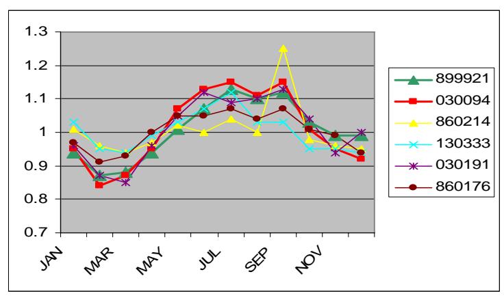
Figure 6.1 Seasonal Factors for the Test Site 899921 and the First Five Closest Matching Sites
Figure 6.2 plots the percentage differences in the MSFs of site 899921 and its matching sites. The curve labeled the average is based on the average MSFs of the first two best matching sites. Except for the second and third best matching sites, note good matches with site 899921. The percentage differences in MSFs for the first, third, and fifth sites are limited to a range of about -5% to +5%. The averages of the 12 month percentage differences for each of the matching sites are 0.036901, 0.070285, 0.062111, 0.028722, 0.043845, and 0.039484 for the first, second, third, fourth, fifth, and average, respectively. The fourth site is most similar to the test site. The first site and the average are also rather close.
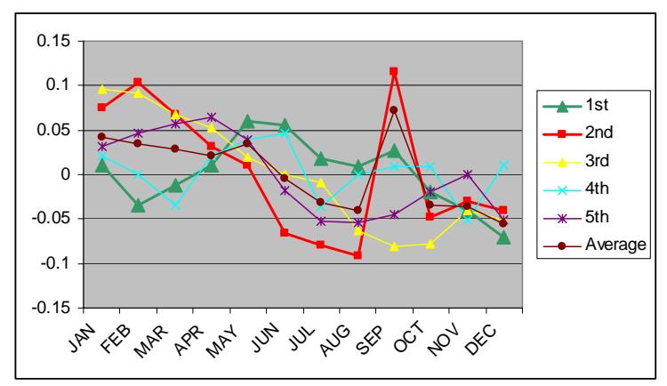
Figure 6.2 Percentage Difference in the MSFs for Site 899921 and the First Five Best Matches
### **6.3 MSF Assignment within Model Regions and Based on a Reduced Variable Set**
One concern regarding the above assignment method is that it involves too many variables. Some of these have relatively low R2 values. It is desirable that the number of variables be as small as possible. Because variables with low R2 values have small weighting factors, it may be possible to exclude them entirely from the assignment process. In the experiment described in this section, a reduced variable set is tested. For each of the three regions, the partial R2 values for each of the variables from the 12 regression models are summed. If a variable appears four times in the models for one region, for instance, the sum will contain four partial R2 values. If this sum of partial R2 is less than a certain value, the variable is not used for assignment purposes. For North and Central Florida, the variables are both reduced from 19 to 9 with a cutoff value of 0.2 for the sum of partial R2 values. For South Florida, the size of the variable set is reduced to 6 from 11 using a cutoff value of 0.15. Tables 6.7, 6.8, and 6.9 show the assignment results for the three regions, respectively.
The reduced variables used to calculate the similarity scores for sites in three model regions are summarized in Table 6.6*.*
Table 6.6 Reduced Variable Sets Used for Assignment for Three Model Regions
| District | Variables |
|----------|---------------------------------------------------------|
| North | FR, HotlP, MseumP, RETIRE, SHP, ST22, ST23, Rt_Low, and |
| | SU |
| Central | AgriP, CO, MA, MInc, PA, RETIRE, SHP, ST23, and Rt_Low |
| South | HotlP, MA, ManuP, MseumP, RETIRE, and SHP |
Table 6.7 Assignment for North Florida with Reduced Variables
| Test Sites | | | Best Matching Sites | | | |
|------------|--------|--------|---------------------|--------|--------|--|
| | 1st | 2nd | 3rd | 4th | 5th | |
| 260323 | 550208 | 550207 | 550300 | 710189 | 550226 | |
| 290286 | 729923 | 720161 | 509940 | 290320 | 720172 | |
| 550206 | 550300 | 550207 | 550208 | 550226 | 550212 | |
| 559908 | 260185 | 550212 | 550206 | 550300 | 550226 | |
| 720161 | 729923 | 290320 | 720172 | 290286 | 720171 | |
| 780329 | 720172 | 480282 | 480159 | 480156 | 570250 | |
| 550207 | 550226 | 550300 | 550208 | 550206 | 550209 | |
| 460315 | 530117 | 509940 | 360317 | 110246 | 570250 | |
| 530117 | 460315 | 360317 | 509940 | 110246 | 080283 | |
| 460308 | 740182 | 480156 | 360249 | 720121 | 570318 | |
| 080283 | 360317 | 730335 | 460315 | 530117 | 110246 | |
| 360264 | 460315 | 730335 | 360317 | 020044 | 530117 | |
| 110246 | 360317 | 780311 | 720172 | 509940 | 480282 | |
| 580261 | 570318 | 729923 | 480156 | 740182 | 360249 | |
| 729923 | 720161 | 290286 | 480156 | 780311 | 570318 | |
| 550212 | 559908 | 260185 | 550206 | 550226 | 550207 | |
| 730335 | 080283 | 020044 | 360264 | 360317 | 730292 | |
| 260185 | 559908 | 550212 | 550206 | 550226 | 550209 | |
| 730292 | 360317 | 080283 | 730335 | 489924 | 760105 | |
| 760105 | 360317 | 080283 | 730335 | 110246 | 509940 | |
| 290320 | 720161 | 729923 | 290286 | 720171 | 570318 | |
| 509940 | 780311 | 110246 | 460315 | 360249 | 480156 | |
| 550151 | 550304 | 550207 | 550226 | 550300 | 550208 | |
| 550208 | 550300 | 550207 | 550226 | 550206 | 550209 | |
| 550209 | 550226 | 550300 | 550207 | 260185 | 550208 | |
| 550213 | 550206 | 550300 | 550208 | 550207 | 550212 | |
| 550226 | 550207 | 550209 | 550300 | 550208 | 550206 | |
| 720062 | 720121 | 460308 | 570167 | 740182 | 480159 | |
| 720121 | 570167 | 720062 | 460308 | 480325 | 589937 | |
| 720172 | 570250 | 480282 | 480159 | 480156 | 360249 | |
| 720216 | 489924 | 460308 | 729914 | 480159 | 360249 | |
| 740182 | 460308 | 720109 | 360249 | 480156 | 570318 | |
| 780311 | 360249 | 480156 | 720172 | 480282 | 509940 | |
| 720109 | 740182 | 360249 | 589937 | 460308 | 480156 | |
| 720171 | 720161 | 729914 | 489924 | 290320 | 720216 | |
| | | | Best Matching Sites | | |
|------------|--------|--------|---------------------|--------|--------|
| Test Sites | 1st | 2nd | 3rd | 4th | 5th |
| 550300 | 550206 | 550207 | 550208 | 550226 | 550209 |
| 550304 | 720171 | 550207 | 550300 | 550208 | 550151 |
| 729914 | 489924 | 729923 | 720216 | 780311 | 480156 |
| 460166 | 570293 | 460305 | 760105 | 780329 | 290320 |
| 460305 | 290320 | 720161 | 720171 | 580261 | 729923 |
| 480159 | 360249 | 480156 | 720172 | 480282 | 570250 |
| 480282 | 720172 | 480159 | 570250 | 780311 | 110246 |
| 480325 | 570167 | 720121 | 589937 | 720109 | 360249 |
| 570250 | 720172 | 480282 | 480159 | 360249 | 480156 |
| 570293 | 290320 | 550151 | 720161 | 460305 | 720171 |
| 589937 | 720109 | 740182 | 480325 | 360249 | 720121 |
| 570318 | 480156 | 740182 | 360249 | 460308 | 480159 |
| 489924 | 720216 | 729914 | 720172 | 480156 | 570250 |
| 480156 | 360249 | 460308 | 480159 | 740182 | 570318 |
| 570167 | 720121 | 480325 | 460308 | 720062 | 480156 |
| 600168 | 760105 | 480282 | 570250 | 460308 | 480159 |
| 710189 | 720121 | 720062 | 480325 | 570167 | 260323 |
| 080294 | 110177 | 760105 | 360264 | 730335 | 020044 |
| 110177 | 080294 | 020044 | 360264 | 760105 | 730335 |
| 360249 | 480156 | 480159 | 780311 | 740182 | 720109 |
| 020044 | 730335 | 360317 | 080283 | 360264 | 760105 |
| 360317 | 110246 | 080283 | 460315 | 530117 | 509940 |
The variables used to calculate the similarity scores in Central Florida are *AgriP, CO, MA, MInc, PA, RETIRE, SHP, ST23*, and *Rt\_Low*. Four of these are the same as those for North Florida.
Table 6.8 TTMSs Assignment for Central Florida with Reduced Parameters
| | | | Best Matching Sites | | |
|------------|--------|--------|---------------------|--------|--------|
| Test Sites | 1st | 2nd | 3rd | 4th | 5th |
| 100106 | 100080 | 150183 | 750204 | 750196 | 109926 |
| 100321 | 100162 | 770102 | 750154 | 750038 | 140013 |
| 150302 | 750204 | 109922 | 100194 | 100224 | 109926 |
| 109922 | 100194 | 750204 | 109926 | 750196 | 100224 |
| 169927 | 140199 | 150295 | 700113 | 750038 | 100162 |
| 750038 | 700113 | 770102 | 150295 | 100162 | 750154 |
| 750175 | 100110 | 750196 | 109922 | 100123 | 100194 |
| 770197 | 140013 | 750038 | 700113 | 150295 | 750154 |
| 790133 | 100110 | 700284 | 100123 | 750175 | 750196 |
| 799929 | 790133 | 700284 | 979932 | 100123 | 100110 |
| 100080 | 150183 | 100123 | 750196 | 100110 | 100194 |
| 100110 | 750175 | 750196 | 100123 | 750204 | 109922 |
| 100123 | 750196 | 100110 | 109922 | 750175 | 100194 |
| 100194 | 109922 | 109926 | 750196 | 750204 | 100224 |
| | | | Best Matching Sites | | |
|------------|--------|--------|---------------------|--------|--------|
| Test Sites | 1st | 2nd | 3rd | 4th | 5th |
| 140013 | 770102 | 770197 | 750154 | 100162 | 750038 |
| 140190 | 750130 | 750204 | 100224 | 770343 | 109926 |
| 150086 | 750154 | 770102 | 140013 | 100162 | 920265 |
| 150183 | 100080 | 790133 | 160310 | 700284 | 100110 |
| 150295 | 700113 | 750038 | 750154 | 770197 | 100162 |
| 100224 | 109926 | 770343 | 109922 | 100194 | 750204 |
| 109926 | 100224 | 100194 | 109922 | 770343 | 750204 |
| 150066 | 150302 | 160310 | 700284 | 750175 | 100110 |
| 100162 | 100321 | 770102 | 750154 | 750038 | 140013 |
| 140199 | 150295 | 700113 | 169927 | 750038 | 770197 |
| 160275 | 799929 | 160310 | 790133 | 979932 | 169927 |
| 160128 | 100106 | 150183 | 100080 | 790133 | 100123 |
| 160310 | 150183 | 100080 | 150066 | 790133 | 979932 |
| 700113 | 750038 | 150295 | 100162 | 770102 | 770197 |
| 700114 | 150295 | 750038 | 140013 | 750154 | 770197 |
| 700284 | 790133 | 100110 | 770343 | 140190 | 750130 |
| 750130 | 140190 | 100224 | 770343 | 750204 | 109926 |
| 750154 | 770102 | 100162 | 100321 | 150086 | 750038 |
| 750196 | 100194 | 109922 | 100123 | 750175 | 100110 |
| 750204 | 109922 | 100194 | 109926 | 100224 | 750196 |
| 770102 | 100162 | 750154 | 100321 | 750038 | 140013 |
| 770343 | 109926 | 100224 | 750130 | 750204 | 109922 |
| 920265 | 150086 | 750154 | 100162 | 770102 | 100321 |
| 979932 | 100110 | 750175 | 790133 | 100123 | 750196 |
The variables used to calculate the similarity scores for the TTMSs in South Florida are *HotlP, MA, ManuP, MseumP, RETIRE,* and *SHP.* Four variables are the same as those for North Florida and three are the same as those for Central Florida*.* The *RETIRE* and *SHP* variables are common to all three regions.
Table 6.9 Assignment Results for South Florida with a Reduced Variable Set
| Test Sites | Best Matching Sites | | | | | | |
|------------|---------------------|--------|--------|--------|--------|--|--|
| | 1st | 2nd | 3rd | 4th | 5th | | |
| 170181 | 130180 | 979913 | 880314 | 890332 | 170225 | | |
| 030094 | 899921 | 860214 | 130333 | 030191 | 860176 | | |
| 860150 | 010228 | 030094 | 860306 | 899921 | 860214 | | |
| 860214 | 030094 | 899921 | 130333 | 010228 | 030191 | | |
| 860306 | 860214 | 030094 | 899921 | 860150 | 930010 | | |
| 870178 | 870266 | 870188 | 930257 | 870193 | 970267 | | |
| 870266 | 930257 | 870188 | 970267 | 979934 | 870178 | | |
| 930099 | 930101 | 940260 | 120203 | 970403 | 860186 | | |
| 970267 | 870266 | 979934 | 930257 | 970430 | 870188 | | |
| 970416 | 930174 | 970417 | 870108 | 890332 | 970410 | | |
| | Best Matching Sites | | | | |
|------------|---------------------|--------|--------|--------|--------|
| Test Sites | 1st | 2nd | 3rd | 4th | 5th |
| 979934 | 970267 | 870266 | 930257 | 870188 | 970430 |
| 890332 | 970417 | 880314 | 930174 | 979913 | 970416 |
| 970421 | 860163 | 880314 | 930198 | 970416 | 970410 |
| 930198 | 860331 | 930217 | 120184 | 040145 | 970421 |
| 870193 | 870188 | 870266 | 970430 | 870178 | 930257 |
| 120184 | 860176 | 930217 | 860331 | 930198 | 040145 |
| 010228 | 860214 | 030094 | 899921 | 860150 | 130333 |
| 040145 | 930217 | 860331 | 970417 | 930198 | 120184 |
| 170225 | 870108 | 940260 | 979913 | 979933 | 970403 |
| 130333 | 030191 | 860176 | 899921 | 120184 | 030094 |
| 130180 | 170181 | 979913 | 170225 | 870108 | 880314 |
| 030191 | 130333 | 860176 | 120184 | 930217 | 860331 |
| 120203 | 879930 | 860186 | 970403 | 940260 | 870187 |
| 860163 | 970421 | 970410 | 880314 | 860331 | 890332 |
| 860176 | 120184 | 030191 | 930217 | 130333 | 860331 |
| 860186 | 970403 | 940260 | 940334 | 860298 | 860222 |
| 860215 | 930087 | 010228 | 860214 | 030094 | 899921 |
| 860222 | 870187 | 979933 | 860298 | 860186 | 970403 |
| 860298 | 860222 | 979933 | 860186 | 970403 | 930101 |
| 860331 | 930217 | 040145 | 930198 | 120184 | 970416 |
| 870031 | 870108 | 930174 | 970416 | 970417 | 979913 |
| 870096 | 870187 | 860222 | 970267 | 979933 | 979934 |
| 870108 | 940334 | 170225 | 940260 | 970416 | 970403 |
| 870187 | 860222 | 979933 | 970430 | 860186 | 860298 |
| 870188 | 870266 | 930257 | 970267 | 870178 | 870193 |
| 870258 | 120203 | 940334 | 860186 | 970403 | 879930 |
| 879930 | 120203 | 860186 | 970403 | 870187 | 940260 |
| 930010 | 860176 | 120184 | 930217 | 930198 | 860331 |
| 930087 | 860215 | 010228 | 899921 | 860150 | 030094 |
| 930101 | 940260 | 930099 | 970403 | 860186 | 860298 |
| 930174 | 970416 | 970417 | 890332 | 880314 | 979913 |
| 930217 | 860331 | 040145 | 120184 | 930198 | 970417 |
| 930257 | 870266 | 870188 | 970267 | 979934 | 870178 |
| 970403 | 860186 | 940260 | 940334 | 930101 | 120203 |
| 970410 | 930174 | 979913 | 860163 | 970416 | 170225 |
| 970413 | 930198 | 120184 | 930217 | 860176 | 130333 |
| 970417 | 890332 | 930174 | 880314 | 970416 | 979913 |
| 970430 | 970267 | 870266 | 870193 | 870188 | 860222 |
| 979933 | 860222 | 860298 | 860186 | 870187 | 970403 |
| 880314 | 890332 | 970417 | 930174 | 970421 | 979913 |
| 880326 | 870188 | 870193 | 870178 | 870266 | 860222 |
| 890259 | 860215 | 930087 | 010228 | 860150 | 860306 |
| 899921 | 030094 | 860214 | 130333 | 030191 | 860176 |
| | Best Matching Sites | | | | | |
|------------|---------------------|--------|--------|--------|--------|--|
| Test Sites | 1st | 2nd | 3rd | 4th | 5th | |
| 940260 | 970403 | 860186 | 940334 | 930101 | 870108 | |
| 940334 | 970403 | 860186 | 940260 | 870108 | 860298 | |
| 979913 | 170181 | 890332 | 170225 | 130180 | 930174 | |
Compared to the assignment results obtained based on the full set of variables, 40 of 57 sites see the first best matching sites remain unchanged for North Florida. For Central Florida, the number of sites remaining unchanged is 25 out of 38. There are 46 of 56 sites remaining unchanged for South Florida. Coincidently, the assignment results for TTMS 899921, discussed in the preceding section, are exactly the same as before.
### **6.4 Assignment in Urban Areas within FDOT Districts and Based on a Reduced Variable Set**
In the SF assignment process, jurisdiction sometimes can be a consideration. In fact, in current practice, only nearby TTMSs within the same county or an FDOT district are used when determining the seasonal factors for a short-term count site. In this section, a geographic constraint is applied to test how such restrictions affect the assignment results. The geographic constraint is that the assignment is carried out with TTMSs within an FDOT district. County is not selected as the geographic unit for this purpose. This is because some counties have too few TTMSs to reflect a variety of land use conditions.
There are seven FDOT districts in Florida. The district boundaries and urban TTMS locations are illustrated in Figure 6.3. Note that the boundaries of the three model regions (see Figure 4.3) do not align with the district boundaries exactly.
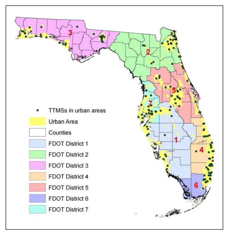
Figure 6.3 Boundaries of FDOT Districts
The variables used for assignment in each district are taken from the models of a region that has the most overlap with the district. For Districts 2 and 3, the variables are from the North Florida models. For Districts 5 and 7, the variables from the Central Florida models are applied. For Districts 1, 4, and 6, the variables from the South Florida models are adopted. Table 6.10 lists the variables used for each district. The assignment results are shown in Tables 6.11 through 6.17.
Table 6.10 Variable Sets Used for Assignment for Seven FDOT Districts
| District | Variables |
|----------|------------------------------------------------------------|
| 1, 4, 6 | HotlP, MA, ManuP, MseumP, RETIRE, and SHP |
| 2, 3 | FR, HotlP, MseumP, RETIRE, SHP, ST22, ST23, Rt_Low, and SU |
| 5, 7 | AgriP, CO, MA, MInc, PA, RETIRE, SHP, ST23, and Rt_Low |
Table 6.11 Assignment Results for District 1 with a Reduced Variable Set
| | Best Matching Sites | | | | |
|------------|---------------------|--------|--------|--------|--------|
| Test Sites | 1st | 2nd | 3rd | 4th | 5th |
| 010228 | 169927 | 160275 | 030094 | 160310 | 130333 |
| 030094 | 130333 | 030191 | 010228 | 120184 | 040145 |
| 030191 | 130333 | 120184 | 040145 | 030094 | 170181 |
| 040145 | 120184 | 030191 | 170181 | 130333 | 130180 |
| 120184 | 040145 | 030191 | 130333 | 170181 | 170225 |
| 120203 | 170225 | 160128 | 130180 | 170181 | 040145 |
| 170181 | 130180 | 170225 | 160128 | 040145 | 120203 |
| 170225 | 130180 | 170181 | 160128 | 120203 | 040145 |
| 160275 | 169927 | 010228 | 160310 | 030094 | 130333 |
| 130333 | 030191 | 120184 | 030094 | 040145 | 170181 |
| 130180 | 170181 | 170225 | 160128 | 040145 | 120203 |
| 160128 | 170225 | 130180 | 120203 | 170181 | 040145 |
| 160310 | 160275 | 010228 | 169927 | 030094 | 030191 |
| 169927 | 160275 | 010228 | 030094 | 160310 | 130333 |
Table 6.12 Assignment Results for District 2 with a Reduced Variable Set
| | | | Best Matching Sites | | |
|------------|--------|--------|---------------------|--------|--------|
| Test Sites | 1st | 2nd | 3rd | 4th | 5th |
| 260185 | 720172 | 720109 | 740182 | 780311 | 720062 |
| 260323 | 710189 | 720121 | 720062 | 740182 | 720109 |
| 290286 | 729923 | 720161 | 290320 | 720172 | 729914 |
| 290320 | 720161 | 729923 | 290286 | 720171 | 780311 |
| 720062 | 720121 | 740182 | 720109 | 720172 | 710189 |
| 720121 | 720062 | 720109 | 740182 | 710189 | 720172 |
| 720161 | 729923 | 290286 | 290320 | 720172 | 720171 |
| 720172 | 780311 | 720109 | 740182 | 260185 | 720062 |
| 720216 | 720109 | 729914 | 740182 | 720172 | 720062 |
| 729923 | 720161 | 290286 | 720172 | 780311 | 290320 |
| 740182 | 720109 | 720062 | 720172 | 720121 | 260185 |
| 760105 | 780311 | 720172 | 290286 | 740182 | 720109 |
| 780311 | 720172 | 720109 | 740182 | 260185 | 729923 |
| 780329 | 780311 | 720172 | 740182 | 720109 | 720062 |
| 720109 | 740182 | 720172 | 720121 | 720062 | 780311 |
| 720171 | 720161 | 729914 | 290320 | 729923 | 720216 |
| 710189 | 720121 | 720062 | 260323 | 720109 | 740182 |
| 729914 | 720216 | 729923 | 720171 | 290286 | 720172 |
Table 6.13 Assignment Results for District 3 with a Reduced Variable Set
| | | | Best Matching Sites | | |
|------------|--------|--------|---------------------|--------|--------|
| Test Sites | 1st | 2nd | 3rd | 4th | 5th |
| 460166 | 460305 | 570293 | 600168 | 580261 | 480282 |
| 460305 | 580261 | 570318 | 480156 | 460308 | 480159 |
| 460315 | 530117 | 509940 | 480282 | 570250 | 480159 |
| 480159 | 480156 | 570250 | 480282 | 460308 | 589937 |
| 480282 | 480159 | 570250 | 480156 | 509940 | 550209 |
| 480325 | 570167 | 589937 | 550208 | 480159 | 460308 |
| 509940 | 460315 | 530117 | 480282 | 570250 | 480156 |
| 530117 | 460315 | 509940 | 480282 | 570250 | 480159 |
| 550151 | 550207 | 550300 | 550226 | 559908 | 550206 |
| 550206 | 550300 | 550207 | 550208 | 559908 | 550226 |
| 550208 | 550300 | 550206 | 550207 | 550226 | 480325 |
| 550209 | 550226 | 550207 | 480282 | 550300 | 559908 |
| 550212 | 550207 | 550226 | 559908 | 550206 | 550300 |
| 550213 | 550206 | 550208 | 550300 | 550207 | 570167 |
| 550226 | 550207 | 550300 | 550209 | 559908 | 550206 |
| 559908 | 550206 | 550226 | 550300 | 550212 | 550207 |
| 570250 | 480159 | 480156 | 480282 | 460308 | 589937 |
| 570293 | 480282 | 550151 | 480156 | 480159 | 570250 |
| 580261 | 570318 | 480156 | 460308 | 570250 | 480159 |
| 589937 | 460308 | 570167 | 480159 | 480325 | 480156 |
| 570318 | 480156 | 460308 | 480159 | 580261 | 570250 |
| 489924 | 480156 | 480282 | 570250 | 480159 | 570318 |
| 460308 | 480156 | 570318 | 480159 | 589937 | 570167 |
| 480156 | 480159 | 570318 | 460308 | 570250 | 480282 |
| 550300 | 550206 | 550207 | 550208 | 550226 | 559908 |
| 570167 | 480325 | 589937 | 460308 | 480156 | 480159 |
| 600168 | 460308 | 570318 | 480156 | 460305 | 570250 |
| 550207 | 550226 | 550300 | 550206 | 550208 | 550212 |
| 550304 | 550300 | 550151 | 489924 | 550207 | 550206 |
Table 6.14 Assignment Results for District 4 with a Reduced Variable Set
| | Best Matching Sites | | | | | | | | | | |
|------------|---------------------|--------|--------|--------|--------|--|--|--|--|--|--|
| Test Sites | | | | | | | | | | | |
| | 1st | 2nd | 3rd | 4th | 5th | | | | | | |
| 860150 | 860306 | 899921 | 860214 | 930010 | 860176 | | | | | | |
| 860163 | 970421 | 970410 | 880314 | 860331 | 970416 | | | | | | |
| 860176 | 930217 | 860331 | 930198 | 930010 | 970413 | | | | | | |
| 860186 | 970403 | 940260 | 940334 | 860222 | 860298 | | | | | | |
| 860214 | 899921 | 860176 | 860306 | 930198 | 970413 | | | | | | |
| 860215 | 930087 | 860214 | 899921 | 860306 | 860150 | | | | | | |
| 860222 | 979933 | 860298 | 860186 | 970403 | 940334 | | | | | | |
| 860298 | 860222 | 979933 | 860186 | 970403 | 930101 | | | | | | |
| 860306 | 860214 | 899921 | 860150 | 930010 | 860176 | | | | | | |
| 860331 | 930217 | 930198 | 970416 | 860163 | 930174 | | | | | | |
| 880314 | 890332 | 970417 | 930174 | 970421 | 979913 | | | | | | |
| 880326 | 930257 | 860298 | 860222 | 979933 | 930101 | | | | | | |
| 890259 | 860215 | 930087 | 860306 | 860150 | 860214 | | | | | | |
| 890332 | 970417 | 880314 | 930174 | 979913 | 970416 | | | | | | |
| 899921 | 860214 | 860176 | 930198 | 970413 | 930217 | | | | | | |
| 930010 | 860176 | 930217 | 930198 | 860331 | 970413 | | | | | | |
| 930087 | 860215 | 899921 | 860150 | 860214 | 860306 | | | | | | |
| 930099 | 930101 | 940260 | 970403 | 860186 | 860298 | | | | | | |
| 930101 | 930099 | 940260 | 970403 | 860186 | 860298 | | | | | | |
| 930174 | 970416 | 970417 | 890332 | 880314 | 979913 | | | | | | |
| 930198 | 860331 | 930217 | 970421 | 880314 | 970413 | | | | | | |
| 930217 | 860331 | 930198 | 970417 | 860176 | 890332 | | | | | | |
| 930257 | 880326 | 860222 | 860298 | 930101 | 930099 | | | | | | |
| 940260 | 970403 | 860186 | 940334 | 930101 | 979933 | | | | | | |
| 940334 | 970403 | 860186 | 940260 | 860298 | 860222 | | | | | | |
| 970403 | 860186 | 940260 | 940334 | 930101 | 860222 | | | | | | |
| 970410 | 860163 | 930174 | 979913 | 970416 | 890332 | | | | | | |
| 970413 | 930198 | 930217 | 860176 | 860331 | 970421 | | | | | | |
| 970416 | 930174 | 970417 | 890332 | 970410 | 880314 | | | | | | |
| 970417 | 890332 | 930174 | 880314 | 970416 | 979913 | | | | | | |
| 970421 | 860163 | 880314 | 930198 | 970416 | 970410 | | | | | | |
| 979913 | 890332 | 930174 | 880314 | 970417 | 970410 | | | | | | |
| 979933 | 860222 | 860298 | 860186 | 970403 | 940334 | | | | | | |
Table 6.15 Assignment Results for District 5 with a Reduced Variable Set
| | | | Best Matching Sites | | |
|------------|--------|--------|---------------------|--------|--------|
| Test Sites | 1st | 2nd | 3rd | 4th | 5th |
| 110177 | 799929 | 360264 | 920265 | 700113 | 730335 |
| 700113 | 750038 | 770102 | 770197 | 750154 | 360264 |
| 700114 | 750038 | 750154 | 700113 | 360317 | 770197 |
| 730292 | 360317 | 730335 | 790133 | 700284 | 799929 |
| 730335 | 790133 | 799929 | 700284 | 979932 | 730292 |
| 750038 | 700113 | 770102 | 750154 | 770197 | 360264 |
| 750130 | 750204 | 770343 | 750196 | 750175 | 790133 |
| 750154 | 770102 | 750038 | 770197 | 700113 | 920265 |
| 750175 | 750196 | 750204 | 770343 | 750130 | 979932 |
| 750196 | 750175 | 750204 | 770343 | 750130 | 790133 |
| 750204 | 750130 | 750196 | 770343 | 750175 | 790133 |
| 770102 | 750154 | 750038 | 700113 | 770197 | 750196 |
| 770197 | 750038 | 770102 | 750154 | 700113 | 360264 |
| 770343 | 750196 | 750204 | 750130 | 750175 | 790133 |
| 790133 | 730335 | 979932 | 700284 | 750204 | 750196 |
| 799929 | 730335 | 790133 | 700284 | 110177 | 979932 |
| 920265 | 750154 | 770102 | 750038 | 700113 | 770197 |
| 979932 | 790133 | 750175 | 750196 | 750204 | 750130 |
| 110246 | 360249 | 790133 | 770343 | 360317 | 750204 |
| 360249 | 750196 | 750204 | 750175 | 110246 | 770343 |
| 360264 | 700113 | 750038 | 770197 | 770102 | 750154 |
| 700284 | 790133 | 730335 | 750130 | 750204 | 770343 |
| 360317 | 730292 | 790133 | 730335 | 110246 | 750196 |
Table 6.16 Assignment Results for District 6 with a Reduced Variable Set
| Test Sites | | | Best Matching Sites | | |
|------------|--------|--------|---------------------|--------|--------|
| | 1st | 2nd | 3rd | 4th | 5th |
| 870031 | 870108 | 870258 | 879930 | 970430 | 870187 |
| 870096 | 870193 | 970267 | 870266 | 870187 | 870188 |
| 870108 | 870031 | 870258 | 879930 | 870187 | 970430 |
| 870178 | 870266 | 870188 | 979934 | 970267 | 900164 |
| 870187 | 970430 | 870193 | 870096 | 970267 | 870266 |
| 870188 | 870266 | 979934 | 970267 | 870178 | 900164 |
| 870193 | 970267 | 870188 | 970430 | 870096 | 870266 |
| 870258 | 879930 | 970430 | 870187 | 870193 | 870108 |
| 870266 | 870188 | 979934 | 970267 | 870178 | 900164 |
| 879930 | 870258 | 870187 | 970430 | 970267 | 870193 |
| 900164 | 900165 | 900227 | 979934 | 870266 | 870188 |
| 900165 | 900164 | 900227 | 979934 | 870266 | 870188 |
| 900227 | 900164 | 900165 | 979934 | 870266 | 870188 |
| 970267 | 870266 | 870188 | 979934 | 870193 | 870178 |
| 970430 | 870187 | 870193 | 970267 | 870188 | 870266 |
| 979934 | 870266 | 870188 | 970267 | 900164 | 900165 |
Table 6.17 Assignment Results for District 7 with a Reduced Variable Set
| | | | Best Matching Sites | | |
|------------|--------|--------|---------------------|--------|--------|
| Test Sites | 1st | 2nd | 3rd | 4th | 5th |
| 080283 | 140199 | 150295 | 100162 | 100321 | 140013 |
| 080294 | 140199 | 080283 | 150295 | 020044 | 150086 |
| 100080 | 150183 | 100123 | 100110 | 100194 | 109922 |
| 100106 | 150183 | 100080 | 109926 | 100224 | 100194 |
| 100110 | 100123 | 109922 | 100194 | 109926 | 100224 |
| 100123 | 100110 | 109922 | 100194 | 109926 | 100224 |
| 100194 | 109922 | 109926 | 100224 | 100123 | 100110 |
| 100321 | 100162 | 140013 | 150086 | 150295 | 080283 |
| 140013 | 100162 | 150086 | 100321 | 150295 | 080283 |
| 140190 | 100224 | 109922 | 109926 | 100194 | 100110 |
| 150086 | 140013 | 100162 | 100321 | 150295 | 140199 |
| 150183 | 100080 | 100110 | 100123 | 100194 | 109922 |
| 150295 | 080283 | 100162 | 140013 | 140199 | 100321 |
| 150302 | 109922 | 100194 | 100224 | 109926 | 100123 |
| 020044 | 100110 | 100123 | 109922 | 140190 | 100224 |
| 100224 | 109926 | 100194 | 109922 | 140190 | 100110 |
| 109926 | 100224 | 100194 | 109922 | 100110 | 140190 |
| 150066 | 150302 | 100110 | 140190 | 100123 | 109922 |
| 100162 | 100321 | 140013 | 150086 | 150295 | 080283 |
| 109922 | 100194 | 109926 | 100224 | 100123 | 100110 |
| 140199 | 080283 | 150295 | 080294 | 100162 | 100321 |
The assignment results are examined to determine if they are reasonable. As an example, the assignment results for site 899921 are given below in Table 6.18. This table shows the effect of assignment based on district boundaries. It also shows the monthly seasonal factors of site 899921 and the matching TTMSs. The percentage difference between the MSFs of the test site and the matching TTMSs are also calculated. The MSFs and the percentage differences in the MSFs are averaged for the first two best matches and are shown in the last two rows of the table. The monthly seasonal factors of the matching TTMSs are plotted in Figure 6.4. The percentage differences between the MSFs of site 899921 and the matching TTMSs are also calculated and plotted in Figure 6.5.
Table 6.18 MSFs for Test Site 899921 and the First Five Best Matching Sites in District 4
| | Site | JAN | FEB | MAR | APR | MAY | JUN | JUL | AUG | SEP | OCT | NOV | DEC |
|-----------|--------|------|------|------|------|------|------|------|------|------|------|------|------|
| Test Site | 899921 | 0.94 | 0.87 | 0.88 | 0.94 | 1.01 | 1.07 | 1.13 | 1.10 | 1.12 | 1.03 | 0.99 | 0.99 |
| 1st best | 860214 | 1.01 | 0.96 | 0.94 | 0.97 | 1.02 | 1.00 | 1.04 | 1.00 | 1.25 | 0.98 | 0.96 | 0.95 |
| | | 7% | 10% | 7% | 3% | 1% | -7% | -8% | -9% | 12% | -5% | -3% | -4% |
| 2nd best | 860176 | 0.97 | 0.91 | 0.93 | 1.00 | 1.05 | 1.05 | 1.07 | 1.04 | 1.07 | 1.01 | 0.99 | 0.94 |
| | | 3% | 5% | 6% | 6% | 4% | -2% | -5% | -5% | -4% | -2% | 0% | -5% |
| 3rd best | | 1.00 | 0.95 | 0.94 | 0.97 | 1.01 | 1.03 | 1.04 | 1.01 | 1.05 | 1.01 | 1.00 | 0.99 |
| | 930198 | 6% | 9% | 7% | 3% | 0% | -4% | -8% | -8% | -6% | -2% | 1% | 0% |
| 4th best | 970413 | 1.01 | 0.94 | 0.92 | 1.00 | 1.03 | 1.05 | 1.05 | 1.02 | 1.10 | 1.04 | 0.93 | 0.94 |
| | | 7% | 8% | 5% | 6% | 2% | -2% | -7% | -7% | -2% | 1% | -6% | -5% |
| 5th best | 930217 | 1.01 | 0.96 | 0.94 | 0.98 | 1.01 | 1.03 | 1.03 | 1.01 | 1.09 | 1.02 | 0.98 | 0.96 |
| | | 7% | 10% | 7% | 4% | 0% | -4% | -9% | -8% | -3% | -1% | -1% | -3% |
| | | 0.99 | 0.94 | 0.94 | 0.99 | 1.04 | 1.03 | 1.06 | 1.02 | 1.16 | 1.00 | 0.98 | 0.95 |
| Average | | 5% | 7% | 6% | 5% | 2% | -4% | -7% | -7% | 4% | -3% | -2% | -5% |
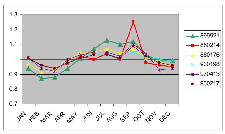
Figure 6.4 MSFs for the TTMS 899921 and the First Five Best Matching Sites within District 4
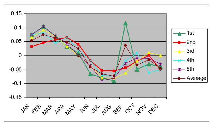
Figure 6.5 Percentage Differences between MSFs for Site 899921 and the First Five Best Matches within District 4
In this particular example, the three previous best matches (TTMSs 030094, 130333, and 030191) are not in the same district. As a result, the previous second and fifth best matches become the first and the second best within District 4. The average of the 12 month percentage differences for each of the matches becomes 0.070285, 0.043845, 0.055541, 0.05465, and 0.058067 for the first, second, third, fourth, and fifth best matches, respectively. The average of the scores of these matches is 0.051162. The differences have increased, indicating less accurate assignment results.
### **6.5 Evaluation of the Three Assignment Strategies**
The preceding sections described three assignment strategies. The question then naturally arises: Which strategy works best? This question cannot be answered based on the analysis of the lone test case shown here. To give an overall assessment of all of the test TTMSs, the average error is computed as follows for each assignment strategy:
These average errors reflect the average difference between the estimated MSFs and true MSFs for all tested sites within the same region.
Table 6.19 Average Errors of the Assignment Results Based on Full Variable Set
| Best Match | North | Central | South |
|------------|----------|----------|----------|
| 1st | 0.058453 | 0.053952 | 0.043630 |
| 2nd | 0.058136 | 0.042621 | 0.050254 |
| 3rd | 0.060341 | 0.045074 | 0.047321 |
| 4th | 0.058639 | 0.045981 | 0.046396 |
| 5th | 0.055406 | 0.049464 | 0.045786 |
| Average | 0.052953 | 0.042357 | 0.041964 |
It is clear from the above table that it is not necessarily true that the first best match is always better than others. However, the first best matches in South Florida appear to perform better than the second through the fifth. The second best matches in Central Florida are better than the other four. Note that the average of the first two best matches is always better overall than all of the others, as indicated by the last row in Table 6.19.
Table 6.20 shows the average errors in MSFs that are computed based on the reduced variable sets. They are not necessarily worse than those obtained using the full variable sets. Some errors, such as those for the first best matches in North and Central Florida, are even smaller than those derived using the full variable sets. This suggests that the reduced variable sets may potentially be used for assignment purposes.
Table 6.20 Average Errors of the Assignment Results Based on a Reduced Variable Set
| Best Match | North | Central | South |
|------------|----------|----------|----------|
| 1st | 0.057524 | 0.04345 | 0.046393 |
| 2nd | 0.063766 | 0.044593 | 0.050264 |
| 3rd | 0.058141 | 0.048900 | 0.04757 |
| 4th | 0.061914 | 0.053314 | 0.048486 |
| 5th | 0.064822 | 0.05012 | 0.046241 |
| Average | 0.053392 | 0.038877 | 0.043145 |
Table 6.21 gives the errors computed based on the results of assignment restricted to FDOT districts and using a reduced variable set. The first two best matches always give better overall performance. Compared with the errors associated with the strategy of region-wide assignment with a reduced variable set, it appears that the overall performance of the district based assignment method is slightly better for District 2 (North Florida) and District 4 (South Florida). That for other districts, however, has become worse. Still, the absolute values are not significantly different from those derived using the previous strategy.
Table 6.21 Average Errors of the Assignment Results Based on a Reduced Variable Set within a District
| Best Match | District1 | District2 | District3 | District4 | District5 | District6 | District7 |
|------------|-----------|-----------|-----------|-----------|-----------|-----------|-----------|
| 1st | 0.055805 | 0.047023 | 0.063454 | 0.045211 | 0.039331 | 0.04792 | 0.044181 |
| 2nd | 0.045057 | 0.048264 | 0.064206 | 0.044534 | 0.051907 | 0.049549 | 0.046537 |
| 3rd | 0.056179 | 0.058785 | 0.063131 | 0.045999 | 0.051234 | 0.047518 | 0.049129 |
| 4th | 0.062670 | 0.045114 | 0.059959 | 0.043438 | 0.057104 | 0.048628 | 0.045162 |
| 5th | 0.064921 | 0.049712 | 0.074597 | 0.046234 | 0.062475 | 0.059978 | 0.045482 |
| Average | 0.045502 | 0.043080 | 0.056779 | 0.039321 | 0.039919 | 0.044181 | 0.039135 |
### **7. CONCLUSIONS AND RECOMMENDATIONS**
In this research, a statewide study was conducted involving imputation of TTMS data, clustering of TTMSs to create seasonal factor groups, conducting regression analysis to identify influential land use variables that may affect seasonal factors, and a preliminary study of possible assignment methods.
Imputation refers to the replacement of missing data with a substitute that allows data analysis to be conducted without being misleading. Because less than 300 TTMSs are in service and 24.2% of them have missing data in 2000, imputation is necessary. The advantage of the imputation method adopted in this study is that it is easily understood and implemented. The disadvantage of this method is that it is time-consuming because manual adjustments have to be made for each site. This process, however, may be made more efficient through automation.
Cluster analysis has been applied to statewide TTMSs to create seasonal factor groups. A modelbased cluster technique using only the 12 MSFs has proven to be more practical in this regard. It also produced reasonable results. Variables that represent locations of TTMSs were also tested. However, they resulted in a large number of groups, with many groups consisting of a single TTMS.
Regression models were developed to identify influential variables for the seasonal factors of TTMSs. It was found that influential variables for the seasonal factors of the TTMSs are different in urban and rural areas and in different climate zones. To account for differences in climate, the urban areas are divided into three regions: North, Central, and South Florida. For North Florida, the most influential variables are found to be proximity of a TTMS to an urban freeway; employment related to hotels, camps, museums, art galleries, and gardens; retired households; seasonal households; population ages 11-13 and 14-17; retired households with low income; residential university; etc. For Central Florida, important variables are agriculture workers; proximity of a TTMS to an urban collector, minor arterial, or principal arterial; median household income; retired households; seasonal households; population ages 14-17; low-income retired households; proximity to a large residential university; etc*.* For South Florida, hotels, museums, manufacturing-related employment, retired and seasonal households, and proximity to principal arterials are significant variables.
The approach for modeling urban area TTMSs cannot be applied to rural TTMSs. This is because there is an insufficient number of TTMSs in which to divide rural areas to model them separately. An alternative approach was developed to separately model those TTMSs for which the hourly traffic pattern on a typical weekday shows a single peak (i.e., recreational travel dominates) and those for which the weekday hourly traffic pattern has a double peak (i.e., commute travel dominates). The models were improved as a result, particularly for the singlepeak TTMSs. These are more difficult to model due to the low land use intensity and through traffic. Hence, this improvement may be attributed to the intrinsic connection between daily traffic patterns and land use variables. These, in turn, are connected to the seasonal traffic variations. The more noticeable improvement in the models for the single-peak group may be because recreational roadways (single-peak pattern) have more seasonal variations, while the traffic on commuting roadways (double-peak pattern) varies less seasonally.
Some variables are significant regardless whether the TTMSs' hourly traffic patterns show a single or double peak. These include the distance to and population of a nearby urban area, seasonal households in South Florida, and retail employees in South Florida. For TTMSs with a single peak, manufacturing employment, a truck factor, population ages 18-64, and proximity to a freeway interchange were also found to be important. For the double-peak TTMSs, the distance from a TTMS to the closest public beach is found to be important. Several variables describe the spatial proximity to nearby urban areas and roadway function classes. The significance of these variables suggests that the basis for current practices considering the function class and roadway use may be valid in rural areas.
The influential variables obtained from the urban models were used in developing a method to identify a TTMS that is similar to a given count station in terms of its land uses or functions. A similarity score was developed to measure the similarity between two count sites. This score was based on the identified influential variables, which were weighted by their partial R2 values in the models. This approach showed promising results: The average of standard errors among estimated seasonal factors was about 5% overall.
The assignment method developed in this study offers at least three advantages. First, no additional TTMSs are required to validate the assignment results. This makes this approach more practical and less expensive when compared to, for example, a fuzzy decision tree. Second, a count site may be linked to multiple TTMSs. This provides the analyst with alternative TTMSs in case there is a sufficient basis to reject the best matching TTMS based on the selected variables. Third, this method can be tested with the same TTMSs that are used in the regression analysis. Although this is not to say that there is no need for independent testing using an entirely different set of data, this method allows the development of some understanding of how well the method works. Finally, this method has the potential to eliminate the need to conduct seasonal factor grouping.
To further develop the results from this study for implementation, the following research efforts are recommended.
- 1) Conduct more detailed analysis of the results of the assignment method to evaluate its accuracy. This involves determining the distribution of the errors, including the ranges, in addition to the currently used aggregate measure of mean errors. Understanding the locations or the characteristics of TTMSs where large errors occur will help identify variables that may be inappropriate. It will also indicate the need for additional variables, if any.
- 2) Apply the proposed assignment method to the assignment of seasonal factors in rural areas. Depending on the results, there may be a need to improve the regression models by identifying additional variables or to revise the definitions of existing variables.
- 3) Investigate the effect of inclusion or exclusion of different variables. This is especially true for some of the variables that are correlated with others, even though they are not included in the same equations. For instance, if the exclusion of a variable does not
change the assignment results, this variable may be left out to simplify the problem. Conversely, if a variable improves assignment results, it may be included even if its partial R2 from regression analysis may be low. The effectiveness of the weighting scheme and alternative weighting schemes may also be examined to improve the assignment results.
- 4) Explore the feasibility of estimating the seasonal factor for a given PTMS for each month based on those of one or more TTMSs that share similarities on a monthly basis, as opposed to matching a PTMS to a TTMS and borrowing all of the monthly seasonal factors from that TTMS.
- 5) Compare the assignment results from the proposed approach to those obtained using the existing method. In the existing method the average of seasonal factors of a TTMS group is assigned to a coverage count site.
- 6) Independently test the assignment methods by using data collected monthly from selected sites that are different from the existing TTMSs in terms of geographic location and land use and roadway characteristics. This testing serves two purposes. One is to validate the proposed assignment methods. The other is to investigate the distribution of existing TTMSs to determine whether they provide adequate coverage by representing a wide range, commonly encountered combinations of land uses and roadway types. In the assignment process, redundant TTMSs may be identified if many in relative spatial proximity are found to be similar to nearby PTMSs in both their land use and roadway characteristics and in their seasonal factors. Conversely, an area may also be identified as needing additional TTMSs because of their unique land use and roadway functions. To remove redundant TTMSs will reduce the operating and maintenance costs. The saved resources may be reinvested by adding TTMSs to needed areas to improve the accuracy of AADT estimation.
There are many opportunities to improve the efficiency of the entire process. Tasks that may be made highly automated include TTMS data imputation, investigation of abnormal data, variable compilation, regression analysis, and seasonal factor assignment. Finally, to benefit from the research results, a computer application needs to be created. This application should be GIS based, with a user-friendly interface.
### **REFERENCES**
FDOT (2002). *Project Traffic Forecasting Handbook*, Draft, Florida Department of Transportation, Tallahassee, FloridaFL.
HCM (2000). *Highway Capacity Manual 2000***,** Transportation Research Board, National Research Council, Washington, D.C.
Li, M.-T., F. Zhao, and L.-F. Chow (2006). *Assignment of Seasonal Factor Categories to Urban Coverage Count Stations Using a Fuzzy Decision Tree*, *ASCE Journal of Transportation Engineering*, Vol. 132, No. 8, 2006, pp. 654-662.
Sharma, S.C. (1983). *Improved Classification of Canadian Primary Highways According to Type of Road Use, Canadian Journal of Civil Engineering*, No. 3, Vol. 10, pp. 497-509.
Sharma, S.C., P.J. Lingras, M.U. Hassan, and N.A.S. Murthy (1986). *Road Classification According to Driver Population, Transportation Research Record 1090*, Transportation Research Board, National Research Council, Washington, D.C., pp. 61-69.
USDOT (2001). *Traffic Monitoring Guide*, Office of Highway Policy Information, Federal Highway Administration, U.S. Department of Transportation, Washington, D.C.
Zhao, F. and S. Chung (2001) *Contributing Factors of Annual Average Daily Traffic in a Florida County,* Transportation Research Record 1769, Transportation Research Board, National Research Council, Washington D.C., 2001, pp 113-122.
Zhao, F., M.-T. Li, and L.-F. Chow (2004). *Alternatives for Estimating Seasonal Factors on Rural and Urban Roads In Florida*. Final Report for Project BD015-03, Research Office, Florida Department of Transportation, Tallahassee, Florida.
### **APPENDIX A. IMPUTATION OF MSFS FOR URBAN AREA**
In this appendix, the data used for imputation and imputation results for the 26 TTMSs are presented. The content of the table and the profiles have been explained in Section 2.2.
### **A.1 Imputation for Site 979934**
| | JAN | FEB | MAR | APR | MAY | JUN | JUL | AUG | SEP | OCT | NOV | DEC |
|------------|------|------|------|------|------|------|------|-----------|------|------|------|------|
| 1997 | 1.03 | 0.99 | 0.97 | 1 | 1.01 | 1 | 1 | 0.98 | 1.02 | 0.99 | 1 | 1.02 |
| 1998 | 1.07 | 1 | 0.96 | 0.98 | 1.02 | 1 | 1.03 | 1.07 | 1.08 | 1 | 1 | 0.97 |
| 1999 | 0 | 0 | 0 | 0 | 0 | 0 | 0 | 0 | 0 | 0 | 1.04 | 1.01 |
| 2000 | | | | | | | | | | | | |
| 2001 | 0 | 0 | 0 | 0 | 0 | 0 | 0 | 0 | 0 | 0 | 0 | 0 |
| 2002 | 0 | 0 | 0 | 0 | 1.05 | 0.99 | 0 | 1 | 0 | 0.98 | 0.99 | 0.99 |
| 2003 | 1.09 | 1.02 | 0.99 | 1 | 1 | 0.99 | 0.99 | 0.97 | 0.98 | 0.94 | 1.18 | 0.98 |
| 2004 | 1.05 | 0.98 | 0.96 | 0.99 | 1 | 0.99 | 1 | 1 | 1.09 | 0.98 | 0.97 | 0.98 |
| 2005 | 1.02 | 0.98 | 0.95 | 0.96 | 0.98 | 1 | 1 | 0.99 | 1.06 | 1.12 | 1 | 0.98 |
| | | | | | | | | | | | | |
| 2000 | 0 | 0 | 0 | 0 | 0 | 0 | 0 | 0 | 0 | 0 | 0 | 0 |
| Imputation | 1.07 | 1 | 0.96 | 0.98 | 1.02 | 1 | 1.03 | 0.99 | 1.08 | 1 | 1 | 0.97 |
| Source | 1998 | 1998 | 1998 | 1998 | 1998 | 1998 | 1998 | Avg
98 | 1998 | 1998 | 1998 | 1998 |
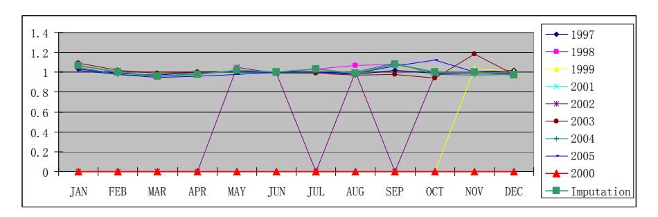
### **A.2 Imputation for Site 979913**
| | JAN | FEB | MAR | APR | MAY | JUN | JUL | AUG | SEP | OCT | NOV | DEC |
|------------|------|------|------|------|------|------|------|------|------|------|------|------|
| 1997 | 1.03 | 0.99 | 0.92 | 0.98 | 1 | 1.03 | 0.98 | 0.99 | 1.16 | 1.1 | 0.96 | 0.92 |
| 1998 | 1.03 | 1.01 | 0.99 | 0.96 | 1.03 | 1.06 | 0.96 | 0.99 | 1.07 | 1.07 | 0.96 | 0.9 |
| 1999 | 1.06 | 0.99 | 0.93 | 0.96 | 1.01 | 1.04 | 0.99 | 1 | 1.1 | 1.1 | 0.93 | 0.95 |
| 2000 | 0.87 | 0 | 0 | 0 | 1.01 | 1.08 | 0 | 0 | 0 | 1.07 | 0.98 | 0.96 |
| 2001 | 1.08 | 1.04 | 0.97 | 0.97 | 1.03 | 1.05 | 1 | 1.01 | 1.02 | 1.03 | 0.94 | 0.91 |
| 2002 | 1.07 | 1.02 | 0.92 | 1 | 1.03 | 0 | 0 | 0 | 1.13 | 1.05 | 0.98 | 0.89 |
| 2003 | 1.09 | 1.02 | 0.95 | 0 | 0 | 0 | 0 | 0.94 | 1.13 | 1.01 | 0.99 | 0.88 |
| 2004 | 1.07 | 1.03 | 0.98 | 0.97 | 1.01 | 1.04 | 0.98 | 1.04 | 1.15 | 1.06 | 0.88 | 0.93 |
| 2005 | 1.04 | 1.03 | 0.91 | 1.02 | 1 | 1.02 | 0.98 | 0 | 0 | 0 | 0 | 0 |
| | | | | | | | | | | | | |
| 2000 | 0.87 | 0 | 0 | 0 | 1.01 | 1.08 | 0 | 0 | 0 | 1.07 | 0.98 | 0.96 |
| Imputation | 1.06 | 0.99 | 0.93 | 0.96 | 1.01 | 1.04 | 0.99 | 1 | 1.1 | 1.1 | 0.93 | 0.95 |
| Source | 1999 | 1999 | 1999 | 1999 | 1999 | 1999 | 1999 | 1999 | 1999 | 1999 | 1999 | 1999 |
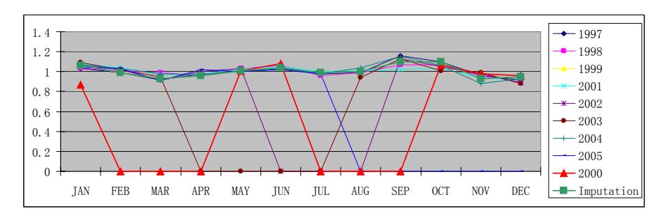
### **A.3 Imputation for Site 970413**
| | JAN | FEB | MAR | APR | MAY | JUN | JUL | AUG | SEP | OCT | NOV | DEC |
|------------|------|------|------|------|------|------|------|------|------|------|------|------|
| 1997 | 1.01 | 0.92 | 0.88 | 0.97 | 1.03 | 1.06 | 1.05 | 1.01 | 1.08 | 0 | 0 | 0 |
| 1998 | 1.01 | 0.95 | 0.94 | 0.94 | 1.03 | 1.05 | 1.05 | 1.03 | 1.08 | 1.03 | 0.98 | 0.94 |
| 1999 | 1.01 | 0.94 | 0.92 | 1 | 1.03 | 1.05 | 1.05 | 1.02 | 1.1 | 1.04 | 0.93 | 0.94 |
| 2000 | 1.03 | 0.95 | 0.93 | 0.97 | 1.01 | 1.04 | 1.09 | 0 | 0 | 0 | 0 | 0 |
| 2001 | 1.08 | 0.98 | 0.95 | 0.97 | 1.03 | 1.03 | 1.03 | 1 | 1.09 | 1.02 | 0.95 | 0.91 |
| 2002 | 1.07 | 0.98 | 0.91 | 1 | 1.02 | 1.02 | 1.02 | 1.01 | 1.08 | 1 | 0.95 | 0.94 |
| 2003 | 1.04 | 0.98 | 0.94 | 0.98 | 1.02 | 1.02 | 1.03 | 1 | 1.07 | 1 | 0.97 | 0.95 |
| 2004 | 1 | 0.94 | 0.93 | 0.96 | 1.02 | 1.04 | 1.03 | 1.02 | 1.09 | 0.99 | 0.97 | 0.95 |
| 2005 | | | | | | | | | | | | |
| | | | | | | | | | | | | |
| 2000 | 1.03 | 0.95 | 0.93 | 0.97 | 1.01 | 1.04 | 1.09 | 0 | 0 | 0 | 0 | 0 |
| Imputation | 1.01 | 0.94 | 0.92 | 1 | 1.03 | 1.05 | 1.05 | 1.02 | 1.1 | 1.04 | 0.93 | 0.94 |
| Source | 1999 | 1999 | 1999 | 1999 | 1999 | 1999 | 1999 | 1999 | 1999 | 1999 | 1999 | 1999 |
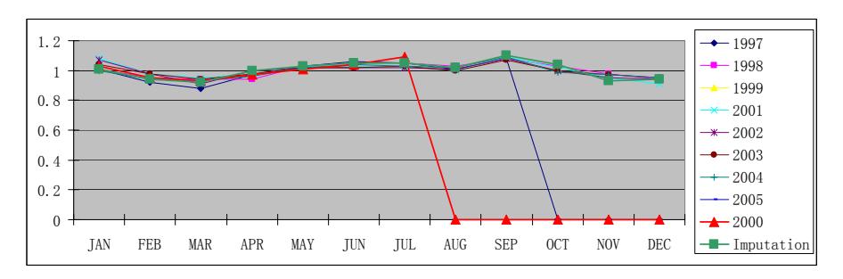
### **A.4 Imputation for Site 970410**
| | JAN | FEB | MAR | APR | MAY | JUN | JUL | AUG | SEP | OCT | NOV | DEC |
|------------|------|------|------|------|------|------|------|------|-------|-------|---------|------|
| 1997 | 1.04 | 0.94 | 0.92 | 0.98 | 1.04 | 1.07 | 1.07 | 1.03 | 1.08 | 1 | 0.95 | 0.92 |
| 1998 | 1.01 | 0.94 | 0.94 | 0.95 | 1.03 | 1.05 | 1.07 | 1.04 | 1.05 | 1.02 | 0.98 | 0.93 |
| 1999 | 1.01 | 0.94 | 0.93 | 0.99 | 1.04 | 1.04 | 1.06 | 1.01 | 1.13 | 1.13 | 0.93 | 0.93 |
| 2000 | 1.03 | 0.97 | 0.94 | 0.98 | 1.04 | 1.05 | 1.14 | 0 | 0 | 0 | 0 | 0.94 |
| 2001 | 1.04 | 0.95 | 0.94 | 0.97 | 1.04 | 1.03 | 1.04 | 1 | 1.09 | 1.02 | 0.97 | 0.94 |
| 2002 | 1.07 | 0.99 | 0.94 | 1.01 | 0 | 0 | 0 | 0 | 0 | 0 | 0 | 0 |
| 2003 | 0 | 0 | 0 | 0 | 0 | 0 | 0 | 0 | 0 | 0 | 0 | 0 |
| 2004 | | | | | | | | | | | | |
| 2005 | | | | | | | | | | | | |
| | | | | | | | | | | | | |
| 2000 | 1.03 | 0.97 | 0.94 | 0.98 | 1.04 | 1.05 | 1.14 | 0 | 0 | 0 | 0 | 0.94 |
| Imputation | 1.01 | 0.94 | 0.93 | 0.99 | 1.04 | 1.04 | 1.06 | 1.01 | 1.09 | 1.01 | 0.96 | 0.93 |
| | | | | | | | | | Avg - | Avg - | | |
| Source | 1999 | 1999 | 1999 | 1999 | 1999 | 1999 | 1999 | 1999 | 99 | 99 | Avg all | 1999 |
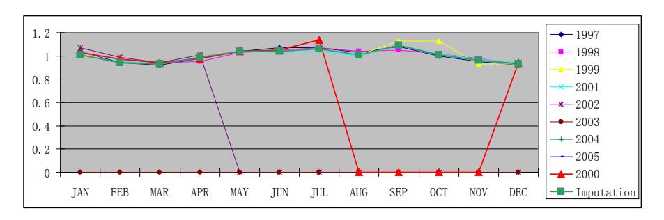
### **A.5 Imputation for Site 970403**
| | JAN | FEB | MAR | APR | MAY | JUN | JUL | AUG | SEP | OCT | NOV | DEC |
|------------|------|------|------|------|------|------|------|------|------|------|------|------|
| 1997 | 1.07 | 1 | 0.97 | 1 | 1.05 | 1.01 | 1.06 | 0.98 | 1 | 0.92 | 0.97 | 0.98 |
| 1998 | 1.04 | 0.99 | 0.96 | 0.97 | 1.01 | 1 | 1.03 | 1 | 1.03 | 0.99 | 1 | 0.98 |
| 1999 | 1.05 | 1.01 | 1 | 1 | 1.02 | 1 | 1.03 | 0.99 | 1.03 | 1 | 0.95 | 0.93 |
| 2000 | 0 | 0 | 0 | 0 | 0 | 0 | 0 | 0 | 0 | 0 | 0 | 0 |
| 2001 | 0 | 0 | 0 | 0 | 0 | 0 | 0 | 0.95 | 1.05 | 1 | 1.01 | 0.99 |
| 2002 | 1.08 | 1.01 | 0.98 | 0.99 | 1.01 | 1.01 | 1.02 | 0.98 | 1.02 | 0.96 | 0.96 | 0.96 |
| 2003 | 1.08 | 1.01 | 0.99 | 1.01 | 1.02 | 1.01 | 1.01 | 0.99 | 0.99 | 0.95 | 0.98 | 0.98 |
| 2004 | 1.04 | 0.97 | 0.98 | 1 | 1.01 | 1.02 | 1.02 | 1.02 | 0.99 | 0.98 | 0.99 | 0.99 |
| 2005 | 0 | 0 | 0 | 0 | 0.98 | 1.01 | 1.02 | 1 | 1.1 | 1.21 | 0.95 | 0.96 |
| | | | | | | | | | | | | |
| 2000 | 0 | 0 | 0 | 0 | 0 | 0 | 0 | 0 | 0 | 0 | 0 | 0 |
| Imputation | 1.05 | 1.01 | 1 | 1 | 1.02 | 1 | 1.03 | 0.99 | 1.03 | 1 | 0.95 | 0.93 |
| Source | 1999 | 1999 | 1999 | 1999 | 1999 | 1999 | 1999 | 1999 | 1999 | 1999 | 1999 | 1999 |
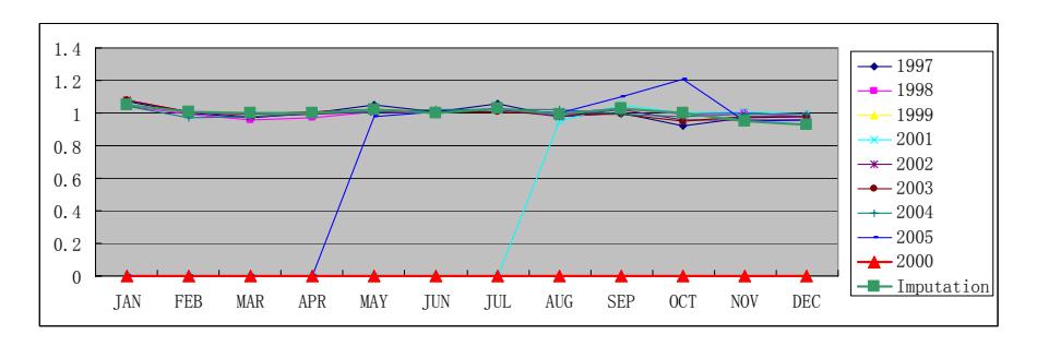
### **A.6 Imputation for Site 970267**
| | JAN | FEB | MAR | APR | MAY | JUN | JUL | AUG | SEP | OCT | NOV | DEC |
|------------|------|------|------|------|------|------|------|------|------|------|------|------|
| 1997 | 1.05 | 0.99 | 0.93 | 0.99 | 1.01 | 1.01 | 1.01 | 0.98 | 1 | 0.99 | 1.02 | 1.07 |
| 1998 | 1.05 | 1 | 0.97 | 1.03 | 1.03 | 1.01 | 1 | 0.99 | 1.04 | 1 | 0.97 | 0.94 |
| 1999 | 1.05 | 0.99 | 0.97 | 0.99 | 1.03 | 1.03 | 1.07 | 1.02 | 1.01 | 0.98 | 0.9 | 0.95 |
| 2000 | 0 | 0 | 0 | 0 | 0 | 0 | 0 | 0 | 0 | 0 | 0 | 0 |
| 2001 | | | | | | | | | | | | |
| 2002 | | | | | | | | | | | | |
| 2003 | | | | | | | | | | | | |
| 2004 | 0 | 0 | 0 | 0 | 0 | 0 | 0 | 0 | 0 | 0 | 0 | 0 |
| 2005 | 1.04 | 0.99 | 0.96 | 0.97 | 1 | 1 | 1 | 1.01 | 1.03 | 1.12 | 0.94 | 0.98 |
| | | | | | | | | | | | | |
| 2000 | 0 | 0 | 0 | 0 | 0 | 0 | 0 | 0 | 0 | 0 | 0 | 0 |
| Imputation | 1.05 | 0.99 | 0.97 | 0.99 | 1.03 | 1.03 | 1.02 | 1.02 | 1.01 | 0.98 | 0.96 | 0.95 |
| | | | | | | | Avg | | | | Avg | |
| Source | 1999 | 1999 | 1999 | 1999 | 1999 | 1999 | all | 1999 | 1999 | 1999 | all | 1999 |
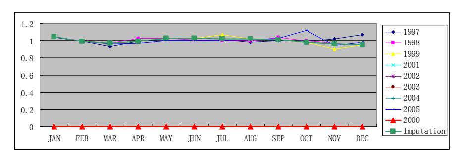
### **A.7 Imputation for Site 930257**
| | JAN | FEB | MAR | APR | MAY | JUN | JUL | AUG | SEP | OCT | NOV | DEC |
|------------|------|------|------|------|------|------|------|------|------|------|------|------|
| 1997 | 0.97 | 0.91 | 0.88 | 0.93 | 0.97 | 1.12 | 1.15 | 1.11 | 1.03 | 1.01 | 1.01 | 0.99 |
| 1998 | 1.05 | 0.99 | 0.91 | 0.93 | 0.96 | 1.09 | 1.14 | 1.09 | 1.08 | 1 | 0.89 | 1 |
| 1999 | 1 | 0.91 | 0.89 | 0.92 | 0.94 | 1.06 | 1.11 | 1.07 | 1.07 | 1.02 | 1.01 | 1.05 |
| 2000 | 1.05 | 1 | 0.95 | 0 | 0 | 0 | 0 | 0 | 0 | 0 | 0 | 0 |
| 2001 | | | | | | | | | | | | |
| 2002 | | | | | | | | | | | | |
| 2003 | 0.99 | 0.93 | 0.92 | 0.97 | 1.01 | 1.07 | 1.11 | 1.04 | 1.01 | 1.01 | 0.99 | 1.02 |
| 2004 | 1.04 | 0.95 | 0.93 | 0.93 | 0.98 | 1.11 | 1.12 | 1.09 | 1.16 | 0.94 | 0.97 | 0.87 |
| 2005 | 0.98 | 0.92 | 0.92 | 0.91 | 0.94 | 1.09 | 1.1 | 1.06 | 1.05 | 1.16 | 0.96 | 0.99 |
| | | | | | | | | | | | | |
| 2000 | 1.05 | 1 | 0.95 | 0 | 0 | 0 | 0 | 0 | 0 | 0 | 0 | 0 |
| Imputation | 1 | 0.91 | 0.89 | 0.92 | 0.94 | 1.06 | 1.11 | 1.07 | 1.07 | 1.02 | 1.01 | 1.05 |
| Source | 1999 | 1999 | 1999 | 1999 | 1999 | 1999 | 1999 | 1999 | 1999 | 1999 | 1999 | 1999 |
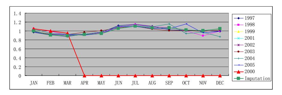
### **A.8 Imputation for Site 930174**
| | JAN | FEB | MAR | APR | MAY | JUN | JUL | AUG | SEP | OCT | NOV | DEC |
|------------|------|------|------|------|------|------|------|------|------|--------|------|------|
| | | | | | | | | | | | | |
| 1997 | 0.95 | 0.94 | 0.94 | 1 | 1.03 | 1.03 | 1.05 | 1.02 | 1.08 | 1.04 | 1 | 0.97 |
| 1998 | 0.98 | 0.94 | 0.93 | 0.95 | 1.01 | 1 | 1.04 | 1.1 | 1.13 | 1.02 | 1 | 0.98 |
| 1999 | 1.01 | 0.94 | 0.95 | 0.97 | 1.03 | 1.06 | 1.03 | 1.04 | 1.1 | 1.15 | 1.01 | 1.01 |
| 2000 | 0 | 0 | 0 | 0 | 0 | 0 | 0 | 0 | 0 | 0 | 0 | 0 |
| 2001 | | | | | | | | | | | | |
| 2002 | 0 | 0 | 0 | 0 | 0 | 0 | 0 | 0 | 0 | 0 | 1.02 | 0.98 |
| 2003 | 1.01 | 0.96 | 0.96 | 0.97 | 1.01 | 1.01 | 1.02 | 1 | 1.03 | 1 | 1 | 0.99 |
| 2004 | 1 | 0.95 | 0.93 | 0.95 | 0.99 | 1 | 1.02 | 1 | 1.34 | 0.98 | 0.99 | 0.97 |
| 2005 | 1.01 | 1.01 | 0.99 | 0 | 0 | 0 | 0 | 0 | 0 | 0 | 0 | 0 |
| | | | | | | | | | | | | |
| 2000 | 0 | 0 | 0 | 0 | 0 | 0 | 0 | 0 | 0 | 0 | 0 | 0 |
| Imputation | 1.01 | 0.94 | 0.95 | 0.97 | 1.03 | 1.06 | 1.03 | 1.04 | 1.1 | 1.01 | 1.01 | 1.01 |
| Source | 1999 | 1999 | 1999 | 1999 | 1999 | 1999 | 1999 | 1999 | 1999 | Avg-99 | 1999 | 1999 |
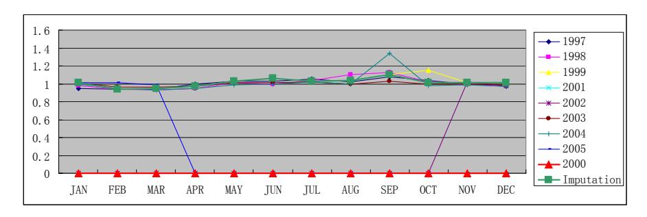
### **A.9 Imputation for Site 930099**
| | JAN | FEB | MAR | APR | MAY | JUN | JUL | AUG | SEP | OCT | NOV | DEC |
|------------|------|------|------|------|------|------|------|------|------|------|------|------|
| 1997 | 0.97 | 0.91 | 0.92 | 0.95 | 1.01 | 1.08 | 1.14 | 1.08 | 1.07 | 1 | 0.98 | 0.95 |
| 1998 | 0.95 | 0.91 | 0.91 | 0.94 | 0.99 | 1.04 | 1.11 | 1.07 | 1.11 | 1.04 | 1.04 | 1 |
| 1999 | 0.97 | 0.93 | 0.94 | 0.98 | 1 | 1.07 | 1.1 | 1.07 | 1.09 | 1.01 | 0.99 | 0.96 |
| 2000 | 0 | 0.89 | 0.9 | 0.94 | 0.99 | 0 | 0 | 1.12 | 1.13 | 0 | 0 | 0 |
| 2001 | | | | | | | | | | | | |
| 2002 | | | | | | | | | | | | |
| 2003 | 0 | 0 | 0 | 0 | 0 | 0 | 0 | 0 | 1.06 | 1.02 | 0.97 | 0.94 |
| 2004 | 1.03 | 0.95 | 0.94 | 0.94 | 1.01 | 1.04 | 1.07 | 1.04 | 1.22 | 0.98 | 0.93 | 0.94 |
| 2005 | 0.96 | 0.92 | 0.9 | 0.93 | 0.98 | 1.02 | 1.07 | 1.04 | 1.06 | 1.17 | 1.03 | 0.97 |
| | | | | | | | | | | | | |
| 2000 | 0 | 0.89 | 0.9 | 0.94 | 0.99 | 0 | 0 | 1.12 | 1.13 | 0 | 0 | 0 |
| Imputation | 0.97 | 0.93 | 0.94 | 0.98 | 1 | 1.07 | 1.1 | 1.07 | 1.09 | 1.01 | 0.99 | 0.96 |
| Source | 1999 | 1999 | 1999 | 1999 | 1999 | 1999 | 1999 | 1999 | 1999 | 1999 | 1999 | 1999 |
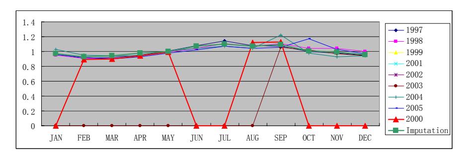
### **A.10 Imputation for Site 870187**
| | JAN | FEB | MAR | APR | MAY | JUN | JUL | AUG | SEP | OCT | NOV | DEC |
|------------|------|------|------|------|------|------|------|------|------|------|------|------|
| 1997 | 1.03 | 1 | 0.99 | 0.98 | 1 | 0.99 | 1.01 | 1 | 1.02 | 0.99 | 1 | 0.99 |
| 1998 | 1.03 | 1.01 | 0.99 | 0.99 | 1.01 | 1 | 1.02 | 1 | 1 | 0.97 | 1 | 1 |
| 1999 | 1.02 | 0.99 | 0.98 | 0.99 | 1 | 1.01 | 1.02 | 1 | 1.03 | 1 | 0.99 | 0.98 |
| 2000 | 1.02 | 1 | 0.98 | 1 | 0 | 0 | 0 | 0 | 0 | 0 | 0 | 0 |
| 2001 | | | | | | | | | | | | |
| 2002 | 0 | 0 | 0 | 0 | 0 | 0 | 0 | 0 | 0 | 0 | 0.98 | 1.01 |
| 2003 | 1.05 | 1 | 0.99 | 1.01 | 1.02 | 1 | 1.01 | 1 | 0.99 | 0.98 | 0.99 | 0.98 |
| 2004 | 0 | 0 | 0 | 0 | 0 | 0 | 0 | 0 | 0 | 0 | 0 | 0 |
| 2005 | | | | | | | | | | | | |
| | | | | | | | | | | | | |
| 2000 | 1.02 | 1 | 0.98 | 1 | 0 | 0 | 0 | 0 | 0 | 0 | 0 | 0 |
| Imputation | 1.02 | 0.99 | 0.98 | 0.99 | 1 | 1.01 | 1.02 | 1 | 1.03 | 1 | 0.99 | 0.98 |
| Source | 1999 | 1999 | 1999 | 1999 | 1999 | 1999 | 1999 | 1999 | 1999 | 1999 | 1999 | 1999 |
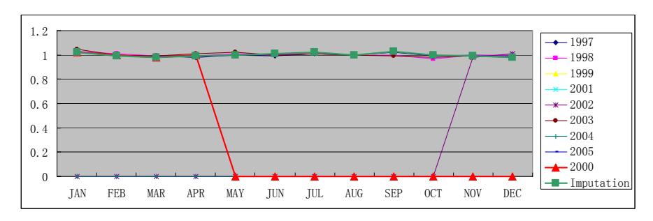
### **A.11 Imputation for Site 799929**
| | JAN | FEB | MAR | APR | MAY | JUN | JUL | AUG | SEP | OCT | NOV | DEC |
|------------|------|------|------|------|------|------|------|------|------|------|------|------|
| 1997 | 1.01 | 0.88 | 0.86 | 0.95 | 1.02 | 1.07 | 1.07 | 1.09 | 1.1 | 1.04 | 1 | 1 |
| 1998 | 0.93 | 0.9 | 0.88 | 0.91 | 1.03 | 1.07 | 1.1 | 1.11 | 1.1 | 1.02 | 1.01 | 1.01 |
| 1999 | 0.96 | 0.85 | 0.9 | 0.97 | 0.99 | 1.04 | 1.11 | 1.1 | 1.18 | 1.06 | 0.98 | 0.97 |
| 2000 | 0 | 0.94 | 0.9 | 0.95 | 1.04 | 1.07 | 1.11 | 0 | 0 | 0 | 0 | 0 |
| 2001 | 0.99 | 0.95 | 0.94 | 0.99 | 1.1 | 1.12 | 0 | 0 | 0 | 0 | 0 | 0 |
| 2002 | 0 | 0 | 0 | 0 | 0 | 0 | 0 | 1.04 | 1.04 | 0.98 | 0.97 | 0.99 |
| 2003 | 0.98 | 0.93 | 0.87 | 0.93 | 0.99 | 1.06 | 1.09 | 1.1 | 1.12 | 1.03 | 1.02 | 1.02 |
| 2004 | 0.99 | 0.9 | 0.87 | 0.95 | 1.01 | 1.07 | 1.07 | 1.05 | 1.17 | 0.99 | 0.99 | 1.03 |
| 2005 | 0.96 | 0.9 | 0.84 | 0.93 | 0.99 | 1.06 | 1.03 | 1.1 | 1.14 | 1.07 | 1.03 | 1.06 |
| | | | | | | | | | | | | |
| 2000 | 0 | 0.94 | 0.9 | 0.95 | 1.04 | 1.07 | 1.11 | 0 | 0 | 0 | 0 | 0 |
| Imputation | 0.96 | 0.9 | 0.9 | 0.97 | 0.99 | 1.04 | 1.11 | 1.1 | 1.13 | 1.06 | 0.98 | 0.97 |
| | | Avg | | | | | | | Avg | | | |
| Source | 1999 | all | 1999 | 1999 | 1999 | 1999 | 1999 | 1999 | 2002 | 1999 | 1999 | 1999 |
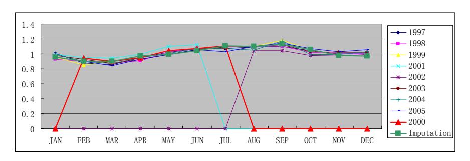
### **A.12 Imputation for Site 729923**
| | JAN | FEB | MAR | APR | MAY | JUN | JUL | AUG | SEP | OCT | NOV | DEC |
|------------|------|------|------|------|------|------|------|------|------|------|------|------|
| 1997 | 1.02 | 0.96 | 0.93 | 1 | 1.02 | 0.99 | 0.96 | 1.01 | 1.13 | 1.02 | 1.04 | 0.96 |
| 1998 | 1.06 | 1.01 | 1 | 0 | 1.13 | 0 | 0 | 0 | 1.09 | 0 | 0 | 0.83 |
| 1999 | 1.18 | 0.97 | 0.94 | 0.94 | 1 | 0.97 | 0.94 | 0.98 | 1.1 | 1.02 | 1.02 | 1.01 |
| 2000 | 1.09 | 1.02 | 0.97 | 0.99 | 1 | 0.99 | 0.98 | 0.99 | 0 | 0 | 0 | 0 |
| 2001 | | | | | | | | | | | | |
| 2002 | | | | | | | | | | | | |
| 2003 | | | | | | | | | | | | |
| 2004 | 0 | 0 | 0 | 0 | 0 | 0 | 0 | 0 | 0 | 0 | 0 | 0 |
| 2005 | 1.01 | 0.94 | 0.91 | 0.96 | 0.98 | 0.98 | 0.96 | 1.04 | 1.14 | 1.08 | 1.03 | 1.02 |
| | | | | | | | | | | | | |
| 2000 | 1.09 | 1.02 | 0.97 | 0.99 | 1 | 0.99 | 0.98 | 0.99 | 0 | 0 | 0 | 0 |
| Imputation | 1.09 | 1.02 | 0.97 | 0.99 | 1 | 0.99 | 0.98 | 0.99 | 1.1 | 1.02 | 1.02 | 1.01 |
| Source | 1999 | 1999 | 1999 | 1999 | 1999 | 1999 | 1999 | 1999 | 1999 | 1999 | 1999 | 1999 |
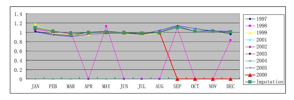
### **A.13 Imputation for Site 729914**
| | JAN | FEB | MAR | APR | MAY | JUN | JUL | AUG | SEP | OCT | NOV | DEC |
|------------|------|------|------|------|------|------|------|------|------|------|------|------|
| 1997 | | | | | | | | | | | | |
| 1998 | | | | | | | | | | | | |
| 1999 | 0 | 0 | 0 | 0 | 0 | 0 | 0 | 0 | 0 | 0 | 0 | 0 |
| 2000 | 0 | 0 | 0 | 1 | 0.98 | 1.02 | 1.03 | 1.04 | 1.01 | 1 | 0.98 | 1.05 |
| 2001 | 1 | 0.96 | 0.95 | 0.97 | 0.95 | 0.97 | 0.98 | 0.98 | 1.08 | 1.02 | 1.01 | 1.05 |
| 2002 | 1.12 | 0.99 | 0.94 | 1 | 1 | 0.98 | 0.99 | 1 | 1.04 | 0.99 | 0.98 | 1.01 |
| 2003 | | | | | | | | | | | | |
| 2004 | 0 | 0 | 0 | 0 | 0 | 0 | 0 | 0 | 0 | 0 | 0 | 0 |
| 2005 | 1.05 | 1 | 0.98 | 0.98 | 1 | 1.02 | 0 | 0 | 0 | 0 | 0 | 0 |
| | | | | | | | | | | | | |
| 2000 | 0 | 0 | 0 | 1 | 0.98 | 1.02 | 1.03 | 1.04 | 1.01 | 1 | 0.98 | 1.05 |
| Imputation | 1 | 0.96 | 0.95 | 1 | 0.98 | 1.02 | 1.03 | 1.04 | 1.01 | 1 | 0.98 | 1.05 |
| Source | 2001 | 2001 | 2001 | 2000 | 2000 | 2000 | 2000 | 2000 | 2000 | 2000 | 2000 | 2000 |
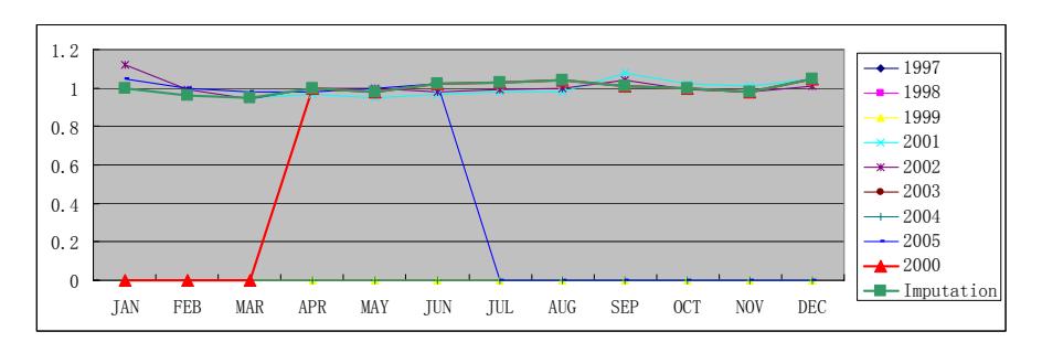
### **A.14 Imputation for Site 710189**
| | JAN | FEB | MAR | APR | MAY | JUN | JUL | AUG | SEP | OCT | NOV | DEC |
|------------|------|------|------|------|------|------|------|------|------|------|------|------|
| 1997 | 1.06 | 1 | 0.98 | 0.98 | 0.98 | 0.99 | 1.01 | 0.99 | 0.99 | 0.99 | 1 | 1.02 |
| 1998 | 1.05 | 1.01 | 0.98 | 0.96 | 0.97 | 1 | 0.98 | 1.01 | 1.02 | 0.99 | 1.02 | 1.02 |
| 1999 | 1.07 | 1 | 0.98 | 0.97 | 0.98 | 1 | 1.02 | 1.01 | 0 | 0 | 0 | 0 |
| 2000 | 0 | 0 | 0 | 0 | 0 | 0 | 0 | 0 | 0 | 0.97 | 1.02 | 1.01 |
| 2001 | 1.08 | 1.01 | 1.02 | 0.94 | 0.96 | 0.99 | 1.02 | 1.05 | 1.06 | 0.98 | 0.99 | 0.98 |
| 2002 | 1.08 | 1.01 | 0.99 | 0.95 | 0.99 | 1.04 | 0.99 | 0.99 | 1 | 0.98 | 1.01 | 0.99 |
| 2003 | 1.07 | 1.01 | 0.99 | 0.95 | 0.97 | 1.02 | 1.03 | 0.99 | 0.98 | 0.99 | 1 | 1 |
| 2004 | 1.05 | 1.01 | 0.97 | 0.95 | 0.97 | 1.01 | 1.02 | 1 | 1.06 | 0.97 | 1 | 1 |
| 2005 | 1.06 | 1.01 | 1 | 0.96 | 0.99 | 1 | 1.03 | 0.98 | 1 | 0.98 | 1 | 0.99 |
| | | | | | | | | | | | | |
| 2000 | 0 | 0 | 0 | 0 | 0 | 0 | 0 | 0 | 0 | 0.97 | 1.02 | 1.01 |
| Imputation | 1.06 | 1 | 0.98 | 0.98 | 0.98 | 0.99 | 1.01 | 0.99 | 0.99 | 0.99 | 1 | 1.02 |
| Source | 1997 | 1997 | 1997 | 1997 | 1997 | 1997 | 1997 | 1997 | 1997 | 1997 | 1997 | 1997 |
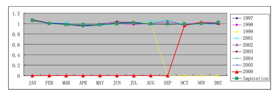
### **A.15 Imputation for Site 589937**
| | JAN | FEB | MAR | APR | MAY | JUN | JUL | AUG | SEP | OCT | NOV | DEC |
|------------|------|------|------|------|------|------|------|------|------|------|------|------|
| 1997 | 1.05 | 1.04 | 0.98 | 1.01 | 0.98 | 0.95 | 1 | 0.97 | 1 | 0.98 | 1.02 | 1.04 |
| 1998 | 1.1 | 1.09 | 0.96 | 0.98 | 0.97 | 0.96 | 0.99 | 0.99 | 1.05 | 1.02 | 1.06 | 1 |
| 1999 | 1.04 | 1 | 0.99 | 0.97 | 0.98 | 0.96 | 0.98 | 0.97 | 1.04 | 1.02 | 1.05 | 1.09 |
| 2000 | 1.04 | 1 | 0.99 | 0.97 | 0.98 | 0.98 | 1.02 | 1 | 1.02 | 0 | 0 | 0 |
| 2001 | | | | | | | | | | | | |
| 2002 | 0 | 0 | 0 | 0 | 1.03 | 0.98 | 0.99 | 0.97 | 1.03 | 1.01 | 1.04 | 0.97 |
| 2003 | 1.1 | 1.05 | 1.01 | 1 | 1.03 | 0.98 | 0.98 | 0.96 | 0.98 | 0.97 | 0.99 | 1.02 |
| 2004 | 1.1 | 1.03 | 1 | 0.98 | 0.99 | 0.99 | 0.99 | 0.97 | 1.02 | 0.94 | 0.99 | 1.01 |
| 2005 | 0.98 | 0.96 | 0.96 | 0.97 | 0.98 | 0.98 | 1 | 1 | 1.04 | 1.02 | 1.06 | 1.08 |
| | | | | | | | | | | | | |
| 2000 | 1.04 | 1 | 0.99 | 0.97 | 0.98 | 0.98 | 1.02 | 1 | 1.02 | 0 | 0 | 0 |
| Imputation | 1.04 | 1 | 0.99 | 0.97 | 0.98 | 0.96 | 0.98 | 0.97 | 1.04 | 1.02 | 1.05 | 1.01 |
| Source | 1999 | 1999 | 1999 | 1999 | 1999 | 1999 | 1999 | 1999 | 1999 | 1999 | 1999 | 1999 |
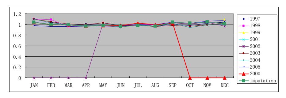
### **A.16 Imputation for Site 559908**
| | JAN | FEB | MAR | APR | MAY | JUN | JUL | AUG | SEP | OCT | NOV | DEC |
|------------|------|------|------|------|------|------|------|------|------|------|------|------|
| 1997 | 1.08 | 1.01 | 0.98 | 0.98 | 0.97 | 0.94 | 0.97 | 0.98 | 1 | 1 | 1.04 | 1.05 |
| 1998 | 1.09 | 1.03 | 1 | 0.98 | 0.96 | 0.95 | 0.97 | 0.98 | 1.04 | 0.98 | 1 | 1.02 |
| 1999 | 1.09 | 1.01 | 0.99 | 0.99 | 0.99 | 0.98 | 0.99 | 0.99 | 0 | 0 | 0 | 0 |
| 2000 | 0 | 0 | 0 | 0 | 0 | 1 | 1 | 0.98 | 1.02 | 0.98 | 1.01 | 1 |
| 2001 | 1.07 | 1.01 | 1 | 0.96 | 0.97 | 0.96 | 0.98 | 1 | 1.01 | 1 | 1.02 | 1.02 |
| 2002 | 1.07 | 1 | 0.98 | 0.95 | 0.97 | 0.97 | 0.97 | 0.99 | 1.02 | 1.01 | 1.05 | 1.05 |
| 2003 | 1.09 | 1.02 | 1 | 0.96 | 0.95 | 0.97 | 0.99 | 0.98 | 1 | 0.99 | 1.04 | 1.03 |
| 2004 | 0 | 0 | 0 | 0 | 0 | 0 | 0 | 0 | 0 | 0 | 0 | 0 |
| 2005 | | | | | | | | | | | | |
| | | | | | | | | | | | | |
| 2000 | 0 | 0 | 0 | 0 | 0 | 1 | 1 | 0.98 | 1.02 | 0.98 | 1.01 | 1 |
| Imputation | 1.07 | 1.01 | 1 | 0.96 | 0.97 | 0.96 | 0.98 | 1 | 1.01 | 1 | 1.02 | 1.02 |
| Source | 2001 | 2001 | 2001 | 2001 | 2001 | 2001 | 2001 | 2001 | 2001 | 2001 | 2001 | 2001 |
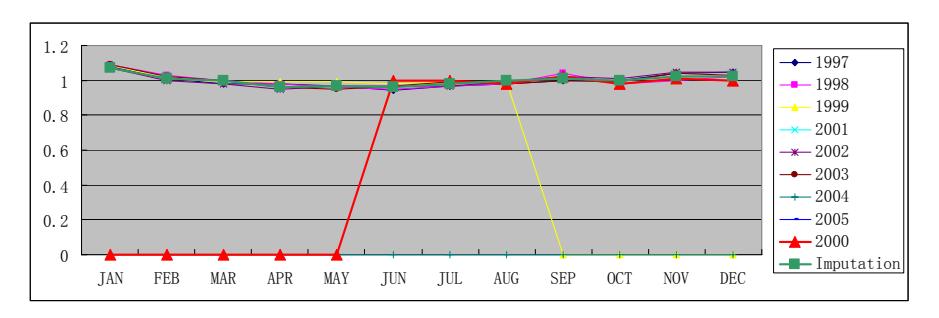
### **A.17 Imputation for Site 550207**
| | JAN | FEB | MAR | APR | MAY | JUN | JUL | AUG | SEP | OCT | NOV | DEC |
|------------|------|------|------|------|------|------|------|------|------|------|------|------|
| 1997 | 1.04 | 0.98 | 0.98 | 0.99 | 1 | 1.02 | 1.03 | 1 | 0.99 | 0.98 | 1.02 | 0.99 |
| 1998 | 1.02 | 0.98 | 0.97 | 0.98 | 0.98 | 1 | 1.04 | 0.99 | 1.04 | 0.99 | 1.02 | 1 |
| 1999 | 1.03 | 0.97 | 0.97 | 1.02 | 1.13 | 0 | 0 | 0 | 0 | 0 | 0 | 0 |
| 2000 | 0 | 0 | 0.95 | 0.91 | 0.91 | 1.01 | 1.25 | 0 | 1.07 | 1 | 0.94 | 1.01 |
| 2001 | 1.04 | 0.97 | 1.04 | 0.94 | 0.98 | 1.01 | 1.04 | 1 | 1 | 0.98 | 1.04 | 0.98 |
| 2002 | 1.04 | 0.98 | 1.06 | 0.95 | 0.99 | 1 | 1.03 | 1 | 0.98 | 0.99 | 1.07 | 0.97 |
| 2003 | 1.05 | 0.99 | 1.02 | 1 | 1 | 1.01 | 1.06 | 1.01 | 0.98 | 0.98 | 1 | 0.98 |
| 2004 | 1.05 | 1 | 0.99 | 0.97 | 0.98 | 1.01 | 1.04 | 0.99 | 1.01 | 0.95 | 1.01 | 1 |
| 2005 | 1 | 0.96 | 1 | 0.96 | 0.98 | 1.02 | 1.06 | 1.01 | 1.02 | 0.97 | 1.04 | 1 |
| | | | | | | | | | | | | |
| 2000 | 0 | 0 | 0.95 | 0.91 | 0.91 | 1.01 | 1.25 | 0 | 1.07 | 1 | 0.94 | 1.01 |
| Imputation | 1.04 | 0.97 | 1.04 | 0.94 | 0.98 | 1.01 | 1.04 | 1 | 1 | 0.98 | 1.04 | 0.98 |
| Source | 2001 | 2001 | 2001 | 2001 | 2001 | 2001 | 2001 | 2001 | 2001 | 2001 | 2001 | 2001 |
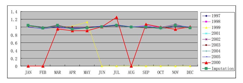
### **A.18 Imputation for Site 530117**
| | JAN | FEB | MAR | APR | MAY | JUN | JUL | AUG | SEP | OCT | NOV | DEC |
|------------|------|------|------|------|------|------|------|------|------|------|------|------|
| 1997 | 1.07 | 0.99 | 0.97 | 0.99 | 0.99 | 0.99 | 1 | 0.97 | 1 | 0.98 | 1.05 | 1.02 |
| 1998 | 1.05 | 0.99 | 0.97 | 0.99 | 0.99 | 0.99 | 1 | 0.97 | 1.02 | 1 | 1.02 | 1.02 |
| 1999 | 1.03 | 0.97 | 0.99 | 0.95 | 0.99 | 1 | 1.05 | 0.97 | 1.01 | 1.01 | 1.03 | 1.03 |
| 2000 | 1.07 | 1 | 1 | 0.99 | 0 | 0 | 0 | 0 | 0 | 0.97 | 1 | 0.99 |
| 2001 | 1.08 | 0.98 | 1 | 0.94 | 0.93 | 0.98 | 1.03 | 1 | 1.02 | 1.01 | 1.04 | 1.03 |
| 2002 | 1.02 | 0.95 | 0.99 | 0.97 | 0.99 | 0.99 | 1.02 | 0.99 | 1.03 | 1.01 | 1.03 | 1.02 |
| 2003 | 1.04 | 0.98 | 0.98 | 0.97 | 0.98 | 0.99 | 1 | 0.97 | 1.01 | 1.01 | 1.04 | 1.04 |
| 2004 | 1.05 | 0.99 | 0.98 | 0.97 | 1 | 0.99 | 1 | 0.99 | 1.04 | 0.97 | 1.02 | 1.02 |
| 2005 | 1.01 | 0.96 | 1 | 0.98 | 0.99 | 0.99 | 1.02 | 1 | 1.04 | 0.98 | 1.02 | 1 |
| | | | | | | | | | | | | |
| 2000 | 1.07 | 1 | 1 | 0.99 | 0 | 0 | 0 | 0 | 0 | 0.97 | 1 | 0.99 |
| Imputation | 1.08 | 0.98 | 1 | 0.94 | 0.93 | 0.98 | 1.03 | 1 | 1.02 | 1.01 | 1.04 | 1.03 |
| Source | 2001 | 2001 | 2001 | 2001 | 2001 | 2001 | 2001 | 2001 | 2001 | 2001 | 2001 | 2001 |
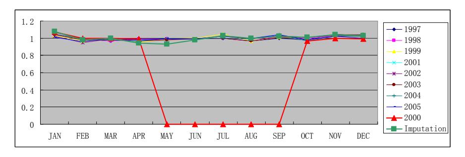
### **A.19 Imputation for Site 509904**
| | JAN | FEB | MAR | APR | MAY | JUN | JUL | AUG | SEP | OCT | NOV | DEC |
|------------|------|------|------|------|------|------|------|------|------|------|------|------|
| 1997 | | | | | | | | | | | | |
| 1998 | 0 | 0 | 0 | 1.01 | 1.02 | 0.98 | 1.03 | 1 | 1.01 | 0.95 | 1 | 1 |
| 1999 | 1.1 | 1.01 | 0.99 | 0.98 | 0.99 | 0.98 | 1.01 | 1 | 0.97 | 0.94 | 0.99 | 1 |
| 2000 | 1.02 | 0.95 | 0 | 0 | 0 | 0 | 0 | 0 | 0 | 0.98 | 1.01 | 1.04 |
| 2001 | 1.02 | 0.98 | 0.97 | 0.94 | 0.98 | 0.96 | 1 | 1.04 | 1.03 | 1.01 | 1.02 | 1.05 |
| 2002 | 1.11 | 1.02 | 1.04 | 1.02 | 1.02 | 1.01 | 1.01 | 1 | 1.03 | 0.92 | 0.93 | 0.92 |
| 2003 | 1.11 | 1.03 | 1.06 | 0.99 | 0.97 | 0.97 | 1 | 1 | 1 | 0.98 | 1 | 0.98 |
| 2004 | 1.07 | 1.02 | 0.98 | 0.98 | 0.97 | 0.96 | 0.99 | 1 | 1.05 | 0.99 | 1 | 1.01 |
| 2005 | 1.04 | 0.96 | 0.97 | 0.97 | 0.97 | 0.98 | 1 | 1.02 | 1.05 | 1.01 | 1.05 | 1.05 |
| | | | | | | | | | | | | |
| 2000 | 1.02 | 0.95 | 0 | 0 | 0 | 0 | 0 | 0 | 0 | 0.98 | 1.01 | 1.04 |
| Imputation | 1.02 | 0.98 | 0.97 | 0.94 | 0.98 | 0.96 | 1 | 1.04 | 1.03 | 1.01 | 1.02 | 1.05 |
| Source | 2001 | 2001 | 2001 | 2001 | 2001 | 2001 | 2001 | 2001 | 2001 | 2001 | 2001 | 2001 |
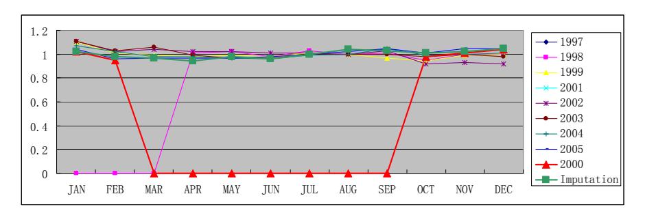
### **A.20 Imputation for Site 480159**
| | JAN | FEB | MAR | APR | MAY | JUN | JUL | AUG | SEP | OCT | NOV | DEC |
|------------|------|------|------|------|------|------|------|------|------|------|------|------|
| 1997 | 1.07 | 1.02 | 0.97 | 0.99 | 0.99 | 0.98 | 0 | 0 | 0 | 0 | 0 | 0 |
| 1998 | 1.09 | 1.02 | 0.99 | 1.01 | 0.96 | 0.97 | 0.98 | 0.98 | 1.05 | 0.99 | 1 | 0.99 |
| 1999 | 1.07 | 1.01 | 0.99 | 0.97 | 0.98 | 0.98 | 0.98 | 1 | 1.01 | 0.98 | 1 | 1.04 |
| 2000 | 0 | 0 | 0 | 0 | 0 | 0 | 0 | 0 | 0 | 0 | 0 | 0 |
| 2001 | | | | | | | | | | | | |
| 2002 | | | | | | | | | | | | |
| 2003 | | | | | | | | | | | | |
| 2004 | | | | | | | | | | | | |
| 2005 | | | | | | | | | | | | |
| | | | | | | | | | | | | |
| 2000 | 0 | 0 | 0 | 0 | 0 | 0 | 0 | 0 | 0 | 0 | 0 | 0 |
| Imputation | 1.07 | 1.01 | 0.99 | 0.97 | 0.98 | 0.98 | 0.98 | 1 | 1.01 | 0.98 | 1 | 1.04 |
| Source | 1999 | 1999 | 1999 | 1999 | 1999 | 1999 | 1999 | 1999 | 1999 | 1999 | 1999 | 1999 |
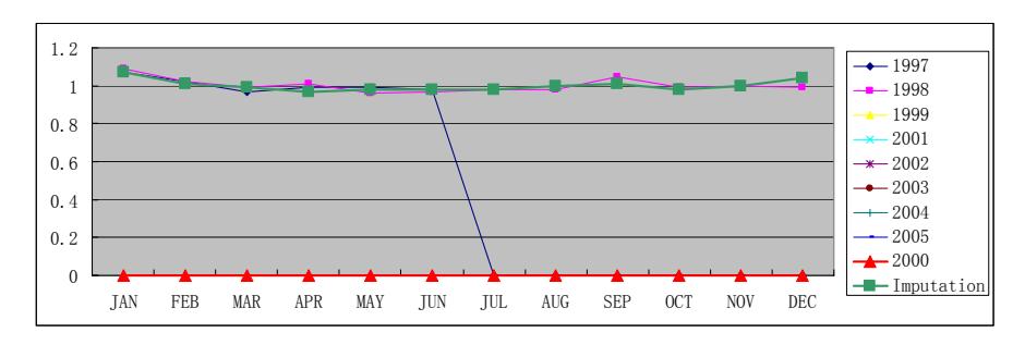
### **A.21 Imputation for Site 460305**
| | JAN | FEB | MAR | APR | MAY | JUN | JUL | AUG | SEP | OCT | NOV | DEC |
|------------|------|------|------|------|------|------|------|------|------|------|------|------|
| 1997 | 1.14 | 1.03 | 0.89 | 0.97 | 0.94 | 0.88 | 0.87 | 0.92 | 1.03 | 1.08 | 1.17 | 1.2 |
| 1998 | 1.16 | 1.04 | 0.92 | 0.95 | 0.96 | 0.88 | 0.88 | 0.96 | 1.17 | 1.17 | 1.18 | 1.19 |
| 1999 | 1.16 | 1.03 | 0.91 | 0.96 | 0.97 | 0.91 | 0.88 | 0.93 | 1.04 | 1.08 | 1.15 | 1.22 |
| 2000 | 1 | 0 | 0 | 0 | 0 | 0 | 0 | 0 | 0 | 0 | 0 | 0 |
| 2001 | 1.16 | 1 | 0.92 | 0.95 | 0.95 | 0.92 | 0.89 | 1 | 1.07 | 1.08 | 1.13 | 1.18 |
| 2002 | 1.17 | 1.02 | 0.92 | 0.96 | 0.97 | 0 | 0 | 0 | 0 | 0 | 0 | 0 |
| 2003 | | | | | | | | | | | | |
| 2004 | | | | | | | | | | | | |
| 2005 | | | | | | | | | | | | |
| | | | | | | | | | | | | |
| 2000 | 1 | 0 | 0 | 0 | 0 | 0 | 0 | 0 | 0 | 0 | 0 | 0 |
| Imputation | 1.16 | 1.03 | 0.91 | 0.96 | 0.97 | 0.91 | 0.88 | 0.93 | 1.04 | 1.08 | 1.15 | 1.22 |
| Source | 1999 | 1999 | 1999 | 1999 | 1999 | 1999 | 1999 | 1999 | 1999 | 1999 | 1999 | 1999 |
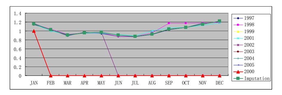
### **A.22 Imputation for Site 360317**
| | JAN | FEB | MAR | APR | MAY | JUN | JUL | AUG | SEP | OCT | NOV | DEC |
|------------|------|------|------|------|------|------|------|------|--------|------|-----------|------|
| 1997 | 1.11 | 1.04 | 0.91 | 0.99 | 1.06 | 0.99 | 0.94 | 0.97 | 1.16 | 1.05 | 0.95 | 0.94 |
| 1998 | 1.09 | 1.04 | 0.96 | 0.98 | 1.04 | 0.99 | 0.91 | 1.01 | 1.12 | 1.05 | 0.94 | 0.94 |
| 1999 | 1.11 | 1.03 | 0.93 | 0.92 | 1.03 | 0.99 | 0.95 | 1.04 | 1.04 | 1.06 | 0.92 | 1.05 |
| 2000 | 1.1 | 1.03 | 0.95 | 0.93 | | | | | | 1.05 | 0.97 | 1 |
| 2001 | 1.11 | 1.03 | 0.92 | 0.92 | 1.11 | 0.99 | 0.98 | 1.05 | 1.13 | 1.05 | 0.9 | 0.91 |
| 2002 | 1.08 | 0.99 | 0.88 | 0.98 | 1.03 | 0.99 | 0.9 | 1.08 | 1.17 | 1.06 | 1 | 0.94 |
| 2003 | 1.09 | 1 | 0.91 | 0.96 | 1.04 | 1.02 | 0.93 | 1.03 | 1.15 | 1.04 | 0.95 | 0.94 |
| 2004 | 1.1 | 1.04 | 0.91 | 0.95 | 1.05 | 1.01 | 0.96 | 1.08 | 1.16 | 1.02 | 1.05 | 0.8 |
| 2005 | 1.05 | 1.02 | 0.88 | 0.99 | 1.01 | 0.98 | 0.94 | 1.1 | 1.16 | 1.05 | 0.92 | 0.96 |
| | | | | | | | | | | | | |
| 2000 | 1.1 | 1.03 | 0.95 | 0.93 | | | | | | 1.05 | 0.97 | 1 |
| Imputation | 1.11 | 1.03 | 0.93 | 0.92 | 1.03 | 0.99 | 0.95 | 1.04 | 1.15 | 1.05 | 0.97 | 1 |
| Source | 1999 | 1999 | 1999 | 1999 | 1999 | 1999 | 1999 | 1999 | Avg-99 | 2000 | 2000 2000 | |
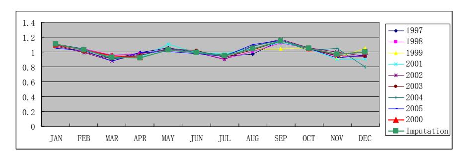
### **A.23 Imputation for Site 150086**
| | JAN | FEB | MAR | APR | MAY | JUN | JUL | AUG | SEP | OCT | NOV | DEC |
|------------|------|------|------|------|------|------|------|------|------|------|------|------|
| 1997 | | | | | | | | | | | | |
| 1998 | 0 | 0 | 0 | 0.92 | 1 | 0.98 | 1.02 | 1.02 | 0 | 1.01 | 1.04 | 1.04 |
| 1999 | 1.06 | 0.97 | 0.94 | 0.94 | 0.95 | 0.98 | 1.03 | 1.03 | 1.04 | 1.03 | 1.04 | 1.03 |
| 2000 | 1.06 | 0.95 | 0.93 | 0.94 | 0.97 | 1 | 1.05 | | | 1.05 | | |
| 2001 | 0.99 | 0.95 | 0.99 | 0.93 | 0.95 | 0.97 | 1 | 1 | 1.1 | 1.06 | 1.11 | 1.11 |
| 2002 | 1.08 | 1 | 0.96 | 0.93 | 0.96 | 1 | 1.02 | 1 | 1.06 | 1 | 1.01 | 1.02 |
| 2003 | 1.07 | 0.96 | 0.95 | 0.94 | 0.97 | 0.99 | 1 | 1 | 1.02 | 1.01 | 1.03 | 1.07 |
| 2004 | 1.05 | 0.95 | 0.9 | 0.94 | 0.97 | 1 | 1.02 | 1.04 | 1.07 | 1 | 1.02 | 1.05 |
| 2005 | 1.02 | 0.96 | 0.94 | 0.93 | 0.96 | 0.98 | 1 | 1.02 | 1.08 | 1.04 | 1.03 | 1.07 |
| | | | | | | | | | | | | |
| 2000 | 1.06 | 0.95 | 0.93 | 0.94 | 0.97 | 1 | 1.05 | | | 1.05 | | |
| Imputation | 1.06 | 0.95 | 0.93 | 0.94 | 0.97 | 1 | 1.05 | 1.03 | 1.04 | 1.03 | 1.04 | 1.03 |
| Source | 2000 | 2000 | 2000 | 2000 | 2000 | 2000 | 2000 | 1999 | 1999 | 1999 | 1999 | 1999 |
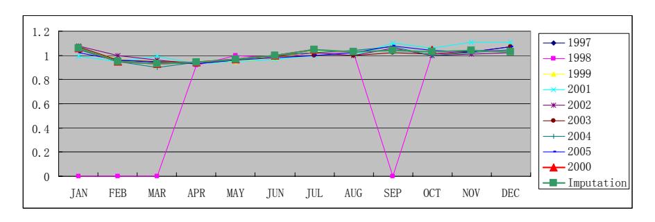
### **A.24 Imputation for Site 140199**
| | JAN | FEB | MAR | APR | MAY | JUN | JUL | AUG | SEP | OCT | NOV | DEC |
|------------|------|------|------|------|------|------|------|------|------|------|------|------|
| 1997 | 1 | 0.94 | 0.94 | 0.98 | 1.03 | 1.05 | 1.07 | 1.03 | 1.02 | 0.99 | 0.97 | 1 |
| 1998 | 1 | 0.95 | 0.94 | 0.99 | 1.03 | 1.05 | 1.05 | 1.03 | 1.06 | 0.98 | 0.95 | 0.97 |
| 1999 | | | | | | | | | | | | |
| 2000 | | | | | | | | | 1.05 | 1 | 0.99 | 0.97 |
| 2001 | 0.99 | 0.93 | 0.94 | 0.97 | 1.01 | 1.02 | 1.03 | 1.02 | 1.08 | 1.02 | 1 | 0.99 |
| 2002 | 1 | 0.94 | 0.93 | 0.97 | 1 | 1.03 | 1.05 | 1.03 | 1.04 | 1.01 | 1.01 | 1 |
| 2003 | 1.02 | 0.96 | 0.94 | 0.97 | 1 | 1.03 | 1.03 | 1.03 | 1.04 | 1 | 1 | 1 |
| 2004 | 1 | 0.94 | 0.91 | 0.97 | 1.01 | 1.02 | 1.04 | 1.06 | 1.11 | 0.99 | 1 | 0.99 |
| 2005 | 0.98 | 0.93 | 0.94 | 0.96 | 1 | 1.02 | 1.04 | 1.03 | 1.07 | 1.03 | 1.02 | 1 |
| | | | | | | | | | | | | |
| 2000 | 0 | 0 | 0 | 0 | 0 | 0 | 0 | 0 | 1.05 | 1 | 0.99 | 0.97 |
| Imputation | 0.99 | 0.93 | 0.94 | 0.97 | 1.01 | 1.02 | 1.03 | 1.02 | 1.08 | 1.02 | 1 | 0.99 |
| Source | 2001 | 2001 | 2001 | 2001 | 2001 | 2001 | 2001 | 2001 | 2001 | 2001 | 2001 | 2001 |
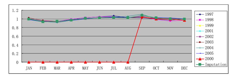
### **A.25 Imputation for Site 140013**
| | JAN | FEB | MAR | APR | MAY | JUN | JUL | AUG | SEP | OCT | NOV | DEC |
|------------|------|------|------|------|------|------|------|------|------|------|------|------|
| 1997 | 1.02 | 1.04 | 0.98 | 1 | 0.99 | 1 | 1.01 | 1 | 1 | 1 | 1.01 | 1.01 |
| 1998 | 1 | 0.99 | 0.98 | 0.99 | 1.01 | 1 | 1.02 | 0 | 0 | 0 | 0 | 0 |
| 1999 | | | | | | | | | | | | |
| 2000 | | | | | | 1.12 | 1.14 | 0.99 | 0.96 | 0.95 | 0.96 | 0.95 |
| 2001 | 0.93 | 0.97 | 0.97 | 0.95 | 0.98 | 1.03 | 1.07 | 1.02 | 1.09 | 1 | 1 | 0.99 |
| 2002 | 1.03 | 0.99 | 0.98 | 0.99 | 1.01 | 1.03 | 1.05 | 0.99 | 1 | 0.98 | 0.99 | 0.99 |
| 2003 | 1.08 | 1.01 | 1 | 1 | 1.01 | 1.01 | 1.02 | 0.99 | 0.98 | 0.95 | 0.97 | 0.98 |
| 2004 | 1.03 | 0.99 | 0.98 | 0.99 | 1 | 1.01 | 1.03 | 1.01 | 1.05 | 0.96 | 0.98 | 0.98 |
| 2005 | 1.02 | 0.98 | 0.98 | 0.98 | 1 | 1 | 1.04 | 1 | 1.02 | 1 | 1 | 1 |
| | | | | | | | | | | | | |
| 2000 | | | | | | 1.12 | 1.14 | 0.99 | 0.96 | 0.95 | 0.96 | 0.95 |
| Imputation | 1.03 | 0.99 | 0.98 | 0.99 | 1.01 | 1.03 | 1.05 | 0.99 | 1 | 0.98 | 0.99 | 0.99 |
| Source | 2002 | 2002 | 2002 | 2002 | 2002 | 2002 | 2002 | 2002 | 2002 | 2002 | 2002 | 2002 |
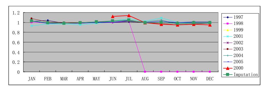
### **A.26 Imputation for Site 109922**
| | JAN | FEB | MAR | APR | MAY | JUN | JUL | AUG | SEP | OCT | NOV | DEC |
|------------|------|------|------|------|------|------|------|------|------|------|------|------|
| 1997 | 1.07 | 1 | 0.97 | 1.01 | 1.02 | 1.02 | 0.98 | 1 | 1 | 1 | 0.98 | 0.97 |
| 1998 | 1.02 | 1.01 | 0.98 | 0.98 | 1.02 | 0 | 0 | 1.02 | 0 | 0 | 1.01 | 0.98 |
| 1999 | 1.03 | 0.96 | 0.96 | 0.96 | 1 | 0.99 | 1 | 1 | 1.09 | 1.02 | 1 | 1 |
| 2000 | | | | 0.98 | 1.01 | 1.03 | | | | | | |
| 2001 | | | | | | | | | | | | |
| 2002 | | | | | | | | | | | | |
| 2003 | 0 | 0 | 0 | 0 | 0 | 0 | 1.01 | 1.02 | 1.02 | 0.99 | 0.98 | 0.99 |
| 2004 | 1.05 | 1 | 0.96 | 0.98 | 0.99 | 1 | 1 | 1.03 | 1.09 | 0.97 | 0.99 | 0.99 |
| 2005 | 1.01 | 0.98 | 0.96 | 0.98 | 0.99 | 1 | 1.02 | 1.01 | 1.04 | 1.02 | 1 | 1 |
| | | | | | | | | | | | | |
| 2000 | | | | 0.98 | 1.01 | 1.03 | | | | | | |
| Imputation | 1.03 | 0.96 | 0.96 | 0.96 | 1 | 0.99 | 1 | 1 | 1.09 | 1.02 | 1 | 1 |
| Source | 1999 | 1999 | 1999 | 1999 | 1999 | 1999 | 1999 | 1999 | 1999 | 1999 | 1999 | 1999 |
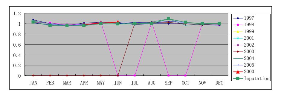
### **APPENDIX B. IMPUTATION OF MSFS FOR RURAL AREA**
### **B.1 Imputation for Site 010014**
For site 010014, data of year 2000 are borrowed from 2001.
| | JAN | FEB | MAR | APR | MAY | JUN | JUL | AUG | SEP | OCT | NOV | DEC |
|----------------|-------|-------|-------|-------|-------|-------|-------|-------|-------|-------|-------|-------|
| 1998 | 0.915 | 0.845 | 0.83 | 0.96 | 1.035 | 1.09 | 1.095 | 1.125 | 1.14 | 1.04 | 0.99 | 0.98 |
| 1999 | 0.94 | 0.865 | 0.85 | 0.995 | 1.075 | 1.135 | 1.1 | 1.1 | 1.095 | 1.05 | 0.995 | 1.005 |
| 2001 | 0.945 | 0.865 | 0.86 | 0.95 | 1.06 | 1.115 | 1.115 | 1.115 | 1.135 | 1.065 | 0.99 | 0.995 |
| 2002 | 0.945 | 0.865 | 0.85 | 0.965 | 1.055 | 1.095 | 1.105 | 1.1 | 1.11 | 1.04 | 0.975 | 0.99 |
| 2003 | 1.035 | 0.975 | 0.965 | | | | | | | | | |
| 2004 | | | | | | | | | | | | |
| 2005 | | | | | | | | | | | | |
| | | | | | | | | | | | | |
| 2000 | | | 0.835 | 0.925 | 1.02 | 1.055 | 1.045 | 1.055 | 1.055 | 1.005 | 0.95 | 0.94 |
| Imputatio
n | 0.95 | 0.87 | 0.86 | 0.95 | 1.06 | 1.12 | 1.12 | 1.12 | 1.14 | 1.07 | 0.99 | 1 |
| Source | 2001 | 2001 | 2001 | 2001 | 2001 | 2001 | 2001 | 2001 | 2001 | 2001 | 2001 | 2001 |
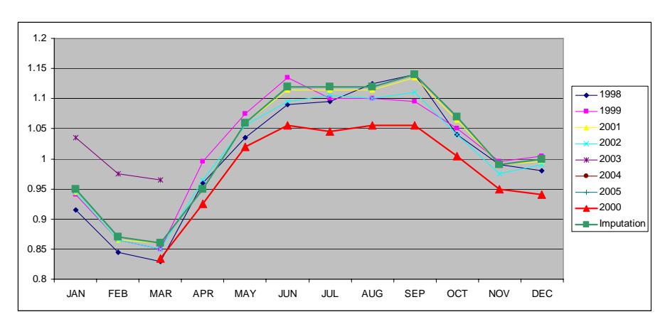
### **B.2 Imputation for Site 010350**
For site 010350, data for year 2000 are borrowed from 2001.
| | JAN | FEB | MAR APR | | MAY JUN | | JUL | AUG | SEP | OCT | NOV | DEC |
|------------|-------|-------|---------|-------|---------|-------|-------|-------|-------|------|-------|-------|
| 1998 | | | | | | | | | | | | |
| 1999 | | | | | | | | | | | | |
| 2001 | 0.94 | 0.865 | 0.82 | 0.925 | 1.04 | 1.045 | 1.05 | 1.08 | 1.145 | 1.07 | 0.995 | 1.045 |
| 2002 | 1.04 | 0.915 | 0.86 | 0.97 | 1.09 | 1.13 | 1.17 | | | | | |
| 2003 | | | 0.83 | 0.93 | | 1.045 | 1.035 | 1.07 | 1.15 | 1.03 | 0.96 | 0.99 |
| 2004 | 1.07 | 0.96 | 0.9 | 0.98 | 1.09 | 1.095 | 1.08 | 1.15 | 1.08 | 0.99 | 0.95 | 0.975 |
| 2005 | 1.065 | 0.985 | 0.935 | 1.07 | | | | | | | | |
| | | | | | | | | | | | | |
| 2000 | | | | 0.875 | 0.99 | 1.005 | 1.015 | 1.045 | 1.05 | 1.04 | 0.98 | 0.975 |
| Imputation | 0.94 | 0.87 | 0.82 | 0.93 | 1.04 | 1.05 | 1.05 | 1.08 | 1.15 | 1.07 | 1 | 1.05 |
| Source | 2001 | 2001 | 2001 | 2001 | 2001 | 2001 | 2001 | 2001 | 2001 | 2001 | 2001 | 2001 |
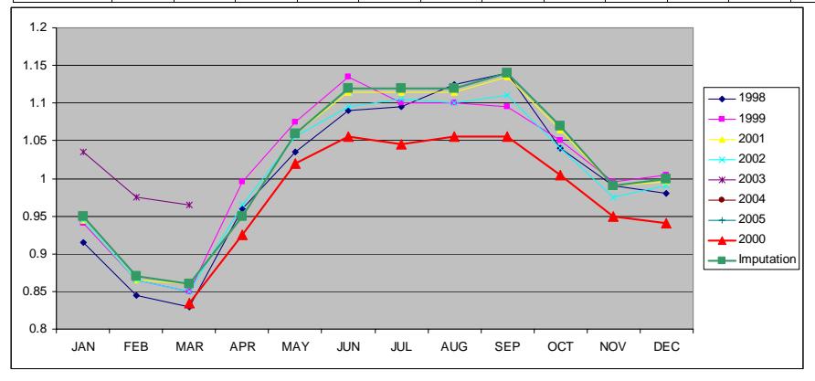
### **B.3 Imputation for Site 030351**
For site 030351, MSFs for April to December are from 2000, MSFs for January to March are borrowed from 2001.
| | JAN | FEB | MAR APR | | MAY JUN | | JUL | AUG | SEP | OCT | NOV | DEC |
|------------|------------|------------------------|-----------------|------------|---------|------|-------|-------|-------|------------------|------------|-------|
| 1998 | | | | | | | | | | | | |
| 1999 | | | | | | | | | | | | |
| | 2001 0.995 | 0.9 | 0.83 | 0.94 | 1.06 | 1.02 | 1.005 | 1 | 1.13 | 1.1 | 1.01 | 1.05 |
| 2002 | | 1.05 0.865 | | 0.83 0.935 | 1.02 | 1.04 | 1 | 1 | 1.175 | | 1.12 1.015 | 1.08 |
| 2003 | | 1.03 0.895 0.855 0.965 | | | 1.005 | 1.04 | 0.985 | 1.025 | | 1.175 1.055 | 0.99 | 1.05 |
| | 2004 1.035 | 0.94 | 0.88 | 0.96 | 1.065 | 1.02 | 0.985 | 1.02 | 1.16 | | 1.03 0.995 | 1.035 |
| | 2005 1.005 | | 0.9 0.895 0.965 | | 1.01 | 1.03 | 0.95 | 1.06 | | 1.125 1.115 | 1.02 | 0.995 |
| | | | | | | | | | | | | |
| 2000 | | | | 0.89 | 1.03 | 0.97 | 0.965 | 0.98 | | 1.07 1.065 0.985 | | 0.965 |
| Imputation | 1 | 0.9 | 0.83 | 0.89 | 1.03 | 0.97 | 0.97 | 0.98 | 1.07 | 1.07 | 0.99 | 0.97 |
| Source | 2001 | 2001 | 2001 | 2000 | 2000 | 2000 | 2000 | 2000 | 2000 | 2000 | 2000 | 2000 |
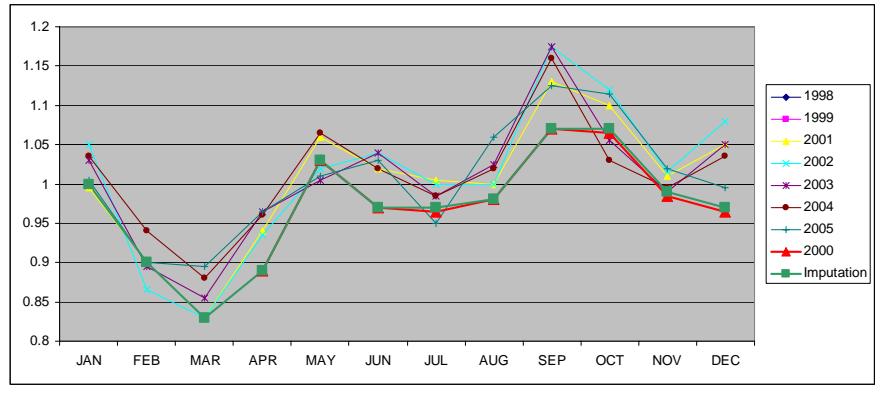
### **B.4 Imputation for Site 040271**
For site 040271, MSFs for all months are borrowed from 2001.
| | JAN | FEB | MAR APR | | MAY JUN | | JUL | AUG | SEP | OCT | NOV | DEC |
|------------|------------|------------------|---------|------------|---------|-------|-------|-------|-------|-------------------|------------|-------|
| 1998 | | 0.94 0.905 0.915 | | 0.92 | | | 1.275 | 1.195 | | 1.185 1.105 1.015 | | 0.96 |
| | 1999 1.055 | 0.98 | 0.97 | 1.03 | | | | | | | | |
| 2001 | | 0.95 0.845 0.895 | | 0.95 | 1.005 | 1.14 | 1.175 | 1.155 | 1.145 | 1.08 | 0.97 | 0.925 |
| 2002 | | 0.94 0.865 | | 0.85 0.915 | 0.98 | 1.135 | 1.155 | 1.12 | 1.12 | | 1.08 0.975 | 0.97 |
| 2003 | 0.93 | 0.87 | 0.86 | 0.94 | 1.005 | 1.125 | 1.195 | 1.15 | 1.135 | | 1.07 0.995 | 0.985 |
| | 2004 0.975 | 0.89 | 0.91 | 0.98 | 1.05 | 1.175 | 1.185 | 1.16 | 1.01 | 0.96 | 0.92 | 0.905 |
| 2005 | 0.9 | 0.85 | 0.86 | 0.92 | 0.96 | 1.085 | 1.12 | 1.125 | 1.155 | | 1.12 1.045 | 0.97 |
| | | | | | | | | | | | | |
| 2000 | | | | 0.875 | 0.93 | 1.075 | 1.09 | 1.065 | 1.035 | 1.03 | 0.93 | 0.87 |
| Imputation | 0.95 | 0.85 | 0.9 | 0.95 | 1.01 | 1.14 | 1.18 | 1.16 | 1.15 | 1.08 | 0.97 | 0.93 |
| Source | 2001 | 2001 | 2001 | 2001 | 2001 | 2001 | 2001 | 2001 | 2001 | 2001 | 2001 | 2001 |
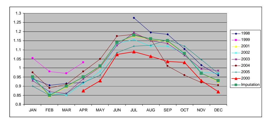
### **B.5 Imputation for Site 090229**
For site 090229, MSFs for all months except July are from 2000. For July, MSF is borrowed from 1999.
| | JAN | FEB | MAR APR | | MAY JUN | | JUL | AUG | SEP | OCT | NOV | DEC |
|------------|-------|-------|---------|-------|---------|-------|-------|-------|-------|-------|-------|-------|
| 1998 | 0.915 | 0.875 | 0.91 | 0.935 | 0.96 | 1.085 | 1.16 | 1.125 | 1.075 | 1.04 | 0.98 | 0.965 |
| 1999 | 0.955 | 0.93 | 0.94 | 0.94 | 0.985 | 1.04 | 1.12 | 1.105 | 1.065 | 1.06 | 1.06 | 1.005 |
| 2001 | 0.955 | 0.895 | 0.9 | 0.945 | 0.995 | 1.08 | 1.145 | 1.055 | 1.05 | 1.03 | 0.96 | |
| 2002 | | 0.91 | 0.92 | 0.93 | 0.96 | 1.085 | 1.125 | 1.08 | | | | |
| 2003 | | | | 0.93 | 0.94 | 1.03 | 1.05 | 1.02 | 0.995 | 0.975 | | |
| 2004 | 0.99 | 0.96 | 0.965 | 0.985 | 1.025 | 1.1 | 1.105 | 1.03 | 1.045 | 0.945 | 0.925 | 0.905 |
| 2005 | 0.955 | 0.915 | 0.94 | 0.95 | 0.985 | 1.1 | 1.105 | 1.05 | 1.08 | 1.035 | 0.96 | 0.915 |
| | | | | | | | | | | | | |
| 2000 | 0.96 | 0.92 | 0.955 | 0.99 | 1.03 | 1.045 | | 1.115 | 1.085 | 1.005 | 0.965 | 0.945 |
| Imputation | 0.96 | 0.92 | 0.96 | 0.99 | 1.03 | 1.05 | 1.12 | 1.12 | 1.09 | 1.01 | 0.97 | 0.95 |
| Source | 2000 | 2000 | 2000 | 2000 | 2000 | 2000 | 1999 | 2000 | 2000 | 2000 | 2000 | 2000 |
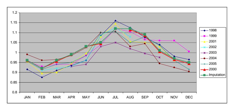
### **B.6 Imputation for Site 120273**
For site 120273, MSFs for all months are borrowed from 2001.
| | JAN | FEB | MAR APR | | MAY JUN | | JUL | AUG | SEP | OCT | NOV | DEC |
|------------|-------|-------|---------|-------|---------|-------|-------|-------|-------|-------|-------|-------|
| 1998 | 0.99 | 0.97 | 0.93 | 0.945 | 0.88 | 1.035 | 1.135 | 1.095 | 1.12 | 1.045 | 1.01 | 0.935 |
| 1999 | 1.07 | 0.99 | 0.935 | 0.94 | 0.99 | 1.115 | 1.075 | 1.04 | 1.015 | 1.035 | 0.965 | 1.01 |
| 2001 | 1.025 | 0.97 | 0.975 | 0.93 | 0.96 | 1.035 | 1.14 | 1.06 | 1.03 | 0.99 | 0.965 | 0.965 |
| 2002 | 1 | 0.93 | 0.905 | 0.92 | 0.945 | 1.08 | 1.105 | 1.12 | 1.09 | 1.005 | 0.955 | 0.99 |
| 2003 | 1.005 | 0.945 | 0.955 | 0.995 | 0.97 | 1.07 | 1.15 | 1.145 | 0.99 | 0.945 | 0.93 | 0.98 |
| 2004 | 1.01 | 0.985 | 0.955 | 0.99 | 0.93 | 1 | 1.105 | 1.15 | 1.075 | 0.95 | 0.965 | 0.98 |
| 2005 | 1.13 | 1.1 | 1.035 | 0.97 | 0.915 | 1.01 | 0.975 | 0.97 | 0.975 | 0.97 | 1 | 0.995 |
| | | | | | | | | | | | | |
| 2000 | | | | | | | | 0.955 | 1.025 | 1.045 | 0.98 | 1.005 |
| Imputation | 1.03 | 0.97 | 0.98 | 0.93 | 0.96 | 1.04 | 1.14 | 1.06 | 1.03 | 0.99 | 0.97 | 0.97 |
| Source | 2001 | 2001 | 2001 | 2001 | 2001 | 2001 | 2001 | 2001 | 2001 | 2001 | 2001 | 2001 |
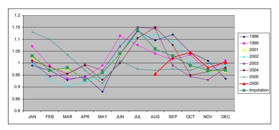
### **B.7 Imputation for Site 130146**
For site 130146, MSFs for all months except June are borrowed from 1999. For June, MSF is estimated as the average of year 1998 to 2005.
| | JAN | FEB | MAR APR | | MAY JUN | | JUL | AUG | SEP | OCT | NOV | DEC |
|------------|-------|-------|---------|-------|---------|-------|-------|-------|-------|-------|-------|-------|
| 1998 | 1.055 | 0.945 | 0.9 | 0.945 | 0.935 | 0.975 | 1.18 | 1.18 | 1.14 | 1.045 | 0.98 | 0.96 |
| 1999 | 0.965 | 0.885 | 0.895 | 0.95 | 0.945 | 1.12 | 1.145 | 1.195 | 1.145 | 1.095 | 1.045 | 1.04 |
| 2001 | 1.005 | 0.9 | 0.905 | 0.935 | 0.96 | 1.055 | 1.175 | 1.14 | 1.16 | 1.03 | 0.96 | 0.935 |
| 2002 | 1.02 | 0.945 | 0.91 | 0.955 | 0.975 | 1.055 | 1.155 | 1.15 | 1.085 | 1.04 | 0.97 | 1.01 |
| 2003 | 0.98 | 0.925 | 0.925 | 0.955 | 0.945 | 1.065 | 1.14 | 1.125 | 1.085 | 1.03 | 0.97 | 0.97 |
| 2004 | 1 | 0.925 | 0.905 | 0.96 | 0.97 | 1.04 | 1.135 | 1.17 | 1.105 | 1.035 | 1.015 | 0.99 |
| 2005 | 0.965 | 0.905 | 0.905 | 0.94 | 0.965 | 1.055 | 1.1 | 1.145 | 1.1 | 1.03 | 1.005 | 0.955 |
| | | | | | | | | | | | | |
| 2000 | 0.98 | 0.88 | 0.875 | | | | 1.15 | 1.14 | 1.08 | 1.01 | 0.95 | 0.93 |
| Imputation | 0.97 | 0.89 | 0.9 | 0.95 | 0.95 | 1.05 | 1.15 | 1.2 | 1.15 | 1.1 | 1.05 | 1.04 |
| Source | 1999 | 1999 | 1999 | 1999 | 1999 | AVG | 1999 | 1999 | 1999 | 1999 | 1999 | 1999 |
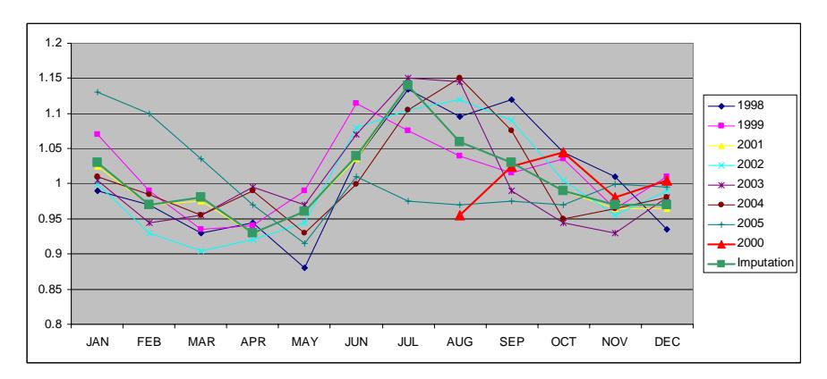
### **B.8 Imputation for Site 140079**
For site 140079, MSFs for all months are borrowed from 1999.
| | JAN | FEB | MAR APR | | MAY JUN | | JUL | AUG | SEP | OCT | NOV | DEC |
|------------|-------|-------|---------|-------|---------|-------|-------|-------|-------|-------|-------|-------|
| 1998 | 0.955 | 0.925 | 0.92 | 0.97 | 1.015 | 1.05 | 1.075 | 1.08 | 1.07 | 1.02 | 0.985 | 0.985 |
| 1999 | 1.05 | 0.905 | 0.935 | 0.95 | 0.995 | 1.045 | 1.075 | 1.085 | 1.005 | 1.03 | 0.99 | 0.98 |
| 2001 | | | | | 1.005 | 1.065 | 1.065 | 1.01 | 0.935 | 0.99 | 0.955 | 0.93 |
| 2002 | 0.97 | 0.905 | 0.905 | 0.945 | 1.005 | 1.06 | 1.075 | 1.05 | 1.055 | 1.04 | 1.005 | 0.98 |
| 2003 | 0.975 | 0.92 | 0.925 | 0.985 | 0.995 | 1.06 | 1.09 | 1.055 | 1.045 | 1.015 | 0.995 | 0.975 |
| 2004 | 0.98 | 0.92 | 0.92 | 0.98 | 1.02 | 1.07 | 1.085 | 1.06 | 1.055 | 1.005 | 0.985 | 0.965 |
| 2005 | 0.96 | 0.91 | 0.92 | 0.95 | 0.99 | 1.04 | 1.075 | 1.08 | 1.075 | 1.045 | 1.005 | 0.97 |
| | | | | | | | | | | | | |
| 2000 | 1.03 | 0.95 | 0.935 | 1.05 | 1.075 | 1.03 | 1.07 | | | | | |
| Imputation | 1.05 | 0.91 | 0.94 | 0.95 | 1 | 1.05 | 1.08 | 1.09 | 1.01 | 1.03 | 0.99 | 0.98 |
| Source | 1999 | 1999 | 1999 | 1999 | 1999 | 1999 | 1999 | 1999 | 1999 | 1999 | 1999 | 1999 |
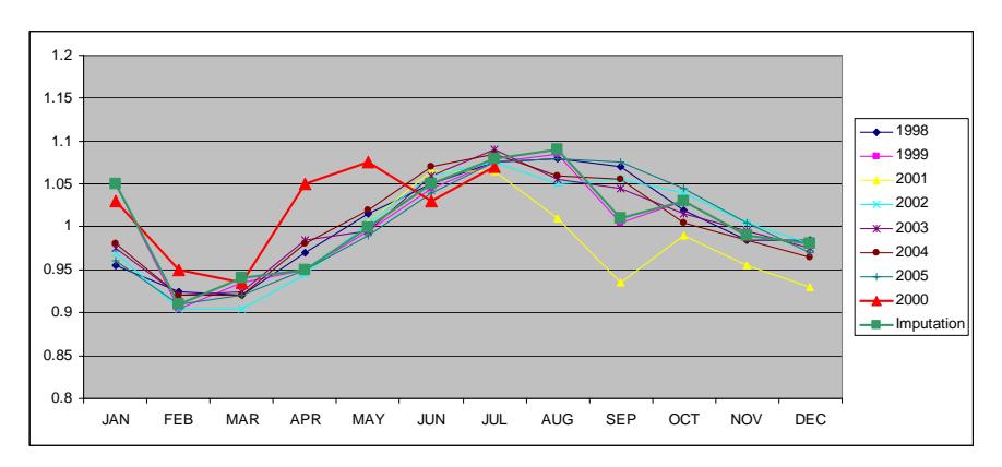
### **B.9 Imputation for Site 290269**
For site 269904, MSFs for all months are borrowed from 2001
| | JAN | FEB | MAR APR | | MAY JUN | | JUL | AUG | SEP | OCT | NOV | DEC |
|------------|-------|-------|---------|-------|---------|-------|-------|-------|------|-------|-------|-------|
| 1998 | 1 | | | | | | | | | | | |
| 1999 | 1.135 | 1.1 | 1.01 | 1.1 | 1.02 | 0.935 | 0.895 | 0.955 | 1.09 | 1.07 | | |
| 2001 | 1.175 | 1.08 | 0.955 | 0.975 | 1.01 | 0.91 | 0.87 | 1.005 | 1.06 | 1.03 | 1.020 | 1.105 |
| 2002 | 1.175 | 1.055 | 0.905 | 0.960 | 0.975 | 0.91 | 0.895 | 1 | 1.1 | 1.06 | 1.055 | 1.105 |
| 2003 | 1.16 | 1.08 | 0.93 | 0.995 | 0.94 | 0.915 | 0.865 | 0.985 | 1.08 | 1.02 | 0.955 | 1.115 |
| 2004 | 1.14 | 1.075 | 0.935 | 0.955 | 1.04 | 0.94 | 0.88 | 1.025 | 1.09 | 0.995 | 1.02 | 1.075 |
| 2005 | 1.13 | 1.05 | 0.915 | 0.935 | 0.975 | 0.895 | 0.845 | 1.01 | 1.09 | 1.015 | 1.06 | 1.095 |
| | | | | | | | | | | | | |
| 2000 | | | | | | | | | 0.78 | 1.02 | 1.005 | 0.955 |
| Imputation | 1.18 | 1.08 | 0.96 | 0.98 | 1.01 | 0.91 | 0.87 | 1.01 | 1.06 | 1.03 | 1.02 | 1.11 |
| Source | 2001 | 2001 | 2001 | 2001 | 2001 | 2001 | 2001 | 2001 | 2001 | 2001 | 2001 | 2001 |
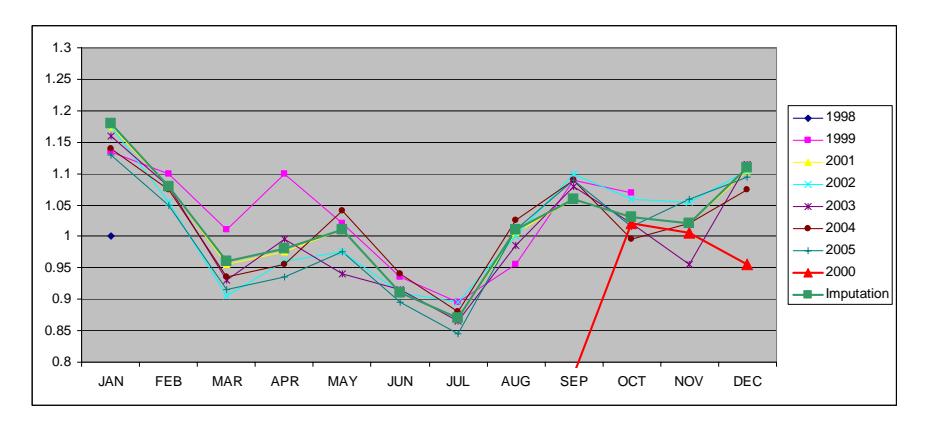
### **B.10 Imputation for Site 299936**
For site 299936, MSFs for all months are borrowed from 2001
| | JAN | FEB | MAR APR | | MAY JUN | | JUL | AUG | SEP | OCT | NOV | DEC |
|------------|-------|-------|---------|-------|---------|-------|-------|-------|-------|-------|-------|-------|
| 1998 | 1.22 | 1.035 | 1.025 | | | 0.91 | 0.87 | 0.98 | 1.2 | 1.01 | | |
| 1999 | | | | 0.85 | 1.055 | 0.925 | 0.81 | 0.98 | 1.08 | 1.05 | 1.065 | 1.135 |
| 2001 | 1.19 | 1.085 | 0.975 | 0.98 | 1.015 | 0.93 | 0.88 | 0.945 | 1.04 | 1 | 1.02 | 1.175 |
| 2002 | 1.155 | 0.985 | 0.895 | 0.93 | 0.98 | 0.875 | 1.05 | 1.035 | 1.07 | 1.01 | 1.05 | 1.135 |
| 2003 | 1.185 | 1.06 | 1.02 | 0.91 | 0.975 | 0.915 | 0.86 | 0.95 | 1.08 | 0.995 | 1.035 | 1.085 |
| 2004 | 1.185 | 1.07 | 0.955 | 0.96 | 1.005 | 0.925 | 0.875 | 1 | 1.125 | 0.985 | 1.07 | 1.095 |
| 2005 | 1.12 | 1.05 | 0.94 | 0.975 | 0.99 | 0.91 | 0.88 | 1.005 | 1.09 | 1.02 | 1.075 | 1.1 |
| | | | | | | | | | | | | |
| 2000 | 1.135 | 1.13 | | | 0.985 | 0.92 | 0.87 | 0.955 | 1.07 | 0.995 | 1.04 | 1.165 |
| Imputation | 1.19 | 1.09 | 0.98 | 0.98 | 1.02 | 0.93 | 0.88 | 0.95 | 1.04 | 1 | 1.02 | 1.18 |
| Source | 2001 | 2001 | 2001 | 2001 | 2001 | 2001 | 2001 | 2001 | 2001 | 2001 | 2001 | 2001 |
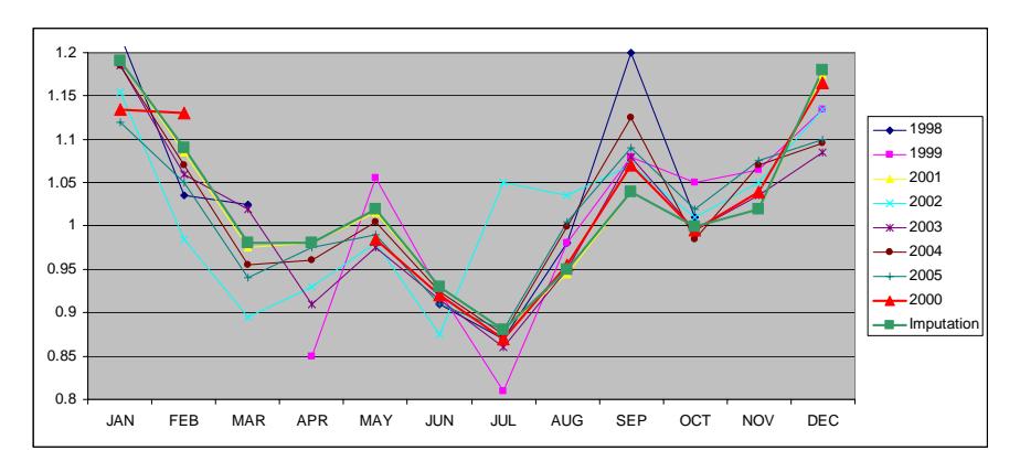
### **B.11 Imputation for Site 300234**
For site 300234, MSFs for all months are borrowed from 1999
| | JAN | FEB | MAR APR | | MAY JUN | | JUL | AUG | SEP | OCT | NOV | DEC |
|------------|-------|-------|---------|-------|---------|-------|-------|-------|-------|-------|-------|-------|
| 1998 | 1.085 | 1.015 | 0.975 | 1.015 | 0.98 | 0.965 | 0.995 | 1.015 | 1.02 | 0.995 | 1.02 | 0.995 |
| 1999 | 1.04 | 0.975 | 0.93 | 0.985 | 1.035 | 0.985 | 0.995 | 1.045 | 1.085 | 1.03 | 1.015 | 0.995 |
| 2001 | 1.015 | 0.98 | 0.96 | 0.97 | 0.98 | 0.965 | 0.995 | 1 | 1.055 | 1.05 | 1.05 | 1 |
| 2002 | 1.05 | 0.98 | 0.95 | 0.985 | 0.98 | 0.935 | 0.965 | 0.995 | 1.135 | 1.095 | 0.98 | 1.005 |
| 2003 | 1.035 | 0.995 | 0.995 | 0.995 | 0.965 | 0.985 | 0.995 | 1.005 | 1.015 | 0.995 | 1 | 1.025 |
| 2004 | 1.185 | 1.08 | 0.96 | 0.985 | 1.005 | 0.995 | 0.985 | 1.01 | 0.98 | 0.975 | 1 | 0.95 |
| 2005 | 0.99 | 0.965 | 0.96 | 0.975 | 0.98 | 0.985 | 1.01 | 1.045 | 1.07 | 1.03 | 1.03 | 0.985 |
| | | | | | | | | | | | | |
| 2000 | 1.06 | 0.95 | 0.925 | | | | 0.95 | 1.03 | 1.035 | 1.01 | 0.99 | 0.99 |
| Imputation | 1.04 | 0.98 | 0.93 | 0.99 | 1.04 | 0.99 | 1 | 1.05 | 1.09 | 1.03 | 1.02 | 1 |
| Source | 1999 | 1999 | 1999 | 1999 | 1999 | 1999 | 1999 | 1999 | 1999 | 1999 | 1999 | 1999 |
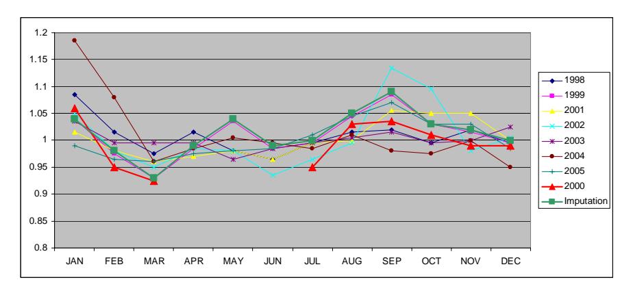
### **B.12 Imputation for Site 479944**
For site 479944, MSFs for all months are borrowed from 1999
| | JAN | FEB | MAR APR | | MAY JUN | | JUL | AUG | SEP | OCT | NOV | DEC |
|------------|-------|------|---------|-------|---------|-------|-------|-------|-------|-------|-------|-------|
| 1998 | | | | | | | | | 1.035 | 0.995 | 0.995 | 0.995 |
| 1999 | 1.07 | 1 | 0.985 | 0.97 | 0.97 | 0.975 | 0.99 | 1 | 1.05 | 1 | 1.005 | 1.015 |
| 2001 | 1.07 | 1.01 | 1.02 | 0.95 | 0.935 | 0.955 | 0.925 | 1.065 | 1.07 | 1.045 | 1.015 | 1.025 |
| 2002 | 1.05 | 1.01 | 0.985 | 0.96 | 0.955 | 0.945 | 0.975 | 0.975 | 1.07 | 1.05 | 1.05 | 1.055 |
| 2003 | 1.09 | 1.04 | 1.015 | 0.97 | 0.955 | 0.965 | 0.99 | 1.02 | 1.005 | 0.99 | 0.98 | 0.99 |
| 2004 | 1.07 | 1.04 | 1.01 | 0.935 | 0.99 | 0.99 | 0.945 | 1 | | 0.98 | 1.035 | 1.07 |
| 2005 | 1.045 | 1.02 | 1.01 | 0.95 | 0.96 | 0.96 | 0.935 | 1.015 | 1.025 | 1.01 | 0.995 | 1.075 |
| | | | | | | | | | | | | |
| 2000 | 1.04 | 1.01 | 1 | 0.95 | 0.965 | 0.98 | 1.015 | 1.055 | 1.15 | | | |
| Imputation | 1.07 | 1 | 0.99 | 0.97 | 0.97 | 0.98 | 0.99 | 1 | 1.05 | 1 | 1.01 | 1.02 |
| Source | 1999 | 1999 | 1999 | 1999 | 1999 | 1999 | 1999 | 1999 | 1999 | 1999 | 1999 | 1999 |
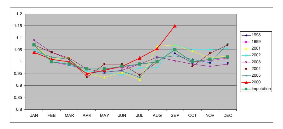
### **B.13 Imputation for Site 480348**
For site 480348, MSFs for May to December are from 2000. For January to April, MSFs are estimated as the average of year 2002 to 2005.
| | JAN | FEB | MAR APR | | MAY JUN | | JUL | AUG | SEP | OCT | NOV | DEC |
|------------|-------|-------|---------|-------|---------|-------|-------|-------|-------|-------|-------|-------|
| 1998 | | | | | | | | | | | | |
| 1999 | | | | | | | | | | | | |
| 2001 | 1.06 | 1.015 | 0.945 | | | | | | | | | |
| 2002 | 1.175 | 1.065 | 1.005 | 0.98 | 0.94 | 0.915 | 0.925 | 0.975 | 1.03 | 1.035 | 1.07 | 1.065 |
| 2003 | 1.12 | 1.095 | 1.02 | 1.01 | 0.95 | 0.935 | 0.915 | 0.965 | 1.03 | 0.995 | 1.07 | 1.06 |
| 2004 | 1.135 | 1.15 | 0.995 | 0.995 | 0.995 | 0.985 | 0.93 | 1.02 | 0.985 | 0.93 | | 0.97 |
| 2005 | 1.03 | 1.015 | 0.975 | 1 | 0.95 | 0.945 | 0.91 | 0.98 | 1.04 | 1.04 | 1.075 | 1.09 |
| | | | | | | | | | | | | |
| 2000 | | | | | 0.96 | 0.935 | 0.93 | 0.99 | 1.055 | 1.03 | 1.065 | 1.115 |
| Imputation | 1.12 | 1.08 | 1 | 1 | 0.96 | 0.94 | 0.93 | 0.99 | 1.06 | 1.03 | 1.07 | 1.12 |
| Source | AVG | AVG | AVG | AVG | 2000 | 2000 | 2000 | 2000 | 2000 | 2000 | 2000 | 2000 |
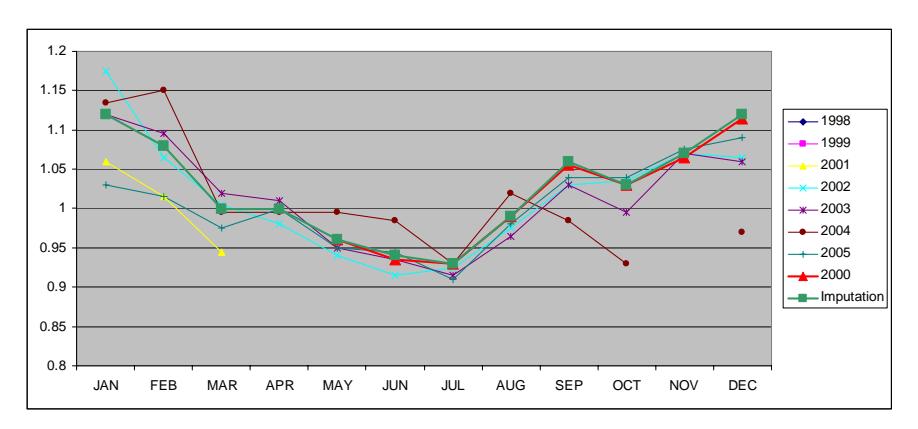
### **B.14 Imputation for Site 540245**
For site 540245, MSFs for all months except August and September are from 2000. For August and September, MSFs are borrowed from 1999.
| | JAN | FEB | MAR APR | | MAY JUN | | JUL | AUG | SEP | OCT | NOV | DEC |
|------------|-------|-------|---------|-------|---------|-------|-------|-------|-------|-------|-------|------|
| 1998 | 1.05 | 1.02 | 0.99 | 0.975 | 0.96 | 0.985 | 1.035 | 1.015 | 1.025 | 1 | 0.96 | 0.98 |
| 1999 | 1.045 | 0.995 | 0.955 | 0.95 | 0.985 | 0.98 | 0.995 | 0.99 | 1.01 | 1.065 | 1.035 | 1.02 |
| 2001 | 1.04 | 1.02 | 1.015 | 0.96 | 1 | 0.975 | 1.005 | 1.02 | 1.01 | 0.99 | 1 | 0.98 |
| 2002 | 1.07 | 0.995 | 0.97 | 1.015 | 0.995 | 1.005 | 1.015 | 1.015 | 1.025 | 1.005 | 0.935 | 0.94 |
| 2003 | 1.015 | 1.045 | 0.99 | 0.985 | 0.95 | 1.015 | 1.005 | 1 | 1 | 1 | 0.98 | 1.01 |
| 2004 | 1.03 | 1.06 | 0.98 | 0.98 | 0.965 | 1.03 | 0.96 | 1.035 | 1.01 | 1 | 0.985 | 0.99 |
| 2005 | 0.975 | 0.985 | 1 | 0.995 | 0.96 | 0.965 | 0.985 | 1.02 | 1.075 | 1.05 | 1.005 | 1 |
| | | | | | | | | | | | | |
| 2000 | 1.015 | 0.98 | 0.97 | 0.95 | 0.98 | 1.03 | 1.015 | | | 1.045 | 1.025 | 1 |
| Imputation | 1.02 | 0.98 | 0.97 | 0.95 | 0.98 | 1.03 | 1.02 | 0.99 | 1.01 | 1.05 | 1.03 | 1 |
| Source | 2000 | 2000 | 2000 | 2000 | 2000 | 2000 | 2000 | 1999 | 1999 | 2000 | 2000 | 2000 |
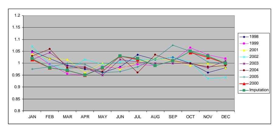
### **B.15 Imputation for Site 550211**
For site 550211, MSFs for all months are estimated as the average of all the available data from year 1998 to 2005.
| | JAN | FEB | MAR APR | | MAY JUN | | JUL | AUG | SEP | OCT | NOV | DEC |
|------------|-------|-------|---------|-------|---------|-------|-------|-------|-------|-------|-------|-------|
| 1998 | 1.05 | 1.015 | 0.99 | 0.96 | 0.955 | 1.02 | 1.015 | 0.995 | 1.02 | 0.985 | | |
| 1999 | | | 1.01 | 0.98 | 1 | 1.055 | | 1.02 | | 1.01 | | |
| 2001 | 1.065 | 1.005 | 0.995 | 0.965 | 0.99 | | | | | | | |
| 2002 | | | 0.965 | 0.955 | 0.96 | 1.02 | 1.015 | 1.015 | 1.01 | 1.01 | 1.005 | 1.025 |
| 2003 | 1.035 | 0.985 | 1 | 0.98 | 0.955 | 1.04 | 1.03 | 1.005 | 0.985 | 1 | 0.99 | 1.015 |
| 2004 | 1.04 | 1.04 | 0.99 | 0.96 | 0.955 | 1.02 | 1.015 | 1 | 0.995 | 0.99 | 1 | 1 |
| 2005 | 0.995 | 0.98 | 0.97 | 0.96 | 0.955 | 1.01 | 0.99 | 1.015 | 1.03 | 1.035 | 1.035 | 1.04 |
| | | | | | | | | | | | | |
| 2000 | | | | | | 1.065 | 1.035 | 1.005 | 0.99 | 0.99 | 1.005 | 0.985 |
| Imputation | 1.04 | 1.01 | 0.99 | 0.97 | 0.97 | 1.03 | 1.01 | 1.01 | 1.01 | 1.01 | 1.01 | 1.02 |
| Source | AVG | AVG | AVG | AVG | AVG | AVG | AVG | AVG | AVG | AVG | AVG | AVG |
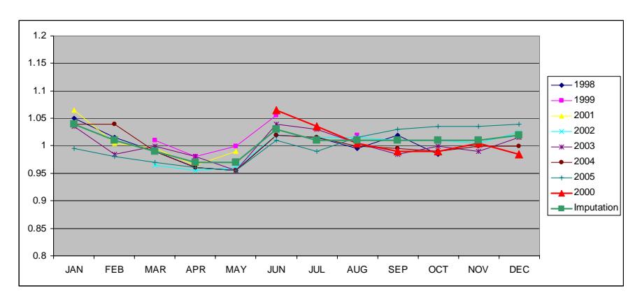
### **B.16 Imputation for Site 550349**
For site 550349, MSFs for all months are estimated as the average of year 2002 to 2005.
| | JAN | FEB | MAR APR | | MAY JUN | | JUL | AUG | SEP | OCT | NOV | DEC |
|------------|-------|------|---------|-------|---------|-------|-------|-------|-------|-------|-------|-------|
| 1998 | | | | | | | | | | | | |
| 1999 | | | | | | | | | | | | |
| 2001 | 1.18 | 1.16 | 1.22 | 1.17 | 1.21 | 0.98 | 0.99 | 0.915 | 0.97 | 0.93 | 0.91 | 0.9 |
| 2002 | 1.115 | 1.12 | 0.99 | 0.975 | 0.985 | 0.98 | 0.955 | 0.965 | 1.04 | 0.98 | 1.005 | 0.985 |
| 2003 | 1.11 | 1.04 | 1 | 1.005 | 0.96 | 0.955 | 0.955 | 0.97 | 1.04 | 0.995 | 1.005 | 1.01 |
| 2004 | 1.065 | 1.01 | 1 | 0.96 | 0.985 | 0.985 | 0.965 | 1.03 | 1.06 | 0.97 | 1.02 | 1.005 |
| 2005 | 1.045 | 1.01 | 0.98 | 0.935 | 0.995 | 0.98 | 0.94 | 1.005 | 1.045 | 1.015 | 1.01 | 1.02 |
| | | | | | | | | | | | | |
| 2000 | | | | | | | 0.95 | 1.005 | 1.04 | 0.985 | 1.04 | 0.98 |
| Imputation | 1.08 | 1.05 | 0.99 | 0.97 | 0.98 | 0.98 | 0.95 | 0.99 | 1.05 | 0.99 | 1.01 | 1.01 |
| Source | AVG | AVG | AVG | AVG | AVG | AVG | AVG | AVG | AVG | AVG | AVG | AVG |
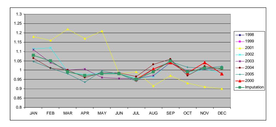
### **B.17 Imputation for Site 560301**
For site 560301, MSFs for all months except December are borrowed from 1999. For December, MSF is estimated as the average of year 1998, 2001 to 2005.
| | JAN | FEB | MAR APR | | MAY JUN | | JUL | AUG | SEP | OCT | NOV | DEC |
|------------|-------|-------|---------|-------|---------|-------|-------|-------|-------|-------|-------|-------|
| 1998 | 1.03 | 1.025 | 0.98 | 0.975 | 0.965 | 0.925 | 0.92 | 1.04 | 1.08 | 1.02 | 1.005 | 1.03 |
| 1999 | 1.06 | 1.025 | 0.985 | 0.955 | 0.98 | 0.94 | 0.95 | 0.935 | 1.045 | 1.01 | 1.015 | 1.105 |
| 2001 | 1.14 | 1.035 | 1.01 | 0.975 | 0.98 | 0.945 | 0.95 | 0.985 | 1.04 | 1 | 1 | 1.01 |
| 2002 | 1.06 | 1.005 | 1 | 1.005 | 0.99 | 0.975 | 0.96 | 1 | 1.025 | 0.975 | 1.01 | 1.025 |
| 2003 | 1.08 | 1.04 | 0.995 | 0.995 | 0.95 | 0.89 | 0.965 | 1.015 | 1.025 | 0.985 | 1 | 1.02 |
| 2004 | 1.085 | 1.05 | 0.98 | 0.955 | 1.005 | 0.935 | 0.955 | 1.03 | 1.035 | 0.99 | 1.015 | 1.015 |
| 2005 | 1.06 | 1.025 | 0.98 | 0.96 | 0.96 | 0.945 | 0.95 | 1.02 | 1.06 | 1.04 | 1.02 | 1.01 |
| | | | | | | | | | | | | |
| 2000 | 1.175 | | | | | | | | 0.915 | 0.9 | 0.965 | 0.95 |
| Imputation | 1.06 | 1.03 | 0.99 | 0.96 | 0.98 | 0.94 | 0.95 | 0.94 | 1.05 | 1.01 | 1.02 | 1.02 |
| Source | 1999 | 1999 | 1999 | 1999 | 1999 | 1999 | 1999 | 1999 | 1999 | 1999 | 1999 | AVG |
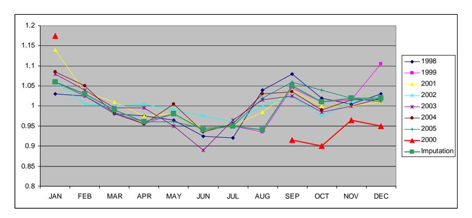
### **B.18 Imputation for Site 580251**
For site 580251, MSFs for all months except February are from 2000. For February, MSF is borrowed from 1999.
| | JAN | FEB | MAR APR | | MAY JUN | | JUL | AUG | SEP | OCT | NOV | DEC |
|------------|-------|-------|---------|-------|---------|-------|-------|-------|-------|-------|-------|-------|
| 1998 | 1.05 | 1.05 | 1.055 | 0.955 | 0.98 | 0.96 | 1 | 0.97 | 0.995 | 1.005 | 1.02 | 0.98 |
| 1999 | 1.13 | 1.025 | 0.97 | 0.985 | 1 | 0.965 | 0.945 | 0.915 | 0.99 | 0.99 | 1.005 | 1 |
| 2001 | 1.04 | 0.995 | 1.02 | 1.005 | 1.005 | 0.985 | 1.005 | 1.01 | 0.99 | 0.99 | 0.975 | 0.98 |
| 2002 | 1.005 | 1.03 | 0.965 | 0.975 | 0.975 | 0.97 | 0.95 | 0.975 | 1.03 | 1.065 | 1.045 | 1.085 |
| 2003 | 1.045 | 1.065 | 1.005 | 0.985 | 0.95 | 0.975 | 0.98 | 1.025 | 1.015 | 0.985 | 0.985 | 1.005 |
| 2004 | 1.08 | 1.09 | 0.995 | 1 | 0.98 | 1.005 | 0.975 | 1.03 | | | 0.865 | |
| 2005 | 1.035 | 1.015 | 1 | 0.97 | | 0.935 | 0.94 | 0.975 | 1.04 | 1.04 | 1.025 | 1.05 |
| | | | | | | | | | | | | |
| 2000 | 1.02 | | 0.955 | 0.935 | 0.99 | 0.93 | 0.97 | 1.05 | 1.095 | 1.01 | 1.02 | 1.005 |
| Imputation | 1.02 | 1.03 | 0.96 | 0.94 | 0.99 | 0.93 | 0.97 | 1.05 | 1.1 | 1.01 | 1.02 | 1.01 |
| Source | 2000 | 1999 | 2000 | 2000 | 2000 | 2000 | 2000 | 2000 | 2000 | 2000 | 2000 | 2000 |
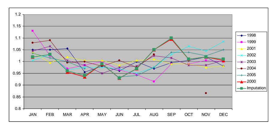
### **B.19 Imputation for Site 599946**
For site 599946, MSFs for all months are estimated as the average of year from 2001 to 2005.
| | JAN | FEB | MAR APR | | MAY JUN | | JUL | AUG | SEP | OCT | NOV | DEC |
|------------|-------|-------|---------|-------|---------|-------|-------|-------|-------|-------|-------|-------|
| 1998 | | | | | | | | 0.925 | 1.03 | 1 | 0.995 | 0.99 |
| 1999 | 1.245 | 1.15 | 1.11 | 1.06 | 1.05 | 1.01 | 0.96 | 0.94 | 0.91 | 0.885 | 0.88 | 0.91 |
| 2001 | 1 | 0.985 | 0.99 | 0.92 | 0.945 | 0.99 | 1.005 | 1.015 | 1.05 | 1.025 | 1.06 | 1.07 |
| 2002 | 1.095 | 1.065 | 1.005 | 0.935 | 0.945 | 1 | 0.98 | 0.97 | 1.01 | 0.99 | 1.03 | 1.115 |
| 2003 | | 0.995 | 0.99 | 0.94 | 0.955 | 1.025 | 1.04 | 1.025 | 1.02 | 0.92 | 1.035 | 1.155 |
| 2004 | 1.095 | 1.055 | 0.935 | 0.955 | 0.91 | 0.99 | 1.01 | 1 | 1.025 | 0.99 | 1.06 | 1.135 |
| 2005 | 1.04 | 1.02 | 1 | 0.93 | 0.915 | 1.03 | 0.95 | 0.99 | 1.085 | 1.01 | 1.04 | 1.025 |
| | | | | | | | | | | | | |
| 2000 | 0.93 | 0.88 | 0.88 | 0.96 | 0.96 | 1.035 | 1.09 | 1.125 | 1.18 | | 0.98 | 1.315 |
| Imputation | 1.06 | 1.02 | 0.98 | 0.94 | 0.93 | 1.01 | 1 | 1 | 1.04 | 0.99 | 1.05 | 1.1 |
| Source | AVG | AVG | AVG | AVG | AVG | AVG | AVG | AVG | AVG | AVG | AVG | AVG |
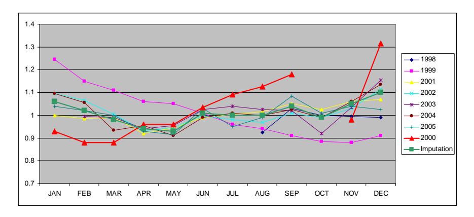
### **B.20 Imputation for Site 609938**
For site 609938, MSFs for all months are borrowed from 1999.
| | JAN | FEB | MAR APR | | MAY JUN | | JUL | AUG | SEP | OCT | NOV | DEC |
|------------|-------|-------|---------|------|---------|-------|-------|-------|------|-------|-------|-------|
| 1998 | 1.215 | 1.09 | 1.045 | 1.01 | 0.915 | 0.86 | 0.86 | 0.935 | 1.04 | 1.06 | 1.14 | 1.17 |
| 1999 | 1.245 | 1.14 | 1.02 | 1 | 0.955 | 0.885 | 0.835 | 0.925 | 1.01 | 1.015 | 1.075 | 1.135 |
| 2001 | | | | | | | | | | | | |
| 2002 | | | | | | | | | | | | |
| 2003 | | | | | | | | | | | | |
| 2004 | | | | | | | | | | | | |
| 2005 | | | | | | | | | | | | |
| | | | | | | | | | | | | |
| 2000 | 1.27 | 1.085 | 0.97 | 1 | 0.98 | | | | | | | |
| Imputation | 1.25 | 1.14 | 1.02 | 1 | 0.96 | 0.89 | 0.84 | 0.93 | 1.01 | 1.02 | 1.08 | 1.14 |
| Source | 1999 | 1999 | 1999 | 1999 | 1999 | 1999 | 1999 | 1999 | 1999 | 1999 | 1999 | 1999 |
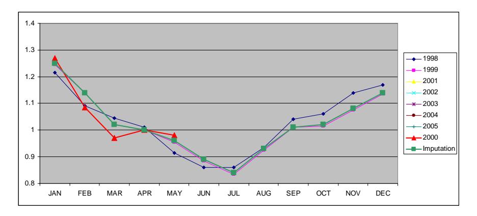
### **B.21 Imputation for Site 700134**
For site 700134, MSFs for all months except December are from 2000. For December, MSF is borrowed from 1999.
| | JAN | FEB | MAR APR | | MAY JUN | | JUL | AUG | SEP | OCT | NOV | DEC |
|------------|-------|-------|---------|-------|---------|-------|-------|-------|-------|-------|-------|-------|
| 1998 | 1 | 1 | | | | | | | | | | |
| 1999 | | 0.985 | 0.93 | 1 | 1.03 | 1.005 | 0.95 | 0.99 | 1.11 | 1.04 | 1.02 | 1.06 |
| 2001 | 1.02 | 0.96 | 0.89 | 0.96 | 1.015 | 1.005 | 0.98 | 1.035 | 1.095 | 1.05 | 0.98 | 1.01 |
| 2002 | 1.09 | 0.995 | 0.865 | 0.985 | 1.04 | 1.01 | | 1.035 | | 1.04 | 1.035 | 1.045 |
| 2003 | 1.03 | 0.98 | 0.88 | 0.95 | 0.985 | 0.985 | 0.985 | 1.12 | 1.19 | 1.095 | 1.045 | 1.015 |
| 2004 | 1.065 | 0.98 | 0.9 | 0.965 | 1.04 | 1.02 | 0.98 | 1.055 | 1.115 | 1.005 | 0.995 | 1.025 |
| 2005 | 1.005 | 0.955 | 0.87 | 0.96 | 1.015 | 0.96 | 0.895 | 1.045 | 1.145 | 1.14 | 1.015 | 1.02 |
| | | | | | | | | | | | | |
| 2000 | 1.035 | 0.95 | 0.905 | 0.98 | 1.025 | 1.01 | 0.965 | 0.995 | 1.13 | 1.035 | 0.98 | |
| Imputation | 1.04 | 0.95 | 0.91 | 0.98 | 1.03 | 1.01 | 0.97 | 1 | 1.13 | 1.04 | 0.98 | 1.06 |
| Source | 2000 | 2000 | 2000 | 2000 | 2000 | 2000 | 2000 | 2000 | 2000 | 2000 | 2000 | 1999 |
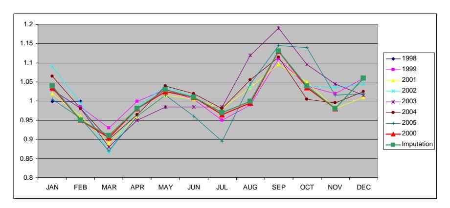
# **B.22 Imputation for Site 700223**
For site 700234, MSFs for all months are borrowed from 1999.
| | JAN | FEB | MAR APR | | MAY JUN | | JUL | AUG | SEP | OCT | NOV | DEC |
|------------|-------|-------|---------|-------|---------|-------|-------|-------|-------|-------|-------|-------|
| 1998 | 1.07 | 0.94 | 0.88 | | | | 0.945 | 0.975 | 1.11 | 1.01 | 1.03 | 1.09 |
| 1999 | 1.11 | 0.95 | 0.905 | 0.98 | 1.05 | 1 | 0.915 | 1 | 1.15 | 1.005 | 1.035 | 1.1 |
| 2001 | 1.065 | 0.92 | 0.835 | 0.885 | 1.01 | 0.945 | 0.885 | 0.94 | 1.285 | 1.175 | 1.13 | 1.24 |
| 2002 | 1.18 | 0.975 | 0.88 | 0.88 | 1.07 | 0.995 | | | | | | |
| 2003 | 1.1 | 0.98 | 0.895 | 0.92 | 1.05 | 0.965 | 0.91 | 0.975 | 1.145 | 1.05 | 1.045 | 1.075 |
| 2004 | 1.095 | 0.91 | 0.88 | 0.91 | 1.03 | 1.03 | | 1 | 1.185 | 1.02 | 1.025 | 1.075 |
| 2005 | 1.065 | 0.945 | 0.865 | 0.945 | 0.995 | 0.96 | 0.885 | 0.96 | 1.18 | 1.07 | 1.055 | 1.105 |
| | | | | | | | | | | | | |
| 2000 | 1.06 | 0.97 | 0.855 | 0.95 | 1.03 | 0.985 | | | 1.08 | 1.02 | 1.06 | 1.065 |
| Imputation | 1.11 | 0.95 | 0.91 | 0.98 | 1.05 | 1 | 0.92 | 1 | 1.15 | 1.01 | 1.04 | 1.1 |
| Source | 1999 | 1999 | 1999 | 1999 | 1999 | 1999 | 1999 | 1999 | 1999 | 1999 | 1999 | 1999 |
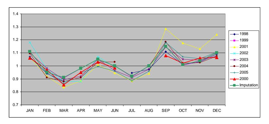
# **B.23 Imputation for Site 740047**
For site 740047, MSFs for all months except June, September, and October, are borrowed from 2001. For June, September, and October, MSFs are estimated as the average of all available data from year 1998 to 2004.
| | JAN | FEB | MAR APR | | MAY JUN | | JUL | AUG | SEP | OCT | NOV | DEC |
|------------|-------|-------|---------|-------|---------|-------|-------|-------|-------|-------|-------|-------|
| 1998 | 1.105 | 1.035 | 1.005 | 1.025 | 0.99 | 0.965 | 0.97 | 1.01 | 1.01 | 0.955 | 1.005 | 1 |
| 1999 | | 1.03 | 1.015 | 1.03 | 1 | 0.97 | 0.965 | 0.96 | | | | |
| 2001 | 1.08 | 1.065 | 1.015 | 0.955 | 0.96 | 0.88 | 0.96 | 0.985 | 1.075 | 1.045 | 1.005 | 1 |
| 2002 | 1.115 | 1.045 | 0.98 | 0.955 | 0.98 | 0.97 | 0.96 | 0.99 | 1.025 | 0.99 | 1 | 1.015 |
| 2003 | 1.075 | 1.04 | 1.015 | 0.975 | 0.97 | 0.955 | 0.965 | 0.995 | 1.02 | 0.98 | 1.03 | 1.02 |
| 2004 | 1.05 | 1.03 | 1 | 0.96 | 0.985 | 0.97 | 0.95 | 1.055 | 1.04 | 0.97 | 1.005 | 1 |
| 2005 | 1.03 | 1.005 | 0.965 | | | | | | | | | |
| | | | | | | | | | | | | |
| 2000 | | | | | 0.97 | 0.96 | 0.915 | 1.01 | 1.055 | 1.005 | 1.045 | 1.02 |
| Imputation | 1.08 | 1.07 | 1.02 | 0.96 | 0.96 | 0.97 | 0.96 | 0.99 | 1.02 | 0.97 | 1.01 | 1 |
| Source | 2001 | 2001 | 2001 | 2001 | 2001 | AVG | 2001 | 2001 | AVG | AVG | 2001 | 2001 |
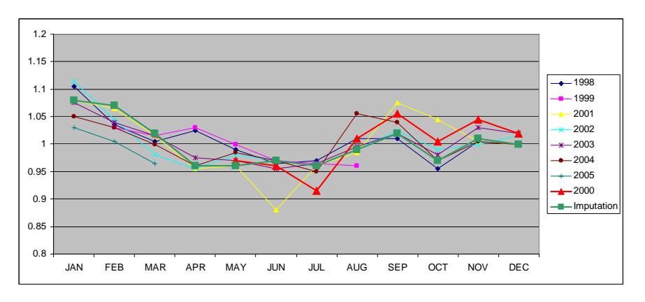
# **B.24 Imputation for Site 750104**
For site 750104, MSFs for all months except May, and June are borrowed from 1999. For May, and June, MSFs are estimated as the average of all available data from year 1998 to 2005.
| | JAN | FEB | MAR APR | | MAY JUN | | JUL | AUG | SEP | OCT | NOV | DEC |
|------------|-------|-------|---------|-------|---------|-------|-------|-------|-------|-------|-------|-------|
| 1998 | 1.05 | 1.015 | 0.985 | 0.99 | 1.01 | 1.005 | 1.04 | 0.96 | 0.87 | 0.9 | 1.035 | 1.04 |
| 1999 | 1.045 | 1 | 0.975 | 0.965 | 1.015 | 1.06 | 0.965 | 0.975 | 0.995 | 1 | 1 | 1 |
| 2001 | 1.035 | 0.945 | 0.935 | 0.965 | 0.985 | 0.97 | 0.99 | 1.045 | 1.04 | 1.045 | 1.04 | 1.01 |
| 2002 | 1.04 | 0.98 | 0.96 | 0.99 | 0.99 | 1.02 | 1 | 1 | 1.01 | 1 | 1 | 1.025 |
| 2003 | 1.065 | 1.05 | 0.96 | 0.98 | 0.985 | 1 | 0.99 | 1.005 | 1.015 | 1 | 1.015 | 1.005 |
| 2004 | 1.03 | 0.985 | 0.96 | 0.98 | 1 | 1.01 | 0.98 | 1.01 | 1.055 | 1 | 1.005 | 1.015 |
| 2005 | 1.02 | 0.985 | 0.975 | 0.98 | 0.985 | 1.005 | 0.97 | 0.995 | 1.035 | 1.025 | 1.03 | 1.015 |
| | | | | | | | | | | | | |
| 2000 | 1.05 | 1.015 | 0.945 | | | | | | | | 0.985 | 1.01 |
| Imputation | 1.05 | 1 | 0.98 | 0.97 | 1 | 1 | 0.97 | 0.98 | 1 | 1 | 1 | 1 |
| Source | 1999 | 1999 | 1999 | 1999 | AVG | AVG | 1999 | 1999 | 1999 | 1999 | 1999 | 1999 |
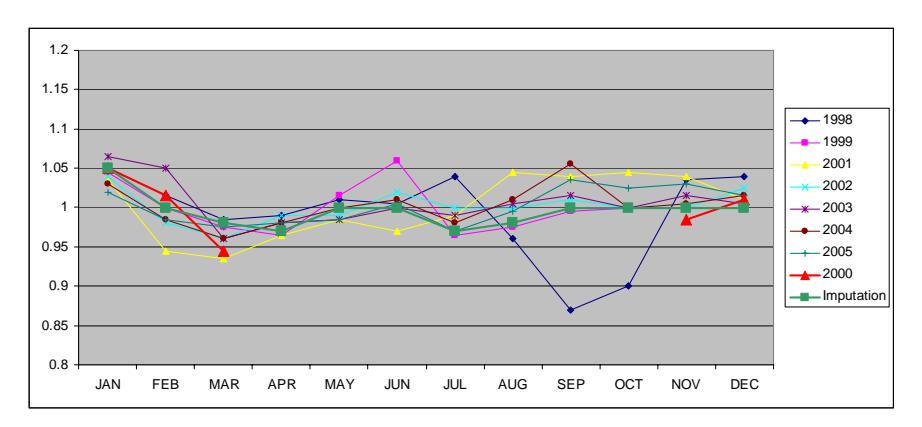
# **B.25 Imputation for Site 799925**
For site 799925, MSFs for all months except November and December are borrowed from 1999. For November and December, MSFs are from 2000.
| | JAN | FEB | MAR APR | | MAY JUN | | JUL | AUG | SEP | OCT | NOV | DEC |
|------------|-------|------|---------|------|---------|-------|-------|-------|-------|-------|-------|-------|
| 1998 | 1.015 | 0.97 | 0.99 | 0.97 | 1.04 | 1.02 | 1.03 | 1.025 | 1.015 | 0.99 | 0.985 | 0.92 |
| 1999 | 1.01 | 0.96 | 0.97 | 1 | 1.02 | 1.03 | 1 | 1.025 | 1.01 | 0.98 | 0.995 | |
| 2001 | 1.01 | | 0.96 | 1 | 1.16 | | | | 1.015 | 1.01 | | |
| 2002 | | 0.97 | 0.945 | 1 | 1.025 | 1.035 | 1.045 | 1.015 | 1.005 | 1.015 | 1.005 | 1.005 |
| 2003 | 0.985 | 0.98 | 0.955 | 1.01 | 1.03 | 1.045 | 1.03 | 1.03 | 1.025 | 0.99 | 0.98 | 0.96 |
| 2004 | 0.99 | 0.97 | 0.96 | 1 | 1.015 | 1.035 | 1.03 | 1.035 | 1.03 | 0.99 | 1.005 | 0.965 |
| 2005 | 0.98 | 0.95 | 0.95 | 0.97 | 1 | 1.02 | 1.015 | 1.03 | 1.025 | 1.02 | 1.02 | 0.985 |
| | | | | | | | | | | | | |
| 2000 | | | | | | | | | | | 1.025 | 0.975 |
| Imputation | 1.01 | 0.96 | 0.97 | 1 | 1.02 | 1.03 | 1 | 1.03 | 1.01 | 0.98 | 1.03 | 0.98 |
| Source | 1999 | 1999 | 1999 | 1999 | 1999 | 1999 | 1999 | 1999 | 1999 | 1999 | 2000 | 2000 |
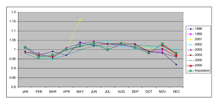
# **B.26 Imputation for Site 890289**
For site 890289, MSFs for all months are borrowed from 2001.
| | JAN | FEB | MAR APR | | MAY JUN | | JUL | AUG | SEP | OCT | NOV | DEC |
|------------|-------|-------|---------|-------|---------|-------|-------|-------|-------|-------|-------|-------|
| 1998 | 0.885 | 0.875 | 0.88 | 0.955 | 1.035 | 1.135 | | 1.12 | 1.115 | 1.065 | 0.985 | 0.94 |
| 1999 | 0.92 | 0.845 | 0.86 | 0.95 | 1.04 | 1.155 | 1.175 | 1.12 | 1.09 | 0.97 | | 0.89 |
| 2001 | 0.92 | 0.87 | 0.86 | 0.945 | 1.065 | 1.12 | 1.16 | 1.115 | 1.12 | 1.06 | 0.96 | 0.915 |
| 2002 | 0.92 | 0.855 | 0.855 | 0.94 | 1.035 | 1.125 | 1.175 | 1.14 | 1.085 | 1.04 | 0.97 | 0.93 |
| 2003 | 0.93 | 0.91 | 0.9 | 0.95 | 1.055 | 1.13 | 1.14 | 1.09 | 1.08 | 1.02 | 0.935 | 0.89 |
| 2004 | 0.97 | | 0.905 | 0.955 | 1.025 | 1.115 | 1.145 | 1.125 | 1.055 | 0.935 | 0.91 | 0.88 |
| 2005 | 0.935 | 0.9 | 0.92 | 0.94 | 1.02 | 1.1 | 1.06 | 1.07 | 1.115 | 1.2 | | 1.05 |
| | | | | | | | | | | | | |
| 2000 | 0.985 | | 0.915 | 1.025 | 1.13 | 1.19 | | | | 0.995 | 0.96 | 0.9 |
| Imputation | 0.92 | 0.87 | 0.86 | 0.95 | 1.07 | 1.12 | 1.16 | 1.12 | 1.12 | 1.06 | 0.96 | 0.92 |
| Source | 2001 | 2001 | 2001 | 2001 | 2001 | 2001 | 2001 | 2001 | 2001 | 2001 | 2001 | 2001 |
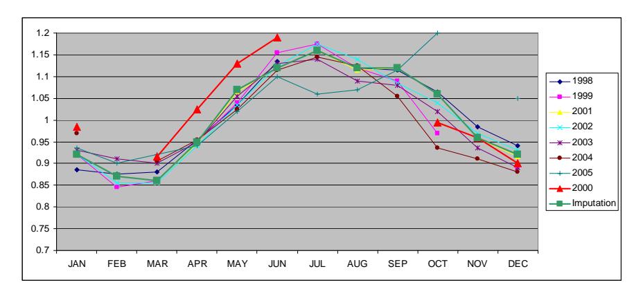
# **B.27 Imputation for Site 920065**
For site 920065, MSFs for all months except October, November, and December are from 2000. For the last three months, MSFs are estimated as the average of year 1998 to 1999, and 2001 to 2005.
| | JAN | FEB | MAR APR | | MAY JUN | | JUL | AUG | SEP | OCT | NOV | DEC |
|------------|-------|-------|---------|-------|---------|-------|-------|-------|-------|----------|-------|-------|
| 1998 | 0.97 | 0.935 | 0.88 | 0.97 | 0.98 | 0.97 | 1.04 | 1.015 | 1.08 | 1.01 | 1.05 | 1.05 |
| 1999 | 1.04 | 0.97 | 0.945 | 0.935 | 1.01 | 0.92 | 0.94 | 1.08 | 1.085 | 1.055 | 1.07 | 1.05 |
| 2001 | 1.07 | 0.96 | 0.95 | 0.94 | 0.99 | 0.98 | 0.985 | 1 | 1.075 | 1.085 | 1.035 | 1.05 |
| 2002 | 1.01 | 0.95 | 0.885 | 0.955 | 1.015 | 1.03 | 1.005 | 1.03 | 1.09 | 1.035 | 1.01 | 1.03 |
| 2003 | 1.025 | 0.97 | 0.91 | 0.975 | 1.01 | 1.015 | 0.975 | 1.025 | 1.09 | 1.015 | 1.025 | 1.005 |
| 2004 | 1.04 | 0.97 | 0.91 | 0.97 | 1.015 | 1.015 | 0.985 | 1.035 | 1.115 | 1.02 | 1.015 | 0.995 |
| 2005 | 1.01 | 0.95 | 0.935 | 0.97 | 1.005 | 1.01 | 0.975 | 1.015 | 1.08 | 1.05 | 1.025 | 0.975 |
| | | | | | | | | | | | | |
| 2000 | 1 | 0.95 | 0.91 | 0.96 | 1.02 | 1.025 | 1.015 | 1.055 | 1.085 | | | |
| Imputation | 1 | 0.95 | 0.91 | 0.96 | 1.02 | 1.03 | 1.02 | 1.06 | 1.09 | 1.04 | 1.03 | 1.02 |
| Source | 2000 | 2000 | 2000 | 2000 | 2000 | 2000 | 2000 | 2000 | | 2000 AVG | AVG | AVG |
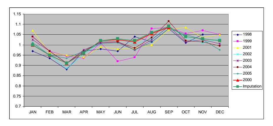
# **B.28 Imputation for Site 939935**
For site 939935, MSFs for all months except January are from 2000. For January, MSF is borrowed from 2001.
| | JAN | FEB | MAR APR | | MAY JUN | | JUL | AUG | SEP | OCT | NOV | DEC |
|------------|-------|-------|---------|-------|---------|-------|-------|-------|-------|-------|-------|-------|
| 1998 | | 0.86 | 0.905 | 1.015 | 1.055 | 1.11 | 1.02 | 1.03 | 1.165 | 1.095 | 0.98 | 0.93 |
| 1999 | | 0.785 | 0.81 | 0.94 | 1.005 | 1.065 | 1.035 | 1.08 | 1.09 | 0.99 | 0.905 | |
| 2001 | 0.935 | 0.9 | 0.925 | 0.97 | 1.035 | 1.05 | 1.06 | 1.07 | 1.14 | 1.06 | 0.94 | 0.79 |
| 2002 | 0.91 | 0.91 | | 0.97 | 0.995 | 1.055 | 1.06 | 1 | 1.09 | 1.015 | 0.925 | 0.925 |
| 2003 | | 0.87 | 0.87 | | | 1.06 | 1.05 | 1.065 | 1.08 | 1.025 | 0.945 | 0.925 |
| 2004 | 0.96 | 0.92 | 0.91 | 0.99 | 1.015 | 1.055 | 1.07 | 1.085 | 1.14 | 1.05 | 0.955 | 0.95 |
| 2005 | 0.975 | 0.92 | 0.915 | 0.975 | 1.02 | 1.075 | 1.06 | 1.11 | 1.11 | 1.105 | 0.945 | 0.88 |
| | | | | | | | | | | | | |
| 2000 | | 0.905 | 0.92 | 0.99 | 1.02 | 1.055 | 1.045 | 1.08 | 1.11 | 1.04 | 0.94 | 0.905 |
| Imputation | 0.94 | 0.91 | 0.92 | 0.99 | 1.02 | 1.06 | 1.05 | 1.08 | 1.11 | 1.04 | 0.94 | 0.91 |
| Source | 2001 | 2000 | 2000 | 2000 | 2000 | 2000 | 2000 | 2000 | 2000 | 2000 | 2000 | 2000 |
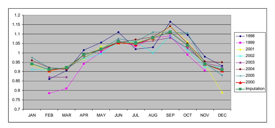
# **APPENDIX C. EMPLOYMENT VARIABLES**
Table gives the name, definition, and a description of each of the employment categories in columns 2, 3, and 4. The first column provides the correspondence SIC code.
| SIC | Variable | Definition | Description |
|-----|----------|---------------------------------------------------------------|--------------------------------------------------------------------------------|
| 1 | AgriP | Agricultural Production-Crops | Agriculture workers as a
percentage of total workers |
| 9 | FishP | Fishing & Hunting workers as a percentage of
total workers | Fishing, hunting, trapping |
| 42 | | Motor Freight Transportation/Warehouse | |
| 43 | TranP | United States Postal Service | Transportation workers as a |
| 44 | | Water Transportation | percentage of total workers |
| 45 | | Transportation by Air | |
| 50 | WholP | Wholesale Trade-Durable Goods | Wholesale workers as a |
| 51 | | Wholesale Trade-Nondurable Goods | percentage of total workers |
| 52 | | Building Materials & Hardware | |
| 53 | | General Merchandise Stores | |
| 54 | | Food Stores | |
| 55 | RetailP | Automotive Dealers & Service Station | Retail workers as a |
| 56 | | Apparel & Accessory Stores | percentage of total workers |
| 57 | | Home Furniture & Furnishings Stores | |
| 59 | | Miscellaneous Retail | |
| 58 | RestaP | Eating & Drinking Places | Restaurant workers as a
percentage of total workers |
| 70 | HotelP | Hotels Rooming Houses & Camps | Hotel & Camp workers as a
percentage of total workers |
| 82 | EduP | Educational Services | Education workers as a
percentage of total workers |
| 79 | | RecServP Amusement & Recreation Services | Amusement & Recreation
Services workers as a
percentage of total workers |
| 84 | | MuseumP Museums Art Galleries & Gardens | Museums Art Galleries &
Gardens workers as a
percentage of total workers |
| 10 | | Metal Mining | |
| 12 | | Coal Mining | Mining workers as a |
| 13 | MineP | Oil & Gas Extraction | percentage of total workers |
| 14 | | Mining & Quarrying-Nonmetallic Miner | |
| 20 | ManuP | Food & Kindred Products Manufacture | Manufacturing workers as a |
| 21 | | Tobacco Products Manufacturing | percentage of total workers |
| 22 | | Textile Mill Products Manufacturing | |
| 23 | | Apparel & Other Finished Products
Manufacturing | |
| 24 | | Lumber & Wood Prods Except Furniture
Manufacturing | |
| 25 | | Furniture & Fixtures Manufacturing | |
| 26 | | Paper & Allied Products Manufacturing | |
| 27 | | Printing Publishing & Allied Industry | |
| | | | |
| 28 | | Chemicals & Allied Products Manufacturing | |
|----|-------|--------------------------------------------|-------------------------------|
| | | Petroleum Refining & Related Industry | |
| 29 | | Manufacturing | |
| | | Rubber & Miscellaneous Plastics | |
| 30 | | Manufacturing | |
| 31 | | Leather & Leather Products Manufacturing | |
| 32 | | Stone Clay Glass & Concrete Products | |
| | | Manufacturing | |
| 33 | | Primary Metal Industries Manufacturing | |
| 34 | | Fabricated Metal Products Manufacturing | |
| 35 | | Industrial & Commercial Machinery | |
| | | Manufacturing | |
| 36 | | Electronic & Other Electrical Equipment | |
| 37 | | Transportation Equipment Manufacturing | |
| 38 | | Measuring & Analyzing Instruments | |
| | | Manufacturing | |
| 39 | | Miscellaneous Industries Manufacturing | |
| 60 | | Depository Institutions | |
| 61 | | Non-depository Credit Institutions | |
| 62 | | Security & Commodity Brokers | |
| 63 | | Insurance Carriers | |
| 64 | | Insurance Agents Brokers & Service | |
| 65 | | Real Estate | |
| 67 | | Holding & Other Investment Offices | Service workers as a |
| 72 | ServP | Personal Services | percentage of total workers |
| 73 | | Business Services | |
| 75 | | Auto Repair Services & Parking | |
| 81 | | Legal Services | |
| 83 | | Social Services | |
| 87 | | Engineering & Accounting & management | |
| | | Services | |
| 86 | | Membership Organizations | |
| 91 | | Executive Legislative & General Government | |
| 92 | | Justice Public Order & Safety | |
| 93 | | Public Finance & Taxation Policy | |
| 94 | | Administration-Human Resource | Office workers s a percentage |
| | ServP | Programs | of total workers |
| 95 | | Admin-Environmental Quality Programs | |
| 96 | | Administration of Economic Programs | |
| 97 | | National Security & International | |
| | | Affair | |
#### **APPENDIX D. LIST OF MODEL VARIABLES**
#### **Variables for Urban Area and Rural Area**
| ia
V
b
le
ar | ip
io
D
t
es
cr
n | R
an
g
e | So
ur
ce | U
da
te
p
Fr
eq
ue
nc
y |
|----------------------------|--------------------------------------------------------------------------------------------------------------------------------------------------------------------------------------------------------------------------|--------------------------------------------------------|---------------------------------|-------------------------------------------------|
| R
Lo
t_
w | Pe
f r
ire
d
H
H
i
h
lo
in
f
l
ho
ho
l
ds
ta
t
t
t o
to
ta
rc
en
g
e
o
e
s w
co
m
e
ou
us
e
w | 0-
4
8.
9
6
1
8 | C
en
su
s | 1
0
ea
rs
y |
| h
R
H
ig
t_ | Pe
f r
ire
d
H
H
i
h
h
ig
h
in
f
l
ho
ho
l
ds
ta
t
t
t o
to
ta
rc
en
g
e
o
e
s w
co
m
e
ou
us
e | 0-
3
8.
7
5
8
9 | C
en
su
s | 1
0
ea
rs
y |
| R
E
T
I
R
E | Pe
f r
ire
d
H
H
f
l
ho
ho
l
ds
ta
t
t o
to
ta
rc
en
g
e
o
e
s o
u
us
e | 1.
5
6
7
2-
6
5.
7
6
2
9 | C
en
su
s | 1
0
y
ea
rs |
| A
i
P
g
r | A
ic
l
ke
f
l w
ke
tu
ta
to
ta
g
r
u
re
w
or
rs
a
s a
p
er
ce
n
g
e
o
or
rs | 0-
5
6.
7
0
7
1 | I
N
F
O
U
S
A | ev
er
y
y
ea
r |
| F
is
h
P | is
h
in
in
ke
f
l w
ke
F
&
H
t
ta
to
ta
g
un
g
w
or
rs
a
s a
p
er
ce
n
g
e
o
or
rs | 0-
2.
2
5 | I
N
F
O
U
S
A | ev
er
y
y
ea
r |
| Tr
P
an | io
ke
f
l w
ke
Tr
ta
t
ta
to
ta
an
sp
or
n
w
or
rs
a
s a
p
er
ce
n
g
e
o
or
rs | 0-
5
2.
1
2
5
5 | I
N
F
O
U
S
A | ev
er
y
y
ea
r |
| ho
l
W
P | ho
le
le
ke
f
l w
ke
W
ta
to
ta
sa
w
or
rs
a
s a
p
er
ce
n
g
e
o
or
rs | 0-
7
3.
2
5
4
6 | O
S
A
I
N
F
U | ev
er
y
y
ea
r |
| Re
P
t
s | ke
f
l w
ke
R
ta
t w
ta
to
ta
es
er
ce
e
ur
an
or
rs
a
s a
p
n
g
o
or
rs | 0-
9.
1
5
5
7
7 | O
S
A
I
N
F
U | ev
er
ea
y
y
r |
| d
E
P | du
io
ke
f
l w
ke
E
t
ta
to
ta
ca
n
or
rs
a
s a
p
er
ce
n
g
e
o
or
rs
w | 0-
6.
0
1
8
0
7 | O
S
A
I
N
F
U | ev
er
ea
r
y
y |
| Se
Re
P
c
rv | A
&
R
io
Se
ic
ke
t
t
ta
m
us
em
en
ec
re
a
n
rv
es
or
rs
a
s a
p
er
ce
n
g
e
w
f
l w
ke
to
ta
o
or
rs | 0-
5
3.
9
7
3
5 | I
N
F
O
U
S
A | ev
er
ea
r
y
y |
| M
in
P
e | M
in
in
ke
f
l w
ke
ta
to
ta
g
w
or
rs
a
s a
p
er
ce
n
g
e
o
or
rs | 0-
4
7.
5 | I
N
F
O
U
S
A | ev
er
y
y
ea
r |
| M
P
an
u | M
fa
in
ke
f
l w
ke
tu
ta
to
ta
an
u
c
r
g
w
or
rs
a
s a
p
er
ce
n
g
e
o
or
rs | 0-
9
5.
7 | I
N
F
O
U
S
A | ev
er
y
y
ea
r |
| Se
P
rv | Se
ic
ke
f
l w
ke
ta
to
ta
rv
es
w
or
rs
a
s a
p
er
ce
n
g
e
o
or
rs | 0-
1
0
4 | I
N
F
O
U
S
A | ev
er
y
y
ea
r |
| O
f
f
P | f
f
ic
ke
f
l w
ke
O
ta
to
ta
e
w
or
rs
a
s a
p
er
ce
n
g
e
o
or
rs | 0-
2
3.
6
7 | I
N
F
O
U
S
A | ev
er
y
y
ea
r |
| S
T
1 | la
io
de
l
d
Po
4
t
ta
p
u
n
p
er
ce
n
g
e u
n
r
y
ea
rs
o | 0.
0
0
0
1-
0.
0
4
9
7 | C
en
su
s | 1
0
y
ea
rs |
| S
T
2 | la
io
f
A
Po
5-
1
7
t
ta
p
u
n
p
er
ce
n
g
e
o
g
e | 0.
0
0
0
5-
0.
2
3
2
7 | C
en
su
s | 1
0
y
ea
rs |
| 2
1
S
T
U | la
io
f
A
1
0
Po
5-
t
ta
er
ce
e
e
p
u
n
p
n
g
o
g | 0.
0
0
0
2-
0.
0
8
4
7 | C
en
su
s | 1
0
ea
y
rs |
| 2
2
S
T
U | la
io
f
A
1
1-
1
3
Po
t
ta
p
n
p
er
ce
n
g
e
o
g
e
u | 0.
0
0
0
1-
0.
0
2
9
5 | C
en
su
s | 1
0
ea
rs
y |
| S
2
3
T
U | Po
la
io
f
A
1
4-
1
7
t
ta
p
n
p
er
ce
n
g
e
o
g
e
u | 0.
0
0
0
1-
0.
0
9
2
5 | C
en
su
s | 1
0
ea
rs
y |
| M
In
c | M
d
ia
ho
ho
l
d
in
e
n
us
e
co
m
e | 1
9
2
3
5-
7
0
9
3
9 | C
en
su
s | 1
0
y
ea
rs |
# **Variables for Urban Area Only**
| V
ia
b
le
ar | D
ip
io
t
es
cr
n | R
an
g
e | So
ur
ce | U
da
te
p
Fr
eq
ue
nc
y |
|--------------------------|----------------------------------------------------------------------------------------------------------------------------------------------------------------------------------|-------------------|----------------|-------------------------------------------------|
| F
R | ls
1
i
f
S
is
lo
d
ba
fr
0
he
is
Eq
T
T
M
te
t
ua
ca
on
a
u
r
n
ee
w
ay
;
o
rw
e | 0
1
or | F
T
I | ev
er
y
y
ea
r |
| ia
V
b
le
ar | ip
io
D
t
es
cr
n | R
an
g
e | So
ur
ce | U
da
te
p
Fr
eq
ue
nc
y |
|--------------------------|------------------------------------------------------------------------------------------------------------------------------------------------------------------------------------------------------------------------------------------------------------------------------------------------------------------------------------|--------------------------------------------------------|---------------------------------|-------------------------------------------------|
| A
P | Eq
ls
1
i
f
T
T
M
S
is
lo
d
ba
in
ip
le
ia
l;
0
te
te
ua
ca
on
a
r
n
p
r
c
a
r
r
u
he
is
t
o
rw
e | 0
1
or | F
T
I | ev
er
ea
r
y
y |
| M
A | Eq
ls
1
i
f
T
T
M
S
is
lo
d
ba
in
ia
l;
0
te
te
ua
ca
on
a
r
n
m
or
a
r
r
u
he
is
t
o
rw
e | 0
1
or | F
T
I | ev
er
ea
r
y
y |
| C
O | Eq
ls
1
i
f
T
T
M
S
is
lo
d
ba
l
le
0
he
is
te
to
t
ua
ca
on
a
r
n
co
c
r;
o
rw
e
u | 0
1
or | F
T
I | ev
er
ea
r
y
y |
| G
L
E | Eq
ls
1
i
f
T
T
M
S
is
lo
d
in
Le
C
0
he
is
te
ty
t
ua
ca
on
ou
n
;
o
rw
e | 0
1
or | | N
/
A |
| S
U | Eq
ls
1
i
f
T
T
M
S
is
in
he
f
U
F,
F
S
U
d
F
A
M
U
i
h
in
t
ty
t
ua
c
ou
n
o
an
;
or
w
,
hr
i
le
f
U
M
F
I
T;
0
he
is
t
t
ee
m
s o
o
r
o
rw
e | 0
1
or | | N
/
A |
| F
U | Eq
ls
1
i
f
T
T
M
S
is
lo
d
i
h
in
hr
i
le
f o
he
iv
i
ie
te
t
t
t
ta
te
t
ua
ca
w
ee
m
s o
r s
u
n
er
s
s;
0
he
is
t
o
rw
e | 0
1
or | | N
/
A |
| D
I
S
N | ls
i
f
is
lo
d
in
la
he
is
Eq
1
T
T
M
S
O
C
0
te
ty
t
ua
ca
sc
eo
ou
n
;
o
rw
e | 0
1
or | | /
N
A |
| L
U
1 | ls
i
f
bu
f
fe
is
in
im
in
be
h
la
d
Eq
1
T
T
M
S
0
ua
r
co
ve
r
g
sw
m
g
ac
n
us
e
ar
ea
;
he
is
t
o
rw
e | 0
1
or | F
G
D
L | /
N
A |
| L
U
2 | ls
i
f
bu
f
fe
is
in
l
f c
la
d
he
is
Eq
1
T
T
M
S
0
t
ua
r
co
ve
r
g
g
o
ou
rs
e
n
us
e
ar
ea
;
o
rw
e | 0
1
or | F
G
D
L | /
N
A |
| L
U
3 | ls
i
f
S
bu
f
fe
is
in
in
d
f
is
h
la
d
Eq
1
T
T
M
ua
r
co
ve
r
g
m
ar
as
a
n
ca
m
p
s
n
us
e
ar
ea
;
he
is
0
t
o
rw
e | 0
1
or | F
G
D
L | /
N
A |
| L
U
4 | ls
1
i
f
S
bu
f
fe
is
in
ks
d
la
d
0
Eq
T
T
M
ua
r
co
ve
r
g
p
ar
a
n
zo
os
n
us
e
ar
ea
;
he
is
t
o
rw
e | 0
1
or | G
F
D
L | /
A
N |
| S
H
P | f
Se
l
ho
ho
l
ds
Pe
ta
rc
en
g
e
o
as
on
a
us
e | 0-
8
9.
1
9
2
7 | C
en
su
s | 1
0
y
ea
rs |
| l
R
P
t | i
l w
ke
f
l w
ke
R
ta
ta
to
ta
e
or
rs
a
s a
p
er
ce
n
g
e
o
or
rs | 1.
3
9
3-
6
4.
3
4
2
5
7 | O
S
A
I
N
F
U | ev
er
ea
r
y
y |
| l
H
P
t
o | H
l
&
C
ke
f
l w
ke
te
ta
to
ta
o
am
p
or
rs
a
s a
p
er
ce
n
g
e
o
or
rs
w | 0-
2
0.
3
0
1
7 | I
N
F
O
U
S
A | ev
er
ea
r
y
y |
| M
P
se
um | l
ler
ies
de
ke
f
l w
ke
M
&
t g
tag
to
ta
us
eu
m
s a
r
a
g
ar
ns
w
or
rs
as
a
p
er
ce
n
e o
or
rs | 0.
-1
4
3
2
0 | I
N
F
O
U
S
A | ev
er
ea
r
y
y |
# **Variables for Rural Area Only**
| V
ia
b
le
ar | D
ip
io
t
es
cr
n | R
an
g
e | So
ur
ce | U
da
te
p
Fr
eq
ue
nc
y |
|--------------------------|-----------------------------------------------------------------------------------------------------------------------------------------------------------------------------------------------------------------|-------------------|----------------|-------------------------------------------------|
| P
A | ls
i
f
is
lo
d
l p
in
ip
le
ia
l;
Eq
1
T
T
M
S
te
te
ua
ca
on
a
ru
ra
r
c
a
r
r
0
he
is
t
o
rw
e | 0
1
or | F
T
I | ev
er
y
y
ea
r |
| M
A | ls
i
f
is
lo
d
l m
in
ia
l;
Eq
1
T
T
M
S
0
te
te
ua
ca
on
a
ru
ra
or
a
r
r
he
is
t
o
rw
e | 0
1
or | F
T
I | ev
er
y
y
ea
r |
| ia
V
b
le
ar | ip
io
D
t
es
cr
n | R
an
g
e | So
ur
ce | U
da
te
p
Fr
eq
ue
nc
y |
|------------------------------------|-----------------------------------------------------------------------------------------------------------------------------------------------------------------------------------------------------------------------------------------------------------------------------------------------------------------------------------------------------------------------------------|-------------------------------------------------------------|---------------------------------|-------------------------------------------------|
| C
O | Eq
ls
1
i
f
T
T
M
S
is
lo
d
l c
l
le
0
he
is
te
to
t
ua
ca
on
a
ru
ra
o
c
r;
o
rw
e | 0
1
or | F
T
I | ev
er
ea
r
y
y |
| T
F | Tr
k
fa
to
uc
c
r | 1.
6
0-
4
1.
0
8 | F
T
I | ev
er
ea
r
y
y |
| A
5
P
P | Po
la
io
d
5
d
de
f
l p
la
io
t
ta
to
ta
t
p
u
n
ag
e
an
un
r a
s a
p
er
ce
n
g
e
o
op
u
n | 0.
0
2
0
9-
0.
1
4
6
2 | C
en
su
s | 1
0
y
ea
rs |
| P
P
A
6_
1
7 | la
io
d
be
d
l p
la
io
Po
6
1
7
f
t
tw
ta
to
ta
t
p
u
n
ag
e
ee
n
an
as
a
p
er
ce
n
g
e
o
op
u
n | 0.
0
2
6
0-
0.
3
5
0
8 | C
en
su
s | 1
0
y
ea
rs |
| P
P
A
2
2_
6
4 | la
io
d
be
d
f
l p
la
io
Po
2
2
6
4
t
tw
ta
to
ta
t
p
u
n
ag
e
ee
n
an
as
a
p
er
ce
n
g
e
o
op
u
n | 0.
4
0
0
3-
0.
7
9
6
4 | C
en
su
s | 1
0
y
ea
rs |
| P
P
A
1
8_
6
4 | la
io
d
be
d
f
l p
la
io
Po
1
8
6
4
t
tw
ta
to
ta
t
p
u
n
ag
e
ee
n
an
as
a
p
er
ce
n
g
e
o
op
u
n | 0.
4
3
5
6-
0.
8
4
3
9 | C
en
su
s | 1
0
y
ea
rs |
| 6_
P
P
A
2
1 | la
io
d
be
6
d
2
1
f
l p
la
io
Po
t
tw
ta
to
ta
t
p
u
n
ag
e
ee
n
an
as
a
p
er
ce
n
g
e
o
op
u
n | 0.
0
3
9
9-
0.
4
0
2
2 | C
en
su
s | 1
0
y
ea
rs |
| 1
8_
2
1
P
P
A | la
io
d
be
1
8
d
2
1
f
l p
la
io
Po
t
tw
ta
to
ta
t
p
n
ag
e
ee
n
an
as
a
p
er
ce
n
g
e
o
op
n
u
u | 0.
0
1
0
3-
0.
1
1
0
7 | C
en
su
s | 1
0
ea
rs
y |
| 6
P
P
A
5u
p | la
io
d
6
d
f
l p
la
io
Po
5
t
ta
to
ta
t
p
n
ag
e
an
ov
er
a
s a
p
er
ce
n
g
e
o
op
n
u
u | 0.
0
2
6
1-
0.
4
0
8
2 | C
en
su
s | 1
0
ea
rs
y |
| A
5
P
D | Po
la
io
de
i
d
5
d
de
t
ty
p
n
ns
a
g
e
an
un
r
u | 0.
0
0
0
1-
0.
0
6
2
3 | C
en
su
s | 1
0
ea
rs
y |
| A
6_
1
7
P
D | Po
la
io
de
i
d
be
6
d
1
7
t
ty
tw
p
u
n
ns
a
g
e
ee
n
an | 0.
0
0
0
5-
0.
2
2
0
2 | C
en
su
s | 1
0
y
ea
rs |
| P
D
A
2
2_
6
4 | Po
la
io
de
i
d
be
2
2
d
6
4
t
ty
tw
p
u
n
ns
a
g
e
ee
n
an | 0.
0
0
1
5-
0.
5
3
0
3 | C
en
su
s | 1
0
y
ea
rs |
| P
D
A
1
8_
6
4 | la
io
de
i
d
be
d
Po
1
8
6
4
t
ty
tw
p
u
n
ns
a
g
e
ee
n
an | 0.
0
0
1
6-
0.
5
6
6
2 | C
en
su
s | 1
0
y
ea
rs |
| P
D
A
6_
2
1 | la
io
de
i
d
be
d
Po
6
2
1
t
ty
tw
p
u
n
ns
a
g
e
ee
n
an | 0.
0
0
0
5-
0.
2
5
6
1 | C
en
su
s | 1
0
y
ea
rs |
| P
D
A
1
8_
2
1 | la
io
de
i
d
be
d
Po
1
8
2
1
t
ty
tw
p
u
n
ns
a
g
e
ee
n
an | 0.
0
0
0
1-
0.
0
3
5
9 | C
en
su
s | 1
0
y
ea
rs |
| 6
P
D
A
5u
p | la
io
de
i
d
6
d
Po
5
t
ty
p
u
n
ns
a
g
e
an
ov
er | 0.
0
0
0
2-
0.
1
2
8
2 | C
en
su
s | 1
0
y
ea
rs |
| 1
D
is
t | f r
io
f
la
io
f a
l
i
he
d
is
fr
M
Po
t
t
tro
ta
to
t
ta
ax
o
a
o
p
n
o
m
e
p
o
n
ar
ea
nc
e
om
u
he
S
he
l
i
(
/m
i
le
)
T
T
M
M
t
to
t
tro
ta
e
p
o
n
ar
ea
p
er
so
n | 8
2
1
0-
1
1
8
3
6
5 | C
en
su
s | 1
0
ea
rs
y |
| de
d
In
is
2
t
x | l
i
la
io
M
tro
ta
t
e
p
o
n
p
op
u
n
∑
-5
−1 )
(
(
1
0
D
is
fr
he
T
T
M
S
he
l
i
ta
t
to
t
tro
ta
nc
e
om
m
e
p
o
n
ar
ea
i
le
/p
)
m
er
so
n | 0.
9
3-
2.
6
8
3
3
5
5
5
5 | C
en
su
s | 1
0
y
ea
rs |
| In
d
is
te
t
r | is
fr
he
lo
h
ig
hw
in
ha
(
i
le
)
D
T
T
M
S
ta
to
t
t
te
nc
e
om
a
c
se
s
ay
rc
ng
e
m | 4
6
5-
1
1
2
3
8
6 | | |
| h
d
Be
is
t
ac | is
fr
S
he
lo
be
h
i
(
)
D
T
T
M
ta
to
t
t
te
te
nc
e
om
a
c
se
s
ac
s
m
e
r | 0.
6
1-
1
2
0.
6
7 | | |
| N
S
H
P | f s
l
ho
ho
l
ds
in
he
lo
i
da
Pe
F
ta
t
rc
en
g
e
o
ea
so
na
us
e
n
or
rn
r | 0-
9
6.
4
3
2
1 | C
en
su
s | 1
0
ea
rs
y |
| C
S
H
P | Pe
f s
l
ho
ho
l
ds
in
l
F
lo
i
da
ta
tra
rc
en
g
e
o
ea
so
na
us
e
c
en
r | 0-
2
4.
6
4
0
6 | C
en
su
s | 1
0
ea
rs
y |
| S
S
H
P | Pe
f s
l
ho
ho
l
ds
in
he
F
lo
i
da
ta
t
rc
en
g
e
o
ea
so
na
us
e
s
ou
rn
r | 0-
9
2.
8
2
5
3 | C
en
su
s | 1
0
y
ea
rs |
| N
H
l
P
t
o | H
l
&
C
ke
f
l w
ke
in
he
te
ta
to
ta
t
o
am
p
w
or
rs
a
s a
p
er
ce
n
g
e
o
or
rs
n
or
rn
F
lo
i
da
r | 0-
4
2.
6
9
6
6 | I
N
F
O
U
S
A | ev
er
y
y
ea
r |
| C
H
l
P
t
o | l
ke
f
l w
ke
in
l
H
&
C
te
ta
to
ta
tra
o
am
p
w
or
rs
a
s a
p
er
ce
n
g
e
o
or
rs
c
en
F
lo
i
da
r | 0-
6.
6
4
7
3 | I
N
F
O
U
S
A | ev
er
y
y
ea
r |
| V
ia
b
le
ar | D
ip
io
t
es
cr
n | R
an
g
e | So
ur
ce | U
da
te
p
Fr
eq
ue
nc
y |
|----------------------------|-------------------------------------------------------------------------------------------------------------------------------------------------------------------------------------------------------------------------------------------------------------------------------------------|-----------------------------------|---------------------------------|-------------------------------------------------|
| S
H
l
P
t
o | l
ke
f
l w
ke
in
he
H
&
C
te
ta
to
ta
t
o
am
p
w
or
rs
a
s a
p
er
ce
n
g
e
o
or
rs
s
ou
rn
lo
i
da
F
r | 0-
1
3.
0
3
5
7 | I
N
F
O
U
S
A | ev
er
y
y
ea
r |
| N
R
l
P
t | i
l w
ke
f
l w
ke
in
he
lo
i
da
R
F
ta
ta
to
ta
t
e
or
rs
a
s a
p
er
ce
n
g
e
o
or
rs
n
or
rn
r | 0-
7
1.
2
2
7
3 | I
N
F
O
U
S
A | ev
er
y
y
ea
r |
| C
R
l
P
t | i
l w
ke
f
l w
ke
in
l
lo
i
da
R
F
ta
ta
to
ta
tra
e
or
rs
a
s a
p
er
ce
n
g
e
o
or
rs
c
en
r | 0-
2
1.
1
5
6
3 | I
N
F
O
U
S
A | ev
er
y
y
ea
r |
| l
S
R
P
t | i
l w
ke
f
l w
ke
in
he
lo
i
da
R
F
ta
ta
to
ta
t
e
or
rs
a
s a
p
er
ce
n
g
e
o
or
rs
s
ou
rn
r | 0-
1
9.
0
1
5
7 | O
S
A
I
N
F
U | ev
er
y
y
ea
r |
| N
M
P
se
m | l
le
ie
&
de
ke
f
l
M
t g
ta
to
ta
eu
er
ce
e
us
m
s a
r
a
r
s
g
ar
ns
w
or
rs
a
s a
p
n
g
o
ke
in
he
lo
i
da
F
t
w
or
rs
n
or
rn
r | 0-
0.
6
9
8
6 | O
S
A
I
N
F
U | ev
er
y
y
ea
r |
| C
M
P
se
m | l
le
ie
&
de
ke
f
l
M
t g
ta
to
ta
us
eu
m
s a
r
a
r
s
g
ar
ns
or
rs
a
s a
p
er
ce
n
g
e
o
w
ke
in
l
lo
i
da
F
tra
en
w
or
rs
c
r | 0-
0.
2
4
6
2 | O
S
A
I
N
F
U | ev
er
ea
r
y
y |
| S
M
P
se
m | M
l
le
ie
&
de
ke
f
l
t g
ta
to
ta
us
eu
m
s a
r
a
r
s
g
ar
ns
or
rs
a
s a
p
er
ce
n
g
e
o
w
ke
in
he
lo
i
da
F
t
or
rs
s
ou
rn
r
w | 0-
1.
2
5 | O
S
A
I
N
F
U | ev
er
ea
r
y
y |