category: literaturenote citekey: ehsanisustainabletransportation2013 title: Sustainable Transportation authors: "Ehsani, Mehrdad" year: 2013 date: 2013-00-00 2013 doi: 10.1007/978-1-4614-5844-9_795 url: "https://doi.org/10.1007/978-1-4614-5844-9_795" zotero_key: EMGCIWHJ zotero_storage: FJ34M28J collections: transpordi_planeerimine folder: 001_artiklid firstAuthor: "Ehsani, Mehrdad"

status: converted

Transportation Technologies for Sustainability

This volume collects selected topical entries from the Encyclopedia of Sustainability Science and Technology (ESST). ESST addresses the grand challenges for science and engineering today. It provides unprecedented, peer-reviewed coverage of sustainability science and technology with contributions from nearly 1,000 of the world's leading scientists and engineers, who write on more than 600 separate topics in 38 sections. ESST establishes a foundation for the research, engineering, and economics supporting the many sustainability and policy evaluations being performed in institutions worldwide.

Editor-in-Chief

ROBERT A. MEYERS, RAMTECH LIMITED, Larkspur, CA, USA

Editorial Board

RITA R. COLWELL, Distinguished University Professor, Center for Bioinformatics and Computational Biology, University of Maryland, College Park, MD, USA

ANDREAS FISCHLIN, Terrestrial Systems Ecology, ETH-Zentrum, Zu¨rich, Switzerland DONALD A. GLASER, Glaser Lab, University of California, Berkeley, Department of Molecular & Cell Biology, Berkeley, CA, USA

TIMOTHY L. KILLEEN, National Science Foundation, Arlington, VA, USA

HAROLD W. KROTO, Francis Eppes Professor of Chemistry, Department of Chemistry and Biochemistry, The Florida State University, Tallahassee, FL, USA

AMORY B. LOVINS, Chairman & Chief Scientist, Rocky Mountain Institute, Snowmass, USA LORD ROBERT MAY, Department of Zoology, University of Oxford, Oxford, OX1 3PS, UK DANIEL L. MCFADDEN, Director of Econometrics Laboratory, University of California, Berkeley, CA, USA THOMAS C. SCHELLING, 3105 Tydings Hall, Department of Economics, University of Maryland, College Park, MD, USA

CHARLES H. TOWNES, 557 Birge, University of California, Berkeley, CA, USA

EMILIO AMBASZ, Emilio Ambasz & Associates, Inc., New York, NY, USA

CLARE BRADSHAW, Department of Systems Ecology, Stockholm University, Stockholm, Sweden TERRY COFFELT, Research Geneticist, Arid Land Agricultural Research Center, Maricopa, AZ, USA MEHRDAD EHSANI, Department of Electrical & Computer Engineering, Texas A&M University, College Station, TX, USA

ALI EMADI, Electrical and Computer Engineering Department, Illinois Institute of Technology, Chicago, IL, USA

CHARLES A. S. HALL, College of Environmental Science & Forestry, State University of New York, Syracuse, NY, USA

RIK LEEMANS, Environmental Systems Analysis Group, Wageningen University, Wageningen, The Netherlands

KEITH LOVEGROVE, Department of Engineering (Bldg 32), The Australian National University, Canberra, Australia

TIMOTHY D. SEARCHINGER, Woodrow Wilson School, Princeton University, Princeton, NJ, USA

Transportation Technologies for Sustainability

With 826 Figures and 172 Tables

Editors Mehrdad Ehsani Department of Electrical & Computer Engineering Texas A&M University College Station, TX, USA

Fei-Yue Wang Institute of Automation Chinese Academy of Sciences Beijing, China

Gary L. Brosch Center for Urban Transportation Research University of South Florida Tampa, FL, USA

ISBN 978-1-4614-5843-2 ISBN 978-1-4614-5844-9 (eBook) ISBN 978-1-4614-5845-6 (print and electronic bundle) DOI 10.1007/978-1-4614-5844-9 Springer New York Dordrecht Heidelberg London

Library of Congress Control Number: 2012953371

© Springer Science+Business Media New York 2013

This work is subject to copyright. All rights are reserved by the Publisher, whether the whole or part of the material is concerned, specifically the rights of translation, reprinting, reuse of illustrations, recitation, broadcasting, reproduction on microfilms or in any other physical way, and transmission or information storage and retrieval, electronic adaptation, computer software, or by similar or dissimilar methodology now known or hereafter developed. Exempted from this legal reservation are brief excerpts in connection with reviews or scholarly analysis or material supplied specifically for the purpose of being entered and executed on a computer system, for exclusive use by the purchaser of the work. Duplication of this publication or parts thereof is permitted only under the provisions of the Copyright Law of the Publisher's location, in its current version, and permission for use must always be obtained from Springer. Permissions for use may be obtained through RightsLink at the Copyright Clearance Center. Violations are liable to prosecution under the respective Copyright Law.

The use of general descriptive names, registered names, trademarks, service marks, etc. in this publication does not imply, even in the absence of a specific statement, that such names are exempt from the relevant protective laws and regulations and therefore free for general use.

While the advice and information in this book are believed to be true and accurate at the date of publication, neither the authors nor the editors nor the publisher can accept any legal responsibility for any errors or omissions that may be made. The publisher makes no warranty, express or implied, with respect to the material contained herein.

This book consists of selection from the Encyclopedia of Sustainability Science and Technology edited by Robert A. Meyers, published by Springer New York in 2012.

Printed on acid-free paper

Springer is part of Springer Science+Business Media (www.springer.com)

Editors

Electric, Hybrid, and Fuel Cell Vehicles

MEHRDAD EHSANI (also one of the board members) Department of Electrical & Computer Engineering Texas A&M University College Station, TX USA

Mass Transit Science and Technology

GARY L. BROSCH Center for Urban Transportation Research University of South Florida Tampa, FL USA

Intelligent Vehicles Technology

FEI-YUE WANG Institute of Automation Chinese Academy of Sciences Beijing China

Sections

Electric, Hybrid and Fuel Cell Vehicles Editor: Mehrdad Ehsani

AC Machines: Permanent Magnet Synchronous and Induction Machines

Batteries, Battery Management, and Battery Charging Technology

Battery Technologies

Electric, Hybrid, and Fuel Cell Vehicles, Introduction

Electric, Hybrid Electric and Fuel Cell Vehicles, Architectures of

Energy Storage: Ultracapacitor

Fuel-Cell-Powered HEV Design and Control

Hybrid Electric and Hydraulic Technology Applications in Off-Road Vehicles

Hybrid Energy Storage Systems for Vehicle Applications

Internal Combustion Engines, Alternative Fuels for

PHEVs and BEVs in Coupled Power and Transportation Systems

Plug-in Hybrid Electric Vehicles

Regenerative Braking

Sustainable Transportation

Sustainable Vehicle Fuels, Well-to-Wheel Analysis

Switched Reluctance Motor Drives for Propulsion and Regenerative Braking in EV and HEV

Vehicle Biofuels

Vehicle Dynamics and Performance

Vehicle Energy Storage: Batteries

Vehicle Traction Motors

Intelligent Vehicle Technology Editor: Fei-Yue Wang

3D Pose Estimation of Vehicles Using Stereo Camera

Active Multifocal Vision System, Adaptive Control of

Active Pedestrian Protection System, Scenario-Driven Search Method for

Cooperative Group of Vehicles and Dangerous Situations, Recognition of

Driver Assistance System, Biologically Inspired

Driver Assistance Systems, Automatic Detection and Site Mapping

Driver Behavior at Intersections

Driver Characteristics Based on Driver Behavior

Driver Inattention Monitoring System for Intelligent Vehicles

Driving Under Reduced Visibility Conditions for Older Adults

Dynamic Environment Sensing Using an Intelligent Vehicle

Intelligent Vehicles Technology, Introduction

Night Vision Pedestrian Warning in Intelligent Vehicles

True Color Night Vision Video Systems in Intelligent Vehicles

Unscented Kalman Filter in Intelligent Vehicles Vehicle Detection, Tightly Coupled LIDAR and Computer Vision Integration for Vehicular Ad Hoc Networks, Enhanced GPSR and Beacon-Assist Geographic Forwarding in

Mass Transit Science and Technology Editor: Gary L. Brosch

Advanced Public Transport Systems, Simulation-Based Evaluation

Bicycle Integration with Public Transport

Bus Rapid Transit and Light Rail Transit Systems: State of Discussion

Bus Rapid Transit, Institutional Issues Related to Implementation

Bus Rapid Transit: Worldwide History of Development, Key Systems and Policy Issues

Bus Rapid Versus Light Rail Transit: Service Quality, Economic, Environmental, and Planning Aspects

Bus Versus Rail Implications for Transit-Oriented Development

High Speed Rail, Technology Development of

High-Occupancy Vehicle and Toll Lanes

HOT Lanes/Value Pricing: Planning and Evaluation of Multiclass Service

Light Rail Transit in the US and Abroad, Examination of History and Innovations

Light Rail Transit, Shared Infrastructural Issues

Light Rail Transit, Systemic Viability

MAGLEV Technology Development

Mass Transit Science and Technology, Introduction

Personal Rapid Transit and Its Development

Transit-Oriented Development and Land Use

3D Pose Estimation of Vehicles Using Stereo Camera Bjo¨rn Barrois, Christian Wo¨hler	1
AC Machines: Permanent Magnet Synchronous and Induction Machines10.1007/978-1-4419-0851-3_870
A. H. Ranjbar, Babak Fahimi	25
Active Multifocal Vision System, Adaptive Control of10.1007/978-1-4419-0851-3_472
Alois Unterholzner, Hans-Joachim Wuensche	55
Active Pedestrian Protection System, Scenario-Driven Search Method for10.1007/978-1-4419-0851-3_486 Alberto Broggi, Pietro Cerri, Stefano Ghidoni, Paolo Grisleri, Ho Gi Jung	74
Advanced Public Transport Systems, Simulation-Based Evaluation
Haris N. Koutsopoulos, Moshe Ben-Akiva	100
Batteries, Battery Management, and Battery Charging Technology Robert S. Balog, Ali Davoudi	122
Battery Technologies
Ramakrishnan Mahadevan, Mohit Chhabra, Puneet Pasrich, Frank Barnes	158
Bicycle Integration with Public Transport10.1007/978-1-4419-0851-3_490
John Pucher, Ralph Buehler	196
Bus Rapid Transit and Light Rail Transit Systems: State of Discussion
Cliff Henke	212
Bus Rapid Transit, Institutional Issues Related to Implementation Mark A. Miller	220
Bus Rapid Transit: Worldwide History of Development, Key Systems and Policy Issues
Dario Hidalgo	235
Bus Rapid Versus Light Rail Transit: Service Quality, Economic, Environmental and
Planning Aspects
Vukan R. Vuchic, Richard M. Stanger, Eric C. Bruun	256
Bus Versus Rail Implications for Transit-Oriented Development
Ming Zhang	292
Cooperative Group of Vehicles and Dangerous Situations, Recognition of10.1007/978-1-4419-0851-3_792
Kym Watson, Christian Frese, Thomas Batz, Ju¨rgen Beyerer	311
Driver Assistance System, Biologically Inspired Moustapha Doumiati, Daniel Lechner	338
Driver Assistance Systems, Automatic Detection and Site Mapping
Andreas Wimmer, Klaus C. J. Dietmayer	353
Driver Behavior at Intersections
Toshihisa Sato, Motoyuki Akamatsu	368
Driver Characteristics Based on Driver Behavior
Jianqiang Wang, Lei Zhang, Xiaojia Lu, Keqiang Li	385

Driver Inattention Monitoring System for Intelligent Vehicles Yanchao Dong, Zhencheng Hu	395
Driving Under Reduced Visibility Conditions for Older Adults Rui Ni	422

Dynamic Environment Sensing Using an Intelligent Vehicle Huijing Zhao, Long Xiong, Yiming Liu, Xiaolong Zhu, Yipu Zhao, Hongbin Zha	438
Electric, Hybrid Electric and Fuel Cell Vehicles, Architectures of Yimin Gao	467
Electric, Hybrid, and Fuel Cell Vehicles, Introduction Mehrdad Ehsani	492
Energy Storage: Ultracapacitor Andrew F. Burke	494
Fuel-Cell-Powered HEV Design and Control Etim U. Ubong, Jim Gover	525
High Speed Rail, Technology Development of Eda Beyazit, Moshe Givoni	537
High-Occupancy Vehicle and Toll Lanes Katherine F. Turnbull	554

HOT Lanes/Value Pricing: Planning and Evaluation of Multiclass Service Douglass B. Lee, Jr., Kent M. Hymel	566
Hybrid Electric and Hydraulic Technology Applications in Off-Road Vehicles M. Abul Masrur, Vijay K. Garg	593
Hybrid Energy Storage Systems for Vehicle Applications Mehrdad Ehsani	614
Intelligent Vehicles Technology, Introduction Fei-Yue Wang	627
Internal Combustion Engines, Alternative Fuels for
Thomas Wallner, Scott A. Miers Light Rail Transit in the US and Abroad, Examination of History and Innovations	629
Jose´ I. Farra´n Light Rail Transit, Shared Infrastructural Issues	667
Rongfang Rachel Liu	683
Light Rail Transit, Systemic Viability Gregory L. Thompson, Jeffrey R. Brown	704
MAGLEV Technology Development
James R. Powell, Gordon Danby	753
Mass Transit Science and Technology, Introduction
Gary L. Brosch	804
Night Vision Pedestrian Warning in Intelligent Vehicles Matthias Serfling, Otto Lo¨hlein	806
Personal Rapid Transit and Its Development
Shannon S. McDonald	831

PHEVs and BEVs in Coupled Power and Transportation Systems10.1007/978-1-4419-0851-3_824 Mladen Kezunovic, S. Travis Waller	851
Plug-in Hybrid Electric Vehicles10.1007/978-1-4419-0851-3_818
Mehrdad Ehsani	870
Regenerative Braking
Yimin Gao	882
Sustainable Transportation
Mehrdad Ehsani	890
Sustainable Vehicle Fuels, Well-to-Wheel Analysis
Amgad Elgowainy, Michael Wang	911
Switched Reluctance Motor Drives for Propulsion and Regenerative Braking in EV and HEV
Mehrdad Ehsani	939
Transit-Oriented Development and Land Use
Robert Cervero	947
True Color Night Vision Video Systems in Intelligent Vehicles
Dirk Hertel	959
Unscented Kalman Filter in Intelligent Vehicles
Moustapha Doumiati, Daniel Lechner	991
Vehicle Biofuels
Mark Holtzapple	1006
Vehicle Detection, Tightly Coupled LIDAR and Computer Vision Integration for
Lili Huang, Matthew Barth	1033
Vehicle Dynamics and Performance
Yimin Gao	1060
Vehicle Energy Storage: Batteries
Y. S. Wong, C. C. Chan	1082
Vehicle Traction Motors
C. C. Chan, Ming Cheng	1103
Vehicular Ad Hoc Networks, Enhanced GPSR and Beacon-Assist Geographic Forwarding in
Ping Wang, Fuqiang Liu, Wenjie Shu, Wenqiang Xu	1133

List of Contributors

MOTOYUKI AKAMATSU Human Technology Research Institute, National Institute of Advanced Industrial Science and Technology (AIST) Tsukuba-shi, Ibaraki Japan

ROBERT S. BALOG Department of Electrical and Computer Engineering Texas A & M University College Station, TX USA

FRANK BARNES Electrical, Computer, and Energy Engineering Department University of Colorado Boulder, CO USA

BJO¨ RN BARROIS EvoBus GmbH Neu-Ulm Germany

MATTHEW BARTH Department of Electrical Engineering University of California, Riverside

CA USA

THOMAS BATZ Department Information Management Fraunhofer Institute of Optronics, System Technologies and Image Exploitation IOSB Karlsruhe Germany

MOSHE BEN-AKIVA Department of Civil and Environmental Engineering MIT Cambridge, MA USA

EDA BEYAZIT Transport Studies Unit, School of Geography and the Environment University of Oxford Oxford UK

JU¨ RGEN BEYERER Institute for Anthropomatics, Vision and Fusion Laboratory Karlsruhe Institute of Technology Karlsruhe Germany and

Fraunhofer Institute of Optronics, System Technologies and Image Exploitation IOSB Karlsruhe

Germany

ALBERTO BROGGI VisLab – Dipartimento di Ingegneria dell'Informazione Universita` degli Studi di Parma Parma Italy

GARY L. BROSCH Center for Urban Transportation Research University of South Florida Tampa, FL USA

JEFFREY R. BROWN Department of Urban and Regional Planning Florida State University Tallahassee, FL USA

ERIC C. BRUUN Department of Electrical & Systems Engineering University of Pennsylvania Philadelphia, PA USA

RALPH BUEHLER School of Public and International Affairs College of Architecture and Urban Studies Virginia Tech Alexandria, VA

USA

ANDREW F. BURKE Institute of Transportation Studies, University of California-Davis Davis, CA USA

Italy

PIETRO CERRI VisLab – Dipartimento di Ingegneria dell'Informazione Universita` degli Studi di Parma Parma

ROBERT CERVERO Department of City and Regional Planning University of California Berkeley, CA USA

C. C. CHAN Department of Electrical and Electronic Engineering University of Hong Kong Hong Kong China

MING CHENG School of Electrical Engineering Southeast University Nanjing China

MOHIT CHHABRA Electrical Engineering University of Colorado Boulder, CO USA

GORDON DANBY Maglev-2000 Corporation Wading River, NY USA

ALI DAVOUDI University of Texas Arlington, TX USA

KLAUS C. J. DIETMAYER Institute of Measurement, Control, and Microtechnology University of Ulm Ulm Germany

YANCHAO DONG Graduate School of Science and Technology Kumamoto University Kumamoto Japan

MOUSTAPHA DOUMIATI B2i Automotive Engineering Company Massy France

MEHRDAD EHSANI Department of Electrical & Computer Engineering Texas A&M University College Station, TX USA

AMGAD ELGOWAINY Center for Transportation Research Argonne National Laboratory Argonne, IL

USA

BABAK FAHIMI University of Texas Arlington, TX USA

JOSE´ I. FARRA´ N Adavant Consulting San Francisco, CA USA

CHRISTIAN FRESE Institute for Anthropomatics, Vision and Fusion

Laboratory

Karlsruhe Institute of Technology

Karlsruhe Germany

YIMIN GAO Department of Electrical and Computer Engineering Texas A&M University College Station, TX

USA

VIJAY K. GARG Dublin, OH USA

STEFANO GHIDONI Intelligent Autonomous System Laboratory (IAS-Lab), Department of Information Engineering University of Padua

Padova Italy

MOSHE GIVONI Transport Studies Unit, School of Geography and the Environment University of Oxford

Oxford UK

JIM GOVER Department of Electrical Engineering Kettering University Flint, MI

USA

PAOLO GRISLERI VisLab – Dipartimento di Ingegneria dell'Informazione Universita` degli Studi di Parma Parma

CLIFF HENKE Parsons Brinckerhoff Newark, NJ

USA

Italy

DIRK HERTEL Quincy, MA

USA

DARIO HIDALGO EMBARQ, The World Resources Institute Center for Sustainable Transport Washington, DC

USA

MARK HOLTZAPPLE Department of Chemical Engineering Texas A&M University College Station, TX

USA

LILI HUANG Department of Electrical Engineering University of California Riverside, CA

USA

ZHENCHENG HU Graduate School of Science and Technology Computer Science Department Kumamoto University Kumamoto Japan

KENT M. HYMEL US Department of Transportation Volpe National Transportation Systems Center Cambridge, MA USA

HO GI JUNG The School of Mechanical Engineering Hanyang University Seondong-gu, Seoul South Korea

USA

MLADEN KEZUNOVIC Department of Electrical and Computer Engineering Texas A&M University College Station, TX

HARIS N. KOUTSOPOULOS Department of Transport Sciences The Royal Institute of Technology, KTH Stockholm Sweden

DANIEL LECHNER Department of Accident Mechanism Analysis IFSTTAR-MA Laboratory Salon de Provence France

DOUGLASS B. LEE, JR.

US Department of Transportation Volpe National Transportation Systems Center Cambridge, MA

USA

Germany

OTTO LO¨ HLEIN Machine Perception Systems and Reliability Environment Perception Daimler AG Ulm

KEQIANG LI State Key Laboratory of Automotive Safety and Energy Tsinghua University Beijing

China

FUQIANG LIU Department of Information and Communication Engineering Tongji University Shanghai

RONGFANG RACHEL LIU Department of Civil and Environmental Engineering New Jersey Institute of Technology Newark, NJ USA

YIMING LIU Key Lab of Machine Perception (MOE) Peking University Beijing China

China

USA

XIAOJIA LU China Agricultural University Beijing

RAMAKRISHNAN MAHADEVAN Telecommunications University of Colorado Boulder, CO

M. ABUL MASRUR College of Engineering & Science, University of Detroit Mercy Detroit, MI USA

SHANNON S. MCDONALD Southern Illinois University Carbondale, IL

USA

SCOTT A. MIERS Mechanical Engineering Michigan Technological University Houghton, MI USA

MARK A. MILLER California Partners for Advanced Transit and Highways (PATH) Program, Institute of Transportation Studies University of California Berkeley, CA USA and Institute of Transportation Studies, School of Public Affairs University of California Los Angeles, CA USA

RUI NI Department of Psychology Wichita State University Wichita, KS USA

PUNEET PASRICH Electrical, Computer, and Energy Engineering Department University of Colorado Boulder, CO USA

JAMES R. POWELL Maglev-2000 Corporation Shoreham, NY USA

JOHN PUCHER Bloustein School of Planning and Public Policy Rutgers University New Brunswick, NJ USA

A. H. RANJBAR Department of Electrical Engineering Amirkabir University of Technology Tehran

Iran

TOSHIHISA SATO Human Technology Research Institute, National Institute of Advanced Industrial Science and Technology (AIST) Tsukuba-shi, Ibaraki Japan

MATTHIAS SERFLING Machine Perception Systems and Reliability Environment Perception Daimler AG Ulm Germany

WENJIE SHU Department of Information and Communication Engineering Tongji University Shanghai China

RICHARD M. STANGER Los Angeles, CA USA

GREGORY L. THOMPSON Department of Urban and Regional Planning Florida State University Tallahassee, FL USA

KATHERINE F. TURNBULL Department of Landscape Architecture & Urban Planning, Texas Transportation Institute College of Architecture – The Texas A&M University System College Station, TX USA

ETIM U. UBONG Center for Fuel Cell Research and Powertrain Integration, Electrical & Computer Eng Kettering University Flint, MI USA

ALOIS UNTERHOLZNER Institute for Autonomous Systems Technology Department of Aerospace Engineering University of the Bundeswehr Munich Neubiberg Germany

VUKAN R. VUCHIC Department of Electrical & Systems Engineering University of Pennsylvania Philadelphia, PA USA

S. TRAVIS WALLER Department of Civil Engineering The University of Texas at Austin Austin USA

THOMAS WALLNER Energy Systems Division Argonne National Laboratory Argonne, IL USA

FEI-YUE WANG Institute of Automation Chinese Academy of Sciences Beijing China

JIANQIANG WANG State Key Laboratory of Automotive Safety and Energy Tsinghua University Beijing China

MICHAEL WANG Center for Transportation Research Argonne National Laboratory Argonne, IL USA

PING WANG Department of Information and Communication Engineering Tongji University Shanghai China

KYM WATSON Department Information Management Fraunhofer Institute of Optronics, System Technologies and Image Exploitation IOSB Karlsruhe Germany

ANDREAS WIMMER Institute of Measurement, Control, and Microtechnology University of Ulm Ulm Germany

CHRISTIAN WO¨ HLER Image Analysis Group Dortmund University of Technology Dortmund Germany

Y. S. WONG State Grid Energy Research Institute State Grid Corporation of China China

HANS-JOACHIM WUENSCHE Institute for Autonomous Systems Technology Department of Aerospace Engineering University of the Bundeswehr Munich Neubiberg Germany

LONG XIONG Key Lab of Machine Perception (MOE)

Peking University

Beijing China

WENQIANG XU Department of Information and Communication

Engineering Tongji University Shanghai China

HONGBIN ZHA Key Lab of Machine Perception (MOE)

Peking University

Beijing China

LEI ZHANG State Key Laboratory of Automotive Safety and

Energy

Tsinghua University

Beijing China

MING ZHANG Graduate Program in Community and Regional

Planning

School of Architecture, The University of Texas

at Austin Austin, TX USA

HUIJING ZHAO Key Lab of Machine Perception (MOE)

Peking University

Beijing China

YIPU ZHAO Key Lab of Machine Perception (MOE)

Peking University

Beijing China

XIAOLONG ZHU Key Lab of Machine Perception (MOE)

Peking University

Beijing China

3D Pose Estimation of Vehicles Using Stereo Camera

BJO¨ RN BARROIS1 , CHRISTIAN WO¨ HLER² 1 EvoBus GmbH, Neu-Ulm, Germany 2 Image Analysis Group, Dortmund University of Technology, Dortmund, Germany

Article Outline

Glossary Definition of the Subject Introduction and State of the Art Discussion A System for Stereo-Based 3D Pose Estimation of Vehicles

Experimental Evaluation Summary and Conclusion Future Directions Bibliography

Glossary

3D Pose estimation Estimation of the translational and rotational degrees of freedom of an object, usually corresponding to its position in 3D space and its orientation angles. For articulated objects additional, internal degrees of freedom are estimated.

Driver assistance system A system which helps the driver of a car in specific traffic situations in order to increase safety.

Iterative closest point (ICP) algorithm An algorithm which finds a set of translation and rotation parameters fitting a measured point cloud to a model.

Optical flow The optical flow vector denotes the motion in image space of the projection of a scene point between two subsequent images of a sequence.

Quaternion Number system which extends the system of complex numbers. In computer vision and computer graphics, quaternions are used for the efficient representation of rotations.

Scene flow Vector field describing the 3D scene points visible in the image and their current motion in 3D space. Projecting the scene flow into the image plane yields the optical flow.

Stereo vision 3D reconstruction of a scene based on a pair of images.

Yaw angle Angle measuring the rotation of a vehicle around its vertical axis.

Yaw rate Temporal derivative of the yaw angle.

Definition of the Subject

For advanced driver assistance systems, the 3D poses and motion states of oncoming and intersecting vehicles represent important information. This work describes methods for 3D vehicle pose estimation based on a motion-attributed 3D point cloud generated. First, stereo and optical flow information is computed for the investigated scene. A four-dimensional clustering approach separates the static from the moving objects in the scene. The iterative closest point algorithm (ICP) estimates the vehicle pose using a cuboid as a weak vehicle model. Classical ICP optimization is based on the Euclidean distance metric. Its computational efficiency can be significantly increased by applying a quaternion-based optimization scheme. In vehiclebased small-baseline stereo systems, it is favorable to use a polar distance metric which especially takes into account the error distribution of the stereo measurement process. To derive the pose parameters and simultaneously their temporal derivatives, i.e., the motion state of the vehicle, from two subsequent stereo image pairs in order to avoid a temporal filtering stage, a model-based scene flow method is applied. Here, 3D points on the object surface are reprojected into the stereo images and similarities between image windows extracted around the reprojected points are maximized. An experimental evaluation is performed on seven different real-world sequences, where different stereo algorithms, baseline distances, distance metrics, and optimization algorithms are examined. The results show that the proposed polar distance metric yields a higher accuracy especially for the estimation of the yaw angle of a vehicle than the common Euclidean distance metric, especially when using pixel-accurate stereo points. The model-based scene flow approach yields a refined 3D pose estimation along with the instantaneous motion state of the vehicle.

M. Ehsani et al. (eds.), Transportation Technologies for Sustainability, DOI 10.1007/978-1-4614-5844-9, # Springer Science+Business Media New York 2013

Introduction and State of the Art

Some approaches for detection of obstacles around the ego-vehicle can be found in the literature, but the existence of an obstacle is not enough information to evaluate the situation entirely. The knowledge about pose and motion of oncoming and intersecting vehicles is important to avoid accidents. Especially at intersections, analysis of the behavior of other road users is important to help the driver to pass through the intersection in a safe and comfortable manner. Furthermore, pose information is important for the recognition and prediction of driving maneuvers and the analysis of complex traffic situations involving several traffic participants. This section provides an overview of the state of the art in the field of vehicle pose estimation, where approaches relying on different sensor concepts are discussed.

Systems Based on Monocular Images

A system for segmentation and detection of vehicles using a monocular camera system is described in [1], where a vehicle model defined by seven parameters is used. The position of the vehicle is determined by taking into account the symmetry of the edges in the image, the shape of the model, and the shadow of the vehicle. An evaluation of this approach is not available.

In [2] a Kalman filter–based system for tracking vehicles in front of the ego-vehicle is presented. The contours of other vehicle candidates are extracted using a Hough transform and circumscribed by a bounding box. Furthermore, a classifier determines if the bounding box corresponds to a vehicle or a background pattern. A 3D model is used for tracking the vehicles in 3D space, where the measurement is interpreted as the projection of the 3D model into the 2D image plane, which yields the 3D position of the vehicle. System evaluation is performed based on radar data, where an accuracy of the distance estimation of the image-based approach of better than 1 m at a distance of 60 m is achieved.

Early methods for vehicle detection in the field of traffic surveillance are proposed in [3–5]. These approaches are based on observing a road intersection with a fixed camera. The vehicles are represented by polyhedral models which are adapted to the edges extracted from the images. A 3D scene model provides information about free space and possible occlusions. An illumination model is used to suppress the influence of shadows on the pose estimation. To obtain a prediction of the motion behavior, a description of the possible motion patterns based on a physical model is used. The vehicle is tracked across the sequence using optical flow analysis combined with an extended Kalman filter.

Systems Based on Sensor Fusion

A system consisting of a camera and a radar sensor is used in [6] to detect traffic participants. The advantages of the two sensors (high lateral resolution of the camera, high accuracy of the distances and radial velocities measured by the radar sensor) are used to estimate the position of vehicles driving ahead of the ego-vehicle. The distance is measured based on radar information while the lateral extension of the object is inferred from the camera image. The evaluation of the system is restricted to the accuracy of the estimated bounding box in the image.

The combination of a monocular color camera and a radar sensor is proposed in [7]. Shadows, rear lights, line segments, and symmetric features are extracted from the image and combined with the radar information in a low-level fusion step. A subsequent postprocessing step aims for removing false detections and determining the vehicle positions. An evaluation of the metric accuracy of the system is not available.

A laser scanner and a video camera are used in [8] to estimate the pose, size, and velocity of vehicles. The detection and 3D pose estimation of vehicles is obtained based on the laser scanner data. Relying on the pose estimation result, rectified side views of the detected vehicles are constructed, which are in turn used by a cascade classifier to distinguish vehicles in front of the ego-vehicle from background patterns. The evaluation in [8] is limited to the classification performance of the system, while the geometric detection accuracy is not examined.

Similarly, a combination of a laser scanner and a camera is used in [9] for the recognition of objects in traffic scenes. This approach is based on sensor fusion relying on vehicle-specific features extracted from both sensors. Besides the application of autonomously following the vehicle driving ahead, traffic jam and road intersection scenarios are examined. It is shown that the proposed system is able to track vehicles even in the presence of high accelerations.

Stereo Camera Systems

The early approach to stereo-based vehicle detection described in [10] relies on a stereo camera system with a relatively long baseline approximately corresponding to the width of the ego-vehicle. Vehicles driving behind the ego-vehicle are extracted from the 3D point cloud, and a Kalman filter is applied, where the highway scenario is addressed specifically. Due to the long baseline, an estimation of the vehicle position is possible for distances of 100 m and more.

Stereo information and optical flow data are combined in [11] to determine the position and the velocity of vehicles. The 3D points and the extracted optical flow field are processed simultaneously by an extended Kalman filter framework. Objects are inferred from the scene along with their velocities using a clustering technique. A considerable settling time of the temporal filtering stage is observed. The accuracy of the proposed method is not evaluated.

A fairly complex system relying on 3D scene reconstruction based on the fusion of structure from motion data and stereo vision is described in [12]. A detection step yields the objects present in the scene along with their approximate orientation in discrete steps and an assignment to different object classes using the approach introduced in [13]. The results are reliable in a depth range between 15 and 30 m. The pose of the objects is not compared to ground truth data.

A stereo camera is used in [14] to detect vehicles driving ahead and estimate their distance to the egovehicle. In a first step, a stereo-based 3D reconstruction of the scene is performed. A symmetry analysis extracts rear views of vehicles from one of the camera images, and a bounding box is computed. The vehicle is then tracked in the 2D image space and associated with the 3D data in a separate step.

Stereo analysis based on affine warping is used in [15] to detect obstacles ahead of the ego-vehicle. The image of the left camera is warped and mapped onto the image of the right camera using affine warping and edge comparison. Dynamic programming estimates a boundary between the road surface and obstacles on the road. However, the orientations of the obstacles are not estimated.

In [16], a stereo camera system is used for several applications, e.g., the detection and tracking of vehicles and pedestrians. An occupancy grid distinguishing between free and occupied regions in front of the vehicle is created using the 3D points of an initial stereo analysis to detect objects in front of the car. Once an object is found, its size, aspect ratio, and orientation are used to find a corresponding model in an object model database. The most suitable 3D model from the database is projected into the image and fitted to the image of the object using chamfer matching. The distance up to which this approach yields reliable results is about 35 m. No evaluation of the pose estimation accuracy is given.

The approach introduced in [17] uses a sparse scene flow field which is established by a point-wise Kalman filter–based integration of stereo and optical flow information. An extended Kalman filter tracks the point cluster representing the vehicle. The resulting motion-attributed 3D point cloud is segmented according to their position and motion state, where the independently moving parts of the scene are regarded as objects. The objects are tracked using a second, object-specific Kalman filter stage. An explicit vehicle model is not utilized, but the size of the vehicle is estimated based on the size of the point cloud. The proposed system is evaluated on synthetically rendered image sequences. The settling time of the Kalman filter framework typically amounts to about 25 frames (cf. also [11]). An extension of this approach is proposed in [18], where the observed object trajectories are analyzed by a particle filter stage in order to obtain a prediction of the vehicle motion for time intervals of several seconds. Example images and pose estimation results are shown in Fig. 1.

Three approaches to the adaptation of a temporal filtering stage are discussed in [19] for vehicle tracking based on stereo information. Specifically, an interacting multiple model (IMM), a maximum likelihood estimation of the filter parameters based on the yaw rate, and an extended model taking into account the yaw acceleration are discussed. The proposed tracking approaches are evaluated using synthetically

3D Pose Estimation of Vehicles Using Stereo Camera. Figure 1 Tracking results obtained with the stereo-based method described in [17, 18] for an oncoming vehicle first detected at 48 m distance. The predicted driving path indicating curve radius and velocity for the next second and the tracked 3D points are shown as well as a bounding box indicating the object pose (from [18])

generated images as well as 3D point clouds synthetically generated based on real trajectories of the vehicle center. On these data sets, the positional accuracy of the system amounts to 0.1–0.2 m and the accuracy of the filtered yaw rate to about 2–6 per second.

Discussion

In many state-of-the-art systems, the orientation angle of the vehicle remains undetermined or needs to be inferred from the specific application scenario, e.g., when vehicles driving ahead of the ego-vehicle are detected. Other systems estimate the orientation angle by a temporal filtering stage, which has the disadvantage of delays occurring due to the finite settling time. For an accurate prediction of the motion behavior the direct measurement of the vehicle orientation is essential. Furthermore, metric evaluations of the estimated poses in comparison to independently determined realworld reference data can hardly be found in the existing literature, such that it is difficult or impossible to compare different existing approaches with respect to measurement accuracy.

A general disadvantage of systems using monocular cameras is the low accuracy of the resulting distance measurements, while systems relying on sensor fusion require a considerable instrumental and calibration effort. In principle, a laser scanner is a sensor which is well suited for measuring the 3D pose of vehicles due to its high lateral resolution and distance accuracy, but laser scanners still tend to be too expensive for commercial automotive systems. Hence, stereo cameras are a promising cost-efficient alternative as they provide both a high lateral resolution and a reasonable accuracy of the measured distances in ranges relevant for typical traffic scenarios.

A System for Stereo-Based 3D Pose Estimation of Vehicles

This section describes approaches for 3D pose estimation of vehicles at high accuracy without relying on temporal filtering. A tracking-by-detection approach is performed where the pose estimation is performed individually for each frame. First, the input images from a calibrated camera system are rectified to standard geometry with epipolar lines parallel to the image rows. A sparse scene flow field is computed to obtain reliable depth information combined with motion information about the investigated scene, where three different algorithm combinations are used to compute a sparse incomplete scene flow field, i.e., a motionattributed 3D point cloud. Separate objects are extracted by clustering, where each point is defined by three spatial coordinates and one or two velocity coordinates. The 3D points associated with the object are used by an iterative closest point (ICP) method to determine the object pose, where the classical

3D Pose Estimation of Vehicles Using Stereo Camera. Figure 2 (a) Spatiotemporal intensity profile of a moving edge, measured over a time interval of three time steps. The size of the spatiotemporal matching window is 21 ⁷ 3 pixels. For visualization, the (v, t) axis is divided such that each time step comprises an interval of seven pixels. (b) Modeling result according to Eq. 1 (from [37])

Euclidean distance or a polar distance metric can be used. In a last step, a model-based scene flow stage yields a refined estimation of the pose parameters and their instantaneous temporal derivatives.

Extraction of Depth and Motion

Spacetime Stereo (adopted from [20] and [36]) The spacetime stereo algorithm is based on local intensity modeling and yields 3D points with the associated motion component parallel to the epipolar lines [20]. Image regions corresponding to a sufficiently high vertical intensity gradient are extracted in the left and right camera image, and their local spatiotemporal neighborhood is modeled by the model function ^hð~P; ^u; ^v; ^tÞ where u and v denote the pixel coordinates, t the time coordinate in a spatiotemporal region of interest, and~P the vector of function parameters:

$$h(\vec{P}, u, v, t) = p_1(v, t) \tanh \left[ p_2(v, t)u + p_3(v, t) \right] + p_4(v, t)$$ (1)

The tanh function approximates the shape of an ideal edge blurred by the optical system. The functions pi(v, t) are polynomials in v and t of (in principle) arbitrary order. In the experiments described in section "Experimental Evaluation," linear polynomials were used. Correspondence analysis is then based on a comparison of the modeled edges in the left and the right image in terms of the sum of squared differences (SSD). The SSD values on each epipolar line are analyzed, where different constraints can be taken into account: uniqueness, ordering, or the minimum weighted matching constraint [21]. Analysis of the model function parameters yields the velocity component along the epipolar line and sub-pixel-accurate disparity values. An example of the intensity profile of an observed moving edge versus a moving edge modeled according to Eq. 1 is shown in Fig. 2.

Feature-Based Stereo and Optical Flow (adopted from [36]) The utilized feature-based method for computing stereo and optical flow is based on local features to obtain a representation of the investigated scene [22]. The features are established in both images (left and right camera or current and previous time step), then the comparison is performed using a hash table technique. This approach provides a fast implementation of the algorithm. The correspondences have pixel accuracy, which is a disadvantage in comparison with the other regarded stereo algorithms. The combination of the stereo and optical flow results yields 3D points associated with the motion parallel to the image plane.

Correlation Stereo and Feature-Based Optical Flow (adopted from [36]) The combination of correlation-based stereo with the feature-based optical flow technique yields optical flow and more precise depth information in video real time. The correlation-based stereo method performs a SSD comparison of left and right image patches [23]. An interest operator (Prewitt filter) is used to separate reliable from unreliable depth information. The combination yields 3D points with two-dimensional motion vectors.

Clustering

This section provides an extended description of the clustering technique outlined in [36]. An initial segmentation of the attributed 3D point cloud extracted with any of the sparse scene flow techniques (cf. Fig. 3a) is obtained by means of a graph-based unsupervised clustering technique [24] in a space of 4, 5, or 6 dimensions spanned by the three spatial coordinates and the extracted velocity components of the

3D Pose Estimation of Vehicles Using Stereo Camera. Figure 3 Example of an incomplete sparse scene flow field. (a) Original image with projected 3D points (green) and associated motion vectors (red). (b) Bird's-eye view of the same scene. (c) Clustered points belonging to the vehicle (blue) together with the adapted model (black) (adapted from [36])

3D points [25]. This clustering stage generates a scenedependent number of clusters, essentially separating the moving object from the (stationary or differently moving) background.

To avoid the need for a parameter that weights spatial against velocity coordinates, the graph-based method in [24] is used which takes into account the spatial and velocity coordinates separately. Accordingly, for two scene flow points

$$\vec{P}{1} = \begin{pmatrix} x{1} \ y{1} \ z{1} \ \dot{x}{1} \ \dot{y}{1} \ \dot{z}{1} \end{pmatrix} \quad \text{and} \quad \vec{P}{2} = \begin{pmatrix} x{2} \ y{2} \ z{2} \ \dot{x}{2} \ \dot{y}{2} \ \dot{z}{2} \end{pmatrix}, \tag{2}$$

the distance measure ^~^d ¼ ðde; ^d^v ^Þ ^T of the clustering algorithm is a vector with two components given by

$$\delta_e = \sqrt{(x_1 - x_2)^2 + (y_1 - y_2)^2 + (z_1 - z_2)^2}$$

$$\delta_v = \sqrt{(\dot{x}_1 - \dot{x}_2)^2 + (\dot{y}_1 - \dot{y}_2)^2 + (\dot{z}_1 - \dot{z}_2)^2}.$$ (3)

The clustering approach is based on two thresholds y^e (for the spatial distance) and y^v (for differences in velocity). Two scene flow points can be assigned to the same cluster if d^e < y^e and d^v < yv. Hence, it is not necessary to combine the different features into a single scalar value as it would be necessary for classical clustering approaches such as the k-means algorithm [26].

The method in [24] relies on a graph-based technique to establish clusters, where the scene flow points are regarded as the nodes and the distances between them as the edges of the graph. The points are sorted according to the norms of their associated velocities, and the resulting sorted list ^S ^¼ ^~P1; :::; ^~Pn is traversed completely. For each point ^~Pi ¼ ðxi; yi; zi; ^x_i; ^y_i; ^z_i;^Þ ^T with i = 1, ..., n its distances according to Eq. 3 to the subsequent points in the sorted list are computed. If the velocity distance d^v to one of the subsequent points falls below the threshold y^v , the search is terminated. If d^e < y^e and d^v < y^v , the two points are assigned to the same cluster. Once the complete sorted list has been traversed, indices are assigned to the clusters based on a recursive algorithm.

Important advantages of this clustering algorithm in the context of vehicle detection are its high computational efficiency, its simple parameterization, and the fact that the overall number of clusters does not need to be known in advance. The nontrivial problem of appropriately weighting spatial against velocity coordinates does not occur. Since only velocity differences between neighboring points are regarded, the algorithm avoids a decomposition of rotating objects such as turning vehicles into different clusters – as a result of the velocity components varying continuously along the object axis, such a decomposition would occur for many classical clustering approaches which rely on single scalar distance metrics.

Pose Estimation Based on the ICP Algorithm

The outline in this section of the ICP algorithm is adopted from [25] and [36]; it is extended by the description of a computationally efficient quaternion-based optimization approach. A classical method to register a point cloud to a geometric object model is the iterative closest point (ICP) algorithm introduced in [27]. Given an initial estimate of the object pose, the pose parameters are updated by minimizing the mean squared distance between the scene points and the model, and the point assignment is repeated accordingly. This procedure is applied in an iterative manner. As a result, the algorithm yields the three-dimensional object pose. In [27], this method is applied to the registration of point sets, curves, and surfaces. However, the approach can only be used in situations where all scene points belong to the object as it is a pose estimation rather than a scene segmentation technique.

In the ICP algorithm proposed in [28], the scene points as well as the object model are represented as sets of chained points. During each iteration step, the pose parameters are updated, and at the same time some scene points are assigned to the object model while others are rejected, based on the distance to the object and the similarity of the tangent directions of the scene and model curves. Thus, outliers in the point cloud

3D Pose Estimation of Vehicles Using Stereo Camera. Figure 4 Illustration of the Euclidean and the polar distance metric

data are automatically rejected, and the algorithm is robust with respect to disappearing and reappearing object parts as well as partial occlusions. As a result, the algorithm yields the subset of scene points belonging to the object, i.e., a scene segmentation, along with the object pose.

Euclidean Distance Metric (adopted from [36]) For pose estimation of vehicles, a cuboid is utilized as a weak geometric model representing several vehicle types. An initial pose is estimated based on the centroid and the first principal component of the vehicle point cloud. Afterward, the ICP algorithm fits the geometric model to the point cloud. Thus, the translational pose parameters tx and tz and the yaw angle y are updated by minimizing the mean squared distance between the scene points and the model. The distance di is the perpendicular between the visible model side and the 3D point in Euclidean space (cf. Fig. 4a), where ~pi denotes the 3D point and ~pmi the corresponding point on the model plane:

$$d_i(t_x, t_z, \theta) = || \vec{p}i - \vec{p}{m_i} || .$$ (4)

To obtain the vehicle pose, a nonlinear minimization of the error function with respect to the pose parameters tx, tz, and y is performed using the Levenberg–Marquardt algorithm or the Downhill Simplex algorithm [29].

Quaternion-Based Optimization A closed-form solution for the problem of relative orientation between two point clouds with known correspondences is proposed in [30], where quaternions are used for direct parameter estimation. A quaternion q_ is defined by four real numbers qa, qb, qc, and qd according to

$$\dot{q} = q_a + iq_b + jq_c + kq_d. \tag{5}$$

The last three summands in Eq. 5 can be seen as three "imaginary parts" analogous to the imaginary part of a complex number [31]. Similar to complex numbers, it is i ² = j ² ⁼ ^k² ⁼ 1. Unit quaternions are quaternions of norm 1, i.e., k ^q_ k¼ 1. Quaternions allow a much more efficient representation of rotations in 3D space than classical rotation matrices, especially when several rotations are performed subsequently. Calculation rules for quaternions are described in [31].

The measured 3D point cloud is denoted by ~wpi , the set of corresponding model points by ^w~mi f g, where i = 1, ..., n with n as the number of measured 3D points. Subtraction of the centroids yields the zero-mean transformed 3D point clouds ~w⁰ pi n o and ~w0 mi n o. It is shown in [30] that the determination of the transformation (translation and rotation) between two point clouds requires the determination of the unit quaternion q_ which maximizes the expression

$$\sum{i=1}^{n} \left( \dot{q} \dot{w}{pi}' \dot{q} * \right) \dot{w}{m_i}' \tag{6}$$

i¼1 Applying the calculation rules for quaternions to expression (6) yields

$$\dot{q}^T N \dot{q} \tag{7}$$

to be maximized with respect to q_, where

$$N = \sum{i=1}^{n} R{pi}^T R{m_i}.$$ (8)

In Eq. 8, the matrices Rpi and Rmi are given by

$$R{p{i}} = \begin{pmatrix} 0 & -x'{p{i}} & -y'{p{i}} & -z'{p{i}} \ x'{p{i}} & 0 & z'{p{i}} & -y'{p{i}} \ y'{p{i}} & -z'{p{i}} & 0 & x'{p{i}} \ z'{p{i}} & y'{p{i}} & -x'{p{i}} & 0 \end{pmatrix}$$

$$R{m{i}} = \begin{pmatrix} 0 & -x'{m{i}} & -y'{m{i}} & -z'{m{i}} \ x'{m{i}} & 0 & z'{m{i}} & -y'{m{i}} \ y'{m{i}} & -z'{m{i}} & 0 & x'{m{i}} \ z'{m{i}} & y'{m{i}} & -x'{m{i}} & 0 \end{pmatrix}.$$

$$(9)$$

The unit quaternion q_ that maximizes expression (8) is then given by the eigenvector~emax corresponding to the largest eigenvalue of N. The characteristic polynomial is of degree 4 and can therefore be solved analytically. Based on ^q_ ^¼~emax ¼ ðq0; qx ; qy ; qz^Þ T , the rotation matrix between the 3D point clouds ~w0 pi n o and ^w~⁰ mi n o is given by

$$R = \begin{pmatrix} q_0^2 + q_x^2 + q_y^2 - q_z^2 & 2(q_xq_y - q_0q_z) & 2(q_xq_z + q_0q_y) \ 2(q_yq_x + q_0q_z) & q_0^2 - q_x^2 + q_y^2 - q_z^2 & 2(q_yq_z + q_0q_x) \ 2(q_zq_x + q_0q_y) & 2(q_zq_y + q_0q_x) & q_0^2 - q_x^2 - q_y^2 + q_z^2 \end{pmatrix}$$

$$\tag{10}$$

This analytical approach is computationally highly efficient. For noisy data, however, it suffers from a low robustness as it inherently yields a solution defined by the least-mean-squared Euclidean distance between the points, which is strongly influenced by outliers. Furthermore, when an object model defined by planes is used, the point-to-plane matching can only be performed once before determining the transformation.

As a consequence, it is favorable to combine the analytical optimization technique according to [30] with the ICP approach in order to obtain an algorithm which is faster than the nonlinear optimization scheme but also robust with respect to outliers. The initial pose is again determined based on the centroid and the first principal component of the point cluster representing the moving object. In a first step, point-to-plane matching is performed to obtain the closest point ~pmi on the model surface for each 3D point ~pi, where the Euclidean distance between ~pi and ~pmi is denoted by di ¼ k ^~pi ~pmi ^k . The previously described quaternion-based technique according to [30] yields an analytical solution for the rotation and translation parameters between the 3D point cloud and the cloud of corresponding points on the model surface by minimizing the mean-squared Euclidean distance.

To "imitate" the behavior of an M-estimator in the quaternion-based optimization scheme, each point is weighted with the fair weighting function wf dð0^Þ prior to the optimization procedure, where dð0^Þ ⁱ is the initial Euclidean distance of the i-th 3D point from the model surface. The fair weighting function is given by

$$w_f(x) = \frac{1}{1 + \frac{|x|}{c}} \tag{11}$$

with c as a user-defined parameter. The corresponding error function Equat then amounts to

$$E{\text{quat}} = \sum{i=1}^{N} \left[ | \vec{p}i - \vec{p}{m_i} | w_f \left( d_i^{(0)} \right) \right]^2.$$ (12)

Once the pose refinement step has been performed, remaining outliers are eliminated from the point cloud. The quaternion-based optimization procedure is iterated once or twice, where the points are reweighted according to Eq. 12 for each iteration. The behavior of the quaternion-based optimization is similar to that of a direct nonlinear minimization of the Euclidean distances with an M-estimator error function as long as the pose refinement determined by that operation is small.

For the real-world data regarded in section "Exper imental Evaluation" a general observation is that if the original, unweighted 3D points are used in the quaternion-based optimization scheme, the resulting pose accuracy strongly degrades especially for the yaw angle. The computation time of the quaternion-based optimization scheme is about 40 times lower than that of the nonlinear ICP methods (cf. section "Computa tional Efficiency").

Polar Distance Metric (adopted from [36]) The ICP algorithm with the Euclidean metric does not take into account the properties of the stereo measurement process. When reconstructing 3D points from two cameras, the relation between the disparity and the depth is nonlinear. This results in a low accuracy for points which are far away from the camera, while points close to the camera have a higher accuracy. The noise of the point positions is neither Gaussian nor symmetric. The Euclidean metric used in the standard ICP assumes at least a symmetric error distribution of the measurements. To overcome this problem one might think of transforming the geometric model into disparity space (pixel coordinates and disparities), which may be very complex depending on the model. It is thus preferable to use a distance metric which takes into account the nonlinearity of the measurement error.

The 3D points are represented in polar coordinates (cf. Fig. 4b) on the xz plane, where the distance is ^rðx; ^y;zÞ ¼ ffiffiffiffiffiffiffiffiffiffiffiffiffiffiffiffiffiffiffiffiffiffiffiffi ^x² þ ^y² þ ^z² ^p and the polar angle amounts to ' = arctan(x/z). Assuming an ideal pinhole camera model, the pixel coordinates (u, v) can be transformed into the 3D coordinates according to u/f = x/z and v/f = y/z, where f denotes the camera constant measured in pixel units. Assuming a standard epipolar geometry, the depth coordinate z can be calculated by z = bf/d, where b is the baseline distance in meters and d the disparity in pixels. Using these equations, the distance to the camera r(u, v, d) is given by

$$r(u, v, d) = \sqrt{\left(\frac{bu}{d}\right)^2 + \left(\frac{bv}{d}\right)^2 + \left(\frac{bf}{d}\right)^2}.$$ (13)

An error calculation based on the total differential dr is used to analyze the relations of the depth measurement process:

$$dr = \frac{\partial r}{\partial u}du + \frac{\partial r}{\partial v}dv + \frac{\partial r}{\partial d}dd$$ (14)

Converting these terms into three-dimensional world coordinate expressions results in the following relations:

$$\frac{\partial r}{\partial u} = \frac{x}{f} \frac{z}{r}$$

$$\frac{\partial r}{\partial v} = \frac{y}{f} \frac{z}{r}$$

$$\frac{\partial r}{\partial d} = \frac{z^{3}}{bfr}.$$ (15)

The term z/r is smaller than or equal to 1. The terms x/f, y/f, and z/f all have the same order of magnitude. The measurement errors du and dv of the pixel coordinates u, v, and the disparity measurement error dd are of the order 0.1–1 pixels and independent of z and r. In our scenario, one can assume that z/b 1, whereby the measurement error dr largely depends on the disparity error dd. Accordingly, dr is approximately proportional to z 2 .

Hence, this error analysis yields the result that the normalized measurement error dr/z² has an approximately Gaussian distribution. The error distribution of the polar angle ' is also approximately of Gaussian shape. This results in an error function E for the model fit which consists of an error term regarding the distance of a 3D point to the model and a second error term regarding the polar angle difference, combined by the weight factor l:

$$E({r_i}, {z_i}, {\varphii}) = \sum{i=1}^{N} \left[ E_r^2(r_i, zi) + \lambda E{\varphi}^2(\varphi_i) \right].$$ (16)

The first error term Er only depends on distances from the camera, where ri is the distance of the object point i to the camera and rmi the distance to the camera of the intersection point of the same line of sight with the model:

$$E_r(r_i, z_i) = \frac{ri - r{m_i}}{z_i^2}.$$ (17)

The second error term E' only depends on the polar angles:

$$E{\varphi}(\varphi{i}) = \frac{\varphi{i} - \varphi{M}}{2} (1 + \tanh |\alpha(|\varphi{i} - \varphi{M}| - \beta)|).$$ (18)

The hyperbolic tangent enforces continuity of the angular error function and is required for the convergence behavior of the optimization. The value '^M denotes the polar angle of the center point of the model. The parameter b corresponds to about half the angular width of the model projected into the image plane, whereas a is a user-defined parameter which influences the optimization behavior. Error function (16) can be minimized in the same manner as the error function involving the Euclidean metric using a nonlinear optimization method.

Computational Efficiency For the ICP approaches described in sections "Euclidean Distance Metric" and "Polar Distance Metric" involving standard nonlinear minimization techniques, the repeatedly performed point-to-plane matching and distance evaluation may lead to a significant computational burden of the ICP algorithm with polar coordinates. The C++ implementation requires about 1 ms computation time on a single 2 GHz core for 100 points, where the computation time increases linearly with the number of points. In the application scenario of section "Experimental Eval uation," the object is typically represented by 200–400 points. The computational efficiency of the quaternion-based optimization scheme (cf. section "Quater nion-Based Optimization") is about 40 times higher than that of the nonlinear ICP methods.

Model-Based Scene Flow

In this section, a temporal extension of the concept of model-based stereo is described, which is termed model-based scene flow. This method aims for a computation of the 3D pose of the object and an instantaneous estimation of its temporal derivative using two subsequent stereo image pairs, thus avoiding a temporal filtering stage. To initialize the lateral velocity t_ ^x of the vehicle, information provided by the optical flow field of the right camera is used. The velocity t_ z along the depth axis and the yaw rate _ y are initially unknown, such that their values are initialized by zero.

The basic idea of model-based scene flow estimation is to use the model surface together with the pose parameters and their temporal derivatives to obtain the homographies that determine image points corresponding to each other in all four images. Pose and motion parameters are used to connect images taken at the same time by different cameras and images acquired at different times, respectively (cf. Fig. 5). Image windows of predefined size around the K reprojected points are extracted from the four images (cf. Fig. 6). Each of the four images Iit is identified by two indices i and t, where the right image is denoted by the index i = 0 and the left image by i = 1, while the previous time step is denoted by the index t = 0 and the current time step by t = 1.

The 3D model is assumed to be composed of planes, which is always the case for tessellated models like the cuboid used in section "Experimental Evalua tion." The projective vector ~q ðkÞ i0 ^t0 of the pixel coordinates of window k in image i ⁰ at time step t ⁰ is obtained from the corresponding projective vector ~q ðkÞ it in image i at time step t by the homography ⁱ t0 it Hðk^Þ induced by the

3D Pose Estimation of Vehicles Using Stereo Camera.

Figure 5 Principle of model-based scene flow. Circles: 3D points, triangles: corresponding points on the model surface

model plane on which the center of window k is located. It is thus

$$\tilde{q}{i'i'}^{(k)} = {}{it}^{i'i'} H^{(k)} \, \tilde{q}_{it}^{(k)} \tag{19}$$

with k = 1, ..., K. The homography ⁱ t0 it Hðk^Þ depends on the known extrinsic and intrinsic camera parameters and on the pose at time steps t and t ⁰ of the model plane on which patch k is located, which follows from the 3D pose parameters of the object and their temporal derivatives.

A detailed description of the concept of the homography induced by a plane is given in [32]. Effectively, the determination of the homography ⁱ t0 it Hðk^Þ between the views of camera i at time step t and camera i ⁰ at time step t ⁰ relies on the following procedure (cf. Fig. 5): The first step is the computation of the intersection point ~s ðkÞ ^t , at time step t between the ray that belongs to the image point ~q ðkÞ i0 ^t0 and the model plane at time step t on which the center of window ^k is located. If ^t 6¼ ^t , the point ~s ðkÞ ^t , which is a 3D point in the scene, has to be adjusted according to the object motion between the time steps t and t , resulting in the

3D Pose Estimation of Vehicles Using Stereo Camera. Figure 6 Determination of optical flow (F), disparity (D), and scene flow (S)

point ~s ðkÞ ^t0 . This adjustment consists of a rotation and a translation readily inferred from the temporal derivatives of the pose parameters. If t = t , ~s ðkÞ ^t0 ^¼ ^~^s ðkÞ ^t . The point~s ðkÞ ^t0 , is then projected into camera i , resulting in the corresponding image point ~q ðkÞ i0 t0 .

The error function Emsf minimized by the modelbased scene flow algorithm consists of the sum over the six pairwise similarity measures between the projected image patches according to

$$E{msf} = \sum{k,i,t,i' \neq i,t' \neq t} S(I{it}(\tilde{q}{it}^{(k)}), I{i't'}(\tilde{q}{i't'}^{(k)}))$$ (20)

where S denotes the similarity measure, Iit ~q ðkÞ it the window around the point ~q ðkÞ it in image i at time step t, and Ii⁰ ^t⁰ ~q ðkÞ i0 t0 the corresponding window in image i ⁰ at time step t⁰ , warped by the homography ⁱ t0 it Hðk^Þ . Warping is required to account for the difference in perspective between the views.

The zero-mean sum of squared differences (SSD) and the normalized cross-correlation coefficient (NCC) are used as the similarity measure S. A Sobel edge detector is used as an interest operator to select windows which display a significant amount of contrast. The parameters describing the 3D pose and its temporal derivatives are obtained by minimizing (SSD) or maximizing (NCC) Eq. (20) using the Gauss–Newton algorithm. If only one stereo image pair is regarded, optimization of Eq. 20 yields a pose estimation according to the concept of model-based stereo.

The computational efficiency of the model-based scene flow is typically comparable to that of the ICP approach with classical optimization (i.e., without quaternions) as described in sections "Euclidean Distance Metric" and "Polar Distance Metric."

Experimental Evaluation

This section presents an evaluation of the ICP-based approach and the model-based scene flow stage. It partially draws upon the description in [36]. Three color cameras with a resolution of 1,034 776 pixels were used for image acquisition. The cameras were mounted side by side at different displacements, resulting in three different baseline distances b of 0.102, 0.228, and 0.380 m. The frame rate of the sequences is about 14 fps. The color information is only used for ground truth calculation, whereas for the stereo algorithms the images were converted to grayscale. Several colored markers have been attached to the vehicle, and a color classifier was used to extract the markers in the images. Afterward, the corner positions in each image were estimated by a highly accurate corner detector [33] at sub-pixel accuracy. The corner positions were used for bundle adjustment to compute the three-dimensional world coordinates of each corner point. Four markers were attached to each side of the vehicle, such that the corresponding plane is overdetermined. The colored markers hardly display a contrast in the grayscale images and therefore do not generate additional 3D points or optical flow vectors.

The system performs a frame-by-frame 3D pose estimation without any temporal filtering (tracking by detection). The 3D point cloud is clustered to obtain the scene part which represents the vehicle. The first principal component of this point cloud is used to initialize the angular pose parameter.

A set of seven different scenes, each of which was recorded with three different stereo baseline distances, is used. These sequences display a moving vehicle on a road crossing in typical intersection situations, either passing straight through the intersection or turning left or right at different velocities, where the distance of the object from the camera amounts to 15–30 m. (The images and reference data are publicly available at http://aiweb. techfak.uni-bielefeld.de/content/vehicle-pose-data-set.) The evaluation is based on two geometric indicators: the yaw angle difference between the true yaw angle and the pose estimation result and the mean distance of the ground truth points to the corresponding model planes. The differences are visualized using error bars denoting the median of the full sequence and the 25% and the 75% quantiles, respectively.

For the images rectified to standard stereo geometry, the effective principal distance amounts to f = 1,350 pixels, such that bf = 307.8 m pixel for the medium baseline distance of b = 0.228 m. According to [33], the difference between two checkerboard corner positions (i.e., a disparity value) can be measured with an accuracy (here corresponding to one-half of the difference between the 25% and the 75% quantiles) of Dd = 0.032 pixels. At a typical object distance from the camera of z⁰ = 20 m, the disparity thus amounts to d⁰ = bf/z⁰ = 15.39 pixels, resulting in a depth difference accuracy of ffiffi ² ^p ^½bf ⁼d⁰ bf ⁼ðd⁰ ^þ ^DdÞ ¼ ⁰:059 m (cf. law of error propagation). The distance in the scene between the pairs of markers attached to the frontal and the rear part of the vehicle amounts to about 3 m, such that the lowest accuracy of the yaw angle, which occurs when the vehicle is observed laterally, corresponds to 1.1. The absolute depth and yaw angle errors are proportional to z² 0 .

Evaluation of the ICP-Based 3D Pose Estimation

This section provides an evaluation of the ICP-based approach with respect to the influence of the baseline distance of the stereo camera system, the employed stereo algorithm, the distance metric, and the optimization algorithm used for minimizing the error function with respect to the pose parameters. In Figs. 7 –12, the median values and 25% and 75% quantiles of the deviations of the inferred pose parameters from their ground truth values are determined (1) based on all images of each sequence (upper diagram) and (2) based on all images in which the extension of the 3D point cloud in x direction is at least 20% larger than the vehicle width (lower diagram). The second evaluation has been added because the pose estimation result is expected to be rather unreliable for frontal and rear views of the vehicle due to the resulting small number of 3D points on its longer side.

Baseline Distance (adopted from [36]) The first part of the evaluation analyzes the different baseline distances of the sequences. Figure 7 shows the yaw angle error and Fig. 8 the distance error for the three different baseline distances for all seven sequences using the three different stereo approaches described. The comparison between the different baseline distances shows that the smallest baseline is not sufficient for our application. Especially for vehicles turning left or right in front of the camera (sequences 3 and 4) the errors are large. The largest baseline also produces larger errors, since due to the large camera displacement and the resulting parallax effects the stereo algorithms produce a smaller number of correct correspondences.

Stereo Algorithm (adopted from [36]) To evaluate the different stereo algorithms, tracking results are computed for all sequences with the intermediate

3D Pose Estimation of Vehicles Using Stereo Camera. Figure 7 Dependence of the yaw angle error (denoted by Dy) on the stereo baseline; Levenberg–Marquardt optimization, polar distance metric. Upper diagram: all images; lower diagram: rear views excluded. Blue color denotes the spacetime stereo technique (STS), red color the feature-based stereo (FBS), and green color the correlation-based stereo (CBS). The small baseline is marked by squares, the intermediate baseline by crosses, and the large baseline by circles. The intermediate baseline distance is most favorable with respect to the yaw angle error

baseline distance and the Levenberg–Marquardt algorithm. Figures 9 and 10 show the results of the different stereo algorithms, where both distance metrics (Euclidean and polar) are evaluated. The results for the yaw angle error show that the difference between the pixel accurate feature-based stereo and the other two algorithms with sub-pixel accuracy is negligible. The results are similar for all three stereo algorithms. However, regarding the vehicle position, a difference between pixel and sub-pixel accuracy is noticeable. The distances of the feature-based stereo results show an up to three times higher error for sequences 1, 2, and 3. No significant difference between the spacetime stereo and the correlation-based stereo can be found.

Distance Metric (adopted from [36]) Figures 9 and 10 show the pose estimation errors for the two distance metrics. For the position error both metrics have a similar performance, whereas the polar distance metric produces a smaller yaw angle error for most sequences. The computation time for the polar metric is the same as for the Euclidean metric.

Optimization Algorithm (adopted from [36]) The results of the Downhill Simplex optimization are shown in Fig. 11 for the yaw angle error and in Fig. 12 for the error of the average distance between the ground truth points and the corresponding model planes. The yaw angle errors are all higher for the Downhill Simplex algorithm. Considering that the number of function calls of the Levenberg–Marquardt algorithm is of the same order of magnitude (about 100 function calls) as for the Downhill Simplex algorithm with a better pose estimation accuracy, the Levenberg– Marquardt algorithm appears to be preferable. The distance errors show a similar behavior.

3D Pose Estimation of Vehicles Using Stereo Camera. Figure 8 Dependence of the distance error on the stereo baseline; Levenberg–Marquardt optimization, polar distance metric. Upper diagram: all images; lower diagram: rear views excluded. Colors and markers as in Fig. 7

3D Pose Estimation of Vehicles Using Stereo Camera. Figure 9

Dependence of the yaw angle error (denoted by Dy) on the stereo algorithm; Levenberg–Marquardt optimization, intermediate stereo baseline. Upper diagram: all images; lower diagram: rear views excluded. The colors (blue, red, and green) denote the stereo algorithm, while diamonds represent the polar metric and stars the Euclidean metric

3D Pose Estimation of Vehicles Using Stereo Camera. Figure 10 Dependence of the distance error on the stereo algorithm; Levenberg–Marquardt optimization, intermediate stereo baseline. Upper diagram: all images; lower diagram: rear views excluded. Colors and markers as in Fig. 9

3D Pose Estimation of Vehicles Using Stereo Camera. Figure 11 Yaw angle error for Downhill Simplex optimization, intermediate stereo baseline. Upper diagram: all images; lower diagram: rear views excluded. Colors and markers as in Fig. 9

3D Pose Estimation of Vehicles Using Stereo Camera. Figure 12 Distance error for Downhill Simplex optimization, intermediate stereo baseline. Upper diagram: all images; lower diagram: rear views excluded. Colors and markers as in Fig. 9

Evaluation of the Model-Based Scene Flow Stage

For the evaluation of the model-based scene flow stage, an initial pose is computed using the quaternion-based ICP algorithm according to section "Quaternion-Based Optimization." The stereo baseline is set to b = 0.228 m, corresponding to the configuration which turned out to yield the most accurate pose estimation results according to section "Evaluation of the ICP-Based 3D Pose Estimation." Figure 13 depicts an example trajectory and the estimated yaw angle for sequence S5. The reference trajectory is obtained using the average position of the four colored markers. The estimated trajectory is generated based on the center of the corresponding model surface.

The reference data for the temporal pose derivatives are obtained by numerical differentiation of the pose reference data with respect to time. Since the resulting yaw rate is too noisy to provide sufficiently reliable reference values, a fourth-order polynomial fitted to the differentiated yaw angle reference values is used as reference data for the yaw rate. In Figs. 14 and 15, the deviations between the estimated pose parameters and their temporal derivatives and the corresponding reference values are visualized by error bars denoting the median over the sequence and the 25% and the 75% quantiles, respectively. The model-based scene flow method is always initialized with the result of the quaternion-based ICP approach.

The average yaw angle accuracy of the nonlinear ICP approach with polar coordinates is about three times higher than that of the quaternion-based solution, i.e., 2.4 2.1 versus 4.3 6.3 (cf. Fig. 14, top). The average yaw angle error of the model-based scene flow method amounts to 1.8 3.4. The fairly large error interval is mainly caused by the high uncertainty observed for sequence S6 while the errors are comparable to those of the nonlinear ICP approach for all other sequences. The average positional error of the quaternion-based ICP is lower by one third than that of the nonlinear ICP (0.21 0.07 m vs. 0.31 0.08 m); the model-based scene flow method yields a

3D Pose Estimation of Vehicles Using Stereo Camera. Figure 13 Left: Trajectory for sequence S5 with the vehicle model drawn for one time step, depicting the position of the center of the lateral model surface. Right: Behavior of the yaw angle for the same sequence

3D Pose Estimation of Vehicles Using Stereo Camera. Figure 14 Yaw angle error (left) and distance error (right). Symbols denote the median values and error bars the 25% and 75% quantiles. "Refinement" denotes the result of model-based scene flow

comparable average error value of 0.19 0.11 m (cf. median values in Fig. 14, bottom).

The accuracy of the yaw rate estimated with the model-based scene flow approach, averaged over all test sequences, corresponds to 1.2 1.3 per time step (cf. Fig. 15). The average horizontal velocity error amounts to 0.06 0.07 m per time step, while the average error of the velocity component along the depth axis is somewhat higher and corresponds to 0.11 0.09 m per time step. For the model-based scene flow method, the evaluation results do not show significant differences between the zero-mean SSD and the NCC similarity measures. Comparably large errors mainly occur for sequences S4, S5, and

3D Pose Estimation of Vehicles Using Stereo Camera. Figure 15

Error of the yaw rate (top), horizontal velocity (middle), and the velocity along the depth axis (bottom). Symbols denote the median values and error bars the 25% and 75% quantiles

S6, where in most images the object is far away from the camera (^z 30 m) and only its rear side is visible.

As a further example, a short image sequence of 1.5 s length is regarded, showing a passenger car performing a turning maneuver (cf. Fig. 16). The image size amounts to 640 480 pixels, the frame rate is 12 fps, and the baseline distance corresponds to 0.3 m. In the regarded traffic setting, no photogrammetric markers could be attached to the vehicle and thus no reference data are available. The position (tx, tz) and the yaw angle y determined with the model-based scene flow method illustrate that the vehicle moves laterally from the right to the left, approaches the camera, and performs a rotation by about 25, corresponding to an average yaw rate of about 1.4 per time step (cf. Fig. 17). The measurements of the instantaneous yaw rate _ y are somewhat noisy but consistently indicate a value slightly decreasing from about 1.5 to 1.0 per time step. The measured instantaneous lateral velocity t_ ^x of 0.14–0.18 m per time step is consistent with the behavior of the lateral position tx over time. The measurements of the depth velocity t_ ^z are rather noisy but illustrate that the model-based scene flow method is able to instantaneously detect small velocity components along the depth axis of only a few centimeters per time step, corresponding to less than a percent of the depth itself. At the end of the sequence, the depth velocities are close to zero since the vehicle moves more laterally with respect to the camera than at the beginning.

Summary and Conclusion

This study has described and evaluated approaches for three-dimensional pose estimation of vehicles using a stereo camera. After computation of stereo and optical flow information, a graph-based clustering stage in the space spanned by the spatial and velocity coordinates separates the static from the moving objects in the scene. An iterative closest point algorithm (ICP) estimates the vehicle pose using a cuboid as a weak vehicle model. A classical nonlinear optimization and a computationally efficient quaternion-based analytical approach relying on the Euclidean distance metric have been compared to a distance metric based on polar coordinates which takes into account the properties of the stereo measurement process. The tracking-bydetection approach has been employed, such that no temporal filtering (e.g., Kalman filtering) has been applied. The algorithm has been evaluated on seven different real-world sequences with respect to different

3D Pose Estimation of Vehicles Using Stereo Camera. Figure 16 Example sequence showing a passenger car turning right

stereo algorithms, baselines, distance metrics, and optimization algorithms. The first part of the evaluation has regarded all images of all sequences, while in a second part the images in which the vehicle is oriented longitudinally with respect to the camera have been excluded. For most of the sequences, the pose estimation yields reliable results for about 90% of the time steps. Only in sequence S6 the vehicle drives nearly parallel to the z axis, leading to a small projected extension of the 3D point cloud in x direction, resulting in unreliable pose estimation results for more than 90% of the frames of that sequence.

Furthermore, a method for model-based estimation of 3D pose parameters and their instantaneous temporal derivatives has been examined in the context of moving vehicle detection. The quaternion-based ICP algorithm has been used for initialization. Pose refinement and estimation of the temporal pose derivatives are again performed without relying on temporal filtering, using a model-based scene flow method where 3D points on the object surface are reprojected into pairs of stereo images acquired at subsequent time steps and similarities between image windows extracted around the reprojected points are maximized.

The evaluation shows that for obstacles in a range between 10 and 30 m ahead of the ego-vehicle, the intermediate baseline distance of 0.228 m is preferable. In that scenario a sub-pixel accurate stereo algorithm yields up to three times higher distance accuracies when compared to a pixel accurate algorithm. To minimize the point distances in the ICP algorithm, the Levenberg–Marquardt algorithm yields better accuracies than the Downhill Simplex optimization while the number of function calls is comparable. The proposed polar distance metric is preferable to the Euclidean distance metric as for most sequences it yields a higher accuracy of the estimated yaw angle, especially for the pixel accurate stereo algorithm. If this most favorable configuration is employed, the pose estimation yields yaw angle errors typically smaller than 3 and absolute distance errors of about 0.1 m, corresponding to relative distance errors around 0.5%. For the model-based scene flow method, the yaw angle and positional errors are similar. The accuracy of the estimated instantaneous yaw rate is about 1 per time step, while the accuracies of the lateral velocity and the velocity along the depth axis are both of the order of 0.1 m per time step.

These evaluation results indicate that the described methods for image-based 3D pose estimation of vehicles yield useful information for driver assistance systems in which instantaneous knowledge about the position and motion direction of vehicles is of essential importance.

Future Directions

In driver assistance systems for complex traffic scenarios such as road intersections or roundabouts in the urban environment, highly dynamical motion patterns need to be predicted several seconds into the future. Such predictions may serve for the recognition of driving maneuvers or the analysis of situations involving several vehicles with respect to the possible occurrence of collisions.

3D Pose Estimation of Vehicles Using Stereo Camera. Figure 17 Pose parameters and their temporal derivatives estimated with the model-based scene flow method for the image sequence shown in Fig. 16

As an example of ongoing work in this field, the object position is predicted in [34] based on a Bayesian framework in which the probability distribution of the motion hypotheses is represented by a set of measured example trajectories (particles) rather than motion models. These particles are propagated over time using a particle filter [18, 34]. The measurement noise is inherent in the example trajectories and therefore does not need to be modeled. An example result is shown in Fig. 18. Effectively, this method avoids using simple motion models by cognitive prediction of motion patterns based on a large data base of known motion behaviors.

A further step is the recognition and prediction of situations involving two or more vehicles based on their 3D poses simultaneously acquired over time.

3D Pose Estimation of Vehicles Using Stereo Camera. Figure 18 Particles (blue) for a vehicle driving across a roundabout (time t = 0.0 s, 0.1 s, 0.3 s, left to right) as obtained with the particle filter method described in [34]. The estimated vehicle position (red) is compared with the true position (green) (from [34])

3D Pose Estimation of Vehicles Using Stereo Camera. Figure 19

Example of an early stage of a situation in which both vehicles are turning left (cf. [35]). The future positions (ground truth) of the vehicles are represented by the dashed lines, while the solid lines represent the predictions (from [35])

Recent work [35] focuses on the recognition of situations involving two vehicles at road intersections. For each vehicle, a set of possible future motion trajectories is predicted several seconds ahead by the trajectory particle filter using a motion database (cf. Fig. 19). An interaction model based on the mutual visibility of the vehicles and the assumption that the drivers will attempt to avoid a collision is used to assign probabilities to possible future situations (cf. Fig. 19), allowing a classification of the situation by a probabilistic framework.

These short descriptions of research activities in the fields of cognitive motion prediction, maneuver recognition, and situation classification illustrate possible future directions of the evolution of driver assistance systems. Fundamentally relying on 3D pose estimation results, such systems will anticipate the behavior of the traffic participants and predict their positions, motion patterns, individual intentions, and mutual interactions.

Bibliography

Collado JM, Hilario C, de la Escalera A, Armingol JM (2004) Model based vehicle detection for intelligent vehicles.

In: Proceedings of the IEEE intelligent vehicles symposium, Parma, pp 572–577
2. Dellaert F, Thorpe CE (1997) Robust car tracking using kalman filtering and Bayesian templates. In: Proceedings of the conference on intelligent transportation systems, Boston
3. Koller D, Danilidis K, Nagel H-H (1993) Model-based object tracking in monocular image sequences of road traffic scenes. Int J Comput Vision 10(3):257–281
4. Kollnig H, Nagel H-H (1997) 3D pose estimation by directly matching polyhedral models to gray value gradients. Int J Comput Vision 23(3):283–302
5. Haag M, Nagel H-H (1999) Combination of edge element and optical flow estimates for 3D model-based vehicle tracking in traffic image sequences. Int J Comput Vis 35(3):295–319
6. Kato T, Ninomiya Y, Masaki I (2002) An obstacle detection method by fusion of radar and motion stereo. IEEE Trans Intell Transp Syst 3(3):182–188
7. Steux B, Laurgeau C, Salesse L, Wautier D (2002) Fade: a vehicle detection and tracking system featuring monocular color vision and radar data fusion. Proceedings of the IEEE Intell Vehicle Symp 2:632–639
8. Wender S, Dietmayer K (2007) 3D vehicle detection using a laser scanner and a video camera. In: Proceedings of the sixth European congress on ITS in Europe, Aalborg
9. Kaempchen N (2007) Feature-level fusion of laser scanner and video data for advanced driver assistance systems. PhD thesis, Faculty of Engineering and Computer Science, Ulm University
10. Kno¨ppel C, Regensburger U, Schanz A, Michaelis B (2000) Robuste Erkennung von Straßenfahrzeugen im Ru¨ ckraumbereich eines Straßenfahrzeuges. In: Proceedings of the 22nd DAGM symposium. Springer, Heidelberg, pp 35–42
11. Dang T, Hoffmann C, Stiller C (2002) Fusing optical flow and stereo disparity for object tracking. In: Proceedings of the IEEE international conference on intelligent transportation systems, Singapore
12. Leibe B, Cornelis N, Cornelis K, van Gool L (2006) Integrating recognition and reconstruction for cognitive traffic scene analysis from a moving vehicle. In: Proceedings of the 28th DAGM annual pattern recognition symposium. Springer, Heidelberg, pp 192–201
13. Leibe B, Schiele B (2004) Scale-invariant object categorization using a scale-adaptive mean-shift search. In: Proceedings of the 26th DAGM annual pattern recognition symposium. Springer, Heidelberg, pp 145–153
14. Toulminet G, Bertozzi M, Mousset S, Bensrhair A, Broggi A (2006) Vehicle detection by means of stereo vision-based obstacles features extraction and monocular pattern analysis. IEEE Trans Image Process 15(8):2364–2375
1. Kubota S, Nakano T, Okamoto Y (2007) A global optimization algorithm for realtime on-board stereo obstacle detection
systems. In: Proceedings of the IEEE intelligent vehicles symposium, Istanbul, pp 7–12
1. Nedevschi S, Danescu R, Marita T, Oniga F, Pocol C, Sobol S, Tomiuc C, Vancea C, Meinecke MM, Graf T, To TB, Obojski MA (2007) A sensor for urban driving assistance systems based on dense stereovision. In: Proceedings of the IEEE intelligent vehicles symposium, Istanbul, pp 276–283
1. Barth A, Franke U (2008) Where will the oncoming vehicle be the next second? In: Proceedings of the IEEE intelligent vehicles symposium, Eindhoven
1. Hermes C, Barth A, Wo¨hler C, Kummert F (2009) Object motion analysis and prediction in stereo image sequences. In: Proceedings of the Oldenburger 3D-Tage, Oldenburg
1. Barth A, Siegemund J, Franke U, Fo¨rstner W (2009) Simultaneous estimation of pose and motion at highly dynamic turn maneuvers. In: Proceedings of the 31st DAGM symposium, Springer, Heidelberg, pp 262–271
1. Schmidt J, Wo¨hler C, Kru¨ger L, Go¨ vert T, Hermes C (2007) 3D scene segmentation and object tracking in multiocular image sequences. In: Proceedings of the fifth international conference on computer vision systems, Bielefeld. http://biecoll.ub. uni-bielefeld.de/volltexte/2007/29/
1. Fielding G, Kam M (1997) Applying the Hungarian method to stereo matching. In: Proceedings of the IEEE conference on decision and control, San Diego, pp 549–558
1. Stein F (2004) Efficient computation of optical flow using the census transform. In: Proceedings of DAGM annual pattern recognition symposium, Tuebingen, pp 79–86
1. Franke U, Joos A (2000) Real-time stereo vision for urban traffic scene understanding. In: Proceedings of the IEEE intelligent vehicles symposium, Dearborn, pp 273–278
1. Bock HH (1974) Automatische Klassifikation. Vandenhoeck & Ruprecht, Go¨ttingen
1. Barrois B, Wo¨hler C (2008) Spatio-temporal 3D pose estimation of objects in stereo images. In: Proceedings of the sixth international conference on computer vision systems, vol 5008, Lecture notes in computer science. Springer, Heidelberg, pp 507–516
1. Duda RO, Hart PE, Stork DG (2000) Pattern classification, 2nd edn. Wiley, New York
1. Besl PJ, McKay ND (1992) A method for registration of 3-d shapes. IEEE Trans Pattern Anal Mach Intell 14(2):239–256
1. Zhang Z (1992) Iterative point matching for registration of free-form curves. IN-RIA, Technical Report. ftp://ftp.inria.fr/ INRIA/publication/publi-ps-gz/RR/RR-1658.ps.gz
1. Press WH, Teukolsky SA, Vetterling WT, Flannery BP (1992) Numerical recipes in C: the art of scientific computing. Cambridge University Press, New Delhi
1. Horn BKP (1987) Closed-form solution of absolute orientation using unit quaternions. J Opt Soc Am A 4(4):629–642
1. Hamilton WR (1866) Elements of quaternions. Longmans, Green, London
32. Hartley R, Zisserman A (2003) Multiple view geometry in computer vision, 2nd edn. Cambridge University Press, Cambridge
1. Kru¨ger L, Wo¨hler C (2011) Accurate chequerboard corner localisation for camera calibration and scene reconstruction. Pattern Recognit Lett (to appear)
1. Hermes C, Einhaus J, Hahn M, Wo¨hler C, Kummert F (2010) vehicle tracking and motion prediction in complex urban scenarios. In: Proceedings of the IEEE intelligent vehicles symposium, San Diego
1. Ka¨fer E, Hermes C, Wo¨hler C, Ritter H, Kummert F (2010) Recognition of situation classes at road intersections. In: Proceedings of the IEEE international conference on robotics and automation, Anchorage
1. Barrois B, Hristova S, Wo¨hler C, Kummert F, Hermes C (2009) 3D pose estimation of vehicles using a stereo camera. In: Proceedings of the IEEE intelligent vehicles symposium, Xi'an
1. Wo¨hler C (2009) 3D computer vision. Springer-Verlag, Berlin/ Heidelberg

AC Machines: Permanent Magnet Synchronous and Induction Machines

A. H. RANJBAR¹ , BABAK FAHIMI² 1 Department of Electrical Engineering, Amirkabir University of Technology, Tehran, Iran 2 University of Texas, Arlington, TX, USA

Article Outline

Glossary Definition of the Subject Introduction Permanent Magnet Motor Drives AC Induction Machines Fundamental Equations of Induction Machine Power Electronic Inverter IM Drive in Synchronous Reference Frame Fundamental Equations of the IM Drive Under Field-Oriented Control Field-Oriented Control Implementations Future Directions Bibliography

Glossary

Permanent magnet synchronous machine (PMSM) PMSM is an electromechanical energy conversion device that forms as an important category of electric machines. This machine comprises an AC stator and a brushless rotor that houses permanent magnet. Since the frequency of the excitation in the stator winding is proportional to the mechanical speed of the rotor, this family of machines is called "synchronous." PMSM is being considered for variety of applications including electric propulsion of modern vehicles.

Surface-mounted PMSM (SM-PMSM) A type of PMSM where permanent magnets are placed on the surface of the rotor, making it easy to build, and skewed poles are easily magnetized on this surface-mounted type to minimize cogging torque.

Interior permanent magnet (IPM) A type of PMSM where, unlike SM-PMSM, permanent magnets are mounted such that a magnetic saliency is established.

Induction machine (IM) A type of electrical machines that operates based on the principle of induction. While stator is formed by a multiphase AC winding, the rotor houses is (a) a series of short-circuited bars in the form of a squirrel cage or (b) a multiphase AC winding. The latter rotor form will allow for external injection of the current. In this family of electric machines, speed of the rotor is not an integer multiple of the stator frequency, and as such, they are named asynchronous machines.

Permanent magnet material Permanent magnet used in PMSM is a piece of magnetic material which, once magnetized or "charged" by an external magnetic field, retains a usefully large magnetic moment after the magnetizing force is removed. Thus, a permanent magnet becomes a source of magnetic field in the rotor.

Field-oriented control Field-oriented control was introduced in the beginning of 1970s. It demonstrated that an induction motor or synchronous motor could be controlled similar to that of a separately excited DC motor by the orientation of the stator mmf or current vector in relation to the rotor flux to achieve a fast dynamic response in the electromagnetic torque.

Definition of the Subject

Electrical machines can be viewed as electromechanical energy converters where at least two magnetic fields interact with each other to produce torque. There are different types of electrical machines including: brushed DC machines, brushless DC machines, permanent magnet synchronous machines (PMSM), AC induction machines (IM), switched reluctance machines (SRM), and etc.

In 1886, the first practical DC motor was invented by Frank Julian Sprague. It was a motor capable of constant speed under variable loads. Brushes were used inevitably for this family of electric machinery which played a dominant role for a good part of the nineteenth century and early decades of the twentieth century.

In 1882, Nikola Tesla discovered the rotating magnetic field and pioneered the use of a rotary field of force to operate machines. Later on, he suggested that the commutators could be removed from

a machine, and the device could operate on a rotary field of force. In 1888, Nikola Tesla invented the first AC motor, and, consequently, the polyphase power transmission system was developed. With the advent of AC machine and the effective use of the rotating magnetic field, development of brushless electric machinery attracted significant attention.

This chapter is dedicated to analysis of AC machines including induction machines (IM) and permanent magnet synchronous machines (PMSM). Both IM and PMSM take advantage of the rotating magnetic field that is produced by their multiphase stator windings. Permanent magnet synchronous machines (PMSM) also known as brushless DC machines (BLDC) form an important group of electric machinery that are being considered for variety of applications including electric propulsion of modern vehicles. Due to their high efficiency, compact structure, high torque-to-current and torque-to-volume ratios, fast dynamic response, simple mechanical construction, absence of moving contact, and easy maintenance, PMSMs are widely used in many industrial applications. However, induction motors are now the preferred choice for industrial motors due to their rugged construction, absence of brushes compared to DC machines, absence of permanent magnets (PM) compared to PMSM, and the simplicity of speed control. Induction motor is considered most suitable for almost every application because of its robust and rugged construction and reliability. Moreover, its maintenance is easy, and costs are relatively lesser. It has widespread use in industrial, commercial, and domestic applications.

Introduction

Electromechanical energy conversion can be viewed as an interaction between at least two magnetic fields. These fields can be constituted by (1) electric current, (2) induced magnetization in ferromagnetic materials, and (3) permanent magnets. To sustain a productive electromechanical energy conversion, the following requirements should be met:

1. At least one of the magnetic fields must be caused by a controllable current.
2. The two interacting magnetic fields should be perpendicular to each other. They can be stationary in space (i.e., DC-brushed machines) or rotating together at the same angular speed (i.e., AC machines).

In order to understand the operation of AC machines, a quick review of DC-brushed machines is helpful. Rotor and stator of a typical two-pole DC machine are shown in Fig. 1. To compensate for the motion of the rotor, the resulting field of the rotor should be continuously kept in a stationary location. This is accomplished by the virtue of the mechanical commutator. Field of the stator can be produced by permanent magnets or fixed coils which are fed with DC current. Injection of the current to a moving member requires a continuous contact between the armature and the external supply of the direct current. This makes the use of brushes inevitable for this family of electric machinery which played a dominant role for a good part of the nineteenth century and early decades of the twentieth century.

AC Machines: Permanent Magnet Synchronous and Induction Machines. Figure 1 Rotor and stator of a two-pole DC machine

AC Machines: Permanent Magnet Synchronous and Induction Machines. Figure 2 Stator and rotor of a squirrel-cage induction machine

With the advent of induction machine and the effective use of the rotating magnetic field, development of brushless electric machinery attracted significant attention. However, ease of control has made DC machines more popular in applications that require a wide range of motor speeds. DC-brushed machines are still among the most popular electromechanical energy converters especially for low powers where the use of permanent magnets is prominent.

This chapter is dedicated to the analysis of AC machines including induction machine (IM) and permanent magnet synchronous machine (PMSM) that are shown in Figs. 2 and 3, respectively. As shown in Figs. 2 and 3, both IM and PMSM take advantage of the rotating magnetic field that is produced by their threephase stator windings.

Since the magnetic field caused by the multiphase stator windings rotates with a frequency equal to supply frequency, the corresponding field of the rotor has to maintain an adequate speed and orientation to establish a relative stationary displacement with respect to the field of the stator. This can be established by rotating the rotor at a speed whose addition to the supply frequency of the rotor field (at stand still) equates that of the stator supply. While this mechanism automatically happens in a squirrel-cage induction machine, special tuning of the rotor currents in doubly fed electric machinery turns into a necessity which is properly handled by using power electronic converters. Following this design philosophy, one can intuitively

AC Machines: Permanent Magnet Synchronous and

Induction Machines. Figure 3 Stator and rotor of a three-phase four-pole surfacemounted permanent magnet synchronous machine

expect that existence of a DC field on the rotor necessitates a mechanical speed which is proportional to that of the stator frequency. In a two-pole machine, if two sources of magnetic field (i.e., electric currents) with frequencies of f¹ and f² rotate at angular speeds of om¹ and om² respectively, then the following relationship must be held at all time to maintain synchronism between the two fields (i.e., ^f¹ ^þ ^om¹ ²^p ^¼ ^f² ^þ ^om² ²^p ).

Employment of permanent magnets as the source of DC magnetic field on the rotor elevates the use of slip

rings and brusheswhich are otherwise usedfor injection of current in a rotating circuit, hence, resulting in a brushless configuration. Low conductivity of the permanent magnets will prohibit the appearance of appreciable induced currents at low speeds and effectively eliminates the need for providing reactive power for magnetization of the magnetic circuit. These attributes have turned permanent magnet synchronous machines into attractive alternatives for a wide range of applications with power ranging from a few watts into several megawatts.

Yet cooling, mechanical integrity, and operation under harsh ambient conditions have been reportedly impeding a universal takeover of the PMSM drives. Besides, the issue of supply chain and lower efficiency at higher speeds when field weakening has to be done are among other reasons which have raised concern over the use of PMSM in even larger scales. Yet, PMSM drives have been considered as main contenders for many applications among which electric propulsion of modern electrified automobiles, advanced renewable energy harvesting apparatus, and high-performance precision equipments stand out. The compact, relatively low-cost, and optimally sized power electronic converters pave the way for the massive integration of PMSM drives for many applications. The invention of affordable temperature-resilient high-energy permanent magnet materials (rare-earth permanent magnet) has undoubtedly accelerated the integration of PMSM into many industries.

The continued growth of automotive market for PMSM, in large part, depends on efficient operation in the field-weakening region. The existence of permanent magnets as a steady source of magnetic field can potentially lead to supply of fault currents even when the source is disconnected leading to unsafe operating conditions. For the foreseeable future, PMSM drives continue to enjoy the affordable cost of high-energy permanent magnets and research and development will continue on development of novel magnetic configurations which can increase the efficiency of the electromechanical energy conversion and improve the reliability of this family of actuators.

Rotating Magnetic Field Versus Stationary Magnetic Field

As mentioned earlier, both IM and PMSM contain multiphase stator windings. These multiphase stator windings produce a rotating magnetic field. In this section, a three-phase arrangement for the stator winding is considered although the same conclusion can be derived for higher number of stator phases. The rotating magnetic field produced by the three-phase AC windings in IM and PMSM can also be produced by a set of two-phase AC windings that is stationary and 90 apart with respect to each other. This rotating field can be symbolically represented as:

$$MMF_s = kCos(\omega_s t - \phi_s)$$ (1)

In which o^s and f^s denote the frequency of current and displacement of an arbitrary point on the stator. If the frame of reference is rotating at a speed of om¹ then for an observer located at another frame of reference which has a mechanical speed of om² (in the same direction), the rotating field will be seen as:

$$MMF_s = kCos((\omegas + \omega{m1} - \omega_{m2})t - \phi_s)$$ (2)

This suggests that if the stator is excited with a frequency of os, an observer in the air gap will sense the rotating field at a speed of os; while for an observer on the rotor (rotor rotates with a speed of o^m in counterclockwise direction), the sensed frequency of the rotating field due to stator excitation will be ^o^s ^om. Notably, the two-phase AC windings mentioned above can be replaced by two-phase DC windings that are rotating (at an angular speed equal to the AC supply) and are 90 apart with respect to each other. Therefore, instead of analyzing the magnetic field produced by the stationary three-phase AC windings, one can imagine the rotating two-phase DC windings that are 90 apart with respect to each other. This can be a physical interpretation of Park's transformation that is a mathematical transformation used to simplify the analysis of three-phase systems.

In the case of balanced three-phase systems, the application of Park's transformation reduces the three AC quantities to two DC quantities. Simplified calculations can then be carried out on these transformed quantities before performing the inverse transform to recover the actual three-phase AC quantities. This is often used in order to simplify the analysis of three-phase synchronous machines and to simplify calculations for the control of three-phase inverters. The unique characteristic of Park's transformation is that it eliminates all time-varying inductances from the voltage equations of the machine. These time-varying inductances can originate from motion or varying magnetic reluctance. Park's transformation is expressed by Eq. 3 where f can be voltage, current, or flux linkage of a synchronous machine. Park's transformation is a special case of the reference-frame theory (also referred to as directquadrature (dq0) transformation). In the case of balanced three-phase circuits, application of the dq0 transform reduces the three AC quantities in the abc frame of references to two DC quantities in dq frame of references.

$$f_{qd0S} = KS(\theta).f{abcS} \tag{3}$$

where

$$(f{dqos})^T = \begin{bmatrix} f{qS} & f{dS} & f{oS} \end{bmatrix}$$ (4)

$$(f{abcs})^T = [f{as} \quad f{bs} \quad f{cs}] \tag{5}$$

$$K_S(\theta) = \frac{2}{3} \begin{bmatrix} \cos \theta & \cos(\theta - \frac{2\pi}{3}) & \cos(\theta + \frac{2\pi}{3}) \ \sin \theta & \sin(\theta - \frac{2\pi}{3}) & \sin(\theta + \frac{2\pi}{3}) \ \frac{1}{2} & \frac{1}{2} & \frac{1}{2} \end{bmatrix}$$

$$\omega = \frac{d\theta}{dt} \tag{7}$$

In Eq. 7, o and y are supply frequency and rotor position, respectively. Thus, the definite integral form Eq. 7 can be written as Eq. 8, where ^yð0Þ is the initial rotor position.

$$\theta = \int_{0}^{\infty} \omega(\xi) d\xi + \theta(0)$$ (8)

It can be shown that for the inverse transformation, the following form can be used:

$$(K_{\rm S})^{-1} = \frac{2}{3} \begin{bmatrix} \cos \theta & \sin \theta & 1\ \cos(\theta - \frac{2\pi}{3}) & \sin(\theta - \frac{2\pi}{3}) & 1\ \cos(\theta + \frac{2\pi}{3}) & \sin(\theta + \frac{2\pi}{3}) & 1 \end{bmatrix}$$ (9)

Torque Production in Electrical Machines

The magnetic field of stator in both IM and PMSM is produced by the virtue of three-phase stator windings which are distributed 120 apart from each other [1]. However, the source of magnetic field for the rotor in PMSM is different from that of IM. Assuming the squirrel-cage IM, as shown in Fig. 2, the magnetic field of the rotor originates from the voltage that is induced on the rotor bars. Since these bars are short circuited through the end ring, the voltage induced on their terminals translates into significant currents that originate the magnetic field of the rotor. Consequently, the magnetic field of the stator interacts with the magnetic field produced by rotor currents to produce torque in IM. It must be kept in mind that the resulting field of the rotor rotates at the synchronous speed in the air gap.

Unlike magnetic field of the rotor in IM that is dependent on the voltage induced by stator windings on the rotor, magnetic field of PMSM is generated by permanent magnets that are placed on the rotor. As a result, the electromagnetic torque in the PMSM results from interaction between the magnetic field of the stator (i.e., an electromagnet) and the magnetic field of the permanent magnets on the rotor. The electromagnetic torque that is the cause of rotation in electrical machines can also be defined in terms of electromagnetic co-energy. The electromagnetic coenergy that is stored in the coupling field of unsaturated electrical machines can be expressed as Eq. 10.

$$W^{c} = \Lambda^{t}(\theta_{r}).I \tag{10}$$

where

ð6Þ

$$I = \begin{bmatrix} I_S \ I_R \end{bmatrix} \tag{11}$$

$$\Lambda = \begin{bmatrix} \Lambda_S(\theta_r) \ \Lambda_R(\thetar) \end{bmatrix} = \begin{bmatrix} \Lambda{SS}(\thetar) + \Lambda{SR}(\thetar) \ \Lambda{RR}(\thetar) + \Lambda{RS}(\theta_r) \end{bmatrix}$$ (12)

The electromagnetic torque is defined as the derivative of electromagnetic energy with respect to rotor position and is expressed by Eq. 13.

$$T = \frac{\partial W^{c}}{\partial \theta{r}} = \frac{\partial \Lambda^{t}{SS}}{\partial \theta{r}} . I{S} + \frac{\partial \Lambda^{t}{SR}}{\partial \theta{r}} . I{S} + \frac{\partial \Lambda^{t}{RR}}{\partial \theta{r}} . I{R} + \frac{\partial \Lambda^{t}{RS}}{\partial \theta{r}} . I_{R}$$

$$(13)$$

Based on Eq. 13, in order to have nonzero torque, the electromagnetic energy in the coupling field of the electrical machine should vary with respect to rotor position. Considering Eq. 10, since rotor and stator currents are not dependent on the rotor position, the electromagnetic torque can only be produced whenever the self-/mutual inductance of the windings changes with respect to rotor position. Therefore, the electromagnetic torque can be expressed as Eq. 14.

$$T = \frac{\partial w_f}{\partial \theta_r} = \frac{1}{2} I^T \cdot \frac{\partial}{\partial \thetar} \begin{bmatrix} L{SS} & L{SR} \ L{RS} & L_{RR} \end{bmatrix} . I$$ (14)

In Eq. 15, the torque that is produced by change of self-inductance with respect to rotor position is called "reluctance torque," and the torque that is produced by change of mutual inductance with respect to rotor position is called "reaction torque." Therefore, depending on the specific structure of the machine, any of these two torque components or both of them may exist. Considering the rotor and stator structures in the IM and PMSM, as shown in Figs. 2 and 3, it can be seen that the self-inductances do not change with respect to rotor position since the air gap between rotor and stator is fixed. So, the rotation in the squirrel-cage IM and surface-mounted (SM) PMSM is due to the reaction torque.

When the rotor magnets are placed inside the rotor iron in PMSM, the machine is called interior permanent magnet (IPM). In this case, the magnetic reluctance is not uniform as it was for SM-PMSM. So, the self-inductance value of the stator will depend on the rotor position and, consequently, there will be nonzero reluctance torque in addition to the reaction torque. Therefore, an IPM has high efficiency and torque density because the motor can utilize both reaction and reluctance torque due to the magnetic saliency [2]. The interior permanent magnet motors have demonstrated attractive performance in the fieldweakening region as well. This is accomplished by the virtue of the reluctance torque which allows for an extended speed range in the constant power region. Table 1 briefly compares PMSM and IM in terms of important characteristics including torque, cooling, fault tolerance, supply chain, speed ratio, and noise.

Equation 13 also suggests that the electromagnetic torque can be expressed symbolically as:

$$T = \sum_{i} f_i(I_s, I_r) g_i(\theta_r)$$ (16)

The above equation illustrates the impact of power electronic-based control (i.e., ^f ð:; :Þ) and magnetic design (i.e., ^gð:Þ). Power electronic-based control allows for injection of a desired waveform for electric current and, as such, many researchers have tried to obtain optimal waveforms which results in maximum torque, minimum torque pulsation, maximum torque per ampere, etc. For instance, in the case of PMSM, a maximum torque production has pointed toward the following relationship:

$$is \propto \frac{\partial \lambda{pm}}{\partial \theta_r}$$ (17)

where lpm represents the flux linkage in the stator phase due to permanent magnets. Similarly, in switched

AC Machines: Permanent Magnet Synchronous and Induction Machines. Table 1 Comparison of characteristics in PMSM and IPM

IPM	[N-m/kg] ++	[W/kg] ++	Cooling	Fault tolerance	Supply chain ––	Speed ratio +	Noise +
SM-PMSM	++	+			––		+
IM	+	+	––		++	+	+

reluctance drives, the stator current is found to be optimal when the following condition is met:

$$i_s^2 \propto \frac{\partial L_s}{\partial \theta_r}$$ (18)

where Ls represents the self-inductance of the stator phase. In general, the problem can be mathematically formulated as the following optimization task:

$$(I_s, I_r) = Arg \left( Max \left( \int_0^{\pi} \sum_i f_i(I_s, I_r) . g_i(\frac{P}{2}\theta_r) d\theta_r \right) \right)$$

$$(19)$$

where P represents the number of magnetic poles. The boundary conditions imposed by the available DC-link voltage, time constants of the circuit, and power electronic circuits have to be taken account in this optimization process. Similar expressions can be found for other objective functions. It is clear that magnetic configuration of the electromechanical energy conversion device plays a central role in this process. In particular, it influences the room for optimization using power electronic converter.

Permanent Magnet Motor Drives

Classification

Permanent magnet synchronous machines (PMSM) also known as brushless DC machines (BLDC) form an important group of electric machinery that are being considered for variety of applications including electric propulsion of modern vehicles. PMSM is an electromechanical energy conversion device formed by a conventional AC stator (i.e., sinusoidally distributed multiphase winding fed with a balanced set of currents). In this class of machines, permanent magnets are mounted on the rotor which then removes the need for injection of the current to a moving component. Special magnetic arrangement for the rotor provides the advantages of (a) brushless operation, (b) controllability of a DC machine, (c) high power density in constant torque region and also (d) compatibility with the commonly used multiphase inverters. The magnets can be placed in number of ways on the rotor. Depending on the placement, they are called either a surface-mounted PMSM (SM-PMSM) or an interior PMSM (IPM). In SM-PMSM, permanent magnets are placed on the rotor surface, making it easy to build, and skewed poles are easily magnetized on this surface-mounted type to minimize cogging torque.

This configuration is used for low-speed applications because of the limitation that the magnets may fly apart if they are used in high-speed applications. Introduction of container shields to protect the permanent magnets will effectively increase the air gap length which undermines an efficient use of permanent magnets. These motors are considered to have small saliency, thus having practically equal inductances in both direct and quadrature axes. Besides, the relatively small self-inductance of SM-PMSM will result in a small electrical time constant which in turn requires fast switching for direct control of the current. Notably, in SM-PMSM, reluctance torque is almost nonexistent and reaction torque is the main source of motion. The permeability of the permanent magnet is almost that of the air, thus for calculation of self-inductances, the magnetic material should be treated as an extension of the air gap. In SM-PMSM, the rotor has an iron core that may be made of punched laminations for simplicity in manufacturing. Thin permanent magnets are mounted on the surface of this core using adhesives. Alternating magnets of the opposite magnetization direction produce radially directed flux density across the air gap. The magnetic field produced by these PMs then interacts with magnetic field produced by the stator current to produce torque. Figure 4 shows how magnets are placed in SM-PMSM [3].

Interior PMSMs have embedded permanent magnets which are mounted inside rotor as shown in Fig. 5 [3]. Unlike SM-PMSM, each PM is mounted inside the rotor in IPM. This will make IPM a good candidate for high-speed applications. There is inductance variation for this type of rotor because the permanent magnet is equivalent to air in the magnetic circuit calculation. The use of axial lamination will further intensify the magnetic saliency for this family of machines. These machines are considered to have magnetic saliency in the sense that q-axis inductance is greater than the d-axis inductance. The q and d axes represent the quadrature and direct axes values, respectively. This frame of references rotate with the mechanical speed of the motor and as such a DC

AC Machines: Permanent Magnet Synchronous and Induction Machines. Figure 4 Cross-sectional area of an SM-PMSM

AC Machines: Permanent Magnet Synchronous and Induction Machines. Figure 5 Cross-sectional area of an IPM

current in q and d axes can produce the same field as in the stationary AC windings of the machine. Since the PMs are not uniformly distributed on the rotor surface, the effective air gap between rotor and stator is not constant. As a result, the stator self-inductance varies with respect to rotor position. Consequently, in IPM, both reaction torque and reluctance torque contribute to the motion.

PMSM machines have recently attracted considerable attention from various sectors of industry due to their compact, efficient, and maintenance-free operation. Recent advancements in manufacturing of magnets have enabled the use of such machines in a wide range of applications. This in turn, has initiated many new opportunities for this family of electric machines.

These machines can further be classified into either sinusoidal type or trapezoidal type according to the type of flux produced in the air gap by the magnets. The difference is created by the way the magnets are magnetized initially before mounting on the rotor. Machines with sinusoidal back-emf can be controlled to achieve ripple-free torque whereas machines with nonsinusoidal back-emf offer lower inverter size and a reduction in losses.

Permanent Magnet Material

Permanent magnet used in PMSM is a piece of magnetic material which, once magnetized or "charged" by an external magnetic field, retains a usefully large magnetic moment after the magnetizing force is removed. Thus, a permanent magnet becomes a source of magnetic field in the rotor which can interact with the magnetic field generated by stator currents to produce torque. For a magnet to be technologically useful, this magnetization must persist in the presence of fairly high-opposing fields (the permanent magnet must have a high "coercive force") and often at elevated and sometimes at very cold temperatures. Its magnetic properties must be reasonably stable for long periods of time in adverse environments.

NdFeB magnets set a vivid example of this trend by offering an impressive energy density of about 200–440 kJ ^m³ . In addition, highly efficient performances, more compact geometry, lower weight, and shorter electrical time constants are among other attractive attributes of these technologies.

Permanent magnets are described by their demagnetization characteristic. This is a portion of the hysteresis cycle located in the second quadrant of the flux density vs. field intensity (B-H) plane. Figure 6 shows demagnetization characteristics of various magnets at rated temperature (20-C) [5]. As can be observed, the

AC Machines: Permanent Magnet Synchronous and Induction Machines. Figure 6 Demagnetization characteristics for various permanent magnets

demagnetization curve of a permanent magnet can be fully characterized by the following parameters:

1. Remanent magnetism (Br), where characteristic crosses the B-axis. Br is the magnetic flux density remaining in a material, especially a ferromagnetic material, after removal of the magnetizing field.
2. Coercive field intensity (Hc), where characteristic crosses the H-axis. Hc shows the material's resistance to becoming demagnetized.
3. Curvature connecting these two points, mostly one or two linear segments.

In fact, the second linear region that is close to the H-axis is considered as an unstable region.

Therefore a proper operating point will be located in the first linear part, which is expressed as:

$$B = B_r + \mu_0 \mu_r H \tag{20}$$

where m^r and m⁰ stand for relative and air permeability, respectively. It must be noted that in permanent magnets, m^r is very close to 1 (relative permeability of the air). Accordingly, the energy density of a permanent magnet (assuming a linear characteristic) can be computed as:

$$E = B.H \Rightarrow E_{Max} = \frac{B_r^2}{4\mu_0\mu_r} \left[ \frac{kJ}{m^3} \right]. \tag{21}$$

Figure 7 illustrates the constant energy loci along with demagnetization characteristics of various permanent magnets [5]. AlNiCo alloys, the hexaferrites, and the rare earth permanent magnets are the three types of magnets that are used in electrical machines among which rare earth PMs have attracted more attention in PMSM applications.

Chemically, the AlNiCos are iron–cobalt–nickel– based alloys with minor additions of aluminum and copper, and in some grades titanium. The ferrites have some peculiar properties setting them apart from other magnets, for better and worse. As oxides, they are electrical insulators, which eliminate eddy currents. (Most permanent magnet materials, being metals, are fairly good conductors.) This is advantageous under

AC Machines: Permanent Magnet Synchronous and Induction Machines. Figure 7 Constant energy loci and demagnetization curves of various PM

dynamic operating conditions as in electric motors and also facilitates pulsed field charging. They are chemically inert, so the production steps of milling, pressing, and surface grinding can be done in air and with water lubrication; they also have no corrosion problems in use even at high temperatures, but the magnetization in ferrites drops more rapidly in the presence of heating.

Developed in the 1970s and 1980s, rare earth magnets are the strongest type of permanent magnets made, substantially stronger than ferrite or AlNiCo magnets. The magnetic field typically produced by rare-earth magnets can be in excess of 1.4 T, whereas ferrite or ceramic magnets typically exhibit fields of 0.5–1 T. There are two types of rare-earth PMs: neodymium magnets (Nd2Fe14B) and samarium–cobalt (SmCo magnets). The newest family of hard magnetic alloys, rare-earth PM, includes not only the well-known samarium–cobalt and neodymium– iron–boron magnets but also many other related materials. All are based on intermetallic compounds formed when 3d-transition metals (TM), notably the strongly magnetic Co and Fe, are alloyed with rare-earth elements (RE) of the 4f-transition series, (i.e., the "lanthanides" Ce, Pr, Nd, Sm, Gd, Dy, and others,) or their close chemical relatives La and Y. Addition of still another element, such as B, C, Si, or Ti, often helps form ternary compounds [4]. Addressing different types of permanent magnet in the above graphs, it must be mentioned that ferrite magnets represent a low-cost solution while offering a limited flux density. AlNiCo magnets, which are more expensive as compared to ferrite magnets, demonstrate a very high remanent magnetism. This, however, is undermined by very limited coercive field intensity. The most expensive SmCo magnets represent quality in every aspect including high remanent magnetism, large coercive field intensity, and a fully linear demagnetization characteristic. They also are known as highly stable in the presence of high-temperature variation. Finally, the NdFeB magnets demonstrate very high-energy density at room temperature. Furthermore, the cost associated with NdFeB is much less than SmCo magnets. However, coercive field intensity in NdFeB magnets is highly sensitive to temperature changes. This, in turn, results in an inadequate performance at high temperatures.

In general, the main objectives in selecting a permanent magnet for motor drive application can be summarized as:

High-energy density
A linear demagnetization characteristic in the entire vicinity of the second quadrant (B-H plane)
High stability with respect to temperature
High specific resistance to mitigate eddy currents
Durability against corrosion and demagnetization
Low cost

Although achieving all these attributes in a single magnet is not possible, proper design can help in optimizing the performance of the drive in the context of the application.

Table 2 summarizes the magnetic characteristics of four families of the permanent magnets.

Comparing various properties of permanent magnets, the following observation can be made:

● A rise in temperature will reduce the remanent magnetism in all magnet types. On a percentage basis, ferrite magnets seem to be the most sensitive magnets, while SmCo demonstrates the least sensitivity.

Coercive field intensity portrays different behavior for various materials. While an increase in temperature results in significant decrease of coercive field in NdFeB, an opposite response is seen in ferrite magnets. Overall, SmCo offers the least sensitivity to temperature.
SmCo is the heaviest and the most expensive alternative among all candidates. It also presents one of the lowest specific resistances, which translates to high eddy-current losses.
AlNiCo offers the highest remanent magnetism. This, however, is mainly undermined by a very limited coercive field intensity and extremely high conductivity.
The reversible permeability in most cases is close to 1.

Impact of Temperature on Performance of PMSM

Temperature variations are an inevitable attribute of many industrial applications such as automotive products. In fact, in some automotive applications, a temperature range of 40 – 150-C is reported. This, in turn, can alter the properties of permanent magnets used in PMSM. Figures 8 and 9 show demagnetization curves for NdFeB and ferrite magnets at various temperatures. As can be seen, a rise in temperature reduces the remanent magnetism in both cases. However, a severe reduction in coercive field in NdFeB poses

AC Machines: Permanent Magnet Synchronous and Induction Machines. Table 2 Summary of attributes for various permanent magnets

Parameters at 20
C Remanent magnetism (Br [T])	Ferrite 0.380.42	AlNiCo 0.611.35	SmCo5 0.851.0	NdFeB 1.01.23
Coercive field intensity (Hc [KA/m])	390280	5950	10001200	1600960
[kJ/m3 Max. energy density (BHmax ])	2834	1362	140200	195280
Temperature coefficient (KB [%/C])	0.2 0.23	0.02	0.04 0.05	0.11 0.13
Temperature coefficient (KH [%/C])	+0.4 + 0.22	+0.03 0.07	0.25	0.6 0.8
Reversible permeability (mrev )	1.05	< 5	1.05	< 1.2
Density r= ðkg=dm3	4.64.9	6.77.3	8.18.3	7.37.4
½ Þ r=mOcm Specific electric resistance ½	10121016	4070	5060	140
Cost (%)	1015	4060	600800	200300

AC Machines: Permanent Magnet Synchronous and Induction Machines. Figure 8 Thermal behavior of NdFeB magnets

a real limitation for armature currents at high temperatures. This will clearly undermine the practicality of using NdFeB magnets at very high temperatures. It must be noted that a modest range of temperature, below 40-C, can be appropriate for employing the NdFeB. The ferrite magnets, on the other hand, depict a reverse behavior at high temperatures; they tend to have larger coercive fields. This, however, at very low temperatures may cause a problem. According to Table 2, some rare-earth permanent magnets demonstrate a superior performance in terms of temperature stability. However, this comes with a significantly higher cost. Therefore, if a modest range of temperatures can be accommodated, employment of NdFeB magnets is recommended.

In order to quantify the effects of temperature change, the linear (stable) part of demagnetization characteristics is expressed as follows:

$$B = f(H) \cong B_r + \mu_0 \mu_r H \tag{22}$$

$$Br \approx B{ro}(1 + k_B T/100) \tag{23}$$

$$HK \approx H{k0}(1 + k_H T/100)$$ (24)

The no-load operating points are as follows:

$$B_{M0} \cong \frac{B_r}{1 + \left(\frac{\sigma}{hM}\right)} = \frac{\left(B{r0}(1 + k_B T / 100)\right)}{1 + \left(\frac{\sigma}{h_M}\right)}$$ (25)

in which s and hM represent air gap length and radial thickness of permanent magnets, respectively. A change in the temperature, therefore, directly shifts the location of operating point. This will affect the allowed armature current as the maximum coercive field has also been changed. This is expressed as:

$$\Delta HM \le H{M0} - H_k = \frac{-B_r}{\mu_0 (1 + h_M/\sigma)} - H_k$$

$$= \frac{-(B_{r0}(1 + k_B T/100))}{\mu_0 (1 + hM/\sigma)} - (H{k0}(1 + k_H T/100))$$ (26)

AC Machines: Permanent Magnet Synchronous and Induction Machines. Figure 9 Thermal behavior of ferrite magnets

One can say that an increase in temperature will reduce remanent magnetism and, hence, will reduce the torque productivity of the machine by a factor of:

$$\frac{\partial B}{\partial T} = \left(\frac{(k_B)}{1 + (\sigma/hM)}\right) \frac{B{r0}}{100} \tag{27}$$

where T stands for temperature in degree Celsius. Table 2 provides a range of kB values for various permanent magnets. At the same time, the permitted armature field to maintain a stable operation is limited by:

$$\frac{\partial B}{\partial T} = \left(\frac{-kB B{r0}}{\mu_0 (1 + h_M / \sigma)} - kH H{K0}\right) \frac{1}{100} \tag{28}$$

It must be noted that a more strict limit on the armature excitation will further impact the torque generation of the permanent magnet synchronous motor drive. Table 2 provides a range of kH values for various permanent magnets. In order to illustrate the effects of temperature, the following example is given. Table 3 shows three various designs (two-pole design is assumed) using ferrite, SmCo, and NdFeB permanent magnets.

Once the air gap flux density and armature mmf are known, the following equation can be used to estimate electromagnetic torque:

$$T \propto \frac{\pi}{3} HBD^2 l \tag{29}$$

in which D and l represent outer diameter of the rotor and effective stack length of the machine, respectively. Using Eq. 29, one can select the stack length such that a total torque of 5 N - m is achieved. Table 4 shows the results of torque calculation.

In the next step, using the above method, operating points and the electromagnetic torque at 20, 20, 100, and 150-C are computed and listed in Table 5.

AC Machines: Permanent Magnet Synchronous and Induction Machines. Table 3 Example design for illustration of temperature effects

	s (mm)
Type Ferrite	0.5	hM (mm) 4.5	D (mm) 50
SmCo	0.5	1	50
NdFeB	0.5	2	50

AC Machines: Permanent Magnet Synchronous and Induction Machines. Table 4 Operational condition at 20-C

	Br (T) @ 20	HA (kA/m) @ 20	Stack	Torque
Type Ferrite	C 0.42	C 30	length 165	(N-m) 5
SmCo	1	30	96	5
NdFeB	1.23	30	64	5

AC Machines: Permanent Magnet Synchronous and Induction Machines. Table 5 Effects of temperature on operational characteristics of PMSM

			Hk	Bair gap	HM	Torque
Type Ferrite	20	Br (T) 0.46	(kA/m) 246	(T) 0.414	(kA/m) 36	(N-m) 5.36
	20	0.42	280	0.378	33	5
	100	0.34	246	0.306	27	3.57
	150	0.29	280	0.261	23	2.6
SmCo	20	1.02	1,320	0.68	270	5.12
	20	1	1,200	0.667	265	5
	100	0.96	960	0.64	254	4.83
	150	0.94	810	0.627	250	4.73
NdFeB	20	1.29	980	1.032	205	5.18
	20	1.23	900	0.984	196	5
	100	1.1	220	0.88	175	4.42
	150	1.02	190	0.816	162	3.82

AC Machines: Permanent Magnet Synchronous and Induction Machines. Figure 10 Effects of temperature on electromagnetic torque in brushed DC motor drives

Please note that the stack length of machines is kept constant in this exercise.

The results of this study are graphically shown in Fig. 10 [5]. As can be seen, reduction in remanent magnetism, due to temperature variations, is the main cause for reduction in torque. At high temperatures, despite the relatively low armature mmf, low coercive/knee point field intensity also contributes to this reduction. It is therefore expected that a higher armature mmf would result in yet higher reduction in torque under this design. It must also be noted that SmCo depicts the most stable operation; however, with a reasonable range of temperatures, employment of NdFeB magnets seems to be the most appropriate choice. NdFeB magnets not only are better economic choices, they also offer higher specific resistance at a lower weight compared to SmCo magnets. This in turn minimizes the effects of highfrequency eddy-current losses caused by slot harmonics.

Voltage and Torque Equations for SM-PMSM

Since SM-PMSM is more popular than IPM, this part is dedicated to describing dynamic equations of a typical two-pole three-phase SM-PMSM depicted

AC Machines: Permanent Magnet Synchronous and Induction Machines. Figure 11 A two-pole three-phase SM-PMSM

in Fig. 11 [6]. In this figure, stator includes three sinusoidally distributed windings placed 120 apart from each other. Each winding has Ns equivalent turns and resistance rs. In this section, the voltage and torque equations that are used to describe the dynamic behavior of the PMSM will be established.

Voltage equations in machine variables are expressed through Eqs. 30–32

$$V_{as} = rs i{as} + p \lambda_{as} \tag{30}$$

$$V_{bs} = rs i{bs} + p \lambda_{bs} \tag{31}$$

$$V_{cs} = rs i{cs} + p \lambda_{cs}. \tag{32}$$

Writing stator voltage equations in matrix format results in Eq. 33.

$$V_{abcs} = rs i{abcs} + p \lambda_{abcs} \tag{33}$$

where

$$\left(f{abcs}\right)^{T} = \begin{bmatrix} f{as} & f{bs} & f{cs} \end{bmatrix} \tag{34}$$

$$r_s = diag[r_s \quad r_s \quad r_s] \tag{35}$$

The flux linkage can be written as:

$$\lambda_{abcs} = Ls i{abcs} + \lambda'_m \tag{36}$$

where Ls is the stator inductance matrix and is expressed by Eq. 37. Also, l⁰ ^m is the flux linkage established by the PMs on the rotor as viewed from stator windings and is expressed by Eq. 38. Where l⁰ ^m is the flux linkage amplitude produced by the PMs as viewed from stator phase winding.

$$L{s} = \begin{bmatrix} L{aa} & L{ab} & L{ac} \ L{ba} & L{bb} & L{ab} \ L{ca} & L{cb} & L{cc} \end{bmatrix}$$ (37)

Where;

$$L{ab} = L{ba}$$

$$L{ac} = L{ca}$$

$$L{bc} = L{cb}$$

And;

$$\begin{split} L{aa} &= L{ls} + L_A - L_B \cos 2\thetar \ L{ab} &= -\frac{1}{2}L_A - L_B \cos 2\left(\thetar - \frac{\pi}{3}\right) \ L{ac} &= -\frac{1}{2}L_A - L_B \cos 2\left(\thetar + \frac{\pi}{3}\right) \ L{bb} &= L_{ls} + L_A - L_B \cos 2\left(\thetar - \frac{2\pi}{3}\right) \ L{bc} &= -\frac{1}{2}L_A - L_B \cos 2(\theta_r + \pi) \end{split}$$

$$L{cc} = L{ls} + L_A - L_B \cos 2\left(\theta_r + \frac{2\pi}{3}\right)$$

$$\lambda'{m} = \lambda'{m} \begin{bmatrix} \sin \theta{r} \ \sin(\theta{r} - \frac{2\pi}{3}) \ \sin(\theta_{r} + \frac{2\pi}{3}) \end{bmatrix}$$ (38)

So, pl⁰ ^m would be the open-circuit voltage induced in each stator phase winding. In Eq. 38, it is assumed that the voltages induced by PMs on the stator windings are sinusoidal.

The electromagnetic torque in machine variables can be expressed by Eq. 39.

$$T{e} = \left(\frac{P}{2}\right) \left{ \frac{(L{md} - L{mq})}{3} \times \left[ \left( i{as}^{2} - \frac{1}{2} i{bs}^{2} - \frac{1}{2} i{cs}^{2} - i{as} i{bs} - i{as} i{cs} + 2 i{bs} i{cs} \right) \sin 2\theta_{r} \right.$$

$$\left. + \frac{\sqrt{3}}{2} \left( i{bs}^{2} i{cs}^{2} - 2 i{as} i{bs} + 2 i{as} i{cs} \right) \cos 2\theta_{r} \right]$$

$$\left. + \lambda'{m} \left[ \left( i{as} - \frac{1}{2} i{bs} - \frac{1}{2} i{cs} \right) \cos \theta_{r} \right.$$

$$\left. + \frac{\sqrt{3}}{2} \left( i{bs} - i{cs} \right) \sin \theta_{r} \right] \right}$$

$$\left. (39)$$

The dynamic dq0 modeling is used to study the motor during transient and steady state. This can be done by the virtue of Park's transformation. As discussed earlier, Park's transformation converts the three-phase voltage, current, and flux variables into dq0 variables. Park's transformation for the threephase stator voltages can be expressed as Eq. 40. Consequently, voltage equations in dq0 frame are expressed as Eq. 41.

$$\begin{bmatrix} V_q \ V_d \ V_0 \end{bmatrix} = \frac{2}{3} \begin{bmatrix} \cos\theta_r & \cos(\theta_r - 120) & \cos(\theta_r + 120) \ \sin\theta_r & \sin(\theta_r - 120) & \sin(\theta_r + 120) \ \frac{1}{2} & \frac{1}{2} \end{bmatrix} \begin{bmatrix} V_a \ V_b \ V_c \end{bmatrix}$$

$$\tag{40}$$

$$V_{dq0s} = rs i{dq0s}^r + \omegar \lambda{dqs}^r + p \lambda_{dq0s}^r$$ (41)

where

$$\left(\lambda{dqs}^r\right)^T = \left[\lambda{ds}^r - \lambda_{qs}^r \ 0\right] \tag{42}$$

$$\lambda{dq0s}^{r} = \begin{bmatrix} L{ls} + L{mq} & 0 & 0 \ 0 & L{ls} + L{md} & 0 \ 0 & 0 & L{ls} \end{bmatrix} \begin{bmatrix} i{qs}^{r} \ i{ds}^{r} \ i{0s} \end{bmatrix} + \lambda{m}^{rr} \begin{bmatrix} 0 \ 1 \ 0 \end{bmatrix}$$ (43)

Expanding these equations,

$$v_{qs}^r = rs i{qs}^r + \omegar \lambda{ds}^r + p \lambda_{qs}^r \tag{44}$$

$$v{ds}^{r} = r{s}i{ds}^{r} - \omega{r}\lambda{qs}^{r} + p\lambda{ds}^{r}$$

$$\tag{45}$$

$$v_{0s} = rs \dot{t}{0s} + p\lambda_{0s} \tag{46}$$

where

$$\lambda_{qs}^r = Lq i{qs}^r \tag{47}$$

$$\lambda{ds}^{r} = L{d}i{ds}^{r} + \lambda{m}^{\prime r} \tag{48}$$

$$\lambda{0s} = L{ls} i_{0s} \tag{49}$$

where L^q = Lls + Lmq and L^d = Lls + Lmd.

Substituting Eq. 47 to Eq. 49 into Eq. 43 to Eq. 46, results in:

$$v_{qs}^{r} = (r_s + pLq)i{qs}^{r} + \omega_r Ld i{ds}^{r} + \omega \lambda_m^{\prime r}$$ (50)

$$v_{ds}^r = (r_s + pLd)i{ds}^r - \omega_r Ld i{qs}^r$$ (51)

$$v_{0s} = (rs + pL{ls})i_{0s} (52)$$

The expression for electromagnetic torque in dq0 reference frame is then written as Eq. 53).

$$Te = \left(\frac{3}{2}\right) \left(\frac{P}{2}\right) (\lambda{ds}^r i{qs}^r - \lambda{qs}^r i_{ds}^r)$$ (53)

Substituting Eq. 47 and Eq. 48 into Eq. 53, Eq. 54 is achieved as the final expression for the electromagnetic torque in dq0 reference frame.

$$T{e} = \left(\frac{3}{2}\right) \left(\frac{P}{2}\right) \left[\lambda{m}^{\prime r} i{qs}^{r} + (L{d} - L{q}) i{qs}^{r} i_{ds}^{r}\right]$$ (54)

The second term in Eq. 54 denotes the reluctance torque which is not significant in SM-PMSM, and therefore, the equation for the electromagnetic torque in SM-PMSM can be simplified to:

$$T_e = (\frac{3}{2})(\frac{P}{2})\lambda'm i^r{qs}$$ (55)

In which P; l⁰ ^m; and i qs represent number of magnetic poles, flux linkage due to permanent magnet as observed by the coils on the new frame of reference (which is mounted on the rotor), and the quadrature component of the new two-phase system mounted on the rotor, respectively. This equation resembles that of a separately excited DC machine in which the armature current is replaced with. Although there is a difference between the separately excited brushed machine and SM-PMSM in the new frame of references and that is the fact illustrated in Eq. 50 and Eq. 51. As can be seen, the current in d-axis will influence the voltage equation in q-axis and visa verse. In separately excited brushed machine, the flux generated by the armature current does not link the field windings and as such does not appear in the phase voltage equation. From Eq. 55, it is evident that increasing the d-axis current does not contribute to the torque generation, and therefore, it is usually regulated around zero. However, to extend the constant power region of the machine, a negative value of the direct axis current can counteract the field of the permanent magnets leading to a smaller motional back-emf. This will allow for regulation of the current in stator phases with a penalty on efficiency. The second term in Eq. 54 represents the reluctance torque and only exists in interior permanent magnet machines. In this case, direct and quadrature axis current will both contribute to the formation of electromagnetic torque, and as such, they have to be optimally controlled to ensure a maximum torque per ampere operation. Due to the presence of the reluctance torque component, an extended operation in the constant power region is feasible. The latter makes IPM an attractive candidate for electric propulsion of electrified power trains. Figure 12 illustrates a graphical interpretation of change in frame of references in SM-PMSM.

Field-Oriented Control in PMSM

Field-oriented control was introduced in the beginning of 1970s. It demonstrated that an induction motor or synchronous motor could be controlled similar to that of a separately excited DC motor by the orientation of

AC Machines: Permanent Magnet Synchronous and Induction Machines. Figure 12 Consecutive change in frame of references to reach a field-oriented arrangement with DC currents in quadrature and direct axes

the stator mmf or current vector in relation to the rotor flux to achieve a desired objective. The stator windings of the PMSM are fed by an inverter that generates a variable frequency and variable voltage magnitude. In field-oriented control of PMSM, instead of controlling the inverter frequency independently, the frequency and phase of the output wave are controlled using position sensors that are shown in Fig. 11 [4].

In order for the motor to behave like DC motor, the controller needs to know the position of the instantaneous rotor flux or rotor position of PMSM. This can be accomplished using an optical encoder. Having continuous access to the rotor position, the three-phase currents can be calculated.

There are generally two control modes for controlling PMSM. These control modes correspond to constant torque and flux weakening. These modes are determined by the physical limitation of the motor and the inverter. The limit is established by the rated speed of the motor, at which the constant torque operation finishes (i.e., back-emf partially exceeds the available inverter-phase voltage) and the flux weakening starts as shown in Fig. 13.

The field-oriented control of PMSM is also called vector control due to the fact that the direct and quadrature components of the current are controlled simultaneously. As shown in Fig. 14, accurate measurement of three-phase currents and rotor position is an integral part of this control strategy. Once the transformation to the synchronous frame of references (tied to the rotor) is completed, the desired values of the direct and quadrature current will be compared to the

AC Machines: Permanent Magnet Synchronous and Induction Machines. Figure 13 Torque versus speed characteristics of a PMSM

computed values of these DC quantities. The existing error will be then processed by a proportional + integral (i.e., PI) controller, and the controlled variable is then transformed back to the physical quantities (AC quantities) which are fed to the inverter control. According to Equation 55, the quadrature axis current of the stator will be controlled directly to achieve the desired torque in constant torque region. The direct axis current will be kept at zero to maximize the torque per ampere and to eliminate any need for reactive power [7].

In order to increase the speed range in PMSM, the flux in the d-axis current can be used to reduce the net flux generated by the permanent magnet. This action is called flux weakening.

For any given DC-link voltage, there exist a unique angular speed beyond which, at least for a nonzero portion of one electrical cycle, the induced back-emf

AC Machines: Permanent Magnet Synchronous and Induction Machines. Figure 14 Block diagram of the field-oriented (vector-controlled) control of SM-PMSM drive

(at rated constant torque) in each phase will exceed the available phase voltage. This speed is defined as base speed beyond, which regulation of the current waveform will necessitate a net reduction in the back-emf. This can be accomplish by application of a negative direct axis current which will effectively reduce the flux originated from permanent magnet, thereby reducing the motional back-emf. This method, however, introduces additional loss in the stator and cannot be practiced indefinitely, especially at high stator currents which may lead to partial demagnetization of the permanent magnets. The appearance of direct axis current will introduce the need for reactive power and a reduction in torque per ampere. This can be interpreted from the following equations:

$$\alpha = \tan^{-1} \left( \frac{i_q}{i_d} \right) \tag{56}$$

It is also known that:

$$I_m = \sqrt{i_d^2 + i_q^2} (57)$$

AC Induction Machines

The induction machine is widely used in the industry for a variety of applications for converting electrical energy into mechanical work. Until the early 1970s, they had been mostly operated in the constant-voltage, uncontrolled mode which even today is the most common approach in practice.

The advent of thyristors and, consequentially, the development of variable-frequency converters allowed the wide-range speed control of induction motors. The scalar control method (e.g., Volts/Hertz control method) requires the simultaneous adjustments of the frequency and the magnitude of the sinusoidal voltage or current supplied to the motor. This allows making steady-state operating characteristics of an induction motor similar to those of a DC motor. Adjustablespeed AC drive systems, employing scalar control principles have been replacing DC drives in numerous industrial applications, such as pumps, fans, compressors, etc. Induction machines are extensively preferred as they are less expensive and more robust.

The scalar control of an induction motor does not make it dynamically equivalent to a DC motor. For instance, in an induction machine accurate position, control is not possible since precise control of the instantaneous torque is needed to obtain the required speed trajectory. This, in turn, means that it is the instantaneous stator current which needs to be controlled. Scalar control applies to steady-state operation of the motor only, while no particular control strategies are involved for the transient operating conditions.

The separately excited DC motor has physically separated armature and field windings whose mmfs are orthogonally displaced from each other in space. The armature current can be controlled without affecting the field current. Therefore, a decoupled control of torque and flux is possible, which results in fast torque and speed response. This is not the case in induction motors. To obtain the optimal torque from an induction motor, an algorithmic equivalent of the DC motor has to be established to obtain an appropriate decoupling between the stator and rotor flux. The control technique used to obtain such a stator–rotor physical link is named as field-oriented control or vector control.

The Field Orientation Principle was first formulated by Haase in 1968 and Blaschke in 1970. At that time, due to inadequate means to implement this mode, the concept of vector control seemed impractical. The advent of microprocessors made vector control of AC drives increasingly acceptable in the 1980s. Vector-controlled AC drive systems have proved to provide better dynamic performance than DC drive systems because of higher allowable speeds and shorter time constants of AC motors.

The typical induction motor is supplied by three alternating currents displaced by 120 which are then applied to a set of stationary coils. The resulting flux from the stator induces alternating currents in the "squirrel-cage" conductors of the rotor to create its own field. These fields interact to create torque. Thus the rotor currents in an AC induction motor cannot be directly controlled from an external source. As a result, the torque, which is dependent on the interaction of the stator field and the consequential rotor current, cannot be inherently controlled to obtain a desirable torque.

Vector control or field-oriented control of an AC induction motor is analogous to the control of a separately excited DC motor. In a DC motor, as shown in Fig. 15, the field flux Ф^f is produced by the field current If. Ia is the armature current which produces the armature flux Фa. The field flux Ф^f and the armature flux Ф^a are perpendicular to each other. Thus the fields are decoupled and stationary with respect to each other. The armature current is controlled to control torque. The field flux is unaffected thus allowing a fast-transient response.

The purpose of field-oriented control is to recreate these orthogonal components in the AC machine so as

AC Machines: Permanent Magnet Synchronous and Induction Machines. Figure 15 DC machine

to control the torque-producing current separately from the magnetic flux-producing current in order to achieve the responsiveness of a DC machine.

Fundamental Equations of Induction Machine

A two-pole, three-phase wye-connected symmetrical induction machine is considered for the purpose, as shown in Fig. 16 [6]. The stator windings are identical, sinusoidally distributed displaced by 120from each other with Ns equivalent turns and resistance rs. The rotor windings are also considered to be three identical sinusoidally distributed displaced by 120 from each other with Nr equivalent turns and resistance rr.

The voltage equations for the stator and rotor circuits can be written as:

$$V_{as} = rs i{as} + p \lambda_{as} \tag{58}$$

$$V_{bs} = rs i{bs} + p \lambda_{bs} \tag{59}$$

$$V_{cs} = rs i{cs} + p \lambda_{cs} \tag{60}$$

Vas; Vbs; and Vcs are the three-phase balanced voltages which rotate at supply frequency. las; lbs; and lcs are the stator flux linkages.

$$V_{ar} = rr i{ar} + p \lambda_{ar} \tag{61}$$

$$V_{br} = rr i{br} + p \lambda_{br} \tag{62}$$

$$V_{cr} = rr i{cr} + p \lambda_{cr} \tag{63}$$

Var; Vbr; and Vcr are the rotor voltages and the rotor flux linkages which rotate at rotor speed, or.

AC Machines: Permanent Magnet Synchronous and Induction Machines. Figure 16

Two-pole, three-phase symmetrical induction machine

The above equations can be written in short as:

$$V_{abcs} = rs i{abcs} + p \lambda_{abcs} \tag{64}$$

$$V_{abcr} = rs i{abcr} + p \lambda_{abcr} \tag{65}$$

where

$$\left(V{abcs}\right)^{T} = \left[V{as} \ V{bs} \ V{cs}\right] \tag{66}$$

$$\left(V{abcr}\right)^{T} = \left[V{ar} \ V{br} \ V{cr}\right] \tag{67}$$

The subscripts "s" and "r" denote that the variables and parameters are associated with the stator and the rotor, respectively. The flux linkages may be written as:

$$\begin{bmatrix} \lambda{abcs} \ \lambda{abcr} \end{bmatrix} = \begin{bmatrix} Ls & L{sr} \ (L_{sr})^T & Lr \end{bmatrix} \begin{bmatrix} i{abcs} \ i_{abcr} \end{bmatrix}$$ (68)

Ls and Lr are the winding inductance matrices of the stator and the rotor, respectively. Lsr is the mutual inductance of the stator and rotor windings. The inductance matrix for the stator can be written as following:

$$L{s} = \begin{bmatrix} L{ls} + L{ms} - 1/2L{ms} & -1/2L{ms} \ -1/2L{ms} & L{ls} + L{ms} & -1/2L{ms} \ -1/2L{ms} & -1/2L{ms} & L{ls} + L_{ms} \end{bmatrix}$$ (69)

Lls and Lms are the leakage and magnetizing inductances of the stator winding, respectively.

Similarly, the inductance matrix of the rotor winding is written as:

$$L{r} = \begin{bmatrix} L{lr} + L{mr} - 1/2L{mr} - 1/2L{mr} \ -1/2L{mr} & L{lr} + L{mr} - 1/2L{mr} \ -1/2L{mr} - 1/2L{mr} & L{lr} + L_{mr} \end{bmatrix}$$ (70)

Llr and Lmr are the leakage and magnetizing inductances of the rotor winding, respectively.

The mutual inductance matrix can be written as:

$$L{sr} = L{sr} \begin{bmatrix} Cos(\theta_r) & Cos(\theta_r + \frac{2\pi}{3}) & Cos(\theta_r - \frac{2\pi}{3}) \ Cos(\theta_r - \frac{2\pi}{3}) & Cos(\theta_r) & Cos(\theta_r + \frac{2\pi}{3}) \ Cos(\theta_r + \frac{2\pi}{3}) & Cos(\theta_r - \frac{2\pi}{3}) & Cos(\theta_r) \end{bmatrix}$$

$$(71)$$

Lsr is the amplitude of the mutual inductance between the stator and rotor windings. y^r is the rotor position. For a machine with P number of poles,

$$\thetar = \frac{P}{2}\theta{rm} \tag{72}$$

where, yrm is the mechanical rotor position. The speed o^r in terms of the rotor mechanical speed orm for a P-pole induction machine may therefore be expressed as:

$$\omegar = \frac{P}{2}\omega{rm} \tag{73}$$

It is convenient to express the physical variables of the rotor referred to the stator variables by appropriate turns-ratios:

$$V'_{abcr} = \frac{N_s}{Ns} V{abcr} \tag{74}$$

$$i'_{abcr} = \frac{N_s}{Nr} i{abcr} \tag{75}$$

$$\lambda_{abcr}^{'} = \frac{N_s}{Nr} \lambda{abcr} \tag{76}$$

The resistive and inductive elements of the rotor coil as referred to the stator windings may be written as:

$$L_{ms} = \frac{N_s}{Nr} L{sr} \tag{77}$$

$$L_{sr}^{'} = \frac{N_s}{Nr} L{sr} \tag{78}$$

Thus, one can conclude that:

$$\mathbf{L}{\mathrm{sr}}^{'} = L{\mathrm{ms}} \begin{bmatrix} Cos(\theta_r) & Cos(\theta_r + \frac{2\pi}{3}) & Cos(\theta_r - \frac{2\pi}{3}) \ \ Cos(\theta_r - \frac{2\pi}{3}) & Cos(\theta_r) & Cos(\theta_r + \frac{2\pi}{3}) \ \ Cos(\theta_r + \frac{2\pi}{3}) & Cos(\theta_r - \frac{2\pi}{3}) & Cos(\theta_r) \end{bmatrix}$$

$$r_r' = \left(\frac{N_s}{N_r}\right)^2 r_r \tag{80}$$

$$L_{mr} = \left(\frac{N_s}{Nr}\right)^2 L{ms} \tag{81}$$

$$L{\rm r}' = \left(\frac{N{\rm s}}{N{\rm r}}\right)^2 L{\rm r} \tag{82}$$

One may therefore write:

$$L'{r} = \begin{bmatrix} L'{lr} + L{ms} - 1/2L{ms} - 1/2L{ms} \ -1/2L{ms} & L'{lr} + L{ms} - 1/2L{ms} \ -1/2L{ms} - 1/2L{ms} & L'{lr} + L_{ms} \end{bmatrix}$$ (83)

where

$$L'_{lr} = \left(\frac{N_s}{Nr}\right)^2 L{lr} \tag{84}$$

Thus the flux linkages may be written as:

$$\begin{bmatrix} \lambda{abcs} \ \lambda'{abcr} \end{bmatrix} = \begin{bmatrix} L{s} & L'{sr} \ (L'{sr})^{T} & L{r} \end{bmatrix} \begin{bmatrix} i{abcs} \ i'{abcr} \end{bmatrix}$$ (85)

Power Electronic Inverter

The inverter consists of six switching devices which produce three-phase AC power from a DC source. Figure 17 displays the inverter topology.

The DC voltage is assumed to be constant, and the transistors are assumed to be ideal switches. From Fig. 17 and Kirchhoff's Voltage Law.

$$V{ag} = V{as} + V_{ng} \tag{86}$$

$$V{bg} = V{bs} + V_{ng} \tag{87}$$

$$V{cg} = V{cs} + V_{ng} \tag{88}$$

Adding equations Eq. 86 to Eq. 88 yields,

$$V{ag} + V{bg} + V{cg} = V{as} + V{bs} + V{cs} + 3V_{ng}$$ (89)

By Kirchhoff's Current Law,

(79) $$i{as} + i{bs} + i_{cs} = 0 (90)$$

AC Machines: Permanent Magnet Synchronous and Induction Machines. Figure 17 Inverter drive

which implies,

$$\frac{di{as}}{dt} + \frac{di{as}}{dt} + \frac{di_{as}}{dt} = 0 \tag{91}$$

Thus, adding Eqs. 58 to 60 and substituting Eqs. 90 and 91 into this sum results in:

$$V{as} + V{bs} + V_{cs} = 0 (92)$$

Thus Eq. 89 reduces to:

$$V{ag} + V{bg} + V{cg} = 3V{ng} (93)$$

Solving Eq. 93 for Vcg and substituting this result into Eqs. 86–88 yields:

$$V{as} = \frac{2}{3} V{ag} - \frac{1}{3} V{bg} - \frac{1}{3} V{cg}$$ (94)

$$V{bs} = \frac{2}{3} V{bg} - \frac{1}{3} V{ag} - \frac{1}{3} V{cg}$$ (95)

$$V{cs} = \frac{2}{3} V{cg} - \frac{1}{3} V{ag} - \frac{1}{3} V{bg}$$ (96)

Thus, the given inverter line-to-ground voltages, the machine line-to-neutral voltages may be calculated using Eqs. 94–96.

IM Drive in Synchronous Reference Frame

To reduce the complexity involved in analysis with these differential equations, one can apply the reference-frame theory to transform the variables and equations associated with the stator and the rotor to the synchronous reference frame. In the case of a synchronous reference frame, the reference frame rotates with the same frequency as the supply frequency o^e (see Fig. 18).

The transformation of variables to the synchronous reference frame can be obtained by using a transformation matrix Ksðy^eÞ such that:

$$f_{qd0} = K_s(\thetae) f{abc} \tag{97}$$

where f can be any of the variables V, i, or ^l and Ksðy^e^Þ can be expressed as:

$$K{s}(\theta{e}) = \frac{2}{3} \begin{bmatrix} Cos(\theta{e}) & Cos(\theta{e} - \frac{2\pi}{3}) & Cos(\theta{e} + \frac{2\pi}{3}) \ Sin(\theta{e}) & Sin(\theta{e} - \frac{2\pi}{3}) & Sin(\theta{e} + \frac{2\pi}{3}) \ \frac{1}{2} & \frac{1}{2} & \frac{1}{2} \end{bmatrix}$$

$$(98)$$

where ^y^e ^¼ ^R^t 0 ^o^eðx^Þ ^d^x ^þ ^yeo and ^yeo is the initial angle

of the reference frame.

Applying this transformation to the stator voltage equations, one gets a set of equations transformed into the synchronous frame of reference which can be expressed as follows:

$$V_{qs} = rs i{qs} + p\lambda_{qs} + \omegae \lambda{ds} \tag{99}$$

$$V_{ds} = rs i{ds} + p \lambda_{ds} - \omegae \lambda{qs} \tag{100}$$

$$V_{os} = rs i{os} + p \lambda_{os} \tag{101}$$

Similarly, applying the transform to the rotor voltage equations, one obtains a set of equations

AC Machines: Permanent Magnet Synchronous and Induction Machines. Figure 18 Change in frame of references applied to three-phase induction machine

transformed into the synchronous frame of reference which can be expressed as follows:

$$V{qr}^{'} = r{r}^{'} i{qr}^{'} + p \lambda{qr}^{'} + (\omega{e} - \omega{r}) \lambda_{dr}^{'}$$ (102)

$$V'{dr} = r'{r}i'{dr} + p\lambda'{dr} + (\omega_e - \omegar)\lambda'{qr}$$ (103)

$$V'_{or} = r'r \dot{i'}{or} + p \lambda'_{or} \tag{104}$$

In Eq. 99 to Eq. 101, Vqs, iqs, and lqs are q-axis stator variables. Vds, ids, and lds are the d-axis stator variables and Vos, ios, and los are the zero-axis stator variables. Under balanced normal operating conditions, the zeroaxis variables have zero values. Similarly, the variables with subscript "r" are the corresponding rotor variables.

The flux linkage equation after transformation may be expressed in the qdo-axis as:

$$\begin{bmatrix} \lambda{\text{qdos}} \ \lambda{\text{abcr}} \end{bmatrix} = \begin{bmatrix} K_s L_s K_s^{-1} & Ks L{\text{sr}} K_s^{-1} \ Ks (L{\text{sr}})^T K_s^{-1} & Ks L{\text{r}} Ks^{-1} \end{bmatrix} \begin{bmatrix} i{\text{qdos}} \ i_{\text{qdor}} \end{bmatrix}. \tag{105}$$

The terms of the matrix in Eq. 105 can be evaluated to obtain the following forms:

$$K{s}L{s}K{s}^{-1} = \begin{bmatrix} L{ls} + L{M} & 0 & 0\ 0 & L{ls} + L{M} & 0\ 0 & 0 & L{ls} \end{bmatrix}$$ (106)

where

$$LM = \frac{3}{2} L{ms} \tag{107}$$

$$K{s}L{r}K{s}^{-1} = \begin{bmatrix} L{lr}' + L{M} & 0 & 0\ 0 & L{lr}' + L{M} & 0\ 0 & 0 & L{lr}' \end{bmatrix}$$ (108)

$$K{s}L{sr}K{s}^{-1} = \begin{bmatrix} L{M} & 0 & 0\ 0 & L_{M} & 0\ 0 & 0 & 0 \end{bmatrix}$$ (109)

Thus the flux linkage equations in the synchronous frame are expressed as:

$$\lambda{qs} = L{ls}i{qs} + L{M}(i{qs} + i'{qr})$$ (110)

$$\lambda{ds} = L{ls}i_{ds} + LM(i{ds} + i'_{dr}) \tag{111}$$

$$\lambda{os} = L{ls}i_{os} \tag{112}$$

$$\lambda'{qr} = L'{lr} i'_{qr} + LM (i{qs} + i'_{qr})$$ (113)

$$\lambda'{dr} = L'{lr} i'_{dr} + LM (i{ds} + i'_{dr})$$ (114)

$$\lambda'{or} = L'{lr} i'_{or} \tag{115}$$

The expression for the electromagnetic torque in terms of the reference frame variables can be written as:

$$T{e} = \left(\frac{3}{2}\right) \left(\frac{P}{2}\right) L{M} (i{qs}i'{dr} - i{ds}i'{qr}) \tag{116}$$

The electromagnetic torque in terms of flux linkages can be written as:

$$T{e} = \left(\frac{3}{2}\right) \left(\frac{P}{2}\right) (\lambda'{qr} i'{dr} - \lambda'{dr} i'_{qr})$$ (117)

$$Te = \left(\frac{3}{2}\right) \left(\frac{P}{2}\right) (\lambda{ds} i{qs} - \lambda{qs} i_{ds})$$ (118)

Fundamental Equations of the IM Drive Under Field-Oriented Control

To understand the concept of vector control in an induction machine, a current loop consisting of a coil of length L, radius r, and with N number of turns carrying a current i in the presence of a flux density B, as shown in Fig. 19, is considered.

According to the Lorenz force equation, the torque acting on the current loop is given by:

$$T_e = -2BiNLr\sin\theta \tag{119}$$

Thus, the magnitude of the torque is maximum when the current vector is perpendicular to the direction of flux density, B. The same concept maybe extended to an induction machine. Consider Fig. 20 representing an induction machine torque production phenomenon. The rotor current and flux linkage vectors respectively are:

$$i'{qdr} = \begin{bmatrix} i'{qr} & i'_{dr} \end{bmatrix}^T \tag{120}$$

and

$$\lambda'{qdr} = \begin{bmatrix} \lambda'{qr} & \lambda'_{dr} \end{bmatrix}^T \tag{121}$$

It is also known from Eq. 117

$$T{e} = \left(\frac{3}{2}\right) \left(\frac{P}{2}\right) \left(\lambda'{qr} i'{dr} - \lambda'{dr} i'_{qr}\right) \tag{122}$$

this may be expressed as:

$$T{e} = \left(\frac{3}{2}\right) \left(\frac{P}{2}\right) \left|\lambda^{'}{qdr}\right| \left|i^{'}_{qdr}\right| \sin\theta \tag{123}$$

This is analogous to Eq. 117. Thus, one can conclude that for a given magnitude of flux linkage, torque is maximum in the case when the rotor current vectors are perpendicular to the flux linkage vectors. In vector control, the method to achieve the condition that the rotor flux and rotor current vectors are always perpendicular is twofold. The first condition is that:

AC Machines: Permanent Magnet Synchronous and Induction Machines. Figure 19 Current loop

AC Machines: Permanent Magnet Synchronous and Induction Machines. Figure 20

Induction machine torque production phenomenon

$$\lambda_{qr}^{'e} = 0 \tag{124}$$

This condition can be satisfied by choosing a suitable y^e on an instantaneous basis such that all the rotor flux is in the d-axis. The second condition is that:

$$\frac{d^2}{dr} = 0$$

This condition can be achieved if the d-axis stator current is held constant.

Combining the d-axis stator and rotor flux linkage equations and the condition i e dr ^¼ 0 results in:

$$\lambda{ds}^{e} = L{ss} i_{ds}^{e} \tag{126}$$

where

$$L{ss} = L{ls} + L_M \tag{127}$$

and

$$\lambda_{dr}^{'e} = LM i{ds}^e. \tag{128}$$

Combining Eqs. 107 and 114, the torque equation may now be expressed as:

$$Te = -\left(\frac{3}{2}\right) \left(\frac{P}{2}\right) \left(\lambda'{dr} i'_{qr}\right) \tag{129}$$

Since l e qr ^¼ 0, from the ^q-axis rotor flux linkage equation, it is known that:

$$i_{qr}^{\prime e} = -\frac{LM}{L{rr}} i_{qs}^e \tag{130}$$

where

$$L{rr} = L{lr} + L_M \tag{131}$$

Combining Eqs. 129 and 130 results in Eq. 132.

$$T_e = -\left(\frac{3}{2}\right) \left(\frac{P}{2}\right) \left(\frac{LM}{L{rr}}\right) \left(\lambda{dr}^{'e} i{qs}^e\right) \tag{132}$$

Equations 126–132 are the equations of the IM drive under rotor flux-oriented control.

Field-Oriented Control Implementations

The basis of the field orientation algorithm is to use the flux angle, usually the rotor flux angle, to decouple the torque and flux components of the stator current. The most challenging feature of field orientation is the estimation or measurement of the flux angle. The direct field-oriented method, in which direct measurement of flux is performed using flux sensing coils and Hall-effect devices, proved to be impractical for general use. The indirect field-oriented control (IFOC) method has become more common. In this case, the flux angle is not measured directly but is estimated from the equivalent circuit model and from measurements of rotor speed, stator current, and the voltage. Given sufficiently correct current and position sensors, this method performs reasonably well over the entire speed range.

Direct Field-Oriented Control

In direct field-oriented control, the magnitude and angular position of the reference flux vector are either measured or estimated from the stator voltage and currents using flux observers. Hall sensors can be used to measure magnetic fields. If the position of the stationary reference frame is set to zero then the rotor flux linkage in the q-d-axes of the synchronous reference frame may be written as:

$$\begin{bmatrix} \lambda{qr}^{'e} \ \lambda{dr}^{'e} \end{bmatrix} = \begin{bmatrix} \cos \theta_e & -\sin \theta_e \ \sin \theta_e & \cos \thetae \end{bmatrix} \begin{bmatrix} \lambda{qr}^{'s} \ \lambda_{dr}^{'s} \end{bmatrix}$$ (133)

In order to achieve l e qr ^¼ 0 , the position of the synchronous reference frame can be defined as:

$$\thetae = angle(\lambda{qr}^{'s} - j\lambda_{dr}^{'s}) + \frac{\pi}{2}$$ (134)

$$\lambda{dr}^{'e} = \sqrt{\left(\lambda{qr}^{'s}\right)^2 + \left(\lambda_{dr}^{'s}\right)^2} \tag{135}$$

The mutual flux linkages l s qm and ^l dm may be regarded as measurable. The mutual flux linkage in the q-axis may be expressed as:

$$\lambda_{qm}^{\prime s} = LM(i{qs}^s + i_{qr}^{\prime s}) \tag{136}$$

Also, the q-axis rotor flux linkage may be written as:

$$\lambda{qr}^{'s} = L{lr}i{qr}^{'s} + L{M}(i{qs}^{s} + i{qr}^{'s})$$ (137)

From the Eqs. 134 and 135, the expression Eq. 138 is obtained.

$$\lambda{qr}^{'s} = \frac{L{rr}^{'}}{L{M}} \lambda{qm}^{s} - L{lr}^{'} i{qs}^{s}$$ (138)

Similarly, for d-axis, the following equation is achieved:

$$\lambda{dr}^{'s} = \frac{L'{rr}}{LM} \lambda{dm}^s - L'{lr} \dot{t}{ds}^s \tag{139}$$

The block diagram of a vector control system for an induction motor employing direct flux-oriented control is shown in Fig. 21.

AC Machines: Permanent Magnet Synchronous and Induction Machines. Figure 21 Direct field-oriented control

Indirect Field-Oriented Control

In the direct field orientation scheme, the angular position y^r of the rotor flux vector is measured directly, using the air gap flux sensors. The indirect approach on the other hand is based on the calculation of slip speed, o ^r required for correct field orientation, and the imposition of this speed on the motor.

From the q-axis rotor voltage equation of the induction machine, Eq.140 is obtained.

$$0 = rr i{qr} + p \lambda_{qr} + (\omega_e - \omegar) \lambda{dr}$$ (140)

Applying the condition of vector control l qr ^¼ ⁰ Eq. 138 becomes:

$$\omega_e = \omega_r - rr' \frac{i{qr}'^e}{\lambda_{dr}'^e} \tag{141}$$

Using Eqs. 117 and 114 will result in Eq. 142.

$$\omega_e = \omega_r + \frac{rr^{'}}{L{rr}^{'}} \frac{i{qs}^e}{i{ds}^e}$$ (142)

which can also be written in terms of rotor time constant tr, as:

$$\omega_e = \omega_r + \frac{1}{\taur} \frac{i{qs}^e}{i_{ds}^e}$$ (143)

AC Machines: Permanent Magnet Synchronous and Induction Machines. Figure 22 Indirect field-oriented control

Thus, field-oriented control can be established by imposing the speed on the machine as calculated by the Eq. 143. A vector control system for an induction motor based on the indirect vector control technique is shown in Fig. 22.

The rotor flux and the torque are controlled in a feed-forward manner. As a result, the performance of the system strongly depends on the accurate knowledge of the motor parameters, that is, the rotor time

constant. The advantage of this method is that a standard motor can be used whose rotor position can be easily measured by an external sensor.

Future Directions

Induction motors are subject to many kinds of different internal and external faults during their operation [8]. Often the motor can run with these faults but ultimately it results in performance degradation of the machine, production shutdowns of the industrial process and sometimes permanent burnouts of the motor. Such shutdowns are costly in terms of lost production time, maintenance costs, and wasted raw materials. Therefore, schemes and methods for the diagnosis and detection of the external faults of IMs are major areas of research. Stator faults are one of the most commonly reported faults. Almost 30–40% of all reported faults are related to stator [9]. Stator faults are essentially insulation failures, which ultimately lead to commonly known line-to-ground or line-to-line faults. The primary causes for stator faults are high stator core or winding temperatures; slack core lamination; slot wedges and joints; loose bracing for end winding; contamination due to oil, moisture, and dirt; short-circuit or starting stresses; electrical discharges; and leakage in cooling systems, to name a few. Still, quite a few techniques are available to detect stator faults. So, detection of stator faults in induction machines has attracted much attention in recent years.

Fault-tolerant control for induction machine drives is another interesting issue since it enhances the reliability of the drive without inducing high-cost investment. Improving reliability of electric motor drives can be achieved by improving the fault tolerance of converter switch modules and the fault tolerance of the motor control algorithm. Field-oriented fault-tolerant control algorithms and PWM strategies under fault conditions have been recently introduced, and their performances are studied [10].

Accurate assessment of the electro-magnetomechanical energy conversion process is another significant field of research which usually requires a Multiphysics Finite Element (FEA) analysis [11]. Since FE analysis is a time-consuming numerical process, lumped parameter models, simplified equivalent magnetic circuits, and separated field analysis are usually used for design and control of electric motor and generator drives. This computational burden is particularly visible in the design of generators for wind energy harvest and motors for propulsion of electric and plug-in hybrid electric vehicles where significant field statistics are often used in the design process. Field reconstruction method (FRM) is a technique in which a minimal set of field analysis is used to establish basis functions for the magnetic flux densities in the machine. Once the basis functions are established, the performance of the machine is predicted under arbitrary speed and excitation. It has been shown that the FRM can reduce the computational time by two or three orders of magnitude while maintaining the same level of precision that is usually accomplished in a two-dimensional FE analysis. Due to its high computational efficiency, FRM has created new opportunity for health monitoring, fault-tolerant operation, and multiphysics design of electric machines. Over the past 6 years, this technique has been successfully applied to different types of machines [11]. This method still needs more researches.

The main disadvantage of PMSMs is nonuniformity in the developed torque (torque ripple) [12]. These torque pulsations vary periodically with rotor position and are reflected as speed ripple. This ripple is parasitic, and can lead to mechanical vibration, acoustic noise, and drive system problems. Therefore, minimizing the torque ripple is of great importance for PMSM design. Cogging torque is the consequence of interaction (magnetic attraction) between rotor-mounted permanent magnets field and the stator teeth, which produces reluctant variations depending on the rotor position; it is stator current independent.

In the literature, numerous methods for reducing cogging torque, such as employing a fractional number of slots per pole, skewing of magnets or stator lamination stack (slots), displacing and shaping the magnets, optimizing magnet pole-arc-to-pole-pitch ratio, introducing auxiliary slots or teeth, etc., have been proposed.

Reducing acoustic noise in an interior permanent magnet motor during the design stage is another major issue related to IPMs [13]. Noise sources in electric machines are broadly categorized as magnetic, mechanical, electronic, and aerodynamic sources. Generally, the mechanical and magnetic sources are considered as main noise sources of electric motors because the interaction between the harmonic of magnetic forces and the resonant frequency of mechanical structure is the major cause of vibration which produces the noise. So, when designing high-speed permanent magnet (PM) machine, an effort to obtain eddycurrent losses reduction in the magnets is necessary in order to improve their performances and diminish the risk of demagnetization. The iron losses in machines however, are strongly affected by the frequency of the excitation, which is proportional to the speed of the machine. In order to reduce iron losses, it is important to consider using alternative magnetic materials in the core of the machines [14]. So, optimal design of PMSMs which still is an open area of research can be translated into minimization of the loss while reducing the flux and torque ripples.

Bibliography

Primary Literature

1. Fahimi B (2007) Qualitative approach to electromechanical energy conversion: reinventing the art of design in adjustable speed drives. In: ICEMS international conference on electrical machines and systems, Beijing, pp 432–439
2. Jiang W, Moallem M, Fahimi B, Pekarek S (2006) Qualitative investigation of force density components in electromechanical energy conversion process. In: IEEE industrial electroniocs, IECON 2006 – 32nd annual conference, Paris, pp 1113–1118
3. Arroyo ELC (2006) Modeling and simulation of permanent magnet synchronous motor drive system. Master thesis in electrical engineering, University of Puerto Rico
4. Strnat KJ (1990) Modern permanent magnets for applications in electro-technology. Proc IEEE 78(6):923
5. Fahimi B (2002) Fault tolerant motor drives. In: Jurgen RK (ed) Handbook of automotive electronics. CRC Press, Boca Raton
6. Krause PC, Wasynczuk O, Sudhoff SD (2002) Analysis of electric machinery and drive systems, 2nd edn. Wiley Inter-Science, New York
7. Rahman MF, Haque ME, Tang L, Zhong L (2004) Problems associated with the direct torque control of an interior permanent magnet synchronous motor drive and their remedies. IEEE Trans Ind Electron 51(4):799–809
8. Yu H, Fahimi B (2008) A novel detection technique of nonuniform airgap in frictionless linear induction transportation systems. In: IEEE VEHICLE POWER AND PROPULSION CONFER-ENCE (VPPC), Harbin, 3–5 Sept 2008
9. Nandi S (2006) Detection of stator faults in induction machines using residual saturation harmonics. IEEE Trans Ind Appl 42(5):1201–1208
1. Bennani ABA, Ghodbane Cherif M, Belkhodja IS (2008) New fault tolerant DTC control for induction machine drives. In: 13th
power electronics and motion control conference (EPE-PEMC), Poznan
1. Fahimi B, Pekarek S (2010) Design and control of electric machines utilizing a field reconstruction method (FRM). In: 36th annual conference on IEEE industrial electronics society, IECON, Glendale
1. Guemes JA, Iraolagoitia AM, Del Hoyo JI, Fernandez P (2011) Torque analysis in permanent-magnet synchronous motors: a comparative study. IEEE Trans Energy Convers 26(1):55–63
1. Lee S, Hong J, Hwang SM, Lee WT, Lee JY, Kim YK (2009) Optimal design for noise reduction in interior permanent-magnet motor. IEEE Trans Ind Appl 45(6):1954– 1960
1. Liew GS, Ertugrul N, Soong WL, Gayler J (2006) An investigation of advanced magnetic materials for axial field brushless permanent magnet motor drives for automotive applications. In: 37th IEEE power electronics specialists conference (PESC '06), Jeju

Books and Reviews

Belahcen A (1999) Overview of the calculation methods for forces in magnetized iron cores of electrical machines. Presented at the Seminar on modeling and simulation of multitechnological machine systems, vol 29, pp 41–47
Desai PC, Krishnamurthy M, Schofield N, Emadi A (2010) Novel switched reluctance machine configuration with higher number of rotor poles than stator poles: concept to implementation. IEEE Trans Ind Electron 57(2):469–476
Edrington CS, Kaluvagunta DC, Joddar J, Fahimi B (2005) Investigation of electromagnetic force components in SRM under single and multiphase excitation. IEEE Trans Ind Appl 41(4):978–988
Hayashi H, Nakamura K, Chiba A, Fukao T, Tungpimolrut K, Dorrell DG (2009) Efficiency improvements of switched reluctance motors with high-quality iron steel and enhanced conductor slot fill. IEEE Trans Energy Convers 24(4):819–825
Holtz J (1996) Methods for speed sensorless control of AC drives. In: Rajashekara K, Kawamura A, Matsuse K (eds) Sensorless control of AC motor drives. IEEE Press, Piscataway
Hwu KI, Liaw CM (2003) Intelligent tuning of commutation for maximum torque capability of a switched reluctance motor. IEEE Trans Energy Convers 18(1):113–120
Khoobroo A, Fahimi B, Pekarek S (2008) A new field reconstruction method for permanent magnet synchronous machines. In: IECON international conference on industrial electronics, Orlando, pp 2009–2013
Kioskeridis I, Mademlis C (2006) Optimal efficiency control of switched reluctance generators. IEEE Trans Energy Convers 21(4):1062–1071
Krishnan R (2001) Switched reluctance motors drives: modeling simulation, analysis, design, and applications. CRC Press, Boca Raton
Lin F, Yang S (2007) Instantaneous shaft radial force control with sinusoidal excitations for switched reluctance motors. IEEE Trans Energy Convers 22(3):629–636
Mao SH, Tsai MC (2005) A novel switched reluctance motor with C-core stators. IEEE Trans Magn 41(12):3334–3336
Mecrow C, El-Kharashi EA, Finch JW, Jack AG (2004) Preliminary performance evaluation of switched reluctance motors
with segmental rotors. IEEE Trans Energy Convers 19(4): 679–686
Zhu W, Fahimi B, Pekarek S (2006) A field reconstruction method for optimal excitation of permanent magnet synchronous machines. IEEE Trans Energy Convers 21(2): 305–313

Active Multifocal Vision System, Adaptive Control of

ALOIS UNTERHOLZNER, HANS-JOACHIM WUENSCHE Institute for Autonomous Systems Technology, Department of Aerospace Engineering, University of the Bundeswehr Munich, Neubiberg, Germany

Article Outline

Glossary Definition of the Subject Introduction: The Human Eye as a Template Related Work Design of the Visual Sensor Realizing Visual Motor Routines Saccades and Smooth-Pursuit Movements Vestibulo-Ocular Reflex Future Directions: The Importance of Visual Perception Bibliography

Glossary

Adaptive control The adaptation of the control mechanism to unknown or changing plant characteristics.

Multifocal vision system A set of cameras with different focal length. Potentially the orientation of the cameras can be actively changed. Equivalent to camera platform.

Saccade Rapid, abrupt sensor movement to bring an interesting object into the sensor focus.

Selective attention Selecting the most informative parts within the sensor's field of view for further exploration.

Smooth-pursuit movement Slow sensor movement to keep an object centered in the field of view.

Vestibulo-ocular reflex Sensor movement to compensate disturbing motions of the sensor carrier.

Visual odometry Determining the position and orientation of a moving camera by analyzing the camera images.

Definition of the Subject

The perception of the environment is crucial for autonomous systems and visual perception in particular is a substantial source of information for intelligent vehicles. For a visual perception system of an intelligent vehicle high measurement accuracy combined with a large field of view is essential. Since these are contradictory requirements for a single camera, multifocal vision systems – equipped with tele- and wide-angle cameras – are frequently used. However, due to their small aperture angles high resolution telecameras have to be actively directed toward scene regions of interest. Moreover active inertial gaze stabilization is required since telecameras are highly sensitive to rotational vehicle motions. Gaze stabilization as well as adjusting the orientation of the telecamera requires control of the vision system. The use of adaptive control allows for varying camera configurations and thereby further enhances the applicability of multifocal vision systems.

Introduction: The Human Eye as a Template

Visual perception is one of the most important senses for biological as well as for technical systems. However for technical systems it is still challenging to extract meaningful information from visual sensor input. Due to its impressive performance in interpreting visual scenes, the human sense of vision may serve as a template for an artificial visual sense.

Similar to a camera in technical systems the eye is the sensor of the human visual system. The human eye provides high visual acuity in the central region of the retina – the fovea – close to the optical axis. Simultaneously the eye offers a wide field of view due to a large but low-resolution peripheral area surrounding the fovea. Therefore peripheral vision delivers highly compressed but less detailed data compared to the highresolution foveal vision. Since data compression already takes place in the sensor, there is the need for a selection stage – often referred to as selective attention – that decides which parts of the environment are most informative and therefore should be discovered in more detail.

Selective attention combined with high-resolution foveal vision in turn requires directing the fovea actively toward selected regions of interest (ROI). Moreover during the measurement process the ROI shall be kept foveated despite relative motions of the ROI with respect to the sensor. Shifting the fovea toward a ROI as fast as possible is called a saccade. Smooth-pursuit movements keep the selected ROI within the fovea based on visual feedback. However visual feedback is subject to large latencies and therefore smooth-pursuit movements are inappropriate to compensate for, e.g., fast head motions. The vestibulo-ocular reflex (VOR) inertially stabilizes the image on the retina based on measurements of the vestibulo organ located in the inner ear. The combination of the vestibulo-ocular reflex and smooth-pursuit movements ensures stable tracking of selected ROIs. Binocular vision additionally requires vergence movements – simultaneous movements of both eyes in opposite directions – to keep a selected ROI foveated in both eyes.

In summary the visual properties of the human eye in combination with selective attention lead to decreased data rates with increased information density compared to a sensor with high resolution in the whole field of view.

An artificial visual sensor for intelligent vehicles mimicking the desirable visual properties of the human eye implies the need for a multifocal vision system comprising at least one tele- and one wide-angle camera. Such a sensor should be active and provide the visual motor routines: saccade, smooth-pursuit movement, and vestibulo-ocular reflex. The need for vergence movements decreases with the increasing distance of the observed features. Therefore the capability of vergence movements is not essential for intelligent vehicles and can be omitted in favor of a considerable reduction of the mechanical complexity of the resulting multifocal vision system.

Before going into the details of the design and control of active multifocal vision systems, this entry gives a brief overview on related work. The design of visual sensors for intelligent vehicles is discussed in the subsequent section. In the following sections the realization of the visual motor routines is presented. The entry finally concludes with a discussion of possible future research directions.

Related Work

This entry is mainly on the design and control of multifocal vision systems. Yet to provide a more general overview on the subject, literature on the human visual sense is presented first.

A profound discussion of the human visual sense including eye movements and visual attention is given in [1]. A more general treatment of human perception is presented in the textbooks [2] and [3]. Recent findings regarding human gaze control and visual attention can be found, e.g., in the reviews [4–9]. Human visual perception during driving is investigated in [10–16], for example.

Several approaches exist to the design and control of active vision systems. Most of them are more or less inspired by the human eye, mimicking to some extent its sensing properties and visual motor routines. Vision systems for robots – including humanoids – are described, e.g., in [17 –27]. Simulating human binocular vision is the purpose of the vision system presented in [28]. The design and control of vision systems for autonomous ground vehicles is discussed in [29–38].

The research on computational realizations of visual attention may be divided into two – partially overlapping – groups:

The first group deals mainly with computational models of visual attention with the purpose of identifying interesting scene regions and possibly directing a camera toward this region. These models mainly result in the computation of saliency maps based on bottom-up feature extraction and top-down weighting of these features, e.g., to find a certain object of interest. However up to now these approaches are not or rarely used for tracking applications. The publications [39–58] provide by no means a complete overview. Michalke et al. [59] present an application of this approach in the context of intelligent driver assistance systems.

In the second group the possibility of camera motions is utilized to enhance the capabilities of a robotic system. Some of the pioneering work on what is commonly referred to as "active perception" or "active vision" is presented in [60–64]. Dickmanns [65] presents an early approach to vision-based vehicle guidance. A lot of research is concerned with active vision or gaze control respectively to improve self-localization or obstacle avoidance of (humanoid) robots: [66–76]. There are also some works on simultaneous localization and mapping (SLAM): [77–79]. Gaze control for autonomous vehicles is presented, e.g., in [80–82] and [29]. Most of these works are based on simulations or were conducted in comparably simple structured and almost static environments.

Design of the Visual Sensor

Active multifocal vision systems – or equivalently camera platforms – are able to provide simultaneously a wide field of view, high resolution, and stereo vision.

A wide field of view is desirable to scan simultaneously as much of the vehicle's environment as possible. A high resolution provides detailed images of points of interest in the vehicle's surrounding. Moreover telecameras are required for early detection of distant objects, since the maximum range of object detection limits the maximum speed of the vehicle. Stereo vision is used to gather 3D information of the environment.

Active vision systems that are pivotable in pitch and yaw axis enable the exploitation of the high measurement accuracy offered by telecameras within the entire field of view of the vision system. Moreover the visual field of the intelligent vehicle is enlarged this way. However telecameras are more sensitive to disturbances than wide-angle cameras and therefore active gaze stabilization is required to obtain stable images and to keep objects of interest within camera scope.

For a sound discussion of these requirements and the resulting design of multifocal vision systems refer to [29] or [30]. According to [30], platforms pivotable in pitch and yaw axis and equipped with several cameras, that either provide a wide field of view or a high resolution, offer a good compromise to meet the needs of visual perception in autonomous ground vehicles. Figure 1 depicts one possible multifocal camera arrangement following the recommendations given in [29].

Although multifocal vision systems offer a good compromise covering more or less the needs of each visual perception module of an intelligent vehicle, the optimal camera configuration for a single perception module can differ from the currently utilized camera arrangement. To detect, e.g., lane markings black/white cameras might be best; to detect drivable areas in offroad terrain color cameras might be better. Divergent

Active Multifocal Vision System, Adaptive Control of.

Figure 1 A multifocal vision system offering a wide field of view combined with a high-resolution central area. Stereo vision is possible within the intersection of the field of view of the two wide-angle cameras

cameras offer a wide field of view. Parallel cameras, on the contrary, increase the range where stereo vision is possible. Depending on their range of interest different perception modules require different focal lengths of camera lenses. Therefore software designers prefer to use the camera configuration that suits best their application's demands. For this reason the configuration of the multifocal vision system of an intelligent vehicle may be frequently changed during the development process.

With every change of the cameras the extrinsic camera parameters are lost and recalibration is required. Moreover exchanging cameras may alter camera platform dynamics due to different camera masses, which in turn alters platform inertia leading to reduced motion control performance of the multifocal vision system.

To overcome these problems the presented multifocal vision system not only follows the design recommendations given in [29], but additionally offers the possibility to exchange cameras while retaining camera calibration for later reuse of this configuration as suggested in [83]. Two possible system configurations are shown in Fig. 2. For easy exchange of the cameras they are mounted on adapter plates (Fig. 2b). These plates are attached to the yaw axis plate. For high repeat accuracy the plates are positioned with adjust pins relative to the yaw axis plate. Thus camera calibration is preserved as long as the cameras remain fixed to the adapter plates. Pitch axis drive and position sensor are mounted below the yaw axis plate. The pitch axis camera is placed in the hollow shaft of the yaw axis

Active Multifocal Vision System, Adaptive Control of. Figure 2 Two possible configurations of the proposed multifocal vision system

drive. A mirror is used to reflect the horizontal view toward the camera in the hollow shaft. Inertia of the pitch axis is kept low this way since only the mirror has to be rotated. Thus the weight of the pitch axis drive can also be kept to a minimum, which in turn reduces the inertia of the yaw axis. Placing the pitch axis camera in the center of rotation of the yaw axis further reduces yaw axis inertia.

Realizing Visual Motor Routines

An active multifocal vision system implies the need for visual motor routines like saccades, smooth-pursuit movement, and the vestibulo-ocular reflex.

Saccades are fast movements to a given reference position. Smooth-pursuit movements are used to track objects of interest or equivalently to keep selected regions of interest foveated. Saccades and smoothpursuit movements require reference values either from a single visual perception module, e.g., a vehicle tracker or – based on the current situational context – from an attention module. Both saccades (SAC) and smooth-pursuit movements (SP) are based on feedback control that directs the plant P – which is the multifocal vision system – to a given reference position (Fig. 3).

The vestibulo-ocular reflex (VOR) provides active gaze stabilization based on inertial measurements of disturbing platform motions. A MEMS (microelectro-mechanical system) sensor S is placed on the yaw axis plate of the multifocal vision system to measure the angular velocity Y_ ^p of the pitch axis induced by vehicle rotations. Visual feedback from the camera C is used to calibrate this open-loop gaze stabilization.

Due to the different control objectives, the realization of saccades, smooth-pursuit movements, and the

Active Multifocal Vision System, Adaptive Control of.

Figure 3 Control of the multifocal vision system comprising three distinct controllers for saccades, smooth-pursuit movements, and the vestibulo-ocular reflex

vestibulo-ocular reflex requires three distinct controllers (Fig. 3). The controllers for saccades and smoothpursuit movements are implemented for both the yaw and the pitch axis of the multifocal vision system. The vestibulo-ocular reflex is only realized for the platform pitch axis, since disturbances like bumps, braking, or accelerating mainly induce vehicle pitch rotations.

Saccades and Smooth-Pursuit Movements

Saccades can be considered to be a time-optimal control problem. Therefore a near time-optimal slidingmode control law (CSLC) is proposed for saccades (Fig. 4). The smooth-pursuit movements are governed by a state-space controller (CSSC) that is designed to provide good tracking behavior. Both controllers share a Kalman filter (KF) to derive full state information and a recursive least squares (RLS) parameter estimator for online identification of the parameters of the dynamic model of plant P. The RLS estimator is necessary since altering the camera configuration of the multifocal

Active Multifocal Vision System, Adaptive Control of.

Figure 4 Block diagram control of saccade and smooth pursuit

vision system may lead to a change in the platform dynamics – which is obvious from Fig. 2a and b. The parameter estimates of the RLS estimator are used to adapt the Kalman filter KF as well as the control laws CSLC and CSSC. Based on the control error a switch determines which control law is applied.

Dynamic Model

The dynamic plant models of platform yaw and pitch axis differ only slightly. Since the pitch axis model emerges from the yaw axis model, the yaw axis model is derived first. Plant dynamics is modeled as a nonlinear second-order differential equation as in [83] and [84]:

$$J \cdot \ddot{\varphi} = km \cdot I - \tau{\varphi} - \tau_{\dot{\varphi}} \tag{1}$$

I is the torque generating motor current, km the motor torque constant, and J the inertia of the platform yaw axis. The angular velocity-dependent disturbance torque t'_ is described by

$$\tau_{\dot{\varphi}} = \tau_c \cdot sgn(\dot{\varphi}) + d \cdot \dot{\varphi} \tag{2}$$

with t^c representing Coulomb and d representing viscous friction coefficient, with sgnð'_Þ being the signum function. The angular position-dependent disturbance torque t' results from twisted cables and from the unbalanced mass m with respect to the platform yaw axis:

$$\tau_{\varphi} = r \cdot m \cdot g \cdot \sin(\theta_p) \cdot \cos(\varphi) + c \cdot \varphi \tag{3}$$

The torsion-spring model ^c ' describes the torque resulting from twisted cables. The term ^r ^m ^g sin(yp) cos(') represents the disturbance torque resulting from the unbalanced mass, with r being the distance from the center of gravity of the unbalanced mass m to the center of rotation of the platform yaw axis, g being the gravitational acceleration, and y^p being the adjustable pitch angle of the platform yaw axis. The unbalanced mass results from the pitch axis encoder outweighing the pitch axis drive and any mass differences of the used camera/lens combinations. Defining ^r ^m ^g sin(yp) =: tu, the disturbance torque t' can be written as

$$\tau{\varphi} = \tau{u} \cdot \cos(\varphi) + c \cdot \varphi \tag{4}$$

With (2) and (4) the plant dynamics (1) can be summarized to:

$$J \cdot \ddot{\varphi} = k_m \cdot I - d \cdot \dot{\varphi} - c \cdot \varphi - \tau_c \cdot sgn(\dot{\varphi}) - \tau_u \cdot cos(\varphi)$$ (5)

The dynamic plant model of the platform pitch axis can be derived from the yaw axis model by neglecting the angular position-dependent disturbance torque (4) in (5).

Parameter Estimation

Since the model parameters J, d, c, tc, and t^u are unknown, a parameter estimator is used to get the estimates ^J; ^d ; ^c; ^tc, and ^t^u respectively. Discretizing (5) using the forward differences as suggested in [85]

$$\dot{\varphi} = (\varphi_{k+1} - \varphi_k)/T \tag{6}$$

a discrete time plant model

$$\varphi{k} = -a{1} \cdot \varphi{k-1} - a{2} \cdot \varphi{k-2} + b{2} \cdot I_{k-2}$$

$$-\delta{1} \cdot sgn\left(\frac{\varphi{k-1} - \varphi{k-2}}{T}\right) - \delta{2} \cdot cos(\varphi_{k-2})$$ (7)

is derived which is linear in the parameters:

$$a_1 = \frac{Td}{J} - 2, \quad a_2 = 1 - \frac{Td}{J} + \frac{\epsilon T^2}{J}, \quad b_2 = \frac{k_m T^2}{J}$$

$$\delta_1 = \frac{\tau_c T^2}{J}, \qquad \delta_2 = \frac{\tau_u T^2}{J}$$ (8)

Then (7) can be written as linear regression which is suitable for the application of a RLS parameter estimator. Parameter projection is used to constrain the parameter estimates to stay within reasonable limits as outlined in [86] and [83].

State Estimation

Both state-space control and sliding-mode control require full state information. Therefore, analog to [83] and [84], a state estimator is applied, using the angular position ' as measurement input. Since the plant model (5) is nonlinear, the parameter estimates ^t^c and ^t^u are used to compensate for the nonlinear disturbance terms in (5) with the disturbance feedforward:

$$I_{ff} = k_m^{-1} \cdot (\hat{\tau}_c \cdot sgn(\dot{\varphi}) + \hat{\tau}_u \cdot cos(\varphi))$$ (9)

In [85], a similar approach is suggested for adaptive friction compensation. The plant input current I can be written as:

$$I = I{ff} + I{fb} + I_{ref} \tag{10}$$

with Iff resulting from feedforward control, Ifb resulting from feedback control, and Iref resulting from the reference input r of the axis controller. By inserting feedforward control (9) in the plant model (5) the equation

$$J \cdot \ddot{\varphi} = km \cdot (I{fb} + I_{ref}) - d \cdot \dot{\varphi} - c \cdot \varphi$$ $$- (\tau_c - \hat{\tau}_c) \cdot sgn(\dot{\varphi}) - (\tau_u - \hat{\tau}_u) \cdot cos(\varphi)$$ (11)

is derived.

Summarizing the remaining disturbance torques resulting from parameter estimation errors ^t^u ^t^u and ^t^c ^t^c , as well as from unmodeled disturbances in one disturbance torque td, (11) can be written as

$$J \cdot \ddot{\varphi} = km \cdot (I{fb} + I_{ref}) - d \cdot \dot{\varphi} - c \cdot \varphi - \tau_d \qquad (12)$$

€t^d ^¼ 0 is used as a disturbance model, as this is found in [87] to be a good compromise between model complexity and estimation accuracy in the context of friction compensation.

Using the continuous time state-space formulation

$$\dot{x} = Fx + G\bar{u}, y = Cx, \text{ with}$$

$$x = (\varphi, \dot{\varphi}, \tau_d, \dot{\tau}d)^T, \ \bar{u} = I{fb} + I_{ref}$$ (13)

from (12) and disturbance model €t^d ^¼ 0 the statespace description

$$F = \begin{pmatrix} 0 & 1 & 0 & 0 \ -\frac{\epsilon}{J} & -\frac{d}{J} & -\frac{1}{J} & 0 \ 0 & 0 & 0 & 1 \ 0 & 0 & 0 & 0 \end{pmatrix}, G = \begin{pmatrix} 0 \ \frac{k_{m}}{J} \ 0 \ 0 \end{pmatrix}, (14)$$

$$C = (1, 0, 0, 0)$$

can be derived. As a discrete time Kalman filter is used for state estimation, a discrete time description

$$x_{k+1} = Ax_k + B \bar{u}_k, y_k = Cx_k, \text{ with}$$

$$x_k = (\varphi_k, \dot{\varphi}k, \tau{dk}, \dot{\tau}_{dk})^T$$ (15)

of (14) is needed. Using (6) for discretization yields

$$A = \begin{pmatrix} 1 & T & 0 & 0 \ -\frac{cT}{J} & \frac{J-Td}{J} & -\frac{T}{J} & 0 \ 0 & 0 & 1 & T \ 0 & 0 & 0 & 1 \end{pmatrix}, B = \begin{pmatrix} 0 \ \frac{k_m T}{J} \ 0 \ 0 \end{pmatrix}$$ (16)
$$C = (1, 0, 0, 0)$$

Replacing parameters J, c, and d at every time step k with their estimates J ˆ ^k, ^ck , and ^dk results in Aˆ ^k and B^^k as state and input matrices respectively.

State-Space Control

State-space control is used for smooth-pursuit movements that demand a good tracking behavior. Therefore the reference r is designed to track the desired axis angle 'ref up to a ramp signal without steady-state error. Thus r is a linear combination of 'ref and its time derivative '_ ref with gains w¹ and w2:

$$r = w1 \cdot \varphi{ref} + w2 \cdot \dot{\varphi}{ref} \tag{17}$$

Following the controller design in [83] and [84], the steady-state error of the discrete time tracking error 'ref ^ðzÞ 'ðz^Þ is calculated by applying the final value theorem. Provided ^c and ^d approach their true values, the steady-state tracking error becomes zero if w¹ and w² are chosen as follows:

$$w_1 = k_1 + \frac{\hat{c}}{k_m}$$ and $w_2 = k_2 + \frac{\hat{d}}{k_m}$ (18)

Using the estimated state vector ^xk and the disturbance feedforward Iff together with the discrete time reference input rk yields the control law:

$$u{k} = r{k} - k{1{k}} \hat{\varphi}{k} - k{2{k}} \dot{\hat{\varphi}}{k} + \frac{\hat{\tau}{d{k}}}{k_{m}}$$

$$+ \frac{\hat{\tau}{c{k}}}{k{m}} sgn(\hat{\varphi}{k}) + \frac{\hat{\tau}{u{k}}}{k{m}} cos(\hat{\varphi}{k})$$

$$(19)$$

Applying the control law (19) to the plant (5), results in a second-order closed-loop system. As described in [83], the controller gains k¹ and k² are determined by the comparison of coefficients with the desired second-order closed-loop characteristic polynomial. The derived gains are

$$k_1 = (\hat{J}\omega_0^2 - \hat{c})/k_m \text{ and } k_2 = \left(2\zeta\omega_0\hat{J} - \hat{d}\right)/k_m$$ (20)

with closed-loop natural frequency o⁰ and damping z. Damping is chosen z >1 to avoid overshoot and o⁰ is calculated as follows [83, 88]:

$$\omega_0 = \frac{4.6}{\eta \zeta \sqrt{\hat{J}}} \tag{21}$$

The constant is used to adjust the influence of the estimated inertia J ˆ on the desired closed-loop dynamics o0.

Sliding-Mode Control

Saccadic movements are a typical application for timeoptimal control. Time-optimal control problems can be solved using Pontryagin's minimum principle [89], but the solution is sensitive to unknown plant dynamics or disturbances. Moreover it is difficult to derive a solution analytically for nonlinear systems.

Sliding-mode control on the contrary is an inherently robust method to cope with uncertain plant dynamics. If the controlled system has reached the sliding-mode, it is insensitive to disturbances and system motion is determined by the sliding-surface only [90, 91].

There are several approaches that try to utilize the robustness properties of sliding-mode control, while simultaneously attaining near time-optimal control performance, e.g., [92–94].

These control law design methods are offline methods and therefore the derived controllers are not suitable for online adaptation. The design of the presented saccade controller is based on the minimum time sliding-mode control law for second-order systems derived in [94]. However the sliding-line proposed in [94] is subject to stability constraints that prevent the control from being time-optimal. Analog to [84], the proposed sliding-line is designed to relax these constraints and thus achieve near time optimality.

Active Multifocal Vision System, Adaptive Control of.

Figure 5 Phase trajectories and sliding-lines [84]

The system motion of a system under sliding-mode control consists of two modes: the reaching-mode and the sliding-mode [91]. During the reaching-mode the phase trajectory of the system (Fig. 5) starts from anywhere in the phase plane and moves toward the sliding-line s = 0. After reaching the sliding-line s = 0 the phase trajectory will stay on it, provided the reaching condition is satisfied. Then the system is in the so-called sliding-mode and the system motion is only governed by the differential equation s = 0. With the system under control

$$u = -K \operatorname{sgn}(s), K > 0$$ (22)

and using the Lyapunov function candidate

$$V(s) = \frac{1}{2}s^2 \tag{23}$$

a global reaching condition [91, 94] is given by:

$$V(s) = s \,\dot{s} < 0, \, s \neq 0 \tag{24}$$

That means s > 0 indicates s < 0 and vice versa. Thus the phase trajectories will always move toward and stay on s = 0 after reaching it.

In order to apply sliding-mode control, plant dynamics (5) is rewritten as a set of first-order differential equations. Defining the control error ' – 'ref :=e¹ and noting that 'ref is constant yields

$$\dot{e}_1 = e_2 \dot{e}_2 = (f(\dot{\varphi}) + g(\varphi) + h(\varphi, \dot{\varphi}) + u)/J$$ (25)

with e ¹ ^¼ ' : and e ² ^¼ ' :: . The disturbance torque is separated into three categories: f ' ð Þdescribes the friction torque, with the property f > 0 if ' : < 0 and vice versa. Secondly g(') is a spring torque and is assumed to be monotonically decreasing, i.e., ^∂g/∂' < ⁰8'. Finally, ^h '; ': ð Þ sums up the remaining disturbance torques that cannot be described by f or g. u is the plant input torque.

For a second-order system the nonlinear switching surface

$$s = \alpha e_1 + |e_2|e_2 = 0 (26)$$

is proposed in [94]. Solving the differential equation (26) for constant a, the time span t needed to approach e¹ = 0 is calculated as follows:

$$t = 2\sqrt{|e_1(t=0)|/\alpha}$$ (27)

Provided that (24) is satisfied, it is obvious from (27) that the resulting transient response is faster for higher a. Thus a has to be maximized to reach near time-optimal control. For a double-integrator plant the sliding-line (26) becomes identical to the time-optimal switching-line for ^a ! ²^K [94], with ^K being the maximum control torque. In [94] it is argued that if the plant is not a pure double integrator but subject to disturbances as, e.g., system (25), the maximum values of the disturbances have to be considered in the calculation of a. Otherwise there are no resources left to compensate for the disturbances. Following this argumentation, it can be shown that the reaching condition (24) is satisfied for system (25) with control (22) and switching surface (26) for

$$\alpha < \frac{2}{J}(K - f{max} - g{max} - h_{max}) \tag{28}$$

But supposing that, e.g., f describes viscous friction ^f ¼ ^d ' , fmax depends linearly on the largest possible angular velocity ' max. Thus a is too conservative for ' ' max .

The proposed approach utilizes the properties of the disturbance torques f and g to increase a, leading to a faster transient response of the control loop:

$$\alpha < \frac{2}{J}(K + g \cdot sgn(e1) - h{max})$$ (29)

The term ^gsgn(e1) is chosen such that ^a increases if g reduces acceleration or supports deceleration. On the contrary a decreases if g supports acceleration or reduces deceleration. The friction torque f always counteracts the actuator torque and can thus be neglected in the calculation of a. Therefore a is independent from fmax and gmax, which is a desirable property. Figure 5 depicts some switching surfaces of system (25) with 'ref = 0. The time-optimal switchingline is s0. s¹ and s² are the switching-lines from (26) with a according to (28) or (29) respectively. s² lies in between s⁰ and s1, indicating that using (29) to calculate a yields a faster transient response than using (28).

Comparing system (25) with the plant dynamics (5), one derives

$$f = -d \cdot \varphi - \tau_{\epsilon} \cdot \operatorname{sgn}(\dot{\varphi})$$

$$g = -c \cdot \varphi$$

$$h = -\tau_{u} \cdot \cos(\varphi)$$ (30)

for the disturbance torques f, g, and h. The maximum control torque K in (22) corresponds to the maximum actuator torque km Imax.

Since the plant parameters are not known in advance, the parameter estimates derived from the RLS parameter estimator are used (cf. section "Param eter Estimation") for the calculation of the sliding-line. Moreover the state estimates are obtained from the Kalman filter introduced in section "State Estimation." Thus the sliding-line is

$$s = \alpha \left(\hat{\varphi}k - \varphi_{ref}\right) + |\dot{\hat{\varphi}}_k|\dot{\hat{\varphi}}_k \tag{31}$$

with

$$\alpha < \frac{2}{\hat{J}} \left( K - \hat{c} \cdot \hat{\varphi}_k \cdot sgn(\hat{\varphi}k - \varphi{ref}) - |\hat{\tau}_u| \right)$$ (32)

Switching Strategy

To switch between state-space control and slidingmode control the simple hysteresis

IF $$\left| \varphi_{ref} - \varphi \right| > \varepsilonu$$ THEN saccade = true IF $\left| \varphi{ref} - \varphi \right| > \varepsilon_l$ THEN saccade = false

is used, with ^e^u ^> ^e^l ^> 0. If the control error 'ref ' exceeds the upper threshold eu, a saccade is carried out and sliding-mode control is active. If the control error goes below the lower threshold el, state-space control becomes active until the control error exceeds e^u again.

Experimental Results

Some experimental results described in [84] demonstrate the validity of the presented saccade and smoothpursuit control laws. The two configurations of the multifocal vision system shown in Fig. 2 were used for the experiments. These configurations equipped with three (Fig. 2b) and five cameras (Fig. 2a) are called 3c- and 5c-configuration respectively. Saccades with three different step sizes were conducted. For every step size the results of the sliding-mode control are compared with the state-space control, this way demonstrating the superior performance of the proposed near time-optimal sliding-mode control over statespace control with respect to saccades. The step sizes were 10, 20, and 30 (Fig. 6). Every plot of Fig. 6 depicts four saccades: two for each platform configuration, resulting from sliding-mode control and state-space control respectively.

For fast saccades maximum acceleration followed by maximum deceleration is required. Sliding-mode control design is explicitly based on the maximum achievable acceleration and deceleration. That is why sliding-mode control suits saccadic movements better than state-space control.

From Fig. 6 it is obvious that saccades under statespace control are either too slow or result in overshoot. The results for sliding-mode and state-space control are similar only for a small operating range as can be seen from the 20-saccade.

Figure 7 depicts the controller output corresponding to the saccades of the 5c-configuration shown in Fig. 6. For the 20-saccade the controller output of state-space control and sliding-mode control overlap to a large extent. In particular the switching from acceleration to deceleration and vice versa takes place at nearly identical points in time. Therefore the resulting saccades are also similar. During the 30 saccade the state-space control output changes from acceleration to deceleration later than the sliding-mode control output. Also the deceleration phase is finished later, resulting in considerable overshoot. For the 10-saccade the state-space controller starts decelerating earlier than the sliding-mode controller and thus the corresponding saccade is finished later.

The switching activity (chattering) of the slidingmode controller is low, indicating that the control

Active Multifocal Vision System, Adaptive Control of.

Figure 6 Saccades [84]: Black lines are reference values. Blue lines correspond to the 3c-configuration, green lines to the 5c-configuration. The dashed lines result from the slidingmode control, the solid lines from state-space control

Active Multifocal Vision System, Adaptive Control of.

Figure 7 Controller output for saccades of the 5c-configuration [84]: Solid lines correspond to state-space control, dashed lines to sliding-mode control

performance is close to time-optimal. For practical applications, however, it is preferable to avoid chattering completely, since it may cause increased hardware attrition and induces audible noise. Replacing the signum function in (22) with the saturation function

$$u = K \operatorname{sat}(s) = \begin{cases} -\frac{K}{l}s & \text{for } s \le |l| \ -K \operatorname{sgn}(s) & \text{for } s > |l| \end{cases}$$ (33)

is a possible alternative. The saturation function introduces a boundary layer around the sliding-line s. Outside the boundary layer the saturation function equals the signum function. Inside the boundary layer the sliding-mode control is replaced by a high-gain proportional control, thereby avoiding the discontinuity of the signum function for s = 0.

The sliding-lines for the 3c- and 5c-configuration are shown in Fig. 8. Note that the slope of the slidingline of the 3c-configuration is higher than the slope of the 5c-configuration. This results mainly from the influence of the estimated inertia J ˆ on the calculation of a in (32). Obviously the inertia of the 3c-configuration is smaller than the inertia of the 5c-configuration.

Moreover the resulting phase trajectories of the 20-saccade for the 3c-configuration and the 30-saccade for the 5c-configuration are depicted in Fig. 8. After reaching the sliding-line, the trajectories stay in a small vicinity of the sliding-line, due to the nonideal components of a real-world control loop.

A sawtooth signal is used as position reference to test the switching between sliding-mode control and state-space control (Fig. 9). With the sawtooth signal saccades and smooth-pursuit movements can be simulated since it offers fast (saccade like) changes as well as continuous change over time with a constant slope. The output of the switching hysteresis proposed in section "Switching Strategy" is depicted in red. Both smooth-pursuit movements and saccades show satisfactory control behavior. Furthermore the switching between both controllers is smooth and without noticeable influence on the control performance.

Vestibulo-Ocular Reflex

The use of high resolution telecameras enhances the perceptional capabilities of autonomous vehicles. It enables both the early detection of distant objects and provides detailed images of points of interest in the vehicles surrounding. But telecameras are more sensitive to disturbances – especially rotational vehicle motion – than wide-angle cameras.

To obtain stable images and keep objects of interest within camera scope active gaze stabilization is necessary. In [29, 33], inertial measurements of the rotational vehicle motion are used for active image stabilization in autonomous vehicles.

This is a pure feedforward control, since imagebased information is not used for the stabilization. Residual image motion may be induced by errors of the inertial angular-rate sensor, such as sensor offset, wrong or changing sensor sensitivity, errors in the

Active Multifocal Vision System, Adaptive Control of.

Figure 8 Sliding surfaces and phase trajectories [84]: The blue line corresponds to the phase trajectory of the 3c-configuration, the green line to the trajectory of the 5c-configuration. The black lines are the corresponding sliding surfaces

Active Multifocal Vision System, Adaptive Control of. Figure 9

Saccades and smooth-pursuit movements [84]: The black line is the reference value. The blue line corresponds to the 3c-configuration. The red line states which control law is active: state-space or sliding-mode control

mounting position of the sensor, or imperfections in the control loop of the stabilizing actuator.

Therefore in more recent works visual information is incorporated in the stabilization process. Either information from inertial sensors and vision is fused as, e.g., in [24], or the inertial sensors are calibrated based on visual information as in [27, 36, 37]. The latter approach is similar to the vestibulo-ocular reflex (VOR) that many vertebrates use for gaze stabilization. The VOR not only stabilizes the image on the retina, but also continuously adapts to erroneous measurements of the vestibular organ located in the inner ear [37]. This adaptation process is based on visual feedback.

In [27, 36, 37] sensor and actuator errors are compensated by means of an adaptive FIR (finite impulse response) filter as suggested in [95]. The filter adaptation is driven by optical flow. The camera platform in [27] executes only rotational motions in an indoor environment. Thus optical flow results solely from rotational motion. In [36, 37] the camera platform is mounted behind the windshield of a car. Optical flow computation is based on distant features. This way the translational platform motion has little impact on the resulting optical flow. But calculating the optical flow by utilizing distant features only is not always possible, consider, e.g., a car driving on a forest track or in an inner-city environment.

The presented active inertial gaze stabilization is inspired by the vestibulo-ocular reflex too. In contrast to the aforementioned works, however, the sensor and actuator errors are modeled explicitly. From those error models a filter transfer function is derived that is suitable to modify the sensor signal such as to compensate for the overall stabilization error. The adaptation of the unknown filter parameters is driven by the residual camera motion.

Calibrating the Inertial Gaze Stabilization

Analog to [96], the realization of the vestibulo-ocular reflex includes the open-loop gaze stabilization based on an MEMS angular-rate sensor and the calibration of this sensor driven by visual feedback (Fig. 10).

The angular-rate sensor S measures the pitch velocity Y_ ^p of the camera platform. After passing the filter ^Fð^p^Þ the sensor signal ^Y_ ^s is the reference value for the control (SP/SAC) of the gaze stabilizing plant P. A mirror together with an actuator is used for gaze stabilization. In fact the reference value for the control of P is half the size of the filtered sensor signal, since for a mirror the incident angle equals the emergent angle.

Image correspondences computed from already stabilized images from camera C together with the vehicle velocity x_ and the vehicle steering angle l serve as measurements for the camera motion estimation (CME) based on an unscented Kalman filter (UKF) [97]. The CME is used to estimate the residual pitch velocity Y_ ^r , which is the difference between the real platform velocity Y_ pl and two times the mirror velocity Y_ ^m . Y_ ^r again is used as an error signal for a recursive least squares (RLS) parameter estimator that estimates the parameters ^^p of the filter ^Fð^pÞ in

Active Multifocal Vision System, Adaptive Control of. Figure 10 Block diagram of the inertial gaze stabilization and its calibration

a way that the residual image motion is minimized. To consider the latencies D resulting from image processing in the parameter estimation process, the sensor signal Y_ ^s is artificially delayed by D before entering the RLS parameter estimator.

Compensating the Open-Loop Errors

To derive an adaptive filter that compensates for the open-loop errors of the inertial gaze stabilization, the sensor and actuator characteristics are modeled explicitly as in [96].

The MEMS angular-rate sensor signal

$$\dot{\Theta}_s = ks \, \dot{\Theta}{pl} + \delta_s \tag{34}$$

is considered to be biased resulting from an offset ds. Moreover the sensor is thought to have a sensitivity ks differing from the nominal sensitivity. Please note that the sensitivity ks may also be influenced by the mounting position of the sensor, e.g., when the sensor is not exactly aligned with the axis of rotation of the mirror.

The stabilizing mirror and its control are modeled as a first-order transfer function in the Laplace domain

$$\dot{\Theta}_m = \frac{0.5k_a}{\tau_a s + 1} \dot{\Theta}_s \tag{35}$$

with the time constant t^a describing the bandwidth of the control loop and the gain ka. The gain ka describes the steady-state deviation of the mirror velocity Y_ ^m from half of the measured sensor value Y_ ^s .

The goal of the adaptive filter design is to reconstruct the real platform pitch velocity Y_ ^p from the sensor signal Y_ ^s and to compensate the influence of the actuator control loop on the gaze stabilization. The filter equation is chosen as follows:

$$\dot{\Theta}_F = F(\hat{\mathbf{p}}) = \frac{\hat{\tau}_a \, s + 1}{\hat{k}_a \, \hat{k}_s} (\dot{\Theta}_s - \hat{\delta}_s) \tag{36}$$

Using the output of filter (36) as input to the mirror control loop (35) and inserting (34) in (36) results in

$$\dot{\Theta}_m = \frac{0.5k_a}{\tau_a s + 1} \frac{\hat{\tau}_a s + 1}{\hat{k}_a \hat{k}_s} (k_s \dot{\Theta}_p + \delta_s - \hat{\delta}_s)$$ (37)

If the estimated parameters ^^p ¼ ½^ta; ^ka; ^ks; ^d^s T approach their true values p = (ta, ka, ks, ds) ^T (37) reduces to

$$\dot{\Theta}_m = 0.5 \, \dot{\Theta}_p \tag{38}$$

which is the desired optimal gaze stabilization.

To get estimates ^p of the unknown parameters p with a discrete time RLS parameter estimator (Fig. 10), the filter equation (36) has to be discretized. Since the sampling interval T is small compared to the vehicle's pitch dynamics, backward differences ^x_ðkÞ ¼ ^xðkÞxðk1^Þ ^T can be used for discretization:

$$\dot{\Theta}{F}(k) = \frac{\hat{\tau}{a} + T}{\hat{k}{a} \hat{k}{s} T} \dot{\Theta}{s}(k) - \frac{\hat{\tau}{a}}{\hat{k}{a} \hat{k}{s} T} \dot{\Theta}{s}(k-1) - \frac{\hat{\delta}{s}}{\hat{k}{a} \hat{k}{s}} (39)$$

The resulting discretized filter equation (39) is linear in its parameters and can be written as a linear regression

$$\dot{\Theta}{F}(k) = \left[\dot{\Theta}{s}(k), \dot{\Theta}{s}(k-1), 1\right]^{T} \begin{bmatrix} \hat{b}{0} \ \hat{b}_{1} \ \hat{d} \end{bmatrix} =: \phi^{T}(k-1)\hat{\theta}$$ (40)

which is suitable for the RLS parameter estimation [86].

Usually the RLS parameter update is driven by the difference of a measured signal y and a prediction ^y of y based on the estimated parameters ^y. The difference ^y ^^y is a measure for the RLS parameter estimation error. The residual camera pitch velocity Y_ ^r can also be considered to be a measure for the parameter estimation error. Unless ^Y_ ^r ^¼ 0 the estimated parameters ^^p of filter ^Fð^pÞ are not equal to their true values p. Therefore equation

$$\hat{\theta}(k+1) = \hat{\theta}(k) + K(k)\,\dot{\Theta}_r \tag{41}$$

can be used for the parameter update, with ^KðkÞ being the parameter update gain of the RLS parameter estimator.

Camera Motion Estimation

The estimation of the unknown residual camera motion (CME) is based on image data. This is commonly referred to as visual odometry. The estimation of non-holonomic vehicle motion in real time was presented, e.g., in [98, 99]. An overview on the relevant literature is also given therein. Visual odometry relies on the calculation of image correspondences between consecutive image frames. A method to calculate these correspondences in real time is given in [100].

Most works on visual odometry aim at estimating the cameramotionfrom visual data only. However to enhance the robustness of the CME the vehicle velocity and the vehicle steering angle are incorporated in the estimation process as suggested in [96]. These measurements are available on most ground-moving vehicles.

One fundamental problem in visual odometry is the determination of the depth of image keypoints. To circumvent this, the drivable area in front of the vehicle is assumed to be an ideal ground plane. Considering only image correspondences corresponding to that ground plane implicitly determines the depth of the image keypoints due to the known camera position relative to the ground plane.

As a tribute to computation speed, the calculated image correspondences include some false positives [100]. Thus a preselection of valid correspondences is necessary; otherwise the estimation performance may be corrupted.

The gaze stabilization is independent of the camera motion estimation. Only the calibration of the angularrate sensor is based on the estimated camera motion. But the calibration can be switched off, whenever the estimated camera motion seems to be unreliable. This may be the case, e.g., if too little image correspondences are available or if the ground plane assumption is invalid.

The calibration of the gaze stabilization is driven by the estimated residual camera motion. However this estimation is not the main purpose of this entry. The interested reader may refer to [96] for a more detailed description of the applied camera motion estimation or to the literature on visual odometry for alternative approaches.

Experimental Results

The proposed gaze stabilization was evaluated during several test runs on a bumpy dirt road as described in [96]. Figure 11 gives some impressions of the test track.

The red rectangles in Fig. 11a–c mark the region of interest of the feature correspondence algorithm. Feature correspondences are only computed within this region. According to the ground plane assumption the ROI corresponds to the drivable area in front of the vehicle. The green lines in Fig. 11a–c mark correspondences that were accepted as measurements for the camera motion estimation. The red lines depict correspondences that were considered to be false positives.

The proposed vision-based online-calibration of the MEMS angular-rate sensor was tested during three consecutive runs along the test track with activated sensor calibration and gaze stabilization. Figure 12 depicts the estimated gain ^kf ^¼ ¹ ^ka ^ks of the filter ^Fð^pÞ. For evaluation purposes the filter gain was artificially reduced from 1 to 0.5. During parameter estimation the gain rose from ^kf ^¼ ⁰:5 to ^kf ⁰:88, which is beneath the nominal gain 1.

The estimated time constant ^t^a remained close to its initial value zero. This indicates that the bandwidth of the actuator control loop is sufficiently large and no phase-delay occurs during stabilization. The estimated residual pitch velocity Y_ ^r was biased and had to be high-pass filtered to avoid parameter drift, therefore the offset d^s was estimated to be zero too.

To further evaluate the proposed gaze stabilization, the estimated residual camera motion Y_ ^r was compared for the following three runs on the test track: One with deactivated gaze stabilization, another one with activated stabilization but uncalibrated sensor ( ^kf ^¼ 1), and finally the one with activated gaze stabilization and calibrated sensor ( ^kf ⁰:88). During this last run the calibration was active, but the parameters had already converged.

The stabilization results are plotted in Fig. 13. It gives an overview of the resulting estimated camera pitch velocities Y_ ^r during the test runs. The labels "pothole," "dip," and "washboard" mark peaks in the pitch velocities Y_ ^r that originate from passing the track sections depicted in Fig. 11a–c.

The gaze stabilization based on the uncalibrated MEMS sensor already showed good results. Therefore for better evaluation the rms-value of Y_ ^r was calculated as a measure for the stabilization error (Fig. 14). The resulting rms-value was normalized with respect to the rms-value of Y_ ^r in case of the unstabilized camera. The normalized rms-error for the unstabilized camera is then 100%. It turns out that the rms-error corresponding to the calibrated gaze stabilization is

Active Multifocal Vision System, Adaptive Control of. Figure 11 Selected images from the test track [96]

Active Multifocal Vision System, Adaptive Control of. Figure 12 Estimated gain of the filter ^Fð^pÞ [96]

Active Multifocal Vision System, Adaptive Control of. Figure 13 Gaze stabilization results [96]: The blue lines correspond to the deactivated stabilization, the green lines to the activated stabilization, and the dark red lines to the calibrated stabilization. Solid lines correspond to the residual camera motion Y_ ^r , dotted lines to the vehicle velocity x_

Active Multifocal Vision System, Adaptive Control of. Figure 14

The normalized rms-error of the gaze stabilization (based on Y_ ^r ) [96]. The blue bar corresponds to the deactivated stabilization, the green bar to the activated stabilization, and the dark red bar to the calibrated stabilization

smaller than the rms-error corresponding to the uncalibrated gaze stabilization.

The rms-error for the calibrated stabilization is approximately 12% smaller than the rms-error resulting from the uncalibrated stabilization. This can be considered to be the average reduction of the stabilization error, resulting from an increasing or a decreasing filter gain ^kf . The reduction of the rmserror corresponds to the magnitude of change of the filter gain.

The test runs were carried out at similar but not equal velocities (Fig. 13). However, the velocity during the test run with calibrated stabilization (dark red) was almost always higher than the velocity corresponding to the test run with active but uncalibrated stabilization (green). Although higher vehicle velocities are assumed to induce higher camera pitch velocities, the calibrated stabilization still beats the uncalibrated stabilization.

Future Directions: The Importance of Visual Perception

Perception of the environment for intelligent vehicles should cover large parts of their surrounding with sufficient accuracy. One possible realization for the visual sensory system is a multifocal vision system simultaneously offering a wide field of view and high resolution. Obviously such a system has to be active, since the high visual acuity is limited to the small aperture angles of the tele-lenses. Saccades, smoothpursuit movements, and the vestibulo-ocular reflex are therefore essential capabilities to be able to fully

exploit the possibilities offered by an active multifocal vision system.

However multifocal vision systems are only beneficial if there is a competition for sensing resources, be it either to observe characteristic parts of an object in more detail or to observe regions of interest that are not in the current sensor view. Then, similar to human selective attention, a selection stage is necessary that decides which gaze direction is most appropriate to the task at hand.

The outcome of most current computational models of visual attention are saliency maps of interesting scene regions. These maps can be used to direct the telecamera of a multifocal vision system toward this salient region to obtain high-resolution images thereof. If top-down cues are incorporated in the map calculation they can be used, e.g., for object detection of previously known objects. However, if at all, up to now saliency maps are only rarely used for object tracking.

Multifocal object tracking requires object recognition based on the identification and tracking of a set of characteristic object features, e.g., the lights, the tires, or the license plate of a car. After identifying these features in the image frame of a wide-angle camera they could be successively observed with a high resolution tele-lense. This kind of object tracking is subject to current research and therefore it is developed for a single camera first.

Apart from the computation of saliency maps, there exist some approaches to gaze control that are used to track multiple objects, landmarks, or road networks. These approaches either try to predict the most informative viewing direction(s) based on information theoretic concepts or to plan a sequence of gaze directions ensuring an optimal viewing behavior considering the needs of several distributed visual perception modules with respect to the visibility of interesting scene regions. However these existing gaze control approaches were not employed in dynamic environments like inner-city traffic scenes.

Providing visual perception for intelligent vehicles, capable of reliable and robust multiple object tracking together with the detection and tracking of intersections, roads, traffic signs, and so on, is a major challenge in future research. Multifocal object tracking and computational models of visual attention may contribute to this by no means trivial task. Such advanced perceptual capabilities give rise to a competition for sensing resources. Then the intelligent selective gaze control – based on the current context – choosing the appropriate gaze directions will be inevitable.

Bibliography

1. Palmer SE (1999) Vision science. MIT Press, Cambridge, MA
2. Kolb B, Whishaw IQ (2009) Fundamentals of human neuropsychology, 6th edn. Worth, New York
3. Kandel ER, Schwartz JH, Jessell TH (1995) Essentials of neural science behavior, 1st edn. Prentice Hall International, London
4. Henderson JM (2003) Human gaze control during realworld scene perception. Trends Cogn Sci 7(11):498–504, November
5. Treue S (2003) Visual attention: the where, what, how and why of saliency. Curr Opin Neurobiol 13:428–432
6. Chun MM, Marois R (2002) The dark side of visual attention. Curr Opin Neurobiol 12:184–189
7. Krauzlis RJ (2005) The control of voluntary eye movements: new perspectives. Neuroscientist 11(2):124–137
8. Knudsen EI (2007) Fundamental components of attention. Annu Rev Neurosci 30:57–78
9. Summerfield C, Egner T (2009) Expectation (and attention) in visual cognition. Trends Cogn Sci 13(9):403–409
10. Land MF, Lee DN (1994) Where we look when we steer. Nature 369:742–744
11. Chapman PR, Underwood G (1998) Visual search of driving situations: danger and experience. Perception 27:951–964
12. Olson PL, Battle DS, Aoki T (1989) Driver eye fixations under different operating conditions, University of Michigan, Ann Arbor, Transportation Research Institute, Technical Report
13. Wann JP, Wilkie RM (2004) How do we control high speed steering. In: Optic flow and beyond. Kluwer, Norwell, pp 401–419, ch 18
14. Falkmer T, Gregersen NP (2005) A comparison of eye movement behavior of inexperienced and experienced drivers in real traffic environments. Optom Vis Sci 82(8):732–739
15. Metz B (2009) Worauf achtet der Faherer? steuerung der aufmerksamkeit beim fahren mit visuellen nebenaufgaben. Ph.D. dissertation, Julius-Maximilians-Universita¨t Wu¨rzburg
16. Doshi A, Trivedi MM (2009) On the roles of eye gaze and head dynamics in predicting driver's intent to change lanes. IEEE Trans Intell Transp Syst 10(3):453–462
17. Ku¨hnlenz K (2007) "Aspects of multi-focal vision," ser. Mess-, Steuerungs- und Regelungstechnik.VDI Verlag 8(1129)
18. Ku¨hnlenz K, Bachmayr M, Buss M (2006) A multi-focal highperformance vision system. In: Proceedings of the 2006 IEEE international conference on robotics and automation, Orlando, pp 150–155
1. Ude A, Gaskett C, Cheng G (2006) Foveated vision systems with two cameras per eye. In: Proceedings of the 2006 IEEE
international conference on robotics and automation (ICRA 2006), Orlando
1. Roca X, Vitria` J, Vanrell M, Villanueva JJ (1999) Gaze control in a binocular robot systems. In: Proceedings of the 1999 IEEE international conference on emerging technologies and factory automation (ETFA 1999), Spain
1. Peng J, Srikaew A, Wilkes M, Kawamura K, Peters A (2000) An active vision system for mobile robots. In: Proceedings of the 2000 IEEE international conference on systems, man and cybernetics (ICSMC 2000), Nashville
1. Yamato J (1999) A layered control system for stereo vision head with vergence. In: Proceedings of the 1999 IEEE international conference on systems, man and cybernetics (ICSMC 1999), Tokyo
1. Panerai F, Metta G, Sandini G (2000) Adaptive image stabilization: a need for vision-based active robotic agents. In: Proceedings of the international conference on the simulation of adaptive behavior (SAB 2000), Paris
1. Lobo J, Ferreira JF, Dias J (2008) Robotic implementation of biological Bayesian models towards visuo-inertial image stabilization and gaze control. In: Proceedings of the 2008 IEEE international conference on robotics and biomimetics, Bangkok
1. Suppa M, Kielho¨fer S, Langwald J, Hacker F, Strobl KH, Hirzinger G (2007) The 3D-modeller: a multi-purpose vision platform. In: Proceedings of the 2007 IEEE international conference on robotics and automation (ICRA 2007), Roma
1. Vilgrattner T, Ulbrich H (2011) Design and control of a compact high-dynamic camera-orientation system. IEEE-ASME T Mech 16(2):221–231
1. Lenz A, Balakrishnan T, Pipe AG, Melhuish C (2008) An adaptive gaze stabilization controller inspired by the vestibulo-ocular reflex. Bioinspir Biomim 3(3):035001
1. Zhang X, Tay ALP (2009) A physical system for binocular vision through saccade generation and vergence control. Cybernet Syst 40:549–568
1. Dickmanns ED (2007) Dynamic vision for perception and control of motion. Springer, London
1. Dickmanns ED (2003) An advanced vision system for ground vehicles. In: Proceedings of the 1st international workshop on in-vehicle cognitive computer vision systems, Graz
1. Schiehlen J, Dickmanns ED (1994) A camera platform for intelligent vehicles. In: Proceedings of the 1994 IEEE intelligent vehicles symposium (IV 1994), Paris
1. Schiehlen J, Dickmanns ED (1994) Design and control of a camera platform for machine vision. In: Proceedings of the 1994 IEEE international conference on intelligence in robotics and autonomous systems (IROS 1994), Neubiberg
1. Schiehlen J (1995) Kameraplattformen fu¨r aktiv sehende fahrzeuge ser. Mess-, Steuer- und Regelungstechnik. VDI Verlag 8(514)
1. Gu¨nthner W, Wagner P, Ulbrich H (2006) An inertially stabilised vehicle camera system – hardware, algorithms, test drives. In: Proceedings of the 2006 IEEE international conference on industrial electronics (IECON 2006), Paris
1. Gu¨nthner W, Glasauer S, Wagner P, Ulbrich H (2006) Enhancing inertial measurement units by multi-sensor fusion with visual data for active camera stabilization. In: Proceedings of joint conference of the 37th international symposium on robotics ISR 2006 and the German conference on robotics, Munich
1. Guenthner W, Glasauer S, Wagner P, Ulbrich H (2007) Biomimetic control for adaptive camera stabilization in driverassistance systems. J Mech Sci Technol 21(6):930–934
1. Gu¨nthner W (2008) Enhancing cognitive assistance systems with inertial measurement units. Springer, Berlin
1. Ducrocq Y, Bahrami S, Duvieubourg L, Cabestaing F (2008) An effective active vision system for gaze control. In: Advances in visual computing, ser. Lecture notes in computer science, vol 5359. Springer, Berlin, pp 267–277
1. Koch C, Ullman S (1985) Shifts in selective visual attention: towards the underlying neural circuitry. Hum Neurobiol 4:219–227
1. Itti L, Koch C, Niebur E (1998) A model of saliency-based visual attention for rapid scene analysis. IEEE Trans Pattern Anal Mach Intell 20(11):1254–1259
1. Driscoll JA, Peters RA II, Cave KR (1998) A visual attention network for a humanoid robot. In: Proceedings of the 1998 IEEE/RSJ international conference on intelligent robotic systems (IROS 1998), Victoria
1. Backer G, Mertsching B, Bollmann M (2001) Data- and modeldriven gaze control for an active-vision system. IEEE Trans Pattern Anal Mach Intell 23(12):1415–1429
1. Breazeal C, Scassellati B (1999) A context-dependent attention system for a social robot. In: Proceedings of the sixteenth international joint conference on artificial intelligence (IJCAI 1999), Stockholm
1. Vijayakumar S, Conradt J, Shibata T, Schaal S (2001) Overt visual attention for a humanoid robot. In: Proceedings of the 2001 IEEE international conference on intelligence in robotics and autonomous systems (IROS 2001), Hawaii
1. Sprague N, Ballard D (2003) Eye movements for reward maximization. In: Advances in neural information processing systems 15. MIT Press, Cambridge, MA
1. Choi SB, Jung BS, Ban SW, Lee M (2004) Trainable attention model based vergence control for active stereo vision system. In: Proceedings of the 2004 IEEE international conference on intelligent sensors, sensor networks and information processing (ISSNIP 2004), Melbourne
1. Navalpakkam V, Itti L (2005) Modeling the influence of task on attention. Vis Res 45:205–231
1. Orabona F, Metta G, Sandini G (2005) Object-based visual attention: a model for a behaving robot. In: Proceedings of the 2005 IEEE computer society conference on computer vision and pattern recognition (CVPR 2005), San Diego
1. Ude A, Wyart V, Lin LH, Cheng G (2005) Distributed visual attention on a humanoid robot. In: Proceedings of the 2005 IEEE-RAS international conference on humanoid robots, Tsukuba
1. Frintrop S (2006) VOCUS: a visual attention system for object detection and goal-directed search. Lecture notes in
computer sciences ed., ser. (Lecture notes in artificial intelligence), vol 3899. Springer, Heidelberg
1. Begum M, Mann GKI, Gosine RG (2006) A biologically inspired Bayesian model of visual attention for humanoid robots. In: Proceedings of the 2006 IEEE-RAS international conference on humanoid robots (HUMANOIDS 2006), Genova
1. Yu Y, Mann GKI, Gosine RG (2008) An object-based visual attention model for robots. In: Proceedings of the 2008 IEEE international conference on robotics and automation (ICRA 2008), Pasadena
1. Vogel J, de Freitas N (2007) Target-directed attention: sequential decision-making for gaze planning. In: Proceedings of the 2007 IEEE international conference on robotics and automation (ICRA 2007), Pasadena
1. Borji A, Ahmadabadi MN, Araabi BN (2009) Learning sequential visual attention control through dynamic state space discretization. In: Proceedings of the 2009 IEEE international conference on robotics and automation (ICRA 2009), Kobe
1. Xu T, Ku¨hnlenz K, Buss M (2008) Information-based gaze control adaptation to scene context for mobile robots. In: Proceedings of the 2008 IEEE international conference on pattern recognition (ICPR 2008), Tampa
1. Xu T, Wu H, Zhang T, Ku¨hnlenz K, Buss M (2009) Environment adapted active multi-focal vision system for object detection. In: Proceedings of the 2009 IEEE international conference on robotics and automation (ICRA 2009), Kobe
1. Itti L, Baldi P (2009) Bayesian surprise attracts human attention. Vis Res 49(10):1295–1306, June
1. Xu T, Zhang T, Ku¨hnlenz K, Buss M (2010) Attentional object detection with an active multi-focal vision system. Int J Hum Robot 7(2):223–243
1. Michalke T, Kastner R, Adamy J, Bone S, Waibel F, Gayko MKA, Gepperth A, Fritsch J, Goerick C (2008) An attention-based system approach for scene analysis in driver assistance. Automatisierungstechnik 56(11):575–584
1. Aloimonos JY, Weiss I, Bandyopadhyay A (1988) Active vision. Int J Comput Vision 7:333–356
1. Bajcsy R (1988) Active perception. Proc IEEE 76(8):966–1005, Invited Paper
1. Aloimonos JY (1990) Purposive and qualitative active vision. In: Proceedings of the 1990 IEEE international conference on pattern recognition, Atlantic
1. Ballard DH (1991) Animate vision. Artif Intell 48:57–86
1. Aloimonos Y (ed) (1993) Active perception. Lawrence Erlbaum, Hillsdale
1. Dickmanns ED (1988) An integrated approach to feature based dynamic vision. In: Proceedings of the 1988 IEEE computer society conference on computer vision and pattern recognition (CVPR 1988), Ann Arbor
1. Davison AJ (1998) Mobile robot navigation using active vision. PhD Thesis, University of Oxford
1. Davision AJ, Murray DW (1998) Mobile robot localisation using active vision. In: Proceedings of the 5th European conference on computer vision (ECCV 1998), Freiburg
1. Seara JF, Strobl KH, Schmidt G (2002) Information management for gaze control in vision guided biped walking. In: Proceedings of the 2002 IEEE international conference on intelligent robots and systems (IROS 2002), Lausanne
1. Seara JF, Strobl H, Schmidt G (2003) Path-dependent gaze control for obstacle avoidance in vision guided humanoid walking. In: Proceedings of the 2003 IEEE international conference on robotics and automation (ICRA 2003), Taipei
1. Seara JF, Strobl KH, Martı´n E, Schmidt G (2003) Task-oriented and situation-dependent gaze control for vision guided humanoid walking. In: Proceedings of the 2003 IEEE-RAS international conference on humanoid robots (HUMANOIDS 2003), Munich
1. Seara JF (2004) Intelligent gaze control for vision-guided humanoid walking, ser. Mess-, Steuer- und Regelungstechnik.VDI Verlag 8(1044)
1. Seara JF, Schmidt G (2005) Gaze control strategy for vision-guided humanoid walking. Autmatisierungstechnik 53(2):49–58
1. Lidoris G, Ku¨hnlenz K, Wollherr D, Buss M (2007) Combined trajectory planning and gaze direction control for robotic exploration. In: Proceedings of the 2007 IEEE international conference on robotics and automation (ICRA 2007), Rome
1. Ku¨hnlenz K, Lidoris G, Wollherr D, Buss M (2007) On foveated gaze control and combined gaze and locomotion planning. In: de Pina ACF (ed) Humanoid robots: new developments. I-Tech Education and Publishing, Vienna
1. Ku¨hnlenz K, Buss M (2008) Multi-focal vision and gaze control improve navigation performance. J Hum 1(1):33–44
1. Xu T, Ku¨hnlenz K, Buss M (2008) A view direction planning strategy for a multi-camera vision system. In: Proceedings of the 2008 IEEE international conference on information and automation (ICIA 2008), Zhangjiajie
1. Davison AJ, Kita N (2001) 3D simultaneous localisation and map-building using active vision for a robot moving on undulating terrain. In: Proceedings of the 2001 IEEE computer society conference on computer vision and pattern recognition (CVPR 2001), Lihue
1. Davison AJ, Murray DW (2002) Simultaneous localization and map-building using active vision. IEEE Trans Pattern Anal Mach Intell 24:865–880
1. Lidoris G, Ku¨hnlenz K, Wollherr D, Buss M (2006) Informationbased gaze direction planning algorithm for slam. In: Proceedings of the 2006 IEEE-RAS international conference on humanoid robots (HUMANOIDS 2006), Genova
1. Pellkofer M, Dickmanns ED (2000) EMS-vision: gaze control in autonomous vehicles. In: Proceedings of the 2000 IEEE intelligent vehicles symposium (IV 2000), Dearborn
1. Pellkofer M (2003) Verhaltensentscheidung fu¨r autonome fahrzeuge mit blickrichtungssteuerung. Dissertation, Universita¨t der Bundeswehr Mu¨nchen
1. Dickmanns ED (2004) Three-stage visual perception for vertebrate-type dynamic machine vision. In: Proceedings of the conference on engineering of intelligent systems (EIS 2004), Madeira
1. Unterholzner A, Wuensche HJ (2009) Adaptive state space control of a camera platform for an autonomous ground
vehicle. In: Proceedings of the 2009 IEEE intelligent vehicles symposium (IV 2009), Xi'an
1. Unterholzner A, Wuensche HJ (2010) Hybrid adaptive control of a multi-focal vision system. In: Proceedings of the 2010 IEEE intelligent vehicles symposium (IV 2010), San Diego
1. Canudas C, A˚stro¨m KJ, Braun K (1987) Adaptive friction compensation in DC-motor drives. IEEE J Robotic Autom RA-3(6):681–685
1. Goodwin GC, Sin KS (1984) Adaptive filtering prediction and control, Information and system sciences. Prentice-Hall, Englewood Cliffs
1. Ramasubramanian A, Ray LR (2007) Comparison of EKBFbased and classical friction compensation. J Dyn Syst Meas Contr 129:236–242
1. Franklin GF, Powell JD, Emami-Naeini A (2002) Feedback control of dynamic systems, 4th edn. Prentice Hall, Upper Saddle River
1. Athans M, Falb PL (1966) Optimal control: an introduction to the theory and its applications. McGraw-Hill, New York
1. Utkin VI (1977) Variable structure systems with sliding modes. IEEE Trans Autom Control AC-22(2):212–222
1. Hung JY, Gao W, Hung JC (1993) Variable structure control: a survey. IEEE Trans Ind Electron 40(1):2–22, February
1. Chatchanayuenyong T, Parnichkun M (2008) Time optimal hybrid sliding mode-PI control for an autonomous underwater robot. Int J Adv Rob Syst 5(1):91–98
1. You KH, Lee EB (2000) Robust, near time-optimal control of nonlinear second order systems with model uncertainty. In: Proceedings of the 2000 IEEE international conference on control applications, Anchorage, Alaska
1. Iliev B, Kalaykov I (2004) Minimum-time sliding mode control for second-order systems. In: Proceedings of the 2004 American control conference, Boston
1. Dean P, Porrill J, Stone JV (2002) Decorrelation control by the cerebellum achieves oculomotor plant compensation in simulated vestibulo-ocular reflex. Proc R Soc Lond Biol Sci 269(1503):1895–1904, August
1. Unterholzner A, Rohland M, Schweitzer M, Wuensche HJ (2010) Vision based online-calibration of inertial gaze stabilization. In: Proceedings of the 2010 IEEE intelligent vehicles symposium (IV 2010), San Diego
1. Julier SJ, Uhlmann JK (2004) Unscented filtering and nonlinear estimation. Proc IEEE 92(3):410–422, Invited Paper
1. Schweitzer M, Wuensche HJ (2010) Real-time visual odometry for ground moving robots using GPUs. In: Proceedings of the international conference on computer vision theory and applications (VISAPP 2010), Angers
1. Scaramuzza D, Fraundorfer F, Pollefeys M, Siegwart R (2009) Absolute scale in structure from motion from a single vehicle mounted camera by exploiting nonholonomic constraints. In: Proceedings of the IEEE international conference on computer vision (ICCV 2009), Kyoto
1. Schweitzer M, Wuensche HJ (2009) Efficient keypoint matching for robot vision using GPUs. In: Proceedings of the fifth IEEE workshop on embedded computer vision at ICCV 2009, Kyoto

Active Pedestrian Protection System, Scenario-Driven Search Method for

ALBERTO BROGGI¹ , PIETRO CERRI¹ , STEFANO GHIDONI² , PAOLO GRISLERI¹ , HO GI JUNG³

1 VisLab – Dipartimento di Ingegneria dell'Informazione, Universita` degli Studi di Parma, Parma, Italy

Intelligent Autonomous System Laboratory (IAS-Lab), Department of Information Engineering, University of Padua, Padova, Italy 3

The School of Mechanical Engineering, Hanyang University, Seondong-gu, Seoul, South Korea

Article Outline

Glossary

Definition of the Subject and Its Importance Introduction

Why Are ADAS Related to Sustainability?

Innovation of This Method

State of the Art

Setup Focus of Attention

Vision Fusion

Automatic Braking

Results

Future Directions

Bibliography

Glossary

ADAS Advanced Driver Assistance Systems are complex systems to help the driver during specific maneuvers, or during normal driving.

Laser scanner Laser scanner is an optical sensor based on LIDAR (Light Detection And Ranging) technology that measures the distance of targets measuring the time delay between transmission of a pulse and detection of the reflected signal.

NIR Near InfraRed (0.75–1.4 mm) is the wavelength closest to visible that is often used in image processing for night vision, together with specific illuminators.

Definition of the Subject and Its Importance

This paper presents an application of a pedestrian detection system aimed at localizing potentially dangerous situations in specific urban scenarios. The approach used in this work differs from the ones implemented in traditional pedestrian detection systems, which are designed to localize all pedestrians in the area in front of the vehicle. Conversely this approach searches for pedestrians in critical areas only.

The great advantages of such an approach are that pedestrian recognition is performed on limited image areas – therefore boosting its time-wise performance – and no assessment on the danger level is finally required before providing the result to either the driver or an onboard computer for automatic maneuvers. A further advantage is the drastic reduction of false alarms, making this system robust enough to control nonreversible safety systems.

Introduction

This paper presents an innovative approach to the detection of pedestrians, explicitly designed to work in a particularly challenging urban scenario, which represents a particularly critical environment for traditional pedestrian detection approaches. The aim of the system is to trigger reversible and nonreversible driving assistance system.

This work was developed by VisLab at Parma University and funded by MANDO Corporation, Korea.

Why Are ADAS Related to Sustainability?

In his book May Contain Nuts [1] John O'Farrell depicts a mother terrified by modern world's dangers. In order to show how dangerous the road where vehicles are running can be, she builds a puppet, and throws it onto the road, letting it come out between two parked cars.

The description of that particular "experiment" intended to highlight two points, among others: first of all, the (motivated) worries people have about the road environment, especially when dealing with children, which cannot correctly evaluate risks; the second observation is that road safety relies, in some cases, on a very strong hypothesis, that is, everyone is following road traffic laws. Of course, this should normally be the case, but an important point is to understand whether there are margins, in order to recover for

M. Ehsani et al. (eds.), Transportation Technologies for Sustainability, DOI 10.1007/978-1-4614-5844-9,

^# Springer Science+Business Media New York 2013

other road users' illegal behaviors. This applies mainly to drivers, since they are the strong road users. When a car hits a pedestrian, even if this is due to a pedestrian fault, the driver could, in principle, take actions that may avoid or, at least, mitigate the collision consequences. This is, then, the difference. It is difficult, if not impossible, for a pedestrian to take actions that can recover from a driver's fault; on the contrary, it is often possible for a driver to cope with pedestrians' faults.

Road dangers are caused by several factors. At the very beginning, vehicles were slow, and few of them were running on roads – traffic also was an unknown problem! Then, the number of vehicles dramatically increased, but not enough care was dedicated to the protection of pedestrians and bicycles mobility, either because of economic factors, or because the problem itself is really difficult to face.

Whatever the reason, traffic and related pedestrian injuries have now become an important issue that has been on the agenda of several governments and public institutions for many years. The reasons for this change can be found, again, in economic factors – every injury brings a high social cost – but, also, human society underwent substantial changes during the last few decades. After more than a century of economic and technical growth, the capability of mankind to deeply influence the environment had become so high, and the available technology so powerful, that it became clear it is mandatory to keep them under control. In other words, it became clear that growth could not continue without limits, but rather, it had to face a new issue: the capacity to endure, that is, sustainability.

Sustainability is a complex and wide concept, which includes the capability of reducing as much as possible the negative impact on the environment that the use of almost every new technology involves. Therefore sustainability deeply deals also with all transportation systems, because they pollute, they can be dangerous, they impact on people's everyday life, and, above all, they are essential.

Several studies on countermeasures aimed at reducing traffic injuries have been undertaken. Car manufacturers deeply increased the safety levels available inside cars. Back to the 1970s, objects like the steering wheel or the pedals, or, more generally, every part of a car's interior, could cause severe injuries in case of accidents, because they could hit the driver or passengers in an uncontrolled way. Car manufacturers then invested a considerable amount of money to reduce fatalities, and studied the problem. Nowadays, the steering wheel itself is not only able to avoid dangers in case of accidents, but also contains a safety system, the airbag, that sensibly reduces the consequences of a car accident.

Unfortunately, increasing road safety in the case of accidents involving pedestrians is sensibly more difficult. The EuroNCAP institution is involved in a number of projects related to this field (see www. euroncap.com for an overview). Some of them aim at mitigating the consequences for a pedestrian being hit by a vehicle, for instance by modifying the shape of the car front, a sort of outer passive safety system. Similar ideas are under development since decades. Some patents regarding systems capable of mitigating collisions with a pedestrian date back to the beginning of the 1980s [2].

Following the idea of mitigating the impact energy, external airbags were also proposed. Several patents were submitted by the end of the 1990s [3, 4]. Such airbags should inflate in case the car hits a pedestrian, but still the problem of the collision sensor is open and hard to solve. Such sensors should detect collisions that are relatively soft, since the mass of a pedestrian is sensibly lower than that of a vehicle. Moreover, the sensor is required to be extremely fast and precise, because each false positive leads to the need of expensive service for restoring the external airbag system.

Together with passive safety systems, active systems were studied and developed in the last years. Since active safety systems should predict an imminent collision, they need sophisticated sensors and collision detection systems. The task of preventing accidents from happening is extremely difficult, because it requires that the safety system understands the road scene at a high level, detecting potentially dangerous conditions. Such an understanding can be provided only by a computer system connected to sensors. The need for safety systems has therefore caused computer science to deeply enter into the automotive world, a process that had started with the very first electronic active safety systems, like ABS, few decades before.

Car manufacturers, together with public institutions, are still investing a huge amount of money in the study and development of such active systems.

Several research groups are addressing the high number of problems that are related to road safety. Yet a system capable of a complete understanding of a generic road scene is not available, but technology is evolving rapidly, and now several systems exist that can analyze cars' or pedestrians' behavior over time, thus getting a highlevel understanding of the road scene, even if limited to some aspects.

In order to achieve brilliant results, highly effective sensors should be used; possible selections include radars, laser scanners, cameras, or a combination of them. The number of solutions proposed so far is really huge, and substantial differences can be found in a number of design choices. This is clear even by just having a look at the various prototype vehicles that have been developed. Some of them are full of sensors, mounted in a fashion that is not realistic for an off-theshelf car. Such vehicles are useful for experimenting with new solutions, understanding their possible advantages over more well-known system designs, without the effort of caring too much about the feasibility of the solution itself. On the other hand, vehicles designed with a high level of integration are vital to design systems that can be really installed onto a vehicle in the future. It often happens, in fact, that restrictions even on the hardware placement affect software algorithms dedicated to road scene understanding.

An example of the coexistence of these two kinds of design philosophy was clearly visible during the DARPA Urban Challenge [5], a competition for unmanned vehicles. Each vehicle had to complete a series of tasks, each one consisting in reaching a destination point driving inside an urban environment, dealing with traffic and intersections, and also the other unmanned vehicles. Even if, in principle, no limitations were imposed on system design and number and type of sensors, vehicles that attended the race can be divided into the two categories described above.

Despite the high number of developed systems, as noted above, they are all exploiting, with few exceptions, the same types of sensor: radars, laser scanners, and cameras. Cameras can be further divided into three categories, depending on which part of the electromagnetic spectrum they are sensing: visible light, near infrared, or far infrared. They can be considered three different kinds of sensors since the data they provide have completely different characteristics, and usually undergo different processing.

Thanks to the high number of research groups working on road safety systems, a huge amount of algorithms has been developed for analyzing all kinds of data provided by the sensors described above. Also, due to the fact that those sensors are characterized by different and somehow complementary features, they are often used together. This led to the need for sensor fusion techniques, that is, techniques that, by exploiting measurements provided by more than one sensor, derive a single measurement. Such final result is more reliable than that provided by each sensor, as sensor fusion techniques know the feature of each sensor, and their reliability intervals.

As it has been described so far, computer vision applied to the automotive field is a really hot topic, and systems are being developed that successfully achieve a high and rather precise level of road scene understanding. However, beside system development, possible applications should be taken into consideration. The introduction of active safety systems based on such complex equipments into off-the-shelf vehicles is advancing at a rate that is sensibly slower compared with the advances in technology gained by research groups operating worldwide. Beside people acceptance of such systems, and legal issues, the requirements of the automotive world are extremely difficult to be met. If a system is capable of interfering with commands issued by a human driver, its acceptable fault rate will be extremely low, if not at no fault level. It is straightforward, on the other hand, that such a reliability level is really hard to be achieved, when dealing with such complex environment. The scenario is definitely challenging.

To understand how this kind of technology could develop, consider that still for a long time systems will not be able to reliably tackle the whole problem. Instead, some systems are already on the market, as equipment of luxury cars, which reliably perform simple and noninvasive tasks. As an example, some already available systems are meant to detect possible conflicts with overtaking vehicles when a lane change maneuver is undertaken by the driver. In this case the system issues a warning, like an acoustic signal. Some sporadic false positives do not have a strong impact; however, the driver will tend to ignore the system hints if failure rate is not extremely low. This kind of systems, that is, whose failure is not dangerous, but rather may be annoying, seems to be the next step on the roadmap of the introduction of active vision systems into the automotive world.

Given the previous considerations about the need to reduce accidents and the overview on future active safety systems, it is now worth analyzing into more detail which are the road scenarios causing a high number of fatalities or injuries. Several papers and reports exist on this topic; moreover, specific studies addressed the problem of accidents involving children [6]. This last problem is particularly alarming, since it involves people of very young age, whose perception of danger and understanding of road traffic rules is rather low due to their very young age. The danger comes from the fact that young children turn out to be often living in environments that are designed for adults. However, in the last decades modern societies started to invest in the safety of new generations, which is directly related to the sustainability of the societies themselves.

Describing the causes of pedestrian fatalities is, of course, an extremely complex task, and it also leads to subjective conclusions. For instance, the effect of car speed is debated. It seems to be a key factor in some studies, like [7]. On the other hand, in other studies related to children [6] it is stated that "higher vehicular speeds [...] were not associated with child pedestrian injury indicating that residential streets that had vehicles travelling at higher speeds were not at increased risk in the absence of other environmental risk factors." Both studies point out that a main cause of accidents is the sudden appearance of the pedestrian in the road scene, as it often happens when a pedestrian comes onto the street between two parked cars. This scenario is quite common, especially in residential areas, where, despite the low speed limits, a high number of pedestrian injuries happen. In most cases, the driver did not see the pedestrian before the accident occurred.

Investigating on main accident causes leads to a set of countermeasures that can be undertaken. In [7], three main actions are reported: "speed control, separation of pedestrians from vehicles, and measures that increase the visibility and conspicuity of pedestrians." These involve road infrastructure, including some important details like the way cars are parked. The implementation of diagonal parking improves the visibility of pedestrians going toward the street, because it makes them walk in a diagonal direction, which is more easily seen from a driver's perspective. This last example points out that protecting pedestrians does not necessarily mean the need for huge and expensive actions, but rather, that in some cases simple and well-thought expedients can be extremely effective.

Besides the modification of road infrastructure, improvement of pedestrian visibility can also be achieved by the active safety systems that were mentioned above. They seem to be the ultimate solution to the problem, because they are the only countermeasure to one of the major issues of the human drivers, that is, the tendency to get distracted, especially after driving for a long time. The activity of driving would require, in principle, a high and constant level of attention that a human driver can hardly provide. In particular, a driver usually cares about issues he is expecting, like a traffic light, but handles with much more difficulty a totally unexpected event, like a child darting into the street. For this kind of events, only the quick response of an active safety system can represent the final solution.

Innovation of This Method

Instead of searching for pedestrians in a large area in front of the vehicle making no assumption on the external environment, the system presented in this work focuses on a specific urban scenario in which not only the detection of a pedestrian is of basic importance, but the danger of the situation can be clearly assessed as well.

In fact, in an advanced driving assistance system, a correct detection must be followed by the estimation of its position with respect to the vehicle and the environment.

As an example, a pedestrian detection system able to correctly localize all pedestrians present in the scene provides a huge amount of information that still needs to be filtered in order to be useful to either the driver or the onboard computer in charge of automatic maneuvers.

A possible filter may be implemented by fusing information coming from other systems, such as lane detection or other situation analysis engines, and CAN data. A pedestrian exactly in front of the vehicle may or may not be considered dangerous depending on the surrounding environment, as shown in Fig. 1.

This work is based on a totally different approach. Instead of detecting all possible candidates and assess their danger level, the system first analyzes the scenario, and then searches for possible pedestrians in specific positions for that particular scenario. This approach is called scenario-driven search or SDS. In this way, all detected pedestrians represent possible threats and no further filtering is needed (apart from a validation and a possible final tracking step).

The scenarios that are considered here refer to the most common urban situations in which the presence of a pedestrian causes a serious problem that could be mitigated by an early detection. In particular, when vehicles are moving on an urban road, the most common threat that a pedestrian may pose – therefore requiring a successful detection – is road crossing. Stopped vehicles on the road or on the road edges may occlude visibility, thus making the detection of the pedestrian more complex and requiring a real-time reaction.

The application of the SDS approach to this specific scenario is based on the localization of stopped vehicles followed by the search for pedestrians in their close proximity or in the areas partly hidden by them.

Stopped vehicles, whose edges trigger the search for pedestrians, may be parked cars on the road edge, vehicles temporarily stopped on the road, or vehicles queued in a line in front of a traffic light, zebra crossing, or simply jammed cars.

The first row of Fig. 2 shows some examples of situations in which the visibility of a crossing pedestrian is partly or completely occluded by stopped vehicles. The second row of Fig. 2 highlights, for each situation, the areas on which the system will perform a check for the presence of a possible pedestrian.

In other words, the approach is to focus on the detection of pedestrians appearing from behind

Active Pedestrian Protection System, Scenario-Driven Search Method for. Figure 1

When a pedestrian is localized but no reference with respect to the environment is provided like in (a), the detector is not able to assess the danger level. When environmental information are available, the very same pedestrian may become a threat (b), or may be in a safe position (c)

Active Pedestrian Protection System, Scenario-Driven Search Method for. Figure 2 Situations considered in this work (first row) and areas of interest considered for the detection of a possible pedestrian (second row). (a) A crossing pedestrian is hidden by a parked vehicle. (b) A pedestrian is crossing the road behind a stopped bus. (c) A pedestrian is appearing between two parked vehicles. (d) A pedestrian is crossing the road between two vehicles stopped on the other side of the road

occluding obstacles; pedestrians that are clearly visible in the frontal area of the vehicle need also to be detected. This function is also available on other systems [8, 9].

The idea of focusing on a specific scene or scenario (referring to a dynamic or a static environment, respectively) is not new to pedestrian detection systems. In 2002, Franke and Heinrich [10] developed a module able to detect balls (which are usually a strong signature of the presence of a child).

Another example of very specific systems is the one developed by Curio et al. [11] which was based on the visual localization of the specific moving pattern of human legs.

It is known [7] that parked vehicles, blocking the visibility of pedestrians, are one of the main causes of accidents. Agran et al. [6] show that the number of parked vehicles along a street is the strongest risk factor for pedestrian injuries occurring in residential areas.

Although in these areas parking spaces should be arranged diagonally, there are situations, as shown in Fig. 2, in which vehicles stop temporarily on the road and their position cannot be predetermined and carefully controlled as in the case of parking lots. Although some of the situations of Fig. 2 refer to specific urban areas (i.e., zebra crossings and bus stops) that could be specifically enhanced by intelligent infrastructures aimed at warning oncoming vehicles, other situations can happen in any part of the road network, making the installation of specific warning infrastructures impractical.

The main characteristics required by a system like this are:

To detect pedestrians quickly, given the short sensing range and the particularly high risk of a collision with a pedestrian suddenly appearing behind an obstacle
To detect pedestrians as soon as they appear, therefore even when they are still partly occluded
To limit the search to specific areas, determined by a quick preprocessing

Figure 3 shows the coverage of different sensing technologies (laser and vision) in a specific scenario considered in this work.

Active Pedestrian Protection System, Scenario-Driven Search Method for. Figure 3 A pedestrian partially hidden by parked cars may not be detected by a laser scanner positioned in the front bumper but can be detected using vision, even if partially occluded

The fusion of a laser scanner and vision can provide a quick and robust detection in case of suddenly appearing pedestrians. The laser scanner provides a list of areas in which a pedestrian may appear, while the camera is able to detect the pedestrian even when he/she is not yet visible to the laser scanner.

A remarkable improvement of road safety can be obtained thanks to the use of both reversible and nonreversible driving assistance systems. Three levels of intervention are defined:

Once the pedestrian is detected with a sufficiently high confidence level, a warning is sent to the driver.
Should the driver not react promptly to the warning, the system would issue a second level of warning by blowing the vehicle's horn. This second warning is still considered a reversible system, although it is much more invasive than the former. The aim of this loud warning is to attract the attention of both the pedestrian itself and – once again – the driver.
In case the danger level is not reduced thanks to a prompt reaction of the driver (or the pedestrian), the intelligent vehicle will jump into the third level and trigger a nonreversible system. In this case it is automatic braking.

This being a nonreversible and very invasive system, its triggering must be preceded by an extremely careful analysis of the danger level and requires the complete processing to be thoroughly tested with respect to false detections. In the case of nonreversible systems, the number of false positives is even more important than the number of correct detections.

In the literature [12] many different pedestrian detection systems have been surveyed, and a large number of test methods for pedestrian detection systems have been proposed, which are based on single frame analysis, temporal analysis of continuous video streams, or event based.

Their performance is still far from the ideal system; this is the reason why the approach proposed in this paper is regarded as an alternative to conventional systems. Pedestrians are searched in situations of clear danger by limiting the search to specific areas. Besides being quicker than other systems, this method aims also at reducing the number of false detections to zero.

The system presented in this work has been developed and tested by VisLab in Parma on a Hyundai Grandeur prototype vehicle; Mando is using an exact replica of this system in Korea (see Fig. 4) to double testing time.

State of the Art

As long-time pursued advanced driver assistance systems (ADAS) and active safety vehicles (ASV) such as lane departure warning (LDW), blind spot detection (BSD), adaptive cruise control (ACC),

Active Pedestrian Protection System, Scenario-Driven Search Method for. Figure 4 The Hyundai Grandeur test vehicle equipped in Parma, Italy (a), and the replica in Seoul, Korea (b)

precrash safety (PCS), and collision warning/avoidance (CW/CA) become commercialized [13–15], interest of research groups and transportation authorities moves to newly emerging technologies or candidate projects such as intersection accident prevention [16], intelligent parking assist system [17], and active pedestrian protection system (APPS). Particularly, APPS attracts a great interest because it is directly related with a vulnerable road user who holds a significant portion of traffic accident fatalities. The success of ACC, PCS, and CW/CA does not guarantee the success of APPS because the pedestrian is relatively small and their appearance is various and continuously changing. However, they are expected to provide abundant elementary technologies and economic backgrounds. In particular, progress of electronics and sensors, such as high performance embedded processor, monolithic microware-integrated circuit (MMIC)-based compact radar, multilayer scanning laser radar, and high dynamic range CMOS (HDRC) camera, are regarded as the enabling technologies for APPS.

Recently, Gandhi and Trivedi provided a great survey of pedestrian protection systems [12]. They classified pedestrian protection approaches into four categories: infrastructure design enhancement, passive safety system involving vehicle design, active safety system based on pedestrian detection, and collision prediction. The pedestrian protection system designed to be installed on board can be divided into passive and active approaches according to whether the operation time is before or after vehicle–pedestrian collision. If a system is designed to prevent the collision or mitigate its damage, it is categorized as an active approach. Contrarily, if a system is designed to minimize the pedestrian's damage after the collision, it is categorized as a passive approach. The collision prediction could be differentiated from the active safety system in the point that the sensing devices are installed on infrastructure rather than on board.

Infrastructure enhancement to reduce pedestrianrelated accidents is supposed to be the most traditional approach. The approach can be divided into three categories of countermeasures: speed control, pedestrian vehicle separation, and measures to increase visibility and conspicuity of the pedestrian [12].

The first and second could be easily understood by investigating traffic calming which is a kind of movement or concept [18]. Definitions of traffic calming vary, but they all share the goal of reducing vehicle speeds, improving safety, and enhancing the quality of life. Traffic-calming measures can be separated into two groups based on the main impact intended. Volume control measures are primarily used to address cutthrough traffic problems by blocking certain movements, thereby diverting traffic to streets better able to handle it. Volume control measures also include divertive or restrictive measures such as full closures, half closures, diagonal diverters, and median barriers. Speed control measures are primarily used to address speeding problems by changing vertical alignment, changing horizontal alignment, or narrowing the roadway. Vertical deflection includes speed humps, speed tables, raised crosswalks, raised intersections, and textured pavements. Horizontal deflection includes traffic circles, roundabouts, chicanes, and realigned intersections. Horizontal narrowing includes neckdown, center-island narrowing, and chokers. US DoT (Department of Transportation) FHWA (Federal Highway Administration) reports [19, 20] show that welldesigned and implemented traffic-calming techniques can have a number of beneficial impacts for bicyclists and pedestrians. The reduced vehicle speeds associated with such projects can reduce both the severity and incidence of motor vehicle/bicycle/pedestrian crashes and can make bicyclists and pedestrians feel more comfortable in traffic.

Pedestrian visibility can be increased by improving roadway lighting since a majority of pedestrian fatalities occur at nighttime. Since parked vehicles block the vision of drivers as well as pedestrians, removing onstreet parking and implementing diagonal parking in residential streets would help in reducing accidents especially involving children [12].

According to the analysis of vehicle impact zones in pedestrian–vehicle collisions, vehicle front is responsible for most pedestrian injuries: 71.1% according to US national highway traffic safety administration (NHTSA) data. Almost 80% of the fatalities occur when the pedestrian is struck by vehicle front, whereas most of the remaining fatalities occur when the pedestrian is hurled to the street [21]. Accident analysis also proved the importance of head injury [22, 23]. Although upper and lower extremities, as well as head, are the most frequently injured body regions in passenger car-to-pedestrian accidents, 62% of the pedestrian fatalities were caused by head injuries. Pedestrian head suffers both a direct impact with stiff vehicle structures and a large degree of rotational accelerations [24]. In particular, stiff structure of windshield including A-pillar should not be overlooked. An analysis of all vehicle parts which caused head injuries shows that impact on the windshield causes 44.3% of head injuries. Impact on the windshield causes twice as often head injuries as at the bonnet, and three times often for severe head injuries. Head impact on the A-pillar causes severe injuries in 82% of the cases. Other vehicle parts mostly cause only slight injuries [24].

Therefore, passive safety measures are being developed by installing energy-absorbing devices in the vehicle front structures, on which pedestrian head hits, such as hood (bonnet), windshield lower part, and A-pillar. A passive pedestrian protection system includes an impact-reducing front structure, active bumper, active hood (hood lifting, active bonnet), and pedestrian airbag. Active bumper is designed to provide the appropriate stiffness to cushion the impact while at the same time providing support of all parts of the limb to limit knee joint lateral bending [25]. Cushioning method of active bumper includes foam energy absorber, molded plastic energy absorbers, air-filled energy absorbers, flexible plastic beam, bumper deploying, crush cans, outside additional structure, foam-encapsulated metal, and steel energy absorber [25]. Active hood system detects vehicle–pedestrian collision using bumper-installed pedestrian crash sensor and acceleration sensor, and then two actuators lift the rear part of the bonnet approximately 100 mm within 60–70 ms after the leg-to-bumper impact [26]. Pedestrian protection airbag deploys an airbag through a gap between windshield lower part and bonnet lifted by the active hood system [27]. The airbag is deployed in U-character shape and covers the windshield lower part and A-pillar lower part. When up-lifting bonnet and airbag are used simultaneously, the impact absorbing effect is significantly larger than when only one measure is used. It is because vehicle front regions critical to pedestrian head impact cannot be effectively covered with only one measure [24]. Intelligent Vehicle Safety System (IVSS) seems to be a good example: Active bumper, active hood, and pedestrian protection airbag is developed simultaneously and they are expected to operate as a suite of tools [27]. Autoliv also developed and provided active hood and pedestrian protection airbag as a pedestrian protection tool chain [28, 29].

Such a development of passive safety measure is supposed to have been significantly influenced and encouraged by the reinforced requirement of pedestrian–vehicle collision. The European Enhanced Vehicle Safety Committee (EEVC) Working Group (WG) 10 and WG 17 have developed test procedures to assess the level of pedestrian protection for vehicle fronts. Based on the EEVC WG 17 report, legal requirements have been derived. The European directive (2003/102/EC) consists of head impact, upper leg impact, and lower leg impact. The requirement was scheduled to be enforced in two phases, that is, 2005 and 2010 [30]. The EU test levels are 1,000 head-injury criteria (HIC) for 2/3 of the hood surface and 2,000 HIC for the remaining 1/3. HIC is an internationally accepted acceleration-based measurement for violence against the head. HIC values under 1,000 imply that the risk of life-threatening injury is 15% or less. However, the curve rises sharply; at 2,000 HIC, the fatality risk is almost 90% [28].

Active safety systems are based on pedestrian detection and collision avoidance measures. Considerable research is being conducted by various groups for designing pedestrian detection systems. Such systems can employ various types of sensors and computer vision algorithms in order to detect pedestrians and predict the possibility of collisions. The output of the systems can be used to generate appropriate warnings for the driver or to perform autonomous braking or maneuvering in case of imminent collision [12]. Naturally, if impending collision could not be avoided, the fact can be sent to the passive pedestrian protection measures and precrash safety system to help their preparations. Even when the autonomous braking cannot prevent collision, it can mitigate the pedestrian's damage. The reduction of collision speed leads to a reduction of the induced head accelerations and results in a shift of the relevant head impact regions away from stiff windshield lower parts. The core technology of active pedestrian protection system is pedestrian detection because the active braking function is already implemented by several active safety systems such as PCS, CW/CA, and full-range ACC [13, 14].

Pedestrian detection can be divided into five categories according to the used sensors: thermal infrared camera-based, visible camera-based including near infrared camera, millimeter wave radar-based, communication-based, and sensor fusion-based. Even though scanning laser radar is frequently used by pedestrian detection system, it is not considered in a separate category because it is not used as a standalone sensor but as a participator in sensor fusion with visible camera.

Thermal infrared camera-based is specialized for nighttime pedestrian detection, for example, night vision, and is based on the point that the human body temperature is higher than ambient temperature. Although it can easily detect pedestrians even in dark illumination conditions, it loses the advantage in daytime and its cost is comparatively high for all grades of vehicle.

David Gerno´imo et al. provide a great survey of visible camera-based pedestrian detection [31]. They propose a general architecture of a visible camera-based pedestrian detection system consisting of six phases: preprocessing, foreground segmentation, object classification, verification, tracking, and application. Preprocessing, foreground segmentation, and appearance-based object classification are very similar to vehicle detection case [32]. Foreground segmentation for candidate generation can be performed using knowledge-based, stereo-based or motion-based methods. Appearance-based object classification uses generally proven learning algorithms such as support vector machine (SVM), AdaBoost, and neural networks. Characteristic approaches are contour treebased template matching devised by D. Gavrila and part detection-based to cope with the pedestrian's continuously changing contour and appearance. What kind of feature and classifier is the best for pedestrian detection is a problem under fierce discussion. To answer the question, Mohamed Hussein et al. compared performances of two promising features, that is, histograms of oriented gradients (HOG) and region covariance (COV), while the total system was implemented by a rejection cascade of boosted feature regions [33]. Markus Enzweiler and Dariu M. Gavrila compared four state-of-the-art pedestrian detection systems: wavelet-based AdaBoost cascade, linear SVM with HOG, neural network (NN) with local receptive field (LRF), and hierarchical shape matching combined with texture-based NN/LRF classification [34].

Prof. Hermann Rohling's team of Hamburg University of Technology developed distinctive pedestrian detection systems using only automotive millimeter wave radar [35, 36]. They discovered a fact that radar echo signals from a walking pedestrian contain characteristic information that differs from other backscattering objects like cars and trucks. Automotive radar sensor can measure not only target range with high resolution but also velocity with an accuracy of a few centimeters per second. When the location and velocity of target are measured, the pedestrian has a narrow location range and a wide velocity range because of its moving arms and legs while the vehicle and pillar have a narrow velocity range with a wide and a narrow location range, respectively. Furthermore, the tracked velocity of pedestrian shows regular oscillation with a certain low frequency, which is a strong indicator and a signal feature to distinguish between pedestrian and car. Using features extracted from radar signal, the pedestrian can be classified from moving vehicle and stationary objects.

Communication-based pedestrian detection is the newest approach. It is derived from the idea that radiobased communication does not need line of sight and could solve hidden pedestrian problems. Although the feasibility of mobile communications such as global system for mobile communication (GSM) and universal mobile telecommunications system (UMTS) was studies, they have many disadvantages. Every node should have a precise global positioning system (GPS) and peer-to-peer communication should be added to meet latency requirement [37]. EU project WATCH-OVER and German project AMULETT investigate the possibility of short-range communication for pedestrian protection [38, 39]. In this approach, vehicles transmit interrogations and transponders embedded into vulnerable user's accessories such as school bag, bicycle, and motor bicycle return identification messages. With the multi-antenna system, the vehicles can recognize the directions and distances of the transponders. Furthermore, the identification message can provide a user's information such as agility, age, and moving pattern. Candidate short communication technologies include IEEE 802.15.4 (Zig-Bee), radio frequency identification (RFID), and IEEE 802.15.3a ultra wide band (UWB) radio. Even if this last approach is very interesting, it is based on the strong assumption that all road users have transponders: at present this is unrealistic.

Setup

This section describes the setup, starting from the perception technologies, going through the sensor suite and actuators, and concluding with the processing system.

Being designed to address an urban scenario in which the prototype vehicle is running close to stopped vehicles, a limitation on vehicle speed and detection range can be accepted. Low-to-medium vehicle speeds up to 50 km/h and a detection range of about 40 m can be considered as a safe choice.

One of the constraints of this problem is the detection of stopped vehicles and other standing obstacles to be detected; a laser-based solution sufficiently fit this requirement robustly enough supplying both distance measurement and shape classification. The speed information is commonly missing in laser data. However, some laser scanners, like the one selected for this application, can provide interlaced data. For these devices, a number of interlaced scans, taken at different times, are grouped together in a single, high-resolution scan. Obstacles speed can be estimated by analyzing these interlaced data together with vehicle inertial information. Using obstacle speed a classification between standing and moving obstacles is straightforward.

Vision, is the key technology to detect pedestrians even if they are partially occluded. Since distance measurements are already available from the laser and no further 3D reconstruction is required, a single NIR camera satisfies the requirements for both daylight and night scenario.

The camera selected for this system is an AVT Guppy F-036B. Its sensor of 752480 pixels has a wide aspect ratio which is beneficial for automotive applications since relevant information is often contained in lateral area. The sensitivity covers both the visible and the NIR spectra. During the night, object detection is improved combining the high response in the NIR domain using and specific illumination. Additional headlamps are mounted in front of the vehicle. A NIR LED headlight with 25 of aperture is mounted in front of the radiator, while the headlamp blocks customized by SL can illuminate in the visible domain, using a bifunctional lamp (low-beams and high-beams), and in the NIR domain using additional specific lamp.

The laser scanner is a SICK LMS 211–30206. This laser has a horizontal scanning angle of 100 with angular resolution selectable from a minimum of 0.25; the detection range goes up to 80 m; a fog correction feature is also available.

All these characteristics well fit the application requirements, as a lot of commercially available lasers. But this one also features interlacing. Selecting 1 of resolution and a phase-gap of 0.25, four subsequent rotations are included in the same scan. Four rotations are performed in 53.28 ms, thus every rotation takes 13.32 ms. This time is comparable with that of the events occurring in a driving scenario. This means the scans deformed mainly depending on the vehicle movement. This effect becomes more evident using the interlacing feature.

Since the camera and the laser scanner are not synchronized, there is a continuously variable time shift between the two captured sample streams; however the displacement due to the non-synchronization is considered negligible due to ratio between the vehicle speed, which is low, and the processing rate, which is high.

The laser scanner and NIR headlamps are integrated in the front bumper, as shown in Fig. 5. The NIR camera is placed inside the driving cabin near the rearview mirror as shown in Fig. 6.

Active Pedestrian Protection System, Scenario-Driven

Search Method for. Figure 5 A detail of the front bumper showing the laser scanner integration and the headlights

Active Pedestrian Protection System, Scenario-Driven

Search Method for. Figure 6 How the camera is installed inside the cabin

An industrial grade Mini-ITX PC running an Intel Core 2 Duo–based CPU is fixed in the boot. The camera is connected through a FireWire A controller integrated on the motherboard, while an external RS422 to USB adapter is used to connect laser. Inertial data produced by off-the-shelf sensors are gathered through the CAN bus using a USB adapter.

On the actuator side, the braking system installed on the test vehicle was replaced with Mando's MGH-40 ESC plus. The braking strength can be controlled by sending appropriate CAN messages to this ECU. In this unit is also available a deceleration control interface (DCI) used for high-level functions, such as adaptive cruise control (ACC) and precrash safety (PCS). The DCI may receive multiple deceleration commands. The desired deceleration is selected depending on priorities and vehicle status. A feedforward controller uses the deceleration output as control signal in a feedback loop to physically operate on wheel brake pressures. The braking strength can be controlled in the range [0, 1.0] g with a resolution of 0.01 g, a stable error lower than 0.05 g, and response time of 0.3 s. Deceleration is controlled by the DCI in cooperation with other active control system Electronic Brake Distribution (EBD), Anti-lock Brake System (ABS), and Electronic Stability Control (ESC).

The horn has been modified to receive a control signal from both the manual command and a USB I/O board (see Fig. 7a) connected to the processing unit and detected as a serial port.

A new 100 Hz yaw rate sensor, manufactured by Siemens VDO and Mando, is connected through the processing system via CAN bus. This sensor provides yaw rate with an accuracy of 0.0625/s and also lateral acceleration. Figure 7b shows the sensor.

Focus of Attention

Two methods for laser data classifications are developed to improve algorithm robustness. Pulses are first clustered into straight lines for both methods; then the first one classifies obstacles only considering the last scan, while the second one verifies the obstacle position and speed using subsequent scans.

Active Pedestrian Protection System, Scenario-Driven Search Method for. Figure 7 (a) The USB I/O board used to control the horn, and (b) the special yaw rate sensor

Significant shifts between subsequent laser scanner measurements affect the measured obstacle shape as a distortion, and cause clustering or classification problems.

Vehicle movement in terms of rotation and translation is measured using the ESP CAN box. Having this information available, each pulse in the scan can be corrected removing the shape distortion.

Translation is corrected using vehicle speed, while using the steering wheel angle to compute the yaw rate allows to completely specify the rotation correction matrix.

Yaw rate can be computed as follows:

$$Yawrate = (V{fr} + V{fl})/(t_{w}\cos\delta)$$

where Vfr and Vfl are front right and front left wheels speeds, respectively, d indicates the wheel angle, and t^w is the vehicle front track.

The additional yaw rate sensor installed on the vehicle is used to measure directly this value, since indirect computation is highly affected by noise.

Figure 8 shows raw and corrected laser data referring to nonmoving obstacles. The four laser rotations that create a scan are clearly visible before the correction, while the obstacle appears as a single line after the correction.

Active Pedestrian Protection System, Scenario-Driven

Search Method for. Figure 8 Laser data: (a) without correction and (b) with correction

After data correction, moving obstacles captured from interlaced scans are characterized by four parallel lines, as shown in Fig. 9. Obstacle classification is performed relying on this information.

Active Pedestrian Protection System, Scenario-Driven

Search Method for. Figure 9 After data correction a moving obstacle is still represented by four different lines

Pulses belonging to the same rotation are connected together as a first step forming chains of segments or cluster. Points which are not joinable to any chain of the same rotation are checked for merging with points of other rotations considering proximity only. Points not connected to other points or close to the limit of the laser scanner range (about 80 m) are permanently discarded.

After clustering, moving obstacles are classified by identifying four different and parallel clusters, while standing obstacles are detected when the clusters are overlapped.

Up to this step, chains of segments are created by joining pulses without any additional information. When adjacent segments have approximately the same orientation, they are merged into a longer segment, preserving the obstacle shape, but reducing the amount of information supplied by the sensor. Straight lines connecting the chain start and end points are obtained merging a chain of adjacent segments.

The distances between a line and all its internal points are computed and, if the maximum between these distances is larger than a threshold, the line is split into two separate lines.

These steps are iterated while the maximum distance is larger than a threshold. The result is that each chain is therefore finally segmented into a polyline.

Figure 10 shows a moving vehicle: The rear bumper is framed as four parallel lines, while its side – parallel

Active Pedestrian Protection System, Scenario-Driven

Search Method for. Figure 10 A moving vehicle and its motion direction: the four parallel lines correspond to its rear bumper, while the single line corresponds to its left side. Blue points are polylines start points, cyan points are corner points, red points are polylines end points, and violet points are generic line points

to the vehicle movement direction – is marked by a single line.

After data correction, points clustering and segment merging, each obstacle detected in the laser scanner field of view, is identified by four lines, one for each laser rotation that composes the whole high-resolution scan. Static and moving obstacles can be located and classified in a robust way using the following observation. A static object has four lines that are overlapped on a single shape, while a moving obstacle has the lines parallel but not overlapped. Figure 11 shows the algorithm steps.

Although this process is very simple and effective, when vehicle pitch is significant, false negatives are possible.

Polylines obtained so far can only be classified thanks to their size and shape. Obstacles can be divided in four categories:

Possible pedestrian
Road infrastructure
L-shaped obstacle
Generic obstacle

Obstacles with limited size are classified as pedestrians, while obstacles almost parallel to the vehicle and with a large size are classified as road edges (guard-rails, buildings, road infrastructures, etc.).

L-shaped obstacle patterns are detected using a simple and fast method, based on line orientations.

Active Pedestrian Protection System, Scenario-Driven

Search Method for. Figure 11 The steps of the algorithm: (a) data clustering,

(b) approximation using polylines, and (c) lines merging: all the points are merged into a single line; in order to simplify the following steps, small drifts are ignored

All obstacles not yet classified are tagged as generic obstacles; Fig. 12 shows an example.

Information about obstacle movement – already estimated in the previous step – is also stored for further usage.

The procedure described in the previous subsection classifies all small obstacles as possible pedestrians. However a number of false positives may indeed be present under unfavorable conditions.

Parked vehicles and other fixed obstacles along the road are used to identify critical areas in front of the vehicle, to focus the detection in the immediate proximity of these areas where pedestrians can suddenly appear and become dangerous.

Ego-motion information is used to align and rototranslate polylines provided by previous scans; a check on the overlapping between polylines identified in

Active Pedestrian Protection System, Scenario-Driven Search Method for. Figure 12 Obstacle classification: all possible classifications based on shape are represented in the image

current and in previous frames is then performed to assign a category to the object between: moving obstacle, static obstacle, changing shape obstacle, and new obstacle.

Moving obstacles have small spatial overlapping if the time window is large.

If no correspondence is found between the current polyline and those from the past, the object is classified as a new obstacle.

The areas of interest in which vision will search for pedestrians is determined using static obstacles; obstacles whose shape is changing over time are also of basic importance. They may contain a pedestrian in a smaller region of their shape.

The centroid of each polyline is computed to track obstacles over time. Centroids are used as representative points to simplify the computation. A description of a more complex laser scanner data processing based on comparison between each point of polylines can be found in [40]. A different classification is also made using distances between the centroid of the last and previous scans.

Polylines are labeled using the information contained in the distances between the current centroid and all the past ones as follows:

Fixed obstacle: if all distances are below a certain threshold. This threshold, to detect, is increased according to the distance of the obstacle (to compensate for a decreasing accuracy) and the time gap (to partly compensate for errors in ego-motion reconstruction).
Moving obstacle: if the distances grow over time.
Unknown obstacle: this label is given if the object can neither be labeled as fixed nor moving. This may happen the first time an obstacle appears or when the detection is not stable due to bad reflections of the lasers beam.

The three previous classification results are considered to compensate for laser data processing inaccurate results. The polyline is classified with the most frequent one.

Example results are shown in Fig. 13 with an estimation of the object speed.

The following steps of the algorithm use the processing results on the labeled polylines. This information is used to sense the static (obstacles and vehicles) position and moving (pedestrians and vehicles) obstacles in the environment. When obstacles are identified as static by the second classification stage, they are used to define the environment structure. Driving corridor is defined as the area that may be reached by the vehicle in the near future. Fixed obstacles are used to build the driving corridor, namely, as shown in Fig. 14.

The driving corridor may have multiple paths or branches, each with a minimum width larger than the vehicle one; branches with a width narrower than this threshold are discarded as closed. The corridor does not necessarily correspond to the free space in front of the vehicle, since it is built considering fixed obstacles only, and may also include moving obstacles.

This algorithm is focused on the detection of suddenly appearing pedestrians; the detection is concentrated on areas hidden by a static obstacle or between two static obstacles. These areas are usually located along the corridor edges. Static obstacles are used to build the corridor, and also to identify dangerous areas, that is, areas in which pedestrians may appear. Dangerous areas are located behind the furthest point of each static polyline as shown in Fig. 15.

Obstacles moving inside the corridor, or near its edges, with a speed and a size typical of a pedestrian, are tagged as possible pedestrians.

Vision Fusion

The regions of interest are 2D areas in world coordinates; their corresponding areas in the image are then located thanks to camera calibration and perspective mapping.

Once the areas of attention are located, the search for pedestrians is triggered in these areas. Specific image windows are defined using a perspective mapping transformation, considering 90 cm as pedestrian width and 180 cm as pedestrian height. These image areas are resampled to a fixed size (24 48 pixels).

In order to reach good classification during both day and night, two different systems are developed. The idea is to use a simple and specific classifier for nighttime images, in which pedestrians' shapes clearly appear, and to use more complex classifiers (based on cascade methods) for the day.

Active Pedestrian Protection System, Scenario-Driven Search Method for. Figure 13 Obstacle classification: all possible classifications based on movement are shown. Note that moving polylines change their position in world coordinates

The nighttime algorithm is based on the assumption that, thanks to NIR illuminators, pedestrians and other standing objects represent the brightest areas in the image with the exception of light sources. Therefore, after removing light sources, it is possible to detect obstacles with a binarization process and classify them according to their shape.

At the end of the preprocessing steps, a binarized image is obtained. The standing objects (including pedestrians) are remapped as white, while the background is remapped as black. As the NIR headlamps illuminate more the legs of the pedestrian, these first phases are operated separately for the upper and lower part of the image.

After these operations, the procedure continues to check for pedestrian trunks and legs by respectively analyzing the upper and lower half of the image. First of all open legs are searched for; if open legs are not found, an algorithm that checks for closed legs is applied, and, finally a trunk presence check is performed.

The open legs search is based on striped skeletonization. For each row of the image, the white areas present are narrowed to a single point.

Active Pedestrian Protection System, Scenario-Driven Search Method for. Figure 14 The pink zone represents the driving corridor. Obstacles moving inside the corridor, or near its edges, with a speed and a size typical of a pedestrian, are tagged as possible pedestrians

In such a way it is possible to remap legs as lines. Obtained lines can be transformed to straight lines, and the position of these lines can be finally studied to identify legs.

Search for trunk and closed legs are very similar, differing only in some details and thresholds. The captured images contain a very low level of detail and it is often inadequate for a complex analysis. For this reason a simple procedure is implemented that tries to make the most of the few details that characterize the pedestrian. The algorithm searches for white areas and considers their aspect ratio to confirm the presence of trunk or closed legs.

At the end of the algorithm four rates are assigned, which range from 0 to 1. The votes are:

● Vote of the trunk according to the correspondence with a model and to dimension.

Active Pedestrian Protection System, Scenario-Driven

Search Method for. Figure 15 Dangerous areas and possible pedestrians: red circles represent dangerous areas, while blue boxes identify possible pedestrians

Vote of the legs according to the correspondence with a model and to dimension.
Open legs rate which is obtained with the ratio between feet position distance and maximum feet distance.
Pedestrian vote which is obtained making an average of the body and legs vote. The vote of the legs has more weight if they are open because it is a dominant characteristic of a pedestrian.

All these ratings will be analyzed at a later stage of the application to properly determinate if the figure is recognized as a pedestrian.

AdaBoost (a short for Adaptive Boosting) is a machine-learning meta-algorithm. It is used to select the combination of a weak classifier to obtain a precise classification.

Using an appropriate training set it is possible to compute the correct weight to be set to each classifier and obtain a robust classification. AdaBoost is a technique widely used for the classification of pedestrians [41]. Haar features are firstly chosen for the weak classifier [42]. Different Haar features are selected for each iteration, as suggested by Viola and Jones [43]. Haar features are very simple features that can be used, together with a meta-algorithm similar to AdaBoost, to classify a lot of objects. They consist of a very simple pattern that can be moved and stretched on the image to be compared to image integral, in order to obtain an accurate classification.

As Haar features are very generic, the idea is to develop other features, specific for pedestrians, in order to reach a better classification using AdaBoost again. These features are based on a typical pedestrian shape and body parts aspect. To detect a pedestrian, the algorithm provides a vote to each feature of the following list:

Open legs shape
Left step legs, little mask
Right step legs, little mask
Left step legs, big mask
Right step legs, big mask
Head top, little mask
Head top, big mask ● Head, with circle formula
Pedestrian's M function
Horizontal border function
Tree and pole search function

To increase the potential and the recognition performance, an additional stage, called AdaBoost cascade, is developed.

In this stage the votes from the classifier implemented with Haar features, with ad hoc ones, and nighttime classifier are merged and combined to obtain an additional level of classification. The votes provided by the previously described algorithms are used as input to make a second kind of AdaBoost classifier.

As the number of outputs from previous classifiers is very low, and some tests pointed out that they cannot be used to reach an efficient classification process by their own, nonlinear combinations of these values are added as input of AdaBoost algorithm.

Active Pedestrian Protection System, Scenario-Driven Search Method for. Figure 16 Two subsequent frames of a sequence: (a) the system detects the partly occluded pedestrian and issues an internal alert, but no warning to the driver. (b) When a detection of a fully visible pedestrian follows the internal alert, a warning is promptly sent to the driver

According to the classic voting approach, a final hypothesis resulting formula is implemented: The final vote is computed as the weighted sum of the classifiers selected by the AdaBoost training stage.

Instead of using two classes only (pedestrians and non-pedestrians) three classes are here used:

Pedestrians
Non-pedestrians
Appearing pedestrians

Appearing pedestrians are pedestrians that are initially not completely visible, that is, partially occluded by obstacles, so only a part of the pedestrian's shape can be framed – the upper or side part only.

AdaBoost was trained using image windows determined by the previous steps of the algorithm. Candidate selection is a complex and critical step for the AdaBoost training process [16]. Both normal and flipped samples are used in the training process. If two or more images are very similar (i.e., the pixelwise difference is less than a threshold) only one of them is used in the training process. Images framed in Italy, the Netherlands (during tests before the IEEE Intelligent Vehicle Symposium 2008 demonstration), and Korea were used in the training process.

Once a pedestrian partly hidden by a vehicle is detected – by the vision system only – the system issues an internal alert. In this case no warning is provided to the driver because the danger level is not yet determined.

When an alert is issued, the search continues in the same zone and tracking is started. As soon as a tracked pedestrian becomes visible also to the laser scanner, the direction of its movement is considered. If a pedestrian moving from the corridor's edge to the corridor's center is detected, a warning is then issued to the driver. Figure 16 shows an alert and its following warning.

It is of basic importance to note that the driver is warned only when the pedestrian is completely visible, like in other systems. However, the system presented in this work is more reactive than others, since the tracking starts when the pedestrian is only partially visible by one of the sensors. In an urban situation like this, promptness is an important key to the success of the system.

Figure 17 shows some results obtained in complex conditions (bad weather condition, poor light condition) and a misclassification: a suddenly appearing pedestrian detected as a normal pedestrian.

Automatic Braking

Previous works have introduced the Region of No Escape (RONE [44]) as the area that will be anyway occupied by the vehicle in the near future even if the driver steers away or brakes.

Like traditional pedestrian detection systems, pedestrians present in the RONE are here detected by laser and vision fusion; the presence of a pedestrian in the RONE triggers the automatic braking, as a Collision

Active Pedestrian Protection System, Scenario-Driven Search Method for. Figure 17 Some suddenly appearing pedestrians correctly detected: (a) in an underground parking, (b) in the rain, (c) behind a misaligned vehicle, (d) behind a wall, (e) at night; and (f) a suddenly appearing pedestrian detected as non-dangerous pedestrian (false negative)

Mitigation system (i.e., when the accident is unavoidable).

The RONE is indeed important to detect an inevitable crash, but its size and shape are defined assuming an optimal driver maneuver. Most drivers, anyway, have (1) longer reaction times and (2) suboptimal skills; therefore an extension of the RONE is mandatory in order to act as a driving aid (avoid the crash) rather than a collision mitigation system.

It has to be understood, though, that any extension of the RONE will include areas in which the vehicle has a high probability to move, but it is not 100% sure to be occupied by the vehicle in the near future (e.g., in case of a very skilled driver implementing an optimal avoidance maneuver).

The system presented in this work defines the deceleration area as a suitable RONE extension designed for the specific scenario addressed by this project. In fact, pedestrians appearing from behind an obstacle might induce a reaction time longer than the time required by a driver to locate a clearly visible pedestrian. Therefore, still assuming that the driver is not distracted and has optimal driving skills, longer reaction times would enlarge the RONE.

The deceleration area width is defined to be equal to vehicle width and its length proportional to vehicle speed, but anyway bounded to 40 m, while yaw is considered constant for the trajectory computation.

Whenever a pedestrian appearing from behind an obstacle crosses the road and enters in the deceleration area, the system will activate the automatic braking, even if a skilled driver might be capable of avoiding it. This is why it is extremely important to be able to issue a warning to the driver well in advance, and provide sufficient time to perform a manual maneuver. The driver has indeed a more subtle and deeper perception of the pedestrian behavior and a manual countermeasure might be more effective than an automatic one.

In this section the concepts of driving corridor, RONE, and deceleration area are introduced. It is important to note the difference between these three areas in front of the vehicle, which are used for different purposes. As shown in Fig. 18, the driving corridor is a jagged area edged by static obstacles present in front of the vehicle and represents the area where the vehicle can move.

The deceleration area is a smoother area that represents the positions where the vehicle should move considering a fixed yaw rate.

The RONE represents the area where the vehicle will move in the near future.

Results

During the development of an ADAS it is important to consider different aspects for the results assessment: The first aspect is the precision of results, while the second one is the time that is needed to process the information;

Active Pedestrian Protection System, Scenario-Driven

Search Method for. Figure 18 Driving corridor, RONE, and deceleration area: the pink area represents the driving corridor, the red area represents the RONE, and the green area represents the deceleration area

this second aspect is very important because the whole data processing must be operated real time.

To evaluate the obtained results the parts of the system can be considered separately, in order to assess the performance of each part and to plan following developments.

The system can be divided into two parts, the first one is the regions of interest localization, while the second one is the search for pedestrians inside the region of interest.

The first part is simpler, and the results are only qualitatively evaluated. Regions of interest can be correctly detected with an appropriate precision up to a distance of about 40 m. Unfortunately some errors can occur due to strong vehicle pitch variation. If the laser orientation varies too much, the framed shape does not correspond to a significant representation of the environment. This problem is solved using a pitch rate sensor. If the pitch variation is too big, the whole system is disabled, because the first part of the algorithm is not able to get correct results. Anyway generally high pitching is time limited, therefore the system is blinded for a short time interval.

Search for pedestrians inside regions of interest is tested with three different test sets: one for daytime scenes, one for nighttime scenes with poorly illuminated environments, and one for nighttime scenes with proper illumination.

Figure 19 shows ROC curves for ad hoc features, Haar features, and cascade method. The algorithms based on Haar features reach more precise results than algorithms based on ad hoc features, but it is important to note that the cascade method, that merges the two methods, can reach a good classification rate. Results obtained on nighttime scenes with proper environmental lighting are similar to the previous one. Some tests also pointed out that the use of specific nighttime algorithms produce worse results.

The nighttime search, based on skeletonization, reaches good results without any further processing, as shown in Fig. 20.

Even if these results are important to develop the system, the final goal of the algorithm is not the detection of all pedestrians present in the scene, but the detection of dangerous pedestrians only. It is not important to detect a pedestrian normally walking on the sidewalk, while it is mandatory to detect a pedestrian that suddenly appears in front of the vehicle; therefore the results must be assessed considering the dangerous situations only.

A set of sequences were considered for extensive performance assessment, for a total driving time of about 10 h in complex urban scenarios. A total of 236 km were driven during day and night, in different weather conditions (sunny, cloudy, rain, fog). Various scenarios were included: downtown, large and narrow roads, underground car parks, highways, and rural roads. During night tests, scenarios with and without external illumination were acquired. During night tests the NIR illuminators were always turned on. To complete the test sets some specific situations were staged (such as very dangerous pedestrian crossings), but a number of dangerous scenarios were anyway framed in normal driving.

In the tests, the following performance indexes were considered:

(a) Number of pedestrians suddenly appearing in front of the vehicle (that must generate warnings to the driver)
(b) Number of pedestrians appeared in front of the vehicle that have been successfully tracked and which can be hit by the vehicle (that must trigger the automatic brake)
(c) Number of fully visible pedestrians which can be hit by the vehicle (that must trigger the automatic brake)

Active Pedestrian Protection System, Scenario-Driven Search Method for. Figure 19

ROC curves for daytime classifier algorithm

Active Pedestrian Protection System, Scenario-Driven Search Method for. Figure 20

ROC curves for daytime classifier algorithm

For each performance index the number of correct detections, false positives, and false negatives were computed.

Performance	Correct	False	False
index A	detections 24	negatives 11	positives 1
B	5	0	0
C	8	0	0

Results of a 10-h drive (236 km, 540,000 images) A total of 24 suddenly appearing pedestrians were correctly detected in the tests (case A). Only one false positive is present.

Only 1 missed warning out of 11 is due to a pedestrian miss-detection; the others are caused by either alert misses or delayed detections, but in these cases, even if the warning signal is not promptly issued to the driver, the automatic brake would have stopped the vehicle avoiding the crash if the pedestrian would have been in a dangerous situation. All pedestrians into the deceleration area are localized (no false negatives): five fall into case B, while eight fall into case C.

No false positives are present, thanks to the special attention paid to develop this SDS approach.

Anyway it is important to note that, for safety reasons – given that the tests were performed in real traffic – the size of the deceleration area was increased but, nevertheless, the system behaved very satisfactorily.

The limited number of dangerous events requiring the intervention of the safety system is not surprising. During normal driving dangerous situations are not frequent; plus, some of them are staged in order to challenge the system.

The analysis of the results obtained during the test highlighted good results also in case of rain, when pedestrian with umbrellas were detected as well. The system is anyway not able to discriminate between multiple pedestrians moving together or in situations in which the laser scanner is not able to obtain a clear picture, for example, when pedestrians hold bags or other large objects; moreover suddenly appearing pedestrians walking very slowly or pedestrians under very critical lighting conditions can be missed.

A particular attention was paid to the processing time. A system that it is not able to process the data real time is useless for automotive applications.

The great benefit of the SDS method is the reduction of the regions of interest that must be considered by the vision system. Some tests focused that the number of considered areas is almost half of the ones considered using a traditional system. As the image processing is the most time-consuming part of the algorithm, the system can reach a significant reduction of global processing time.

Considering that the system is designed to work in urban and rural street, where the vehicle speed must be lower than 50 km/h, a processing frequency of 10 Hz can be considered sufficient.

Frame processing time changes according to the chosen method (nighttime method is quicker) and to the number of regions of interest which are analyzed. Anyway, the execution time on a good performing PC is always lower than 70 ms/frame (about 14 Hz), considering the whole system.

Future Directions

An important concept in road safety aimed at avoiding collisions with vulnerable road users was presented. Instead of implementing a traditional pedestrian detection system followed by both a validation step and the assessment of the danger level, it was proposed an innovative approach. Whenever a specific environmental scenario is detected (i.e., stopped vehicles that may hide pedestrians), the possible presence of pedestrians is checked for in well-defined areas only, focusing on a particularly critical environment, typical of urban accidents.

Besides directly detecting dangerous situations, it also boosts timing performance, since the computationally intensive part – vision-based pedestrian recognition – is performed only on limited portions of the image.

The system was developed to tackle a very specific yet very common scenario, while it does not cover the whole set of dangerous situations that may occur in an urban environment.

The search for all the pedestrians present inside the so-called driving corridor can generalize the system, yet maintaining a scenario-driven approach, as the search is performed only in a corridor dynamically built using laser scanner data.

As a conclusion, the proposed approach offers the following advantages over traditional pedestrian detection systems.

The system looks for specific spots in the 3D scene that might contain pedestrians (even partly occluded ones); in these areas the search for pedestrians is performed by vision; vision is therefore activated only in selected areas providing a lower number of false detections and a faster processing.
Once a partly occluded pedestrian is detected, an internal alert is issued; when the pedestrian becomes completely visible, the initial alert is followed by a warning to the driver. Therefore the system reacts very quickly to the sudden appearance of a pedestrian, since tracking already started when the pedestrian was partly occluded and visible only to one of the sensors (vision).

This work was developed as a feasibility study aimed at determining whether the deployment of nonreversible systems might be a viable solution for real implementations. Nonreversible systems have always been considered extremely critical, since their robustness and effectiveness has to reach 100% to allow their integration on real vehicles. No sudden stops or irreversible maneuvers have to be triggered by false positives in the detection. Unfortunately, reaching a correct interpretation of all scenes and scenarios is as desirable as improbable and a lot of testing must be performed to evaluate possible failures in the detection.

Bibliography

1. O'Farrell J (2006) May contain nuts. Black Swan, London
2. Lucchini E, Kramer M (1981) Safety device for the protection of pedestrians. Patent
3. Matsuura Y, Maki T (2001) Device for reducing the impact of pedestrians. Patent
4. Myrholt H, Ericsson M (2002) Deployable A-pillar covers for pedestrian protection. Patent
5. Buehler M, Iagnemma K, Singh S (eds) (2010) The DARPA urban challenge. Springer, Berlin
6. Agran PF, Winn DG, Anderson CL, Tran C, Del Valle CP (1996) The role of the physical and traffic environment in child pedestrian injuries. Pediatrics 1996(98):1096–1103
1. Retting RA, Ferguson SA, McCartt AT (2003) A review of evidence-based traffic engineering measures designed to
reduce pedestrian-motor vehicle crashes. J Public Health 2003(93):1456–1463
1. Premebida C, Monteiro G, Nunes U, Peixoto P (2007) A lidar and vision-based approach for pedestrian and vehicle detection and tracking. In: Proceedings of IEEE international conference on intelligent transportation systems, Seattle, pp 1044–1049
1. Hwang JP, Cho SE, Ryu KJ, Park S, Kim E (2007) Multi-classifier based LIDAR and camera fusion. In: Proceedings of the IEEE international conference on intelligent transportation systems, Seattle, pp 467–472
1. Franke U, Heinrich S (2002) Fast obstacle detection for urban traffic situations. IEEE Trans Intell Transport Syst 3(3):173–181
1. Curio C, Edelbrunner J, Kalinke T, Tzomakas C, Von Seelen W (2000) Walking pedestrian recognition. IEEE Trans Intell Transport Syst 1(3):155–163
1. Gandhi T, Trivedi MM (2007) Pedestrian protection systems: issues, survey, and challenges. IEEE Trans Intell Transport Syst 8(3):413–430
1. Hodzic M (2008) Distronic plus and brake assist plus reduce rear-end collisions by 20%. http://www.benzinsider.com/ 2008/06/distronic-plus-and-brake-assist-plus-reduce-rear-end collisions-by-20/. Accessed 30 May 2010
1. The Motor report (2010) Toyota Prius To ship with advanced safety gear. http://www.themotorreport.com.au/29611/2010 toyota-prius-to-ship-with-advanced-safety-gear. Accessed 30 May 2010
1. Juliussen E (2010) Driver assist systems. http://www. autofocusasia.com/electrical\_electronics/driver\_assist\_systems. htm. Accessed 30 May 2010
1. http://www.prevent-ip.org/en/prevent\_subprojects/intersec tion\_safety/intersafe/
1. BBC News (2010) Self-parking car hits the shops. http://news. bbc.co.uk/2/hi/technology/3198619.stm. Accessed 31 May 2010
1. www.trafficcalming.org
1. Clarke A, Dornfeld M J (1994) Traffic calming, auto-restricted zones and other traffic management techniques: their effects on bicycling and pedestrians. national bicycling and walking study, Case Study No. 19, Federal Highway Administration 1994
1. Huang HF, Cynecki MJ (2001) The effects of traffic calming measures on pedestrian and motorist behavior. Research report FHWA-RD-00-104, Federal Highway Administration, U.S. Department of Transportation
1. Crandall JR, Bhalla KS, Madeley NJ (2002) Designing road vehicles for pedestrian protection. Brit Med J 324(7346):1145–1148
1. Yao J, Yang J, Otte D (2008) Investigation of head injuries by reconstructions of real-world vehicle-versus-adult-pedestrian accidents. Saf Sci 46(7):1103–1114
1. Koch W, Howard M (2003) Comprehensive approach to increased pedestrian safety in pedestrian – Car accidents. Proc Inst Mech Eng Part D J Automobile Eng 217:513–519
1. Fro¨ming R, Schindler V, Ku¨hn M (2006) Requirement engineering for active safety pedestrian protection systems based on
accident research. In: Advanced microsystems for automotive applications, New York, pp 79–106
1. Schuster PJ (2006) Current trends in bumper design for pedestrian impact. SAE Paper No.: 2006-01-0464
1. Fredriksson R, Ha˚land Y, Yang J (2010) Evaluation of a new pedestrian head injury protection system with a sensor in the bumper and lifting of the bonnet's rear part. http://www.autoliv. com/wps/wcm/connect/5f997a004ce4f3f8ac68eef594aebdee/ Pedestrian.pdf?MOD=AJPERES. Accessed 30 May 2010
1. http://www.ivss.se/
1. Broge JL (2010) Autoliv actively saving lives. http://www.sae. org/automag/techbriefs/11-2001/page2.htm. Accessed 30 May 2010
1. Autoliv (2010) Pedestrian protection. http://www.autoliv. com/wps/wcm/connect/autoliv/Home/What+We+Do/Recent %20Innovations/Pedestrian%20Protection. Accessed 30 May 2010
1. Kerkeling C, Scha¨fer J (2005) Structural hood and hinge concepts for pedestrian protection. In: Proceedings of 19th international technical conference on enhanced safety, Washington, DC, pp 379–389
1. Gerno´imo D, Lo´pez AM, Sappa AD, Graf T (2010) Survey of pedestrian detection for advanced driver assistance systems. IEEE Trans Pattern Anal Mach Intell 32(7):1239–1258
1. Sun Z, Bebis G, Miller R (2006) On-road vehicle detection: a review. IEEE Trans Pattern Anal Mach Intell 28(5):1–18
1. Hussein M, Porikli F, Davis L (2009) A comprehensive evaluation framework and a comparative study of human detector. IEEE Trans Intell Transport Syst 10(3):417–427
1. Enzweileer M, Gavrila DM (2009) Monocular pedestrian detection: survey and experiments. IEEE Trans Pattern Anal Mach Intell 31(2):2179–2195
1. Folster F, Rohling H, Meinecke M-M (2005) Pedestrian recognition based on automotive radar sensors. In: 5th European congress and exhibition on ITS and services, Hanover
1. Ritter H, Rohling H (2007) Pedestrian detection based on automotive radar. In: Proceedings of the international conference on radar systems, Edinburgh
1. David K, Flach A (2010) CAR-2-X and pedestrian safety. IEEE Veh Technol Mag 3:70–76
1. http://www.watchover-eu.org/
1. http://www.project-amulette.de/
1. Broggi A, Cerri P, Ghidoni S, Grisleri P, Jung HG (2008) Localization and analysis of critical areas in urban scenarios. In: Proceedings of IEEE intelligent vehicles symposium, Eindhoven, pp 1074–1079
1. Leyrit L, Chateau C, Tournayre C, Lapreste´ J-T (2008) Association of Adaboost and kernel based machine learning methods for visual pedestrian recognition. In: Proceedings of IEEE intelligent vehicles symposium, Eindhoven, pp 67–72
1. Geismann P, Schneider G (2008) A two-staged approach to vision- based pedestrian recognition using Haar and HOG features. In: Proceedings of IEEE intelligent vehicles symposium, Eindhoven, pp 554–559
1. Viola P, Jones M (2001) Rapid object detection using a boosted cascade of simple features. In: Proceedings of the international conference on computer vision and pattern recognition, vol 1. Hawaii, pp 511–518
1. Fuerstenberg K, Schulz R (2006) Laserscanners for driver assistance. In: Proceedings of the international workshop on intelligent transportation, Hamburg, pp 155–159

Advanced Public Transport Systems, Simulation-Based Evaluation

HARIS N. KOUTSOPOULOS¹ , MOSHE BEN-AKIVA² 1 Department of Transport Sciences, The Royal Institute of Technology, KTH, Stockholm, Sweden Department of Civil and Environmental Engineering, MIT, Cambridge, MA, USA

Article Outline

Glossary

Definition of the Subject and Its Importance Introduction

Advanced Public Transportation Systems (APTS) Simulation-Based Modeling of APTS Microscopic Transit Simulation Example: MITSIMLab Mesoscopic Transit Simulation Example: BusMEZZO Future Directions

Bibliography

Glossary

APTS Advanced public transportation systems is the transit component of Intelligent Transportation Systems (ITS). It refers to technologies for the collection, communication, and processing of data useful for the management of transit systems.
AVL Automated vehicle location systems combine vehicle location and communications technologies to automatically track the locations of a fleet of vehicles. AVL is an integral component of automated vehicle monitoring and control, fleet management, traffic signal priority, and other transit applications. AVL can be used to monitor schedule adherence, estimate arrival times, and communicate location data to a transit operations control center (TOC) or to field-installed devices that require real-time vehicle location data.
APC Automatic passenger counters are systems that count passengers as they board and alight the vehicle at a stop. APCs may be used with AVL systems in order to record the spatial distribution of passenger demand along a vehicle's route. APC technologies include treadle mats, infrared beams, and emerging computer imaging (still at early stage
of development). APC records the stop location, the time and date of arrival at the stop, the time the doors open and close, the number of passengers boarding and the number of passengers alighting.
BRT Bus rapid transit is an evolving transit concept aiming at combining the quality and capacity of rail transit and the flexibility of bus transit.
Electronic fare payment Electronic fare payment includes a range of technologies, such as smart cards, designed to reduce costs associated with fare collection and to improve customer convenience (also known as Automated Fare Collection (AFC) systems).
Fleet management Fleet management applications refer to "vehicle-based" technologies that may be used to improve vehicle planning, scheduling, and operations.
ITS Intelligent transportation systems is an umbrella term referring to sensor, communication, and computing technologies for improved management of transportation systems. ITS relates to all transportation modes.
Simulation "... the process of designing a model of a real system and conducting experiments with this model for the purpose of understanding the behavior of the system or evaluating various strategies for the operation of the system" [1].
Signal priority Transit signal priority involves the modification of a traffic signal's regular timing plan to give preference to transit vehicles. Signal priority is designed to reduce transit vehicle delays at signalized intersections.
Traveler information Traveler information refers to technologies designed to provide pre-trip and en route information to travelers to allow them to make informed trip-making decisions.
Transportation demand management Transportation demand management refers to systems aimed at improving the utilization of existing transportation network infrastructure, through influencing the demand characteristics.

Definition of the Subject and Its Importance

According to the latest UN report on urbanization, more that 50% of the world's population lives in cities [2]. In Europe and the USA, it approaches 70%.

M. Ehsani et al. (eds.), Transportation Technologies for Sustainability, DOI 10.1007/978-1-4614-5844-9, # Springer Science+Business Media New York 2013

In part due to developments like these, congestion in urban areas continues to grow and create a number of negative impacts, including worsening air quality and noise pollution, consumption of scarce resources, lost productivity.

Public transportation is an important component of the transportation system and potentially a critical element of any strategy toward sustainable mobility in urban areas. The importance of improved public transportation services toward sustainable and efficient transportation systems is well recognized. With the emergence of Intelligent Transportation Systems (ITS), advanced sensor, communications, and computing technologies have been introduced to facilitate better planning, management, and control of public transportation systems [3]. Known as Advanced Public Transportation Systems (APTS), these technologies aim at developing public transportation systems that are more reliable and responsive to passenger needs, and hence, public transportation systems that offer higher level of service [4, 5].

APTS can be quite complex, with dynamic interactions among the various components. For that reason, simulation-based models that incorporate all the dynamic aspects, as well uncertainty inherent in the operations of public transportation systems, have drawn a lot of interest for evaluation and design of APTS.

Introduction

APTS are ITS technologies applied to public transit in order to improve operational efficiency, cost savings, safety, quality of service, and other transit measures of performance. Some APTS applications offer potential for improving service by providing greater leverage to service providers for managing and controlling bus transit operations. Other APTS applications provide benefits in terms of speed, security, and convenience directly to the customer. APTS have the potential to significantly change the way transit services are provided and the way customers use them. Increasingly, popular technologies such as Automated Vehicle Location (AVL) systems, Automatic Passenger Counters (APC), and Electronic Fare Payment already have a wide range of impacts on bus transit operations.

The first examples of APTS date back to the late 1960s and early 1970s with the introduction of Automated Vehicle Monitoring (AVM) systems. The majority of these vehicle location technologies were signpost-based systems (with stationary signposts along bus routes). The signposts were equipped with electronic transmitters that emit unique identification codes. When a bus passed the signpost, an in-vehicle unit received the signpost's identification code and record the time and date, the difference between the current odometer reading and the last (recorded at the previous signpost), and the vehicle's identification code. The bus sent the information to the TOC via radio or other medium periodically or when prompted by the transit operations control center (TOC). Early implementations of APTS were expensive to install, operate, and maintain. Since then, new locations and communication technologies (e.g., GPS) have emerged and led to both improved performance and reduced costs.

Advanced Public Transportation Systems (APTS)

Existing and emerging APTS applications of interest to this report can be grouped into [4, 5]:

Fleet Management
Traveler Information
Electronic Fare Payment
Transportation Demand Management

Fleet Management strategies focus on improving the planning, scheduling, and operations of a fleet of vehicles [6, 7]. The related strategies aim at improved service reliability, safety, and operating efficiency (e.g., reduced nonrevenue time, increased productivity) and faster service disruption recovery. In general, fleet management includes technologies that collect and make available vehicle performance data (e.g., vehicle location), and technologies that use that data for real-time control or for planning and scheduling. Important technologies used for fleet management purposes include: Communications Systems, Geographic Information Systems (GIS), Automated Vehicle Location Systems (AVL), Automatic Passenger Counters (APC), Transit Operations Software, and Traffic Signal Priority [8].

Traveler Information in transit applications refers to technologies used to provide travel information to passengers in order to assist their trip-making decision. The information provided may range from static route, schedule, and fare information to real-time vehicle location and/or estimated arrival time. AVL systems are the enabler for the provision of real-time information. Traveler information may be disseminated through various means, for example, web-based itinerary planning services, smart phones, in-vehicle units, etc. Traveler information is generally expected to improve the quality of transit service by improving the passenger experience. Traveler information may give passengers a better sense of control over their trip-making decisions and/or enable them to take action to minimize waiting times at stops, plan transfer connections, and thus reduce overall travel time. Information may be provided prior to departure (e.g., by phone, internet), at the terminal or stop, or in the transit vehicle. Information influences passenger trip-making decisions, for example, route, stop, departure time choice, etc. The attractiveness of transit alternatives is a function of waiting time, in-vehicle travel time, transfer time to the connecting trip, number of transfers, onboard comfort (crowding), etc. Information systems can provide timely information regarding many of these attributes [9, 10].

Electronic Fare Payment technologies forego cash and token payment with the aim of reducing the operating costs of fare collection systems, increasing safety and security on the vehicle, improving data collection, and increasing customer convenience [11, 12]. There are several electronic fare payment technologies, including magnetic stripe cards, and smart cards. Electronic fare payment technologies can have significant impacts on transit operations. The most obvious of the potential impacts on operations occur at the bus stop, where passengers board and alight from the vehicle. Depending on the type of electronic fare payment technology, considerable gains can be realized in terms of lower dwell times at stops through increased transaction speeds. Contact card technologies, where the card is physically swiped through a card reader, and contactless card technologies, where the card and card reader communicate without physical contact but rather via an electromagnetic signal, affect passenger boarding rates differently. Boarding rates increase to a greater extent with contactless card technologies.

Transportation Demand Management is the application of technology to alter the usage patterns of the transportation network, with an emphasis on encouraging users to travel by transit. There is a broad range of technologies designed to better coordinate various transit services, and provide forums for organized carpooling and carsharing. In general, approaches to managing transportation demand aim at increasing the number of high occupancy vehicles in congested transportation networks, promote travel in off-peak hours, and implementing transit incentive programs. Examples include dynamic ridesharing and automated service coordination [13].

Simulation-Based Modeling of APTS

Overview

From the previous discussion, it is clear that evolving information, communications, and sensor technologies and innovative transit operations control strategies are becoming critical elements of viable, competitive public transit systems. APTS, through a variety of data collection and communication capabilities, support improved operations planning and real-time transit operations management. APTS, for example, provide valuable input to planning applications that may lead to better transit system design (e.g., improved scheduling and route planning). APTS also enable a variety of real-time operational strategies (e.g., holding and dispatching) that aim at schedule maintenance and schedule restoration (after major disturbances). Additionally, APTS allow the sharing of real-time performance information with travelers to influence demand and improve passenger level of service.

As innovative technological solutions are integrated with transit services and becoming more common, it is important to have appropriate tools for evaluating and refining the corresponding operating strategies prior to deployment. Because of the complexity of the system, both from the supply and demand sides, simulation is an appropriate tool to evaluate, refine, and design APTS strategies. Simulation allows the representation of the dynamic aspects of transit operations as well as capturing of the stochastic behavior of the system. Hence, simulation enables representation of complex interactions between the network components: general traffic, transit vehicles and passengers, and comparison of various scenarios and alternatives under realistic and consistent conditions.

In the context of general traffic operations, simulation models have been developed and used for evaluation and design since early on [14]. Traffic simulation models, based on their level of detail, are characterized as macroscopic, mesoscopic, or microscopic. Macroscopic models use a fluid approximation to capture traffic dynamics with a continuous representation of traffic flows [15, 16]. Mesoscopic models represent individual vehicles (which have travel behavior associated with them, e.g., route choice) [17 –19]. However, the modeling of traffic dynamics is rather aggregate through speed-density relationships and queuing theory considerations. Microscopic models represent individual vehicles which in addition to travel behavior also have driving behavior. The network is represented in detail, and vehicles make acceleration/deceleration and lane-changing decisions based on traffic conditions, information, and overall travel plans [20, 21]. Hybrid simulation models have also been developed that represent different parts of the network and the associated operations at different levels of details. They combine micrsoscopic simulation at small areas of interest, while the remaining network is represented at a mesoscopic level of detail [22].

Transit simulation has not been developed at the same pace as pure traffic simulation models. Although simulation models can have many advantages for public transportation research and applications, comprehensive transit simulation models are still at an early stage of development. An extensive review of 32 microscopic traffic simulation models report that only 52% represent public transportation at all, 42% model transit priority, and only 6% model transit traveler information systems. At the same time, the majority of users they interviewed were interested in large-scale applications at the urban or regional context, and that these users ranked modeling of public transportation the second most important capability in traffic simulation models [23]. Another review of a representative group of microscopic simulation models concluded that a detailed representation of bus operations and the interactions between buses and other vehicles has been largely ignored or unrealistically simplified [24].

In the context of microscopic simulation models, most of the early advances related to transit systems have focused on implementation of transit signal priority [25–28] or operations of bus stops [24, 26, 29]. For example, in [26], the microscopic simulation model DRACULA was enhanced, mostly from the traffic point of view. The transit modeling was limited, and it did not include the representation of schedules (arrival and departure times at each stop). Passenger arrival rate was drawn from a normal distribution with a stop-specific average value and fixed variance. The dwell time was a function of the number of boarding passengers only. Targeted applications included the evaluation of roadside vs. bay stops, reserved bus lanes vs. guide ways (special ways for guided buses), and bus signal priority.

Recently, several microscopic traffic simulation models have significantly enhanced or extended their transit capabilities, indicating a shift away from traditional, simplistic bus transit modeling and an increased emphasis on realistic bus transit operations simulation. The microscopic traffic simulation model MITSIMLab was systematically extended to represent in detail APTS operations [30]. Earlier work with DRACULA was extended by integrating a transportation planning tool [31, 32]. The simulation includes supply and demand submodels that interact according to a learning algorithm, where the demand (in terms of drivers' route choice) for each day is affected by the cost experienced in the preceding day. The simulation is based on two loops: external (day-to-day) iterations of the demand loop and internal (within-day) iterations of the supply loop.

Similarly, commercial packages such as Transmodeler [33] and VISSIM [34] have added extensive transit simulation capabilities. A number of more specialized systems have also been built on top of available commercial traffic simulation tools. For example, as Bus Rapid Transit (BRT) systems gain in popularity, simulation models of their operations have also appeared in the literature [35]. SmartBRT, a microscopic simulation model for evaluating BRT performance, is built on top of PARAMICS [36]. PARAMICS is a microscopic traffic simulation model [37]. The level of transit integration is rather low since the SmartBRT entities, including bus stops and passengers, do not interact directly with corresponding PARAMICS entities. This can create considerable complications and inaccuracies in transit modeling and is indicative of the difficulties in integrating successfully transit capabilities on top of existing tools. The model has the capability to represent bus signal priority, various fare collection mechanisms, and detailed dwelltime functions.

MISTRANSIT (Microscopic Simulation Transit) is a PARAMICS API for modeling transit operations [38, 39]. In general, the movement of the buses is run by PARAMICS, while MISTRANSIT operates control strategies and collects transit-related measures of performance. Detailed representation of dwell times at stops as a function of vehicle design parameters, and boarding and alighting passengers are included. Demand is represented through origin–destination flows between stops resulting to individual passengers with attributes, such as stop arrival time, and transfer parameters. MISTRANSIT was used to evaluate holding strategies, operations at bus stops nearby traffic signals, bus signal priority, and capacity of busways with skip–stop operations and interchanges between various public transportation components.

MILATRAS is another API that adds dynamic transit assignment capabilities to PARAMICS [40–42]. It aims at analyzing transit system performance and level of service under real-time information, as well as evaluation of BRT and LRT systems. Given that the underlying platform is a microscopic simulation model, MILATRAS is suited for the analysis of medium-size networks with medium to low frequencies. The model adds dynamic representation of individual passengers and their learning process as they adjust their behavior in response to changes in transit system's performance. The transit path choice problem is modeled as a Markov decision process with each path decision (departure time, boarding and alighting decisions) expressed as a state-action pair. While the overall model does not seek an equilibrium solution, the Markov decision process fulfills the conditions for convergence to a unique and optimal solution (in terms of passenger state-action choices).

Microscopic models are limited when applied to large-scale applications because of the level of detail and extensive computational effort they require. In contrast, mesoscopic simulation models, which represent individual vehicles but avoid detailed modeling of their second-by-second movement, are more appropriate for system-wide evaluation of transit operations and APTS, as they are for general traffic. Research in this area is also limited, especially with respect to APTS applications with large-scale networks [43].

However, activity has recently increased with research focusing on both representation of APTS in mesoscopic simulation models and development of demand models that capture transit-related travel behavior. In contrast to microscopic models, mesoscopic models have a greater need for detailed representation of passenger demand. In this respect, dynamic transit assignment capabilities are an important feature of mesoscopic transit models. In order to evaluate the long-term effects of bus signal priority strategies on drivers' route choice and modal shift, a simulation-based dynamic traffic assignment model within DYNASMART was developed [44]. As a mesoscopic traffic model, DYNASMART represents individual vehicles and uses speed-density relationships to capture traffic dynamics [18]. Transit vehicles are generated deterministically, and dwell times are not calculated explicitly but taken as a fixed delay on the link capacity. Passengers are generated according to time-dependent origin–destination zone demands. Passengers have individual preferences and characteristics that impact their behavior.

A comprehensive transit modeling framework was proposed in [45]. The framework uses a multi-agent approach to transit simulation, focusing on improving the representation of travelers' behavior. The public transportation system consists of three components: passenger behavior, road traffic dynamics, and specific bus-network operations, which include the interactions between the buses, passengers, and road traffic. The network representation is multimodal including pedestrian, road, and bus networks. The multi-agent approach considers the roles that each agent plays: a bus plays two roles simultaneously (vehicle and transportation service), while a traveler plays two roles alternately (as a pedestrian and as a bus passenger). While the vehicles' schedules and travelers' routes are predetermined, their progression is determined by the interaction between the three components of the system. The simulation implementation uses a hybrid approach, where buses and travelers are simulated at a microscopic level of detail and remaining vehicles are simulated at a macroscopic level of detail.

Another comprehensive framework for mesoscopic transit simulation is BUSMezzo [46, 47], capable of modeling transit operations, and evaluating and designing APTS at the network level. The transit simulation model is fully integrated within the platform of Mezzo, a mesoscopic traffic simulation model [48]. Mezzo is an event-based simulator and is designed with hybrid capabilities (to interface with microscopic models).

General Requirements for Effective Transit Simulation

In order to simulate APTS applications, it is necessary to represent bus transit operations at a level of detail that supports the operational characteristics of the technology or system of interest. For example, AVL systems that monitor bus performance and determine holding and dispatching solutions to schedule deviation problems cannot be simulated in a model that does not represent explicitly bus schedules. Figure 1 summarizes various APTS technologies and the implications they have on bus transit operations and their

Advanced Public Transport Systems, Simulation-Based Evaluation. Figure 1 APTS impacts on transit operations and implications for simulation (source: [30])

representation in a simulation framework. In general, APTS

Enable a variety of real-time operational strategies (e.g., holding and dispatching) that directly affect transit vehicle movements
Provide valuable input to planning applications that lead to better transit system design (e.g., improved scheduling and route planning)
Allow the sharing of real-time performance information with travelers to influence demand and improve passenger level of service (e.g., route choice)

In order to simulate APTS applications, the simulation model should be based on a detailed representation of bus transit operations. Bus operations are subject to a number of incidental and controlling forces, including service schedule design, passenger demand, and dispatcher control and intervention. A simulator capable of capturing the behavior of these interacting components should have the following elements:

1. Transit Supply representation at the appropriate level of detail. Transit supply refers broadly to the system level components of bus transit operations that are generally under the control of the transit service provider. The transit supply includes the transit network, schedules, and fleet assignments. It also includes the vehicle movements and interactions with the remaining traffic, as well as the representation of APTS. APTS representation is crucial and includes surveillance and monitoring systems that generate and distribute real-time information, the application of that data to real-time control strategies, etc.
2. Demand representation. Transit demand refers to the passengers and their behavior with regard to use of the system, including en route and pre-trip decisions, such as route choice, as well as behavior at bus stops and transfer points.
3. Measures of effectiveness (MOE). MOEs include the indicators, levels of service, and other measures that are used to evaluate the performance of a transit system or an APTS strategy.

The model requirements may be incorporated into a simulation model by providing system variables and parameters as input to the model and/or modeling internally the effects of APTS on system variables. Some transit system variables, such as routes, schedules and passenger demand, are strongly influenced by operations planning or passenger trip planning applications and do not generally vary during the course of a simulation period. These variables are typically represented as static inputs to the model. APTS that interact with real-time operations, on the other hand, should be represented using models that capture interactions between:

Buses and other modes
Buses and passengers
Buses and field-installed control devices
Bus operators and the operations control center
Passengers and traveler information systems

Microscopic Transit Simulation Example: MITSIMLab

Microscopic simulation models are very detailed and appropriate for evaluation of APTS strategies at the operational level, including the detailed representation of various design aspects and parameters. MITSIMLab is an example of a general microscopic traffic simulation laboratory that models APTS in detail [30].

Transit System Simulation

MITSIMLab was originally developed for the design and evaluation of advanced traffic management systems (ATMS) and advanced traveler information systems (ATIS) [49, 50]. It is based on sophisticated behavioral models, including driving behavior and travel behavior (e.g., route choice), that capture the complex decisions that drivers make before departing and en route to their destination. MITSIMLab has a modular structure, which facilitates the addition of new functionality to the model.

The objectives of the overall bus transit model are to simulate, at a high level of accuracy and detail, the continuous and complex interactions between vehicles of various types, surveillance technologies, traffic management strategies and control, and information dissemination devices in the network. The modular framework of MITSIMLab, enhanced with bus transit simulation, is illustrated in Fig. 2 with its two main components: MITSIM and TMS.

Advanced Public Transport Systems, Simulation-Based Evaluation. Figure 2 Bus transit and APTS modeling framework (source: [30])

MITSIM represents the physical road network and simulates the movements of individual vehicles of all types through the network. As such, MITSIM represents the physical portions of the transit network (e.g., bus stops and bus lanes) and simulates the movements of transit vehicles and the interactions between transit and non-transit vehicles. MITSIM requires detailed input describing the transit and traffic network, bus operations, and travel demand (transit and car).

Transit Supply Representation The components of the transit system (transit network, schedule design, and fleet assignment) are generally considered to be static information, provided as input. A detailed representation of routes and schedules is used such that transit and traffic operations in the simulated network are sensitive to the variation in the route and schedule inputs. The transit system representation is based on the following inputs: network, vehicle movements, transit surveillance and monitoring, and transit operations control center.

Transit Network. The transit network representation describes the elements of a transit network, including bus stops and road segments that are used by transit routes. Routes are defined as sequence of links that make up the path and a list of bus stops along the path. Additionally, the transit network representation supports the simulation of deadheading trips, trips between depots and terminals, and other vehicle movements.

Schedule Definition. The schedule definition input describes trips on a route and their timing. When the schedule definition input is read, trips are created. Trips have a single assigned route and a series of scheduled arrival times at the stops or time points along that route. The representation of the schedule is flexible to allow the simulation of different types of routes (e.g., high frequency, express, etc.).
Run Definition. The run definition input specifies the series of trips to which a bus may be assigned. When the run definition file is read, runs are created as a sequence of trips to which the bus is assigned. The representation of runs is generic to allow the simulation of interline, deadheading, and other nonrevenue trips.
Fleet Assignment. The bus assignment input defines the run to which each bus in the fleet is assigned, the type of bus (e.g., articulated), and the departure rate, or time, at which buses enter the network to begin their assignments.

Transit vehicle movements. A set of models capture bus operator behavior which may be different than other drivers in the network. For example, bus operator travel behavior is a function of the route and schedule input rather than merely an origin and a destination. Similarly, bus operator driving behavior includes maneuvers and decision-making processes that are unique to bus operators. Bus operators may accelerate, decelerate, change lanes, and perform other maneuvers in order to arrive at a bus stop, reenter the traffic stream from a bus stop, and achieve a variety of other objectives that do not pertain to other drivers. Furthermore, other drivers may change their behavior in the presence of buses. Some of the more important elements of vehicle movement and interactions that are modeled include:

Behavior between stops. Operator behavior between stops refers to driving behavior that controls the vehicle's trajectory from one stop to the next. Some of the tasks of bus operators between stops include mandatory lane changing to arrive at bus stops, discretionary lane changing when the bus is far from the downstream stop, and lane choice when bus lanes are present. Furthermore, some bus operator characteristics capture the fact that bus operators generally know their routes very well and are familiar with the network.
Behavior approaching stops. This pertains to both car drivers and bus drivers. The tendency of private auto drivers to overtake buses when traveling behind a bus in a lane that contains stops downstream as an important element of general driving behavior near stops was reported in [24]. It is postulated that drivers anticipate the bus' eventual deceleration to a stop to serve passengers and thus will change lanes or "squeeze" around the bus in the same lane in order to pass. This suggests that general car-following acceleration models do not capture the interactions between buses and other modes correctly. Accordingly, in MITSIMLab, drivers have a high probability of changing lanes when traveling behind a bus in a lane that contains bus stops downstream. That probability increases when the bus is actively decelerating to pull into a stop.
Behavior at Stops. Behavior at stops deals mostly with dwell time, the time the bus operator spends stopped with the doors closed, the time the operator takes to open and close the doors, and the time it takes to serve passengers while the doors are open. The most common dwell-

time models assume dwell time to be a linear function of the number of boarding and alighting passengers. A wide variety of dwell-time models have been proposed in the literature, including models that account for fare collection type, bus type (e.g., low-floor, number of doors), and other factors [51–53]. The default dwell-time model in MITSIMLab is the one suggested in [53], the Transit Capacity and Quality of Service Manual (TCQSM).

$$T = \gamma + \alpha A + \beta B + \varepsilon,$$

where A is the number of alighting passengers, B is the number of boarding passengers, and e is a random term. The values of parameters a, b, and g depend on bus type and design, fare payment strategy, and passenger characteristics, etc. A crowding factor may also be added when there are standing passengers on the bus [52].

● Behavior departing from stops. The critical bus operator maneuver near wayside bus stops is the departure from the stop. When a steady traffic stream occupies the general traffic lane into which the bus must enter, the operator must locate a gap into which it may accelerate from a standstill. General lane-changing models might not capture this behavior realistically. In most lane-changing models, the acceptable gap into which the subject vehicle will merge is a function of its position relative to the lead and lag vehicles and its speed relative to the lag vehicle in the target lane. For a bus departing from a stop, where its speed is zero, such a lane-changing model may not be adequate and could lead to unrealistic delays. Specially adjusted gap acceptance models are used to capture this behavior.

Traffic surveillance and monitoring. The systems in place to collect information on the status of the transit operations are simulated in detail (to the level of functional characteristics, e.g., measurement errors). Surveillance is a generic term that refers to various detection and sensing technologies located in the transportation network or onboard vehicles. Some APTS surveillance technologies include automatic vehicle location (AVL) and automatic passenger counters (APC). The communication between MITSIM and TMS is used to mimic the transmission of vehicle location and passenger load information between vehicles (MITSIM) and the transit operations control center or field-installed devices (Fig. 2).

There are three issues related to real-time bus transit surveillance data that are taken into consideration: ownership, storage, and distribution. Ownership refers to the entity (e.g., bus) that has possession of the data. For example, to emulate APC technologies, buses store passenger load information as passengers board and alight, and the user may specify input parameters to capture the random error in APC counts. Storage refers to the length of time an entity keeps the data before purging it, deleting it, or sending it to another entity. For instance, buses keep track only of their most current schedule information, which is updated each time they arrive at a stop. When a bus arrives at a sensor upstream of a signal equipped for priority, the sensor collects the schedule adherence information and relays it to the signal controller in TMS to determine whether priority should be granted. Finally, data distribution deals with when and between which entities the information is shared. If bus load and location information is collected periodically, as through AVL systems, then this information is reported to TMS according to the system logic. Through an accurate representation of data ownership, storage, and distribution, MITSIMLab is able to represent any underlying AVL or other bus surveillance system.

Transit operations control (TOC) center activities. The operations control strategies as well as decentralized field-deployed strategies are simulated in TMS. TMS mimics the logic of the strategy under evaluation, and may use real-time traffic and transit data from the surveillance system as input to that logic. As a TOC simulator, TMS handles incoming transit surveillance data and executes APTS operations that take place in a TOC.

Device-based control strategies, such as signal priority, are also simulated. The information regarding approaching buses received from the surveillance system is used to trigger the corresponding strategy which calculates appropriate actions and sends the signal timing data to the signal controller in TMS. TOCbased strategies, on the other hand, can be simulated by direct control of vehicle movements. For instance, stop-based control strategies, like holding of a bus if it is ahead of schedule, are simulated by placing conditions on bus departures from a stop. APTS control strategies can vary widely in design and implementation from agency to agency and from application to application. The modular structure of the simulation model facilitates the testing of a large number of control strategies.

Demand Representation The representation of the passenger demand is an important element of a simulation model. Passenger demand in MITSIMLab is modeled at two levels of detail (in increasing order of data requirements):

Dwell times are randomly generated independently for each stop according to probabilistic distributions. However, such a simplified representation of demand, although efficient in terms of input requirements, ignores the impact that dwell times at one stop may have on the headway and, hence, dwell times at downstream stops.
Arrival rates and alighting rates (e.g., as a percentage of the bus load) at stops. The model assumes that passengers arrive according to some probabilistic distribution and generates randomly the number of passengers waiting to board the incoming bus based on the actual headway from the previous bus. Likewise, the percentage of the bus load alighting at a stop determines the number of alighting passengers. In this representation, passengers are generated in aggregate and have no identifying characteristics, origins, or destinations.

For the last representation of demand, it is important to model the way passengers arrive at bus stops. Three categories of transit passengers have been reported in the literature: those who arrive coincidentally with the bus and thus have no waiting time, those who are familiar with the schedule and arrive close to the vehicle arrival time, and those who arrive randomly [54]. The fraction of the passengers in each category depends on the frequency of service. For example, for highfrequency routes, it is reasonable to assume that passengers arrive randomly. The model uses an aggregate representation of demand with time-dependent arrival rates. The default arrival model assumes that passenger arrivals have a Poisson distribution:

$$P[B(t, t+T) = k] = \frac{(\lambda(t)T)^k e^{-\lambda(t)T}}{k!}$$

where P[B(t, t + T) = k] is the probability that k passengers arrive in the interval of length T and g(T) is the average arrival rate during the corresponding interval.

Measures of Effectiveness An important requirement for any transit simulation model is the generation of appropriate measures of effectiveness (MOEs). In general, simulation allows the collection of a considerable amount of output data, including vehicle trajectories, sensor readings, and segment and link statistics. MITSIMLab collects detailed information (e.g., passenger load, speed, mileage) about each bus and at stops (e.g., dwell times, passengers boarding, alighting and left behind) at user-specified intervals during a simulation. From the detailed data, a number of MOEs can be generated to characterize the performance of the system as dictated by the nature of the application. These MOEs are organized around five levels: system, route segment, stop, vehicle, and passenger.

Case Study: Evaluation of Transit Signal Priority

The purpose of this study is to evaluate the effectiveness of transit signal priority using the MITSIMLab laboratory (more information can be found in [30] and [55]). ITS, with the associated advances in sensor technologies, has enabled the development of interesting transit signal priority strategies [56–59]. Traffic signal priority is designed to reduce transit vehicle delays at signalized intersections. Reduced delay at intersections may also reduce overall travel time, aid schedule adherence and headway maintenance, and increase person throughput at the intersection.

Transit signal priority strategies are varied: they can be passive or active, and unconditional or conditional. Passive priority requires no communication between vehicle and controller, and involves the development of a signal timing plan that reduces delay on the transit vehicle's approach. Passive priority can be achieved by allotting more green time to the transit vehicle's approach, coordinating signals to improve progression along a bus corridor. Active signal priority dynamically adjusts the signal timing when the transit vehicle is detected. This is accomplished by extending the green interval in the current phase, terminating the current phase to start an early green interval for the transit vehicle's approach, or by inserting an extra green phase on the vehicle's approach. As such, active priority requires sensors that identify approaching buses. Depending on the implementation, a communications system may also be needed to convey the sensor information to the traffic signal controller. The signal controller uses the information to adjust the timing of the signal plan to favor the movement of the approaching bus.

Active traffic signal priority can be unconditional or conditional. Unconditional strategies give priority to every qualified vehicle that approaches the intersection regardless of the vehicle's schedule or the impacts on the conflicting approaches. Conditional priority grants priority to approaching transit vehicles only if the vehicle meets some predetermined condition(s). In general, the condition for priority depends on the vehicle's current performance. Based on the available information, it can take various forms. For example, in the simplest case, the condition is based on the schedule (i.e., whether the vehicle is ahead of or behind schedule according to the timetable). However, as APTS facilitates the monitoring of the system in greater detail, other, more advanced, conditions can also be envisioned (based for example on the passenger load on the vehicle, headway from preceding bus, or other measurements or combination of criteria). Thus, communications and controller technologies that support conditional signal priority must be able to transmit and manipulate different pieces of data for evaluating priority eligibility.

In this case study, a number of conditional and unconditional signal priority strategies in an urban network in Stockholm, Sweden, are considered. The study network is located at the western end of So¨dermalm, one of a cluster of islands in inner Stockholm. The simulated time period of interest is the 7:30–8:30 a.m. morning peak hour. The study network is dominated by the Hornstull intersection that joins three major arterials: Liljeholmsbron, La˚ngholmsgatan, and Hornsgatan (Fig. 3). There are six signalized intersections and one signalized pedestrian and bicycle crossing in the network. Three local bus routes and one BRT route operate

Advanced Public Transport Systems, Simulation-Based Evaluation. Figure 3 Bus routes in the study network (source: [30])

within the study area. Buses that serve the local bus routes have 15-min headways during the peak periods, and the BRT buses operate at 7.5-min headways. BRT and local buses share all bus stops. The cross-street traffic in the study network is relatively low compared to traffic on the three arterials due mostly to street closures that prevent drivers from using alternate routes to avoid congestion.

Only BRT buses are equipped to communicate with sensors to request priority. The objectives of the study are to evaluate the effects of various transit signal priority strategies on transit service and network performance. Four priority implementations are compared in the case study:

No priority (base case)
Unconditional priority
Headway-based conditional priority
Load-based conditional priority

For headway-based conditional priority, the time headway between the bus requesting priority and the bus before it must be equal to or greater than a minimum headway threshold in order for priority to be granted. A load-based conditional priority strategy gives priority to buses only when the number of the passengers onboard (load) exceeds a threshold. With the use of automated passenger counters (APC), such a strategy is feasible under APTS.

The analysis considers two benefits from each strategy: improved person throughput and reduced transit travel times. However, while it is of interest to assess the extent to which different signal priority strategies achieve these objectives, it is also important to evaluate other impacts, especially to the vehicles entering the network from the side streets. Hence, the measures of effectiveness include average vehicle travel time and total person travel time for all vehicles, BRT buses alone, and side-street vehicles alone. Impact on traveltime variability is also considered.

A sensitivity analysis designed to explore the effects of increased side-street demand is also conducted. Furthermore, given that APC technologies may suffer from measurement errors, the impact of such errors on the performance of signal priority was examined.

Vehicle travel time, total person travel time, and travel-time variability results for the priority strategies as well as the base case were collected using the outcome from several independent simulation replications. A priori, it is expected that BRT vehicles should experience greater travel-time savings, while non-priority movements (i.e., side-street traffic) should experience higher travel times as the conditions for signal priority become less restrictive.

Figure 4 summarizes the main results. Average BRT travel times decrease as the priority conditions become less restrictive, with the lowest average travel times occurring under unconditional priority. Since the demand on the side streets in the study network is very low, the impact on non-transit, non-priority vehicles entering the network from the side origins is not substantial.

Interestingly, the results also indicate that conditional priority strategies can achieve similar benefits as the unconditional priority strategy without granting priority quite as often. Under conditional priority about 70% of the buses receive priority. This tends to indicate that conditional priority strategies also have less impacts on the side traffic. However, due to the low demand on the side streets in this case, the change in average travel time for side-street vehicles for different priority strategies is too low to draw general conclusions about the trade-off between transit traveltime savings and side-street travel-time penalties.

Total person travel time is the total time spent by all commuters in the system. The results show that under conditional priority, particularly load-based conditional priority, the difference between conditional and unconditional priorities is very small (compared to the difference with respect to average travel time per vehicle). For example, the total passenger travel time for the load-based conditional priority is only 1.5% higher than the unconditional priority case.

Travel-time variability is an important measure of performance from the standpoint of traveler level of service. The results from the simulation study indicate that travel-time variability for BRT vehicles was also reduced under signal priority. Furthermore, conditional priority yielded almost similar benefits in that regard, as unconditional priority.

A major advantage of simulation is that it allows testing of a large number of different scenarios and facilitates sensitivity analysis with respect various operating and design parameters. In this case study, the transit simulation laboratory is used to evaluate the impact of increased demand levels as well as the impact of the accuracy of the APC equipment used to count boarding and alighting passengers.

Advanced Public Transport Systems, Simulation-Based Evaluation. Figure 4 Signal priority impact on travel times (source: [55])

Advanced Public Transport Systems, Simulation-Based Evaluation. Figure 5 Signal priority impact on travel times with increased side-street demand (source: [55])

Effective signal priority strategies should balance the benefits for the transit vehicles with the negative impacts on the side traffic. Since the side-street volumes in the study network are not substantial to show marked changes in travel time for non-priority vehicles, three priority strategies (no priority, unconditional priority, load-based conditional priority) were also evaluated assuming a 40% increase in the demand entering the network from the side arterial Liljeholmsbron. Figure 5 summarizes the results with respect to average travel times. Load-based conditional priority strategies yield similar benefits as unconditional priority. More importantly, the improvements in transit vehicle performance under conditional priority can be achieved with considerably less adverse impact on the side-street traffic. The results are consistent with those reported in a field study of schedule-based conditional priority in Eindhoven, the Netherlands [56]. The study, using data collected in the field, showed increases in side-street travel times of 100–300% at some intersections under unconditional priority, while the schedule-based conditional priority strategy produced significant reduction in transit travel times with only a minor impact on non-priority vehicles.

Automatic passenger counters (APC) may have measurement errors. For example, studies indicate that infrared APC systems on buses in Oregon have the tendency to overestimate passenger load, citing errors as high as 10% [60]. Thus, another scenario is simulated to determine whether passenger loads measured by APC with error might affect the performance of load-based conditional priority. Assuming that the APC count varies between 5% below and 15% above the true load, the rate of priority (% of buses receiving priority) increases from 66% (with no error) to 68% (with error). BRT buses experience travel times which on the average are slightly lower than with the same load-based strategy assuming no APC error. Furthermore, there was no effect on the side-street travel times. Hence, the strategy appears robust even under the assumed measurement errors. This analysis illustrates another useful application of simulation. A simulation model, at the level of detail described in this paper, can be used to refine APTS strategies by explicitly modeling all aspects and characteristics of the technologies involved (including operating characteristics, such as measurements errors).

Mesoscopic Transit Simulation Example: BusMEZZO

Mesoscopic transit simulation models are more appropriate for the analysis of the operations of transit systems at the network level. BusMEZZO is an example of such a model. The transit simulation component is directly integrated within the platform of Mezzo, a mesoscopic traffic simulation model [48]. Mezzo is an event-based simulator, which models vehicles individually. Links are divided into two parts: a running part, which contains vehicles that are not delayed by the downstream capacity limit, and a queuing part, which extends upstream from the end of the link when capacity is exceeded. The boundaries between the running and queuing parts are dynamic and depend on the extent of the queue. Vehicles have travel behavior and make route-choice decisions based on prior experience, available traffic information, etc.

Simulating Transit Operations

Mesoscopic transit simulation requires similar functionalities as microscopic models. However, the level of detail in the representation of some components, especially on the supply side, is lower.

Supply Representation The supply representation includes the transit network, the movement of vehicles and interactions with other traffic, the representation of the surveillance system, and the functionality of the transit operations control center.

Transit network, schedules, and runs are defined in a similar fashion as in the microscopic model presented in the previous section. However, vehicle movements and interactions are represented in simplified way. Buses enter the network according to the provided schedule, interact with the car traffic, and move according to prevailing conditions on the link (based on speed-density relationships). They stop at stops according to a dwell time that is calculated using models similar to the ones in microscopic simulation. Buses depart from stops according to the calculated dwell time or other considerations, such as timetable constraints for the specific route, or real-time control strategies that are implemented to improve the reliability of the route. Upon arrival at the end terminal, a bus either enters the next trip in its schedule or exits the network. With this process, delays encountered by buses on one trip influence its ability to perform the next trip on time. Hence, the model captures the propagation of delays along the route and is capable of producing the occurrence of bunching.

An important aspect in modeling transit supply is the representation of APTS both in terms of the sensor technology in place to collect data and the operating strategies. As in micrsoscopic simulation, the model keeps track of data routinely collected by the APTS in place (AVL, APC, etc.). This data is processed in combination with schedule information preceding and following vehicles' data in order to generate information about the bus performance (e.g., schedule adherence and actual headways). This information, in turn, is used to trigger real-time strategies in order to improve operations. The model is capable of simulating a wide range of transit operations control strategies so that they can be evaluated and refined.

Strategies that are used to improve transit service reliability are of particular importance. Service reliability is often connected to headway variability. Headway variability impacts a number of important measures of level of service for the passengers, such as waiting times, uncertainty with respect to arrival times at destinations, and passenger loads. Reliability also impacts utilization of resources. In this context, the model can be used to both assess the causes of unreliable service and develop strategies for effectively dealing with it. Service reliability has been the subject of many studies, including the comprehensive work reported in [61, 62]. A number of studies also exist that investigate the manifestation of service reliability using data collected through APTS technologies (e.g., [63–65]).

Real-time operations control has always been used as means to improve service reliability. Figure 6 illustrates a taxonomy of the various types of real-time control strategies [66]. A strategy may be applied at the station, route/intersection, or at the fleet level. Station-based strategies are either holding (vehicles held at stops for service restoration) or skipping strategies (where stations may be temporarily skipped during a particular trip). Skipping stops may take several forms, such as deadheading or expressing.

Holding is a particularly popular strategy because of the relative ease of implementation. A number of theoretical models have appeared that cover various aspects of the problem and apply them to both real and idealized scenarios. Originally, most of the work focused on simple network configurations with limiting assumptions and simplifications to make the problem tractable. Early research attempted to provide an understanding of the impact of holding strategies on passenger waiting times, with classic papers such as [67–69] leading the way in this direction. Recent work in the area includes [66, 70–73] and focuses on both evaluation of impacts and development of

Advanced Public Transport Systems, Simulation-Based Evaluation. Figure 6 Real-time operations control strategies (source: [66])

methods to design optimal strategies. Real-time control of buses for schedule coordination at terminals is studied in [74].

Because of the difficulties in obtaining analytical solutions to the problem, many studies relay on simulation to evaluate the developed strategies. For example, a simulation model of a single direction bus route was used to test several strategies, including holding, skipping, loading (but not unloading) passengers, and signal priority in [74]. Similarly, in [75], simulation was used to evaluate different real-time control strategies. BusMEZZO provides a platform where existing strategies can be evaluated, and new approaches developed.

Demand Representation Passenger demand is modeled at various levels of detail (more information can be found in [76]):

Arrival and alighting rates as discussed in section "Transit System Simulation."
Passenger origin–destination flows and related travel choices and travel behavior. The model can simulate individual passengers with attributes (e.g., age, income), origins, and destinations (assuming that he required information is available). A demand simulator component has been developed to deal with the diverse requirements of transit demand representation. Passengers are

explicitly represented. Their behavior is captured dynamically as they make station and route (bus line) decisions based on experience, real-time transit information, and other service attributes. As mentioned in the previous section, in the context of mesoscopic models, transit assignment functionally is an important requirement. A dynamic transit assignment component is implemented based on two submodels: choice-set generation and path choice process. The generation of the choice set aims at reproducing the set of alternatives considered by passengers. The choice-set generation model is based on the transit network attributes – transit routes, timetables, transferring stops and links, as well as access and egress links. However, in order to narrow the set of all available paths to a reasonable choice set, a number of filtering rules are used which apply logical and behavioral constraints.

Once the set of alternative paths has been generated, the path choice model determines how passengers choose between their alternatives. The path choice model takes into account traveler preferences and decision rules. A dynamic representation of the transit system facilitates the explicit modeling of capacity constraints. Moreover, passenger travel experiences and real-time information are important inputs to the path choice decisions. The dynamic assignment model considers the path choice as a decision process that consists of a sequence of dependent decisions. In general, there are two distinctive types of decisions: (a) stop-related decisions (origin stop choice, transfer stop choice, and destination stop choice) and (b) route-related decisions (choice among alternative transit routes). A discrete choice framework is used to model the various decisions [77].

Measures of Effectiveness Outputs from the simulation include stop level statistics, such as early and late arrivals, dwell times, numbers of boarding and alighting, bus loads, and travel times between stops. Aggregations at the level of the trip, the vehicle, or the line, such as schedule adherence, headway and passenger wait time distributions, load profiles, and other level of service measures, are also computed.

Case Study: Evaluation of Real-Time Holding Strategies

The mesoscopic model described in the previous section is used to evaluate holding strategies to improve service reliability of a busy urban route in Tel-Aviv, Israel (for more information see [78]). This highdemand route connects a dense suburb to the CBD. The scheduled headway during the peak period is 8 min, and the average running time is 49 min inbound and 41 min outbound.

The study compares the base case of no holding to two scenarios with holding strategies. In designing holding strategies, the main aspects of interest are the amount of time the bus is held, and the location of the stops (time points) where holding may be applied. In general, holding strategies are either schedule-based or headway-based. Schedule-based strategies apply control in order to ensure that buses run according to the timetable. Headway-based strategies aim at improving service by regulating the headways at stops.

Headway-based control is more appropriate for lines that have very frequent service (since in those cases, according to [54], passengers arrive at the stop randomly and do not plan their arrival according to schedule). Schedule-based strategies are more appropriate for low frequency routes with passengers coordinating their arrival with the schedule. Another important difference between the strategies is the amount of information required for their implementation. Schedule-based strategies require minimum information (a static timetable), while headway-based strategies require real-time information (that may vary depending on the exact nature of the strategy). In general, it is expected that more information should help the system perform better. A comparison between holding control strategies that rely only on local information to APTS-based strategies that incorporate more information was conducted in [75] in the context of coordination at transfer points. Not surprisingly, the study concluded that the best holding control strategy was the one that used all available information, including predicted arrival times of connecting buses, number of transferring passengers, and expected number of boarding passengers at downstream stops.

Schedule-based strategies hold buses that arrive early at a time point until a predefined time from their scheduled departure time is reached. Depending on the available information, more or less sophisticated headway-based control strategies can be implemented. For example, if only information regarding the preceding bus is available, the strategy takes the form of holding a bus until a certain threshold with respect to the scheduled headway is reached. If information is available with respect to both the preceding and following buses, then the holding strategy may take into account the headway with both buses and hold the subject vehicle until headways between them are equal (mean-headway strategy) or until a maximum holding time is reached [79, 80].

Regarding the location of the time points, strategies are typically applied at a subset of stops along a route [81]. Several studies (e.g., [82–85]) suggest that timepoint stops should be located at the beginning of a sequence of high-demand stops. In contrast, [72] found that there are no significant benefits from defining time points along bus routes, except the origin terminal.

Following the recommendations in the literature, the design of the holding strategies that were tested had the following characteristics. The time points were located at three stops upstream of a sequence of highdemand stops. The holding time at each time was based on two strategies: a strategy that aims at equalizing the headway (when possible) between the subject bus and the preceding and following buses (mean headway),

Advanced Public Transport Systems, Simulation-Based Evaluation. Figure 7 Time-space diagram of buses with no control (a) and mean-headway control (b) (source: [78])

and a schedule-based holding. Therefore, the two strategies represent two rather opposite cases of information availability: minimum information (timetable) and relative high (arrivals of preceding and following buses at the time point).

Figure 7 illustrates the impact of control using a time-space diagram of the trajectories of three buses, each performing four chained trips. Sloped segments represent running time between stops, and vertical segments indicate dwell times and holding times at time points. Recovery times between trips at both terminals are also shown. Figure 7a illustrates the base case of no control, while Fig. 7b corresponds to the case of mean-headway control. Buses are experiencing bunching when there is no control, while the holding strategy is effective in preventing this by creating even headways at time points. For example, on the third trip, bus 2 is getting increasingly bunched with bus 1 under (a), a situation that is largely remedied when holding is applied.

At the system level, several measures of performance were calculated for each scenario, including average passenger waiting time, travel-time, and ontime performance. The schedule-based strategy resulted in very small benefits with respect to average waiting time for the passengers. In general, it had practically the same performance as the base case of no control with respect to all measures. The reason for this is that, with the timetable used for the route, only a small number of trips were ahead of schedule, and therefore the schedule-based strategy was used very infrequently. The mean-headway strategy reduced headway variability, as measured by the coefficient of variation, by as much as 30%. The average waiting time deceased by 5%. However, the mean-headway strategy results in service regularity gains at the expense of higher travel times and deterioration of on-time performance.

Future Directions

Transportation systems are highly complex, and researchers, planners, and engineers often use simulation to study their performance, analyze and design possible system improvements, and develop decision support systems to aid with their management. Over the past several years (motivated in part by the introduction of Intelligent Transportation Systems and APTS), transit simulation models have seen a lot of advances. As technology and policy innovations are constantly introduced, the required functionalities of transit simulation models also need to be expanded to satisfy the diverse needs of operations, planning, and policy evaluation. Information technology, for example, has created and will continue to create many opportunities for transit systems. These opportunities are twofold: (a) advances in sensor technologies allow operators to collect a lot of data and information about the system and (b) advances in communications technologies facilitate the dissemination of useful

information to passengers, even personalized information on demand. In order to provide the functionality needed to support the new application foci, developments in the context of both microscopic models and mesoscopic models are needed.

On the microscopic side, seamless integration of traffic and transit driving behavior (at the individual vehicle level) needs to be further developed to reliably model APTS at the operational level. On the mesoscopic side, transit simulation needs to be closely integrated with developments in the area of simulation-based dynamic traffic assignment. Integrated, multimodal models that represent demand and supply at a consistent, disaggregate level, and capture the demand–supply interactions are important for the evaluation of future strategies to deal with sustainable transportation systems. Multimodal models need to be sensitive to changes in the system introduced by policy and technological innovations. In this respect, better integration of demand and supply representations at a consistent level of detail is important and should be organized in modules with the following characteristics: (a) a demand module with disaggregate, dynamic, activity-based representation of the choices of individual travelers; (b) a supply module, with detailed, disaggregate, dynamic modeling of multimodal network performance through vehicle-based traffic simulation; and (c) a demand–supply interactions module with integration between the demand and supply modules through appropriate algorithms.

Integrated, simulation-based, dynamic, and disaggregate models have the potential to provide increased realism in capturing both travel behavior and network performance and so provide considerable flexibility in representing a wide range of systems and predicting their impacts. A number of challenges, both theoretical and practical, need to be resolved before such models become operational. Important challenges include the development of appropriate demand–supply algorithms that are able to predict the resulting behavior of the system, data and approaches for development and estimation of the constituent models, and the systematic validation and calibration of the overall model, and approaches to deal with the computational requirements of such large-scale models (more information about such a disaggregate, dynamic multimodal modeling of transportation systems can be found in [86]).

Bibliography

Primary Literature

1. Shannon RE (1975) Systems simulation: the Art and science. Prentice-Hall, Englewood Cliffs
2. United Nations Population Fund (2010) State of world population 2007. http://www.unfpa.org/swp/2007/english/ introduction.html
3. Miles J, Chen K (2004) ITS handbook, 2nd edn. PIARC, Paris
4. Casey RF, Labell LN, Moniz L et al (2000) Advanced public transportation systems – the state of the art: update 2000. U.S. Department of Transportation, Federal Transit Administration (FTA), Washington, DC
5. Hwang M, Kemp J, Lerner-Lam E, Neuerburg N, Okunieff P (2006) Advanced public transportation systems: state of the art update 2006, FTA-NJ-26-7062-06.1. Federal Transit Administration (FTA), Washington, DC
6. Furth P, Hemily B, Muller T, Strahman J (2006) Using archived AVL-APC data to improve transit performance and management, TCRP report 113. Transportation Research Board, Washington, DC
7. Furth P (2000) Data analysis for bus planning and monitoring, TCRP synthesis 34. Transportation Research Board, Washington, DC
8. Smith H, Hemily B, Ivanovic M (2006) Transit signal priority (TSP): a planning and implementation handbook. ITS America and US Department of Transport, Washington, DC
9. Hickman MD, Wilson NHM (1995) Passenger travel time and path choice implications of real-time transit information. Transp Res C 3(4):211–226
10. Nuzzolo A, Russo F, Crisalli U (2001) A doubly dynamic schedule-based assignment model for transit networks. Transp Sci 35(3):268–285
11. Wilson NHM, Zhao J, Rahbee A (2004) The potential impact of automated data collection systems on urban public transport planning. In: Wilson NHM, Nuzzolo A (eds) Schedule-based dynamic transit modeling: theory and applications. Academic, Dordrecht, pp 74–99
12. Vandebona U, Richardson AJ (1985) The effects of farecollection strategies on transit level of service. Transp Res Rec 1036:79–87
13. Transportation Demand Management User Service (2005) National ITS architecture. US Department of Transportation, Washington, DC. www.iteris.com/itsarch/html/user/usr18.htm
14. Barcelo´ J (ed) (2010) Fundamentals of traffic simulation, vol 145, International series in operations research & management science. Springer, New York
15. Daganzo C (1994) The cell transmission model: a dynamic representation of highway traffic consistent with the hydrodynamic theory. Transp Res B 28(4):269–287
16. Messmer A, Papageorgiou M (1990) METANET: a macroscopic simulation program for motorway networks. Traffic Eng Control 31(9):466–470
1. Ben-Akiva M, Bierlaire M, Burton D, Koutsopoulos HN, Mishalani R (2001) Network state estimation and prediction
for real-time transportation management applications. Netw Spat Econ 1(3/4):293–318
1. Ben-Akiva M, Koutsopoulos HN, Antoniou C, Balakrishna R (2010) Traffic simulation with DynaMIT (chap 10). In: Barcelo J (ed) Fundamentals of traffic simulation. Springer, New York
1. Mahmassani HS (2001) Dynamic network traffic assignment and simulation methodology for advanced systems management applications. Netw Spat Econ 1(3/4):267–292
1. Yang Q, Koutsopoulos HN (1996) A microscopic traffic simulator for evaluation of dynamic traffic management systems. Transp Res 4C:113–129
1. Ben-Akiva M, Koutsopoulos HN, Toledo T, Yang Q, Choundhury C, Antoniou C, Balakrishna R (2010) Traffic simulation with MITSIMLab (chap 6). In: Barcelo J (ed) Fundamentals of traffic simulation. Springer, New York
1. Burghout W, Koutsopoulos HN, Andreasson I (2005) Hybrid mesoscopic-microscopic traffic simulation. Transp Res Rec 1934:218–225
1. Algers S, Bernauer E, Boero M, Breheret L, Dougherty M, Fox K, Gabard JF (1997) Review of microsimulation models. In: SMARTEST project deliverable D3, EU, Institute for Transport Studies, University of Leeds, Leeds. Available at: http://www. its.leeds.ac.uk/projects/smartest/deliv3f.html
1. Silva PCM (2001) Modelling interactions between bus operations and traffic flow. Doctoral dissertation, University College London
1. Khasnabis S, Karanti RR, Rudraraju RK (1996) NETSIM-based approach to evaluation of bus preemption strategies. Transp Res Rec 1554:80–89
1. Liu R, Clark S, Montgomery F, Watling D (1999) Microscopic modelling of traffic management measures for guided bus operation. In: Proceedings of eighth world conference on transport research, Antwerp
1. Chang J, Collura J, Dion F, Rakha H (2003) Evaluation of service reliability impacts of traffic signal priority strategies for bus transit. Transp Res Rec 1841:23–31
1. Lee J, Shalaby A, Greenough J, Bowie M, Hung S (2005) Advanced transit signal priority control using on-line microsimulation-based transit prediction model. In: Preprints of the transportation research board 84th annual meeting, Washington, DC
1. Ding Y, Chien S, Zayas A (2001) Simulating bus operations with enhanced corridor simulator. Transp Res Rec 1731:104–111
1. Morgan DJ (2002) A microscopic simulation laboratory for advanced public transport system evaluation. Master thesis, Massachusetts Institute of Technology
1. Liu CL, Pai TW (2006) Methods for path and service planning under route constraints. Int J Comput Appl Technol 25 (1):40–49
1. Liu R, Van Vliet D, Watling D (2006) Microsimulation models incorporating both demand and supply dynamics. Transp Res A 40:125–150, Washington, DC
1. http://www.caliper.com/
1. http://www.ptvag.com/index.php?id=345
1. BRT. http://www.cfte.org/trends/brt.asp
1. Werf JV (2004) SmartBRT: a tool for simulating, visualizing and evaluating bus rapid transit systems. California PATH Research Report, Institute of Transportation Studies, University of California, Berkeley
1. http://www.paramics.com/
1. Cortes CE, Fernandez R, Burgos V (2007) Modeling passengers, buses and stops in traffic microsimulators. The MISTRANSIT approach on the PARAMICS platform. In: Proceedings of the 86th transportation research board annual meeting, Washington, DC
1. Fernandez R, Cortes CE, Burgos V (2010) Microscopic simulation of transit operations: policy studies with the MISTRANSIT application programming interface. Transp Plann Technol 33(2):157–176
1. Wahba M, Shalaby A (2006) A general multi-agent modelling framework for the transit assignment problem – a learningbased approach. In: Innovative internet community systems. Springer, Berlin, pp 276–295
1. Wahba M, Shalaby A (2006) MILATRAS: a microsimulation platform for testing transit-ITS policies and technologies. In: Proceedings of the IEEE ITSC, Canada
1. Wang J, Wahba M, Miller EJ (2010) A comparison of an agentbased transit assignment procedure (MILATRAS) with conventional approaches. In: Proceedings of the 89th transportation research board annual meeting, Washington, DC
1. Boxill SA, Yu L (2000) An evaluation of traffic simulation models for supporting ITS development. Center for Transportation Training and Research, Texas Southern University
1. Abdelghany KF, Abdelghany AF, Mahmassani HS, Abdelfatah AS (2006) Modeling bus priority using intermodal dynamic network assignment-simulation methodology. J Public Transp 9(5):1–22
1. Meignan D, Simonin O, Koukam A (2007) Simulation and evaluation of urban bus-networks using a multiagent approach. Simul Model Pract Theory 15:659–671
1. Cats O, Toledo T, Burghout W, Koutsopoulos HN (2010) Mesoscopic modeling of bus public transportation. In: Proceedings and CD of the 89th transportation research board (TRB) annual meeting, Washington, DC
1. Toledo T, Cats O, Burghout W, Koutsopoulos HN (2010) Mesoscopic simulation for transit operations. Transp Res C 18(6):896–908. doi:10.1016/j.trc.2010.02.008
1. Burghout W (2004) Hybrid microscopic-mesoscopic traffic simulation. Doctoral dissertation, Royal Institute of Technology, Stockholm
1. Yang Q (1997) A simulation laboratory for evaluation of dynamic traffic management systems. Ph.D. thesis, Department of Civil and Environmental Engineering, Massachusetts Institute of Technology
1. Yang Q, Koutsopoulos HN, Ben-Akiva M (2000) A simulation laboratory for evaluating dynamic traffic management systems. Transp Res Rec 1710:122–130
1. Levinson HS (1983) Analyzing transit travel time performance. Transp Res Rec 915:1–6
1. Lin T, Wilson NHM (1992) Dwell time relationships for light rail systems. Transp Res Rec 1361:287–295
53. TCRP Report 100 (2003) Transit capacity and quality of service manual (TCQSM), 2nd edn. Transportation Research Board, Washington, DC
1. Jolliffe JK, Hutchinson TP (1975) A behavioral explanation of the association between Bus and passenger arrivals at a bus stop. Transp Sci 9(3):248–282
1. Morgan D, Koutsopoulos HN, Ben-Akiva M (2003) Simulationbased evaluation of advanced public transportation systems. In: Wilson NHM, Nuzzolo A (eds) Schedule-based dynamic traffic modeling: theory and applications. Series in operations research/computer science interfaces, vol 28, chap 6. Academic, Boston, pp 95–102
1. Furth PG, Muller THJ (2000) Conditional bus priority at signalized intersections: better service quality with less traffic disruption. Transp Res Rec 1731:23–30
1. Chang J, Collura J, Dion F, Rakha H (2003) Evaluation of service reliability impacts of traffic signal priority strategies for bus transit. Transp Res Rec 1841:23–31
1. Kim W, Rilett LR (2005) An improved transit signal priority system for networks with nearside bus stops. Transp Res Rec 1925:205–214
1. Lee J, Shalaby A, Greenough J, Bowie M, Hung S (2005) Advanced transit signal priority control using on-line microsimulation based transit prediction model. Transp Res Rec 1925:185–194
1. Kimpel T, Strathman J (Apr 2002) Automatic passenger counter evaluation: implications for national transit database reporting. http://www.upa.pdx.edu/CUS/PUBS/docs/PR124.pdf
1. Abkowitz M, Slavin H, Waksman R, Englisher L, Wilson N (1978) Transit service reliability. Report UMTA-MA-06-0049-78-1. USDOT Transportation Systems Center, Cambridge
1. Abkowitz M, Tozzi J (1987) Research contributions to managing transit service reliability. Adv Transp J 21:47–65
1. Strathman JG, Dueker KJ, Kimpel T, Gerhart R, Turner K, Taylpr P, Callas S, Griffin D, Hopper J (1999) Automated bus dispatching, operations control and service reliability. Transp Res Rec 1666:28–36, Washington, DC
1. Strathman JG, Kimpel TJ, Dueker KJ, Gerhart RL, Turner K, Griffin D, Callas S (2001) Bus transit operations control: review and experience involving Tri-Met's automated bus dispatching system. In: Transportation Research Board, 80th Annual Meeting, Washington, DC
1. Strathman JG, Kimpel TJ, Dueker KJ, Gerhart RL, Callas S (2002) Evaluation of transit operations: data applications of Tri-Met's automated bus dispatching system. Transportation 29:321–345
1. Eberlein XJ (1995) Real time strategies in transit operations: models and analysis. Ph.D. dissertation, Department of Civil Engineering, MIT
1. Osuna EE, Newell GF (1972) Control strategies for an idealized public transportation system. Transp Sci 6:52–72
1. Barnett A (1974) On controlling randomness in transit operations. Transp Sci 8(2):102–116
1. Barnett A (1978) Control strategies for transport systems with nonlinear waiting costs. Transp Sci 12(2):119–136
1. O'Dell S, Wilson N (1997) Optimal real-time control strategies for rail transit operations during disruption. In: Wilson N (ed) Computer aided transit scheduling, vol 471, Lecture note in economics and mathematical systems. Springer, Berlin, pp 299–323
1. Hickman M (2001) An analytic stochastic model for the transit vehicle holding problem. Transp Sci 35(3):215–237
1. Eberlein XJ, Wilson NHM, Bernstein D (2001) The holding problem with real-time information available. Transp Sci 35(1):1–18
1. Shen S, Wilson NHM (2001) Optimal integrated real-time disruption control model for rail transit systems. In: Voss S, Daduna J (eds) Computer-aided scheduling of public transport, vol 505, Lecture notes in economics and mathematical systems. Springer, Berlin, pp 335–364
1. Koffman D (1978) A simulation study of alternative realtime Bus headway control strategies. Transp Res Rec 663:41–46
1. Dessouky M, Hall R, Zhang L, Singh A (2003) Real-time control of buses for schedule coordination at a terminal. Transp Res A 37:145–164
1. Cats O, Koutsopoulos HN, Burghout W, Toledo T (2011) Effect of real-time transit information on dynamic passenger path choice. Transportation Research Record. J Transp Res B (in press)
1. Ben-Akiva M, Lerman S (1985) Discrete choice analysis. Theory and application to travel demand. MIT Press, Cambridge, MA
1. Cats O, Burghout W, Toledo T, Koutsopoulos HN (2010) Evaluation of real-time holding strategies for improved bus service reliability. Submitted for presentation and publication at the 2010 13th international IEEE conference on intelligent transportation systems (ITSC 10), Madeira Island
1. Koutsopoulos HN, Wang Z (2007) Simulation of urban rail operations. Transp Res Rec 2006:84–91
1. Daganzo CF (2009) A headway-based approach to eliminate bus bunching: systematic analysis and comparisons. Transp Res B 43:913–921
1. Abkowitz M, Lepofsky M (1990) Implementing headwaybased reliability control on transit routes. J Transp Eng 116(1):49–63
1. Liu G, Wirasinghe SC (2001) A simulation model of reliable schedule design for a fixed transit route. J Adv Transp 35(2):145–174
1. Abkowitz M, Engelstein I (1984) Methods for maintaining transit service regularity. Transp Res Rec 961:1–8
1. Turnquist MA, Blume SW (1980) Evaluating potential effectiveness of headway control strategies for transit systems. Transp Res Rec 746:25–29, Washington, DC
1. Wirasinghe SC, Liu G (1995) Determination of the number and locations of time points in transit schedule design – case of a single run. Ann Oper Res 60:161–191
1. Ben-Akiva M, Bottom J, Gao S, Koutsopoulos HN, Wen Y (2007) Towards disaaggregate dynamic travel forecasting models. Tsinghua Sci Technol 12(2):115–130

Books and Reviews

Ceder A (2007) Public transit planning and operation: theory, modeling and practice. Elsevier, Burlington
Chung E, Dumont A (eds) (2009) Transport simulation: beyond traditional approaches. EPFL Press, Lausanne
Sussman J (2005) Perspectives on intelligent transportation systems (ITS). Springer, New York
Vuchik V (2005) Urban transit: operations, planning, and economics. Wiley, Hoboken
Vuchik V (2007) Urban transit systems and technology. Wiley, Hoboken
Wilson NHM, Nuzzolo A (eds) (2004) Schedule-based dynamic transit modeling: theory and applications. Academic, Dordrecht

Batteries, Battery Management, and Battery Charging Technology

ROBERT S. BALOG¹ , ALI DAVOUDI² 1 Department of Electrical and Computer Engineering, Texas A & M University, College Station, TX, USA University of Texas, Arlington, TX, USA

Article Outline

Glossary Definition of the Subject Introduction Battery Chemistries Lead Acid Battery Charging Circuits Battery Management Future Direction Bibliography

Glossary

Alternating current (AC) Usually in the form of a sine wave, the bidirectional current flow continually reverses. Typically, AC will have a zero mean (average) and a nonzero RMS value. In the USA, most "grid" electricity is generated and distributed in the form of 60 Hz sinusoidal waveform. In other areas of the world, 50 Hz is commonly used.
Amp-hour (Ah) A unit of electric charge, the amount of current delivered for 1 hour.
Battery A group of one or more cells electrically connected in series and/or parallel combinations to achieve higher voltage or current than what is capable from a single cell.
Battery management system (BMS) An electronic device or system that monitors and controls a rechargeable battery. Parameters measured may include cell temperature, voltage, and current. From this data, the BMS can compute the state of charge of the battery and estimate the state of health, remaining cycle lives, or remaining service life. Typically, a BMS system will include the ability to communicate with a host system and battery charger. The BMS may also contain sensors and circuitry for protection such as over-current, over-temperature, or over-voltage.
Battery pack A group of batteries or individual cells electrically connected in series and/or parallel combinations along with the required electrical interconnections, mechanical packaging, thermal management, and sensing circuitry. Because it is a self-contained assembly, a battery pack can be easily swapped in and out of the application.
Battery string Series-connected batteries used to produce a higher voltage. The same current passes through all the cells, but each cell voltage can vary. Charge balancing becomes a significant issue for a long string of 50 or more cells.
C-rate The rate at which a battery can deliver or accept current, stated in terms of the rated capacity of the cell in amp-hours. This may also be referred to as the hour rate, such as the 1-h rate.
Cell An individual electrochemical device that converts between chemical energy and electrical energy. The cell construction, open circuit voltage, energy, and power density, all depend on the chemistry of the cell (see section "Battery Chemistries").
Coulombic efficiency Ratio of charge delivered by a rechargeable battery during discharge cycle to the charge stored during charge cycle.
Depth of discharge (DoD) An alternate method to indicate the state of charge of the battery; it is the reciprocal of SoC.
Direct current (DC) Unidirectional current that continually flows only in one direction. Sources such as batteries, fuel cells, and solar cells produce electricity in the form of direct current.
Memory effect An effect observed particularly in nickel cadmium batteries in which the cells gradually lose capacity when subject to repeated partial discharges followed by complete recharges cycles. This electrochemical effect is different than the loss of capacity due to aging and use. In some cases, a series of full discharge/recharge cycles can restore some or all of the lost capacity due to the memory effect but not due to cycle life or aging.
Proportional-integral (PI) controller A type of linear feedback control in which an error signal is calculated as the difference between a measured signal and the desired reference set point. The controller attempts to adjust the operation of the process using a weighted combination of the present error

M. Ehsani et al. (eds.), Transportation Technologies for Sustainability, DOI 10.1007/978-1-4614-5844-9, # Springer Science+Business Media New York 2013

(proportional term) and accumulated past error (integral term).

Primary battery One-time-use batteries not capable of being recharged. They are discarded or preferably recycled once the stored energy has been depleted. These types of batteries will not be considered in this article.

Root mean square (RMS) A scalar quantity that is computed from the square root of the sum of the squares of a dataset and is commonly used to represent a voltage or current over one cyclical period. Average power is the product of the RMS current and RMS voltage.

Secondary battery Commonly referred to as rechargeable batteries, they can be repeatedly recharged electrically by passing current through them in the opposite direction to that of the discharge current. Secondary batteries are of significant interest for their ability to store and supply energy and are the focus of this article.

Self-discharge rate The rate at which a battery discharges, or looses stored energy, due to internal cell reactions.

SLI batteries Starting, lighting, and ignition (SLI) batteries are used in automobiles. These batteries are usually characterized by a high discharge rate.

State of charge (SoC) Defined as the capacity left in a battery expressed as a percentage of some reference. SoC of a battery is usually expressed as a percentage of the current battery capacity when it is fully charged.

State of health (SoH) A metric that reflects the general condition of a battery and its ability to deliver the specified performance compared with a fresh battery. It takes into account factors such as charge acceptance, internal resistance, voltage, and self-discharge. It is an estimate rather than a measurement.

Watt-hour (Wh) A unit of energy, the amount of power delivered for 1 h. It is equivalent to 3,600 Joules of energy.

Definition of the Subject

Batteries, both primary and rechargeable, are important energy storage devices ubiquitous in our daily, modern lives. Whether in our handheld portable electronics, conventional or hybrid/electric cars, or in the electrical "grid," battery technology will continue to evolve as technology improvements increase storage capacity and lifetime and reduce cost.

Introduction

Batteries are perhaps most synonymous with portable power such as flashlights and personal electronics like cell phones, music players, and laptops to name a few modern examples. We have become trained to monitor the battery "bars" to determine how much more we can talk, e-mail, or surf the "net." Batteries are far more prevalent, however, and they tend to be underappreciated, such as the ones in our automobiles which perform dutifully until suddenly, usually after years of neglect, they fail to start our car. An electrical power system is the ultimate in just-in-time manufacturing in that electricity generation and consumption must be perfectly balanced at all times. This imposes difficult operating constraints on the system when variability on both the load side and source side exists, such as with renewable energy sources like wind and solar. Therefore, energy storage is important to ensure that electricity can be generated and energy stored generated when the source is available, and the load can continue to be supplied when the variable, renewable energy source is insufficient. While there are many technologies for energy storage, batteries play an important role to improve the electric power system asset utilization, energy availability, reliability, and performance. Several large-scale, high-energy battery technologies hold promise of providing economical energy storage for a wide range of these power system and energy management applications.

This chapter will discuss issues related to batteries, battery charging, and battery management. The first section will provide an overview of the different types of battery chemistries. The focus in this chapter is on rechargeable batteries which can accept, store, and then deliver energy at a future point in time. Subsequent sections will discuss circuits to charge and manage the batteries.

A detailed description of internal construction of the individual cell is beyond the scope of this chapter, but it is sufficient to consider that a battery is typically comprised of electrodes, electrolyte, and some form of case

Batteries, Battery Management, and Battery Charging

Technology. Figure 1 Conceptual illustration of a lead-acid battery with parallel, interleaved plate that comprises the anode and cathode. The electrolyte can be a liquid or a gel, and the enclosure can be vented or sealed

or enclosure as shown in Fig. 1. Various materials are commonly used, each with advantages and disadvantages. The voltage, current rating, and storage capacity are all functions of the material and construction.

Battery Failure

Some of the most common causes for battery failure are short circuiting of battery terminals, improper charge control while charging secondary batteries, improper polarity connections while charging a battery, and a long period of use. Internal failure modes include thermal runaway which is a major problem in lead-acid batteries, loss of electrolyte by gassing, mechanical damage, and warping of plates due to an excessively high rate of discharge.

Methods of Charging

Float charge is most commonly used for non-sealed lead-acid batteries, which can tolerate sitting at an elevated voltage for prolonged periods of time. The original meaning of the term stems from the telecom industry's jar batteries in which the liquid electrolyte was exposed to the atmosphere and the batteries "sat on float" at a continuous elevated voltage to be sure they were fully charged when called upon to back up the telephone equipment. In this mode of operation, the charging current depends on the state of charge of the cells, and the current gradually declines to a minimum value as the cells become fully charged. Float charging could result in continuous out gassing which reduces the level of water in the electrolyte. Hence, float charging of lead-acid batteries often requires "watering" of the batteries to maintain the level of electrolyte.

Trickle charge is used to maintain a battery at a full state of charge by supplying a small current to offset the self-discharge characteristics of the battery. Some battery chemistries, like the lead-acid varieties, have relatively high self-discharge rates and can lose their ability to hold a charge when stored discharged for a long period of time due to sulfation, the crystallizing of the lead sulfate. A trickle charger, sometimes called a "battery tender" is often used in automobile, boats, motorcycles, RVand other seasonal equipment where the battery can sit for months without use.

Bulk charge involves restoring the majority of the energy storage capability of a battery. Hence, a bulk charge may be followed by an equalizing charge.

Equalization charge is the final stage of charging for a series-connected battery string in which the SoC of individual cells are forced to the same value. For leadacid batteries, this can be as using a higher charging voltage. The cells with higher SoC begin to outgas while the weaker cells "catch up." Other battery chemistries cannot tolerate overvoltage charging. Charge balancing techniques will be described in detail in the next section.

Rapid charge involves quickly recharging a battery at a high C-rate. Depending on the battery chemistry, this mode of charging may only replace a portion of the full capacity. It is usually imperative to monitor the cell temperature rise during rapid charging to avoid excessive outgassing or thermal runaway.

Regardless of the mode of charging, the charging types include constant-current charging and constantcurrent–constant-voltage charging (constant-current charge until current attains a flat profile, then constant-voltage charging takes over).

Battery Chemistries

A wide variety of battery electrochemistries are available today. While there is a clear evolution of technological progress, each technology has advantages and disadvantages that make them more or less suited for different applications. This section presents an overview of commonly available technologies and explores their general characteristics, advantages and disadvantages, and charging considerations.

Lead Acid

General Characteristics

Lead-acid batteries are by far the most common battery type and represent approximately 40–45% of the total global battery sales. Lead-acid batteries are available in large quantities and in a variety of sizes and designs. They are manufactured in sizes from smaller than 1 Ah to several thousand Ah. Design variations to electrode plates enable them to perform as batteries with high discharge rate and low-energy (automobile starting applications) and also for deep-cycle applications with moderate discharge rates.

The world's largest battery-based energy storage system is a 40-MWh battery located in Chino, California. It uses individual industrial-size lead-acid cells in series and parallel connection to make a 10-MW system capable of delivering energy into the utility grid at 2,000V and 8,000A for 4h.

Advantages and Disadvantages

Advantages include: ● One of the main reasons for the popularity of leadacid batteries is that they can be manufactured on a local basis worldwide with high rates of production.
Traditionally, they have been used as startinglighting-ignition (SLI) batteries in automobiles, though now they are being slowly phased out by high-performing nickel cadmium and nickel metal hydride batteries.
They have a high cell open-circuit voltage of 2.0 V which is one of the highest for aqueous electrolyte systems.
SoC estimation is very easy in the case of lead-acid batteries. The specific density of electrolyte bears a direct relation to the SoC of the battery.
It provides good charge retention for intermittent charge applications.
Cell components can be easily recycled.
They are very cheap compared to other secondary battery designs.
They are also available in maintenance-free designs.
Disadvantages include: ● Lead-acid batteries require frequent maintenance. These batteries lose water while in operation, and the water level needs to be replenished.
As they employ lead in their construction, they are usually heavy and not conducive for portability.
Lead-acid batteries have a relatively low cycle life (50–500 cycles). However, up to 2,000 cycles have been achieved with cell design improvements, heavily derating the discharge capacity and using active charge equalization techniques (see section "Cell Charge Equalization").
One of the major drawbacks is the thermal runaway problem. It can occur due to improper design of battery or charger.

Application Examples Lead-acid batteries are commonly installed in uninterruptible power supply (UPS) systems, in renewable and distributed power systems. Traditionally, they were used as SLI batteries in automobiles. Other applications include telephone systems, power tools, communication devices, emergency lighting systems, and as the power source for mining and material-handling equipment.

Charging Characteristics Lead-acid batteries do not exhibit memory effect. However, it is very vital to have the correct charge and float voltages to achieve a long life. Charging up to the rated voltage level is a must; any deviation from this voltage level leads to electrode corrosion or negative plate sulfation in the long run. Leadacid batteries used for deep-cycle applications usually have a short life of about 300 discharge/charge cycles.

Lead-acid batteries are typically charged in three stages, which are constant-current bulk charge, equalization final charge, and float charge. The constantcurrent charge provides bulk of the charge and takes up about half of the required charge time. The equalizing charge continues charging at a lower charge current and ensures all cells are fully charged and the state-of-charges are similar. This may be done through active techniques or simply overcharging some cells to ensure the undercharged ones receive a full charge. The float charge compensates for the self-discharge loss when a battery sits unused for a period of time.

Valve-Regulated Lead Acid (VRLA)

General Characteristics The valve-regulated leadacid (VRLA) battery is a completely sealed cell, which prevents electrolyte loss due to outgassing, and hence alleviates the need to water the cells. The VRLA battery incorporates the gas recombination principle which allows the oxygen generated at normal overcharge rates to be reduced at the negative plate, eliminating oxygen outgassing. If the rate of outgassing exceeds the rate of recombination, the partial pressure of hydrogen builds up and can cause the vent to open, which destroys the cell.

Advantages and Disadvantages

Advantages include: ● VRLA batteries do not require "watering" as is the case with other types of lead-acid batteries since the water level is maintained due to a regenerative cell reaction. Thus, VRLA batteries do not require the frequent maintenance for battery operation, which is an advantage over the conventional lead-acid battery.
Battery cells can be packaged more tightly because of sealed construction and immobilized electrolyte, hence the footprint and weight of the battery are reduced.
SoC is measured by measuring the voltage (The open-circuit voltage can therefore be used to approximate the state of charge). The measurement of the open-circuit voltage to determine the SoC is based on the relationship between the electromotive force and the concentration of the sulfuric acid in the battery.
One of the major advantages with VRLA batteries is that they do not experience memory effect which is common with nickel cadmium batteries.
Disadvantages include: ● These batteries have a shorter life span than other types of lead-acid batteries. In UPS applications, a life span of 5–10 years is typical since their life reduces due to harsh operating conditions.
They should not be stored in discharged condition.
These batteries are sensitive to higher temperature environment. As with most batteries, the capacity is dependent on the discharge rate and temperature; the capacity decreasing with decreasing temperature and increasing discharge rate.
Electrolytes act as heat sinks in batteries. However, VRLA batteries are "acid starved" as they use much less electrolyte, hence they do not have an effective heat-sink mechanism which makes them more prone to thermal runaway condition than compared to flooded lead-acid batteries.
They have low cell resistance; hence immense shortcircuit current is available.

Application Examples Because the VRLA batteries are sealed, they are ideal for many consumer applications. They are found in many uninterruptable power supply systems for computers, and as backup power for other electronics' light security systems, and emergency lighting. Because high discharge rates are possible, they are also advantageous for engine starting.

Charging Characteristics Constant-voltage charging is the most efficient and fastest method of charging the VRLA battery. To carry out fast charging of VRLA battery, the charger must be capable of charging the battery at the 2C-rate. Fast charging is usually possible with a full charge achieved within 4 hours, and some batteries that accommodate even higher C-rates can charge so that they are returned to full capacity within 1 h. When float charging is used, the charger maintains each cell at 2.3–2.4V in order to ensure a complete charge and maximum battery life.

Nickel Cadmium (Ni-Cd)

General Characteristics Nickel-cadmium battery is a very reliable, sturdy, long-life battery. Little maintenance is needed on nickel-cadmium batteries. These batteries have two major variants based on the intended application. Cells with thin sintered plates have low internal resistance and have a high power to volume ratio, while cells with thick electrode plates have a high energy storage capacity. Nickel-cadmium batteries are manufactured as unsealed open/semi-open batteries in which electrolyte/gas can escape through a vent (vented Ni-Cd batteries) and as fully sealed batteries which do not require topping up of the electrolyte with water. Nickel-cadmium batteries exhibit voltage suppression, also called as memory effect. The memory effect causes the battery to deliver only the capacity, which was used during the repeated charge/discharge cycles before. Because of this, the whole capacity of Ni-Cd batteries should be used for each discharge cycle to avoid a decrease of the maximum capacity. "Memory effect" makes this battery less suited for applications that don't allow a complete discharge.

Advantages and Disadvantages

Advantages include: ● They have a longer life than compared to lead-acid batteries.
Extended operating temperature range compared to lead-acid batteries. This makes them more flexible in heavy duty applications in regard to temperature range.
Extremely rugged batteries.
Good charge retention. They can be stored for long periods without significant deterioration of SoC.
These batteries require less maintenance.
Disadvantages include: ● Cadmium is an environmentally hazardous substance. Hence, disposal of Ni-Cd batteries is a major issue.
They exhibit strong voltage depression (memory effect) phenomenon. This is a major drawback of Ni-Cd cells.

Application Examples Because of their favorable electrical properties, excellent reliability, low maintenance, rugged design, and long life, nickelcadmium batteries are used in a large variety of applications. Unsealed Ni-Cd with higher capacity ranges are used in high-energy applications such as traction and large emergency power installations. Industrial nickel-cadmium batteries are used in train lighting and air conditioning for rail cars, emergency and standby systems such as emergency brakes and lighting in mass-transit and subway cars, diesel-engine cranking in locomotives and commuter cars, railroad signaling, communication along tracks, as well as standby power in rail stations and traffic control systems. The nickelcadmium battery is also used in power-generating stations and power distribution. Sealed Ni-Cd batteries are usually of a low energy storage type (30 Ah). These are extensively used in consumer electronics, domestic markets, and low-energy applications.

Charging Characteristics Constant-voltage charging is the preferred method for unsealed nickel-cadmium batteries.

Nickel-Metal Hydride (Ni-MH)

General Characteristics Nickel-metal hydride (Ni-MH) cells share many of the same characteristics as nickel-cadmium cells and reduce some of the disadvantages. A major difference between nickel-metal hydride and nickel-cadmium cells is that cell reaction of nickel-metal hydride cells is exothermic, and hence, internal temperature of Ni-MH cell rises when it is in operation. On the other hand, nickel-cadmium cells have an endothermic cell reaction.

Advantages and Disadvantages

Advantages include: ● These batteries do not pose environmental hazards like Ni-Cd batteries.
They possess higher specific energy and energy density than nickel-cadmium cells.
Bipolar battery pack designs are popular as the energy storage in hybrid vehicles.
Disadvantages include: ● Overcharging leads to serious consequences for the battery; it leads to battery heating which in turn releases hydrogen gas and increases fire hazard. As a result, Ni-MH batteries require complex charging circuitry to ensure overcharging does not take place.
Complex circuitry for charging implies Ni-MH cells cannot be charged on conventional battery chargers. This necessity contributes to an increased cost for Ni-MH battery.
Limited service life of about 200–300 cycles if repeatedly discharged at high load currents.
Higher self-discharge rate than Ni-Cd. Hence, the shelf-life of a fully-charged Ni-MH battery is much shorter. The shelf life is improved by adding chemical additives, which lowers the energy density.
Memory effect is present but to a much lesser extent than Ni-Cd battery.

Application Examples The nickel-metal hydride battery used to be incorporated in computers, cellular phones, and other consumer electronic applications. In recent years, lithium-ion battery has replaced nickel-metal hydride batteries as it possesses a superior specific energy and energy density.

Charging Characteristics Repeated high load current discharging reduces the service life of nickelmetal hydride batteries to about 200–300 cycles. Ideal discharging of these batteries usually occurs at load currents of 0.2–0.5C. Ni-MH battery suffers from a high self-discharge rate. Self-discharge rates are reduced by adding chemical additives to the cell. However, this results in a trade-off, as chemical additives that slow down the self-discharge rate decrease the energy density of the cell. For a particular make of battery, it has been observed that it loses about 32% of charge if stored for about 80 h.

Lithium Ion (Li-Ion)

General Characteristics Lithium-ion cells are often specified for use in high-performance applications where small size and high performance are of paramount importance. They have higher specific energy and energy density than nickel-metal hydride cells. High energy density of Li-ion cell also makes it less stable. These cells pose a potential fire hazard if not managed properly.

Advantages and Disadvantages

Advantages include: ● Li-ion cells have a long cycle life (3,000 cycles at 80% depth of discharge). Hence, they are suited for applications which require a large number of charge-discharge cycles.
They can operate over a wide temperature range.
Low self-discharge rate leads to a long shelf life for these batteries.
Rapid charge capability endears these batteries with consumer electronics applications.
High energy efficiency. These cells can be up to 94% efficient in terms of energy over a cycle.
No "memory effect."
These batteries do not pose an environmental hazard as they are not made up of toxic materials.
High energy density (300–400 kWh/m³ , 130 kWh/ ton).
One of the salient qualities of Li-ion cells is that they have a very high coulombic efficiency as compared to lead-acid cells. A new Li-ion cell exhibits up to 94% coulombic efficiency as against a leadacid battery which has only 80% coulombic efficiency.
Disadvantages include: ● Li-ion cells have a moderately high initial cost.
High energy density of Li-ion cells also gives rise to instability and fire hazard issues. This behavior of Li-ion cells makes it mandatory to have a complex protective circuitry. The battery management systems for Li-ion cell must be able to prevent overcharging of these cells. Overcharging in Li-ion cells leads to thermal runaway and subsequently a fire hazard.
Venting and thermal runaway may take place when cells are crushed.
Li-ion batteries composed of series strings of cells require charge equalization modules. Li-ion cells do not support low cost, easy to implement passive cell-balancing schemes.

Application Examples Li-ion batteries are employed in high-performance applications where size and energy are important. They are the preferred choice for consumer electronics such as laptop computers, cellular telephones, and personal media player where long battery life is required. The suitability for use in military, aerospace, and automobile applications is also being explored.

Charging Characteristics Li-ion cells are fabricated in discharged state and thus must be charged before use. The cells are typically charged using either a constant current (CC) or a constant currentconstant voltage (CCCV) with a taper charge regime. Exceeding the maximum voltage is a potential safety hazard and can result in irreversible damage to the battery. At the same time, charging to a lower voltage reduces the capacity of the battery. The construction of these batteries tends to make them susceptible to internal short circuits due to impurities. With the demand for higher energy density, an internal short can lead to catastrophic consequences including the risk of fire. Hence, internal temperature rise of the battery pack needs to be monitored as well as cell voltage. These considerations make it crucial to incorporate special control circuitry for lithium-ion batteries for management of charge and discharge. Although Li-ion cells have a flat voltage profile, it has been established in literature that cell open-circuit voltage provides a good estimate of the state of charge (SoC) ranging from 20% to 100%.

Sodium Sulfur (Na-S)

General Characteristics A sodium-sulfur battery is a type of molten metal battery constructed from sodium (Na) and sulfur (S). This battery has a high energy density, high efficiency of charge/ discharge (89–92%), and long cycle life, and is fabricated from inexpensive materials. Sodium sulfur batteries usually have operating temperatures of 300– 350C. They are most prominently found in power grid operations, electric trains, and wind generation operations.

Advantages and Disadvantages

Advantages include: ● These batteries are constructed from inexpensive materials.
Per unit volume, sodium sulfur batteries deliver three to five times more energy than lead-acid batteries. They have a high specific energy in the range of 160 kW/h.
Designed to last 15 years through 2,500 full charge/ discharge cycles.
It has up to 89% cell DC efficiency with no selfdischarge.
Insensitive to ambient temperatures which make it suitable to be housed outdoors.
Extremely fast charge cycling; it can transit from full charge to full discharge in milliseconds.
Sodium sulfur battery facilitates remote operation and monitoring along with the added benefit of minimum maintenance.
Disadvantages include: ● These batteries require an elaborate thermal management system to ensure energy efficiency.
Cells need to be hermetically sealed when operated in corrosive outdoor environments.

Application Examples Sodium-sulfur batteries have operating temperatures of 300–350C and extensively employ sodium polysulfides which are highly corrosive. These considerations make Na-S batteries suitable for large-scale nonmobile applications such as grid energy storage. Sodium-sulfur batteries have many applications in power systems. They are used to provide additional power during voltage sags. They provide prompt spinning reserves for grid frequency control and reactive power support. Sodium-sulfur batteries also perform admirably in stabilization of wind energy fluctuations by providing the necessary additional power. Na-S batteries are a possible energy storage technology to support renewable energy generation, specifically wind farms and solar generation plants. They are also a better option as against pumped hydroelectric storage schemes. In Europe, motivation is toward implementing Na-S batteries for automotive traction applications.

Lithium-Iron Monosulfide

General Characteristics Practical energy densities of 100 Wh/kg are achieved by secondary lithium-iron monosulfide cells. Lithium-iron sulfide batteries require a thermal management system to maintain optimum operating temperatures. Precise voltage monitoring is needed from the charger. This battery system requires a thermal management system to maintain the rated operating temperature for the battery and a specialized charger in which careful voltage control is maintained. This battery technology was under active research in the 1970s for electric vehicles. It is yet to be commercialized.

Nickel Zinc (Alkaline Rechargeable System)

General Characteristics The nickel-zinc (zinc/ nickel-oxide) battery is an alkaline rechargeable system. Currently the nickel-zinc system is capable of delivering about 50–60 Wh/kg and 80–120 Wh/L depending on the specific design. Nickel-zinc batteries are suited for high discharge rate applications such as a camera flash.

Advantages and Disadvantages

Advantages include: ● Good capacity retention has made it a competitor of silver-zinc and silver-cadmium systems. Fully charged nickel-zinc batteries lose about 20% of their original capacity within a month when left on open-circuit at 25C. Nickel-zinc batteries can be stored for up to 3 years.
It has a wide range of temperature tolerance (39C to +81C operating temperature).
One of the major plus points is that it has a flat discharge voltage profile for a significant portion of the discharge.
Ni-Zn battery possesses a fast recharge capability.
It has a sealed maintenance-free design.
Disadvantages include: ● The main stumbling block for the success of Ni-Zn battery technology is that Ni-Zn battery possesses a poor cycle life (up to 150 cycles).
It has a relatively low volumetric energy density.

Application Examples Nickel-zinc provides a very low-cost option for a long-cycle-life alkalinerechargeable system. The nickel-zinc system is suited for mobile applications such as electric bicycles, electric scooters, electric and hybrid vehicles, or other deepcycle applications. Deep-cycle applications for nickelzinc batteries include trolling motors, electric bicycles and scooters, wheelchairs, golf carts, electric lawnmowers, electric vehicles, and similar uses. Nickel-zinc batteries have the required discharge-rate capability, high cycle life at deep depths-of-discharge, lightweight rugged construction, and are capable of being stored over the winter months without any maintenance charging.

Charging Characteristics The battery should be protected from excessive overcharge and over discharge. Extreme abuse may reduce battery performance and cycle life or cause a potential safety hazard.

Metal Air

General Characteristics The most popular metal-air battery is the zinc-air electrode battery. Zinc-air secondary batteries are being developed which can store three times as much as lithium-ion batteries but only cost half as much. The intended applications include cell phones, portable consumer electronic items, and electric vehicles. Lithium-air, calcium-air, and magnesium-air batteries have also been studied, but cost and problems such as anode polarization or instability, parasitic corrosion, nonuniform dissolution, safety, and practical handling have so far inhibited the development of commercial products.

Advantages and Disadvantages

Advantages include: ● Zinc-air battery has high energy density. Suitable for electric vehicle technologies.
Zinc-air cells intake air with CO2 removed. Earlier, this was seen as a disadvantage. However, deployment of this cell on electric vehicles with a CO2 filter will lead to drastic reduction in CO2 emissions. Hence, this cell is being proposed as a likely candidate for automotive applications.
Zinc-air cells have a flat discharge voltage profile.
These cells have a long shelf life (dry storage).
Zinc-air battery has a safe battery chemistry which reduces fire hazards greatly.
Disadvantages include: ● Main difficulty in the development of rechargeable zinc-air battery is the deactivation in performance of air electrode after a few charge/discharge cycles.
Internal short circuit is a major problem in Zn-Air secondary cells. Internal short circuit usually occurs after several charge/discharge cycles due to zinc dendrite growth through the separator.
Depending on the discharge rate, the energy capacity of the cell drops drastically.
● Drying out of electrolyte limits shelf life once opened to air.
Limited operating temperature range.

Application Examples Future applications for rechargeable zinc-air batteries include cell phones and electric vehicles. The high energy density, low-cost constituent materials, and relatively safe cell chemistry are some of the positive application advantages of this battery type. However, more efforts are required to increase the number of charge/discharge cycles of this battery before it becomes practical for commercial use.

Zinc-Bromine

General Characteristics The zinc-bromine battery is a high-energy-density battery. There are no toxic materials in this battery system. Zinc-bromine battery is constructed from low-cost materials; the battery cells are made up of plastic. It provides a viable energy storage option for a variety of generation sources and is ideally suited for applications requiring 2–10 h of energy storage. The energy density of this advanced battery makes it attractive for applications where traditional energy storage batteries, such as lead-acid batteries, are unacceptable due to size and weight restrictions. The zinc-bromine battery is a flow battery. Auxiliary systems are required for circulation and temperature control of the electrolyte. The zinc-bromine battery has a good shelf life. These batteries are more prominent in the high energy range: 10–500 kWh. These battery systems are custom built for specific applications.

Sodium-Beta

General Characteristics Sodium-beta batteries are high-temperature operating systems and hence have high energy density compared to ambient temperature systems.

Advantages and Disadvantages

Advantages include: ● Sodium-beta batteries are characterized by high energy density, lack of required maintenance, and performance independent of ambient temperature. ● They have a potential for low cost (relative to other advanced batteries) and are cheap as raw materials.

Disadvantages include: ● Thermal management is critical. Requires thermally insulated battery enclosure.
These batteries operate in the region of 160–500C. Hence, these batteries must not be affected by ambient temperatures.

Application Examples Sodium-beta battery technologies have been developed for use in relatively large-scale energy storage applications (10–1,000 kWh). Sodiumbeta batteries can be used at generation facilities for load leveling, spinning reserve, and area regulation. They are also used for line stability and voltage-regulation purposes at distribution facilities. This technology is also suitable for peak demand reduction and power quality maintenance at a customer site. Sodium-beta batteries have also been investigated for their suitability in traction applications since, for a given physical envelope, sodium-beta batteries can provide significantly greater energy (range) at a reduced weight while meeting the vehicle power requirements compared with conventional battery technologies.

Battery Charging Circuits

Battery Charging Techniques

Proper battery charging techniques can significantly improve battery performance and life cycles. Thus, several factors such as fast charging, good quality of charging current, and avoiding under and over charging are considered. In particular, over charging can damage battery's physical components while under charging can reduce its energy capacity. Therefore, an appropriate control technique for charging process should be adopted. Different battery charging techniques are presented in this section. Operating principle of the battery charge controller is discussed for each technique, and the block diagram of the controller is depicted. Depending on the selected charging technique, output voltage or current of the converter are fed back to the charge controller circuit. Each charging technique has a charging characteristic curve which is defined as the voltage-current trajectory of the battery during the charging period (vbat versus ibat).

Constant-Current Charging (CC) Constant-current charging is the most conventional battery charging technique. In the charging characteristic curve shown in Fig. 2a, the battery current is kept constant while battery voltage increases during charging until it reaches the maximum allowed value (i.e., rated voltage of the battery). Figure 2b shows the voltage and current profiles of the battery during the charging period. When the battery voltage has reached its final value, the charge controller circuit disconnects the battery from the converter to avoid overcharging and consequent battery failure. The voltage profile of the battery during the charging and discharging intervals is not necessarily linear, as shown in Fig. 2b, and depends on the type of the battery.

Figure 3 shows the associated control block diagram. The output current is compared with the reference current to produce the error current. The error current is fed to a proportional-integral (PI) controller to eliminate steady state error and generate the command signals for switching of the charger power electronic circuits.

The main advantage of this method is its simplicity. The converter circuit can be realized by an AC-DC or DC-DC converter based on the input type. Moreover, the output capacitor can be dropped as the output voltage regulation is not required, and regulating merely the output current is sufficient. Elimination of the output capacitor simplifies the converter circuit to a first-order current filter which can be analyzed simply and implemented inexpensively. Fast charging can be realized by large current pumping; however, this has the potential to degrade the internal chemical reactions in the battery. Alternatively, the low charging current prolongs the charging time. Therefore, proper choice of the charging current is crucial for enhancing the charging performance and increasing the lifetime of the battery charging system.

Constant-Voltage Charging (CV) Constant-voltage charging is another conventional battery charging technique. The charging characteristic curve of this technique is illustrated in Fig. 4a. In this method, the

Batteries, Battery Management, and Battery Charging Technology. Figure 2 (a) Charging characteristic curve of the constant-current technique; (b) Current and voltage profiles of the battery during the charging process

Batteries, Battery Management, and Battery Charging Technology. Figure 3 Block diagram of the controller circuit useful for constant-current or voltage charging

Batteries, Battery Management, and Battery Charging Technology. Figure 4 (a) Charging characteristic curve of the constant-voltage technique; (b) Current and voltage profiles of the battery during the charging process

Batteries, Battery Management, and Battery Charging Technology. Figure 5 (a) Charging characteristic curve of the CC-CV technique; (b) Current and voltage profiles of the battery during the charging

battery voltage remains constant while the battery current is decreasing and eventually becomes very low. The current and voltage profile during charging is shown in Fig. 4b. This initial high current (Io) temporarily increases the battery temperature and can degrade the battery, depending on the chemistry. The battery charge controller disconnects the battery from the charger circuit when the current reaches a specific amount (Imin), as shown in Fig. 4b. The control block diagram is shown in Fig. 3, where the sensed and reference variable is the battery and reference voltage, respectively.

Similar to the CC methodology, the CV charging strategy is straightforward and easy to implement. As opposed to the CC charging strategy, a capacitive output is required to regulate the output voltage. This output stage increases the model order, and therefore, the controller design process is slightly more complex than CC technique, yet simple enough for low-cost applications.

The main disadvantage of the CV charging methodology is the temperature rise of the battery during initial charging stages. While the internal voltage of the battery is very low, the applied voltage at the terminal of the battery is relatively high. Thus, considering the small internal resistance of the battery, a large current will flow which can damage the battery. Another drawback of CV charging is the long charge time due to very low currents at the final stages of the charging.

Mixed Constant-Current and Constant-Voltage Charging (CC-CV) The CC-CV charging technique utilizes both CC and CV charging. Figure 5a, b illustrates the charging characteristic curve and current-voltage profiles of this method, respectively. The charging is performed in three stages. First, the battery current is kept constant until the battery voltage reaches a predetermined value (Vconst). Then, the battery voltage is kept constant while the battery current drops below a specific value (Imin). The final stage is the float charge stage where the battery voltage is reduced to compensate for the loss caused by self-discharge of the battery.

Since the current is kept constant at the first charging stage, the current rush disadvantage of CV charging technique is avoided. Also, since the voltage is kept constant at the second stage, the overcharging disadvantage of CC charging is avoided. Moreover, the float charging stage keeps the battery in full charge for a long time without degrading the battery. These advantages of CC-CV charging technique make it perfect for applications with high performance requirement. However, the design complexity makes this option more expensive compared to either CC or CV techniques.

Pulse Charging Pulse-charging technique is inherently a CC charging method that uses a pulsating charging current. This pulsating current causes the ions to distribute evenly throughout the battery and electrodes. Consequently, even distribution of ions prolongs the lifetime of the battery and enhances the charging performance. Figure 6 shows the current profile of the battery using pulse-charging technique. Due to the internal battery resistance, the battery voltage

Batteries, Battery Management, and Battery Charging Technology. Figure 6

Current profile of the battery using pulse-charging technique

increases slightly during the charging subintervals. DC value of the charging current can be controlled by the duty cycle of applied current between zero and Imax. The charging rate is controlled by the DC value of charging current; thus, charging time of the battery can be controlled by the duty cycle:

$$t{\text{charge}} = f(I{\text{DC}}) = f(DI_{\text{max}}),$$ (1)

where D, IDC, and Imax are the duty cycle, DC value, and the maximum of the battery current, respectively. Large duty cycles are applied during the initial stages of charging to ensure fast charging. After battery voltage is increased sufficiently, the duty cycle gradually decreases to prevent overcharging and consequent battery failure.

Pulse current charging needs an extra control loop to regulate the duty cycle of the reference current (Iref) by the output voltage. As the output voltage decrease, this additional control loop decreases the duty cycle and consequently the DC value of the charging current. Following a pulsating reference current requires a fast control loop. The bandwidth of the control loop should be sufficiently higher than the switching frequency. This bandwidth is limited by the effective bandwidth of the current sensor. Thus, increasing the bandwidth of the controller requires high-bandwidth current sensors, which can be costly.

Taper Characteristic Charging In taper charging, neither battery current nor battery voltage is kept constant. Instead, a linear combination of battery voltage and current is kept constant:

$$k1 V{\text{bat}} + k2 I{\text{bat}} = c = \text{constant}, \tag{2}$$

where k¹ and k² are constant coefficients which are determined by design requirements. CC and CV charging techniques are special cases of the taper characteristic charging in which ^k¹ ^¼ 0 or ^k² ^¼ 0, respectively. Figure 7a, b illustrates the charging characteristic curve and voltage-current profiles of the taper charging technique, respectively.

The block diagram of the charge controller using this technique is depicted in Fig. 8. Sensing of both battery voltage and current is required and is the main drawback of this strategy. Sensors are usually the most expensive components of the converter circuits, and increasing the number sensor may drastically increase the total cost of the system.

Batteries, Battery Management, and Battery Charging Technology. Figure 7 (a) Charging characteristic curve of the taper-characteristic-charging technique; (b) Current and voltage profiles of the battery during the charging

Batteries, Battery Management, and Battery Charging Technology. Figure 8 Block diagram of the controller for taper characteristic charging

Assembled Characteristic Charging Assembled or modified charging is a technique whose characteristic curve is a combination of CC, CV, or taper characteristic curves. In this technique, when a certain threshold is reached (e.g., certain voltage), the characteristic curve is changed from one technique to another. Two conventionally assembled characteristic charging methods are assembled constant-current charging and assembled taper characteristic charging.

Assembled Constant-Current Charging Figure 9a illustrates the charging characteristic curve of the assembled constant-current charging technique. As seen in Fig. 9a, battery is charged by a high constant current (I1) until the output voltage reaches the threshold voltage (Vth), after which the CC charging will continue using a lower constant current (I2). Then, charging with low current will continue until the output voltage reaches its maximum value (Vmax), which is usually the rated voltage of the battery. The current and voltage profiles of the battery are shown in Fig. 9b.

As the high constant current reduces the charging time but increases the risk of overcharging, one may trade off between fast charging and overcharging protection. This drawback of CC charging has been overcome in assembled constant-current technique. Short charging time can be achieved by using high constant current (I1) at the first stage (^v ^Vth), while overcharging can be avoided by using low constant current at the second stage (v > Vth).

Assembled Taper Characteristic Charging Assembled taper characteristic charging utilizes two different taper charging characteristic curves, as shown in Fig. 10a. The characteristic equation of this technique can be expressed as:

$$\begin{cases} k1 V{\text{bat}} + k2 I{\text{bat}} = c, & V{\text{bat}} \le V{\text{th}} \ k'1 V{\text{bat}} + k'2 I{\text{bat}} = c', & V{\text{bat}} \ge V{\text{th}} \end{cases}$$ (3)

Batteries, Battery Management, and Battery Charging Technology. Figure 9 (a) Charging characteristic curve of the modified constant-current technique; (b) Current and voltage profiles of the battery during the charging process

Batteries, Battery Management, and Battery Charging Technology. Figure 10 (a) Charging characteristic curve of the modified taper characteristic technique; (b) Current and voltage profiles of the battery during the charging

where c > c⁰ . Figure 10b depicts current and voltage profiles of the battery during the charging time interval.

Enhanced charging performance and prolonged battery life can be achieved using this technique. The main disadvantages of this technique are implementation complexity and using two sensors (current and voltage sensors).

Qualitative Comparison Between Different Charging Techniques Table 1 summarizes different charging techniques and their main properties:

Battery Charging Circuits for Photovoltaic (PV) Systems

Energy storage components are an essential part of a stand-alone photovoltaic (PV) system as they store energy during the high radiation hours during the day and supply load during the low-radiation hours and nights. The battery is an effective energy storage technology for a PV systems. Lead-acid batteries are common due to their high energy density, prevalences and low cost. Different structures that can be used to connect the battery stack to the PV panel are presented in the next sections. In all of these structures, a series diode is connected between the PV panel and the battery to protect the battery against short circuit during the low-radiation conditions and nights.

Series Charge Regulators Figure 11 illustrates a typical charge regulator structure which can be used for both series and parallel charging. In series charging, switch S² is always open. Switch S¹ disconnects the PV panel from the battery when state of charge (SoC) of

Batteries, Battery Management, and Battery Charging Technology. Table 1 Qualitative comparison between different charging techniques

Charging technique Constant current (CC)	Advantages ● Simplicity of implementation ● First order open-loop transfer-function ● Simplicity of the controller	Disadvantages ● Overcharging risk if high charging current is used ● Prolonged charging time if low current is used
Constant voltage (CV)	● Simplicity of implementation	● Battery temperature rise during the initial stages of charging ● Prolonged charging time due to low current during the final charging stages ● Second order open-loop transfer function
Constant current – constant voltage (CC – CV)	● Protecting the battery against overcharging ● No current rush at the beginning stage of charging ● Enables float charging after the battery is fully charged ● High performance	● Requires both voltage and current sensor for closed-loop control
Pulse current	● Even distribution of ions throughout the electrodes and inside the battery ● Prolonged battery life due to maximizing chemical performance ● Charging rate can be controlled by the duty cycle of the battery current	● Requires fast control-loop ● Requires high bandwidth current sensor ● Expensive
Taper characteristic	● Gradual current decrease during the charging ● Protection against overcharging	● Requires both voltage and current sensor for closed-loop control ● Complexity of implementation
Assembled constant current	● Eliminates overcharging property of CC charging ● Eliminates prolonged charge time property of CC charging ● Takes other advantages of CC charging	● More complicated control scheme than CC charging
Assembled taper characteristic	● Different adjustment of characteristic curve is possible to satisfy different design requirements ● Enhanced charging performance	● Requires both current and voltage sensors for closed-loop control ● Most complex control scheme

battery reaches 100% to protect the battery against overcharging. Switch S³ disconnects the battery from the load when the battery SoC is less than a predefined value to avoid deep discharging mode, which can degrade the battery and shorten its life. All switches should have very low loss which means they should have very low forward voltage and on-time resistance. Thus, mechanical relays are preferred to fast power semiconductors such as IGBTs with high on-time voltage drops.

Shunt Charge Regulators In a typical shunt charge regulator, the switch S¹ in Fig. 11 is always closed, and switch S³ operation is similar to series charge regulators to disconnect the load from the battery when battery SoC is less than a predefined value to prevent the battery from deep discharging. Switch S2shorts the output of the PV panel during low-radiation conditions and nights. When the output of the PV panel is shorted, series diode protects the battery against short circuit condition.

Pulse-Width Modulation Charge Regulators Superior charging functionality can be achieved using pulse-width modulation (PWM) charge regulators. PWM-type charge regulators are able to eliminate external disturbances and can be programmed to follow a specific charging technique that has been discussed in section "Battery Charging Techniques".

Batteries, Battery Management, and Battery Charging Technology. Figure 11

Circuit diagram of series and shunt PV charging system

Figure 12 shows a buck-boost-type PWM charge controller with voltage and current feedback. The charge controller also has the ability to control switch S² to disconnect the load under the condition in which battery SoC is less than a predefined value to protect the battery against deep discharging.

Battery Charging Circuits with AC Sources

Several factors should be considered when designing a charging circuitry with AC input voltage, e.g., nominal output DC voltage, allowable ripple in output current, type of the input AC voltage source (singlephase or three-phase), AC voltage source ratings (voltage and frequency), charger efficiency and power factor, charger current limiting capability, and recharge duration time. In this section, the conventional battery charger's configurations with an AC input source are discussed.

Battery Charger Configurations Given the DC nature of batteries, a rectifier circuit is needed. In a conventional configuration, shown in Fig. 13, a phase-controlled rectifier is adopted. Another configuration is a rectifier bridge in series with a buck DC-DC converter as shown in Fig. 14. If an electrical isolation is required, a DC-DC converter with a high-frequency isolation transformer can be used as shown in Fig. 15.

Batteries, Battery Management, and Battery Charging Technology. Figure 12 Circuit diagram of the PWM-PV charging system

Batteries, Battery Management, and Battery Charging Technology. Figure 13 Phase-controlled rectifier

Batteries, Battery Management, and Battery Charging Technology. Figure 14 Rectifier bridge in cascade with a buck converter

Batteries, Battery Management, and Battery Charging Technology. Figure 15 DC-DC converter with a high-frequency isolation transformer

Single-Phase, Phase-Controlled Rectifiers The circuit configuration of a single-phase thyristorcontrolled rectifier is illustrated in Fig. 16. The battery is presented as a DC voltage source in series with a resistor (rd). Considering a continuous battery current, the voltage and current waveforms are illustrated in Fig. 17. Due to the presence of AC side inductance, there is a commutation interval, u. In the continuous mode of battery's current, the approximate average value of the battery voltage is:

$$V{\rm bat} \approx 0.9 V{\rm S} \cos \alpha - \frac{2}{\pi} \omega L{\rm S} I{\rm bat,min}$$ (4)

where Ibat;min is the minimum value of battery current which occurs at ^t ¼ ^o a .

The average value of battery current can be calculated using (5):

$$V{\text{bat}} = r{\text{d}}I{\text{bat}} + E{\text{d}}. \tag{5}$$

Figure 18 shows the input line current (is). Neglecting Ls, AC source current is a square wave

Batteries, Battery Management, and Battery Charging Technology. Figure 16 Single-phase thyristor rectifier

Batteries, Battery Management, and Battery Charging Technology. Figure 17 Battery's voltage and current waveforms

Batteries, Battery Management, and Battery Charging Technology. Figure 18 Input line current

current with only odd harmonics. These harmonics can be expressed as (6):

$$I{\rm sh} = \frac{I{\rm sl}}{h} \tag{6}$$

where Is1 is the RMS value of the fundamental frequency of Is. The total harmonic distortion of input line current in a single-phase configuration is around 48.43%. The power factor of the single-phase configuration is expressed in (7):

$$PF = 0.9\cos\alpha. \tag{7}$$

At low values of ibat, the battery current waveform may become discontinuous as shown in Fig. 19. Through the appropriate choice of firing angle a, one can control the average value of battery voltage and

Batteries, Battery Management, and Battery Charging Technology. Figure 19 Battery voltage and current in discontinuous mode of operation

Batteries, Battery Management, and Battery Charging Technology. Figure 20

Rectifier output profile for different values of a

thus battery current and, therefore, the power delivered. Figure 20 shows the variations of Vbat versus ibat for different values of a. For a given value of a, if ibat becomes less than a specific threshold, Vbat increases sharply. In such a case, a has to increase to keep Vbat constant.

Three-Phase, Phase-Controlled Rectifiers Figure 21 shows the circuit configuration of a three-phase phasecontrolled rectifier connected to a battery. Similar to the single-phase configuration, the battery is presented as a DC voltage source in series with a resistor (rd). Assuming a continuous current for battery, battery's voltage waveform is illustrated in Fig. 22. In this figure, u and a present the commutation interval and delay angle, respectively. The average value of battery voltage can be expressed in terms of (8). Compared with the single-phase configuration, the ripple in the output voltage of three-phase rectifier is less:

$$V{\rm bat} \approx \frac{3\sqrt{2}}{\pi} V{\rm LL} \cos \alpha - \frac{3}{\pi} \omega L{\rm S} I{\rm bat} \tag{8}$$

where VLL is the RMS value of the line voltage of AC source, and Ibat is the battery current.

Figure 23 shows the input line current of phase "a" (iS). Neglecting LS, AC source current harmonics can be expressed as (9):

$$I{sh} = \frac{I{s1}}{h} \quad \text{where } h = 6n \pm 1 \tag{9}$$

The total harmonic distortion of input line current in three-phase configuration is around 31.08%, less than that of a single-phase configuration. The power factor of three-phase configuration is:

$$PF = -\frac{3}{\pi}\cos\alpha. \tag{10}$$

Rectifier Bridge in Cascade with a Buck DC-DC Converter In this configuration a rectifier is in cascade with a buck DC-DC converter. In the buck converter, which is shown in Fig. 24, the average output voltage is lower than DC input voltage. Figure 25 shows the waveforms of Vd, Vbat, VL, and i^L for a resistive load and continuous conduction of inductor. ton denotes the time that the switch is on in a switching period. Because of the fact that the integral of the inductor voltage should be zero over a time period, the output voltage is:

$$\frac{V{\text{bat}}}{V{\text{in}}} = \frac{t{\text{on}}}{T{\text{s}}} = D. \tag{11}$$

Batteries, Battery Management, and Battery Charging Technology. Figure 21 Three-phase phase-controlled rectifier

Batteries, Battery Management, and Battery Charging Technology. Figure 22 Battery's voltage waveform

Batteries, Battery Management, and Battery Charging Technology. Figure 23 Input line current

Ignoring losses, the expression for output current is:

$$\frac{I{\text{bat}}}{I{\text{in}}} = \frac{V{\text{in}}}{V{\text{bat}}} = \frac{1}{D}.$$ (12)

DC-DC Converter with a High Frequency Isolation Transformer In this configuration using a diode rectifier, the input AC voltage is rectified into a primary DC voltage. Using high-frequency switching, the primary DC voltage is converted from one DC level to another. This task is done by using a high-frequency transformer. The output of this configuration is controlled by adopting a PWM feedback control. Figure 26 shows the simplified block diagram of this configuration with its control system. Flyback, forward, push-pull, half bridge, and full bridge are the main types of this battery configuration.

Batteries, Battery Management, and Battery Charging Technology. Figure 24 Buck converter

Batteries, Battery Management, and Battery Charging

Technology. Figure 25 (a) Diode voltage; (b) Inductance voltage; (c) Inductance current

Flyback Converter Figure 27 shows the circuit topology of this converter. This converter is derived from buck-boost converter. Defining the switch duty ratio D as the ratio of the time the switch is on ton to the total switching period ^Ts, ^D ¼ ^ton ^T^s , the DC output voltage is:

$$\frac{V{\text{bat}}}{V{\text{in}}} = \frac{N_2}{N_1} \frac{D}{1 - D}.$$ (13)

Forward Converter Figure 28 shows the circuit topology of this converter. This converter is derived from a step-down (buck) converter. The expression for the DC output voltage level is:

$$\frac{V{\text{bat}}}{V{\text{in}}} = \frac{N_2}{N_1} D. \tag{14}$$

Push-Pull Converter Similar to forward converters, push-pull converters also have the same operation as buck converters. Circuit configuration of these converters is shown in Fig. 29. The expression for the DC output voltage level is:

$$\frac{V{\text{bat}}}{V{\text{in}}} = 2 \frac{N_2}{N_1} D , \quad 0 < D < 0.5.$$ (15)

In practice, in order to avoid simultaneous conduction of both switches, D should be less than 0.5.

Half-Bridge Converter Figure 30 shows the circuit configuration of this converter. This converter is also derived from step-down converters. The expression for the DC output voltage level is:

$$\frac{V{\text{bat}}}{V{\text{in}}} = \frac{N_2}{N_1} D , \quad 0 < D < 0.5.$$ (16)

Batteries, Battery Management, and Battery Charging Technology. Figure 26 DC-DC converter with a high-frequency isolation transformer and its control system

Batteries, Battery Management, and Battery Charging Technology. Figure 27 Flyback converter

Batteries, Battery Management, and Battery Charging Technology. Figure 28 Forward converter

Batteries, Battery Management, and Battery Charging Technology. Figure 29 Push-pull converter

Batteries, Battery Management, and Battery Charging Technology. Figure 30 Half-bridge converter

Batteries, Battery Management, and Battery Charging Technology. Figure 31 Full-bridge converter

Full-Bridge Converter Full-bridge converters also have the same operation as buck converters. Their circuit configuration is shown in Fig. 31. The expression for the DC output voltage level is:

$$\frac{V{\text{bat}}}{V{\text{in}}} = 2 \frac{N_2}{N_1} D , \quad 0 < D < 0.5.$$ (17)

Bidirectional Configurations for Battery Charging with AC Sources

Bidirectional configurations for battery charging are used in multifunctional battery energy storage systems (BESS) and plug-in hybrid electric vehicles (PHEV). In the case of BESS, considering normal operation of the

Batteries, Battery Management, and Battery Charging Technology. Figure 32 Bidirectional configuration for BESS

Batteries, Battery Management, and Battery Charging Technology. Figure 33 Bidirectional configuration for PHEV

power system, the battery package can be charged and BESS can be controlled to shave the pick load. In the power failure condition, the battery pack is discharged and BESS provides an uninterruptible power for the utility grid. Figure 32 shows a three-phase configuration of a BESS system. Sophisticated control systems provide required commands for the switching system of the bidirectional converter which is a current-forced sinusoidal pulse-width modulated switching.

In the case of PHEVs, the battery pack should have this capability to store energy from an external power source and regenerative braking as well as sending back the stored energy to the utility grid. Figure 33 shows the PHEV battery charger configuration. This battery charger consists of a bidirectional AC-DC converter in cascade with a bidirectional DC-DC converter.

Contactless Battery Charging

In recent years, a new approach for battery charging, named contactless battery charging, has emerged. This new charging scheme alleviates the wiring requirements and provides an easy charging process for cell phones, laptops, cameras, PHEVs, etc. Currently, there are two dominant technologies for contactless battery charging named inductive contactless battery charging and capacitive contactless battery charging.

Inductive Contactless Battery Charging The planar contactless battery charging platform is the predominant technology for contactless chargers. It uses inductive interface between energy transmitter and energy receiver and has the potential to unify all battery charging protocols related to portable electronic devices such as cell phones, music players, etc. Generally, there are two main schemes for implementing inductive contactless battery charging. The first scheme adopts horizontal flux in which magnetic flux moves horizontally onto the planar charging surface and flows on both sides of the planar. To achieve this requirement, a thick layer of soft magnetic material such as ferrite or amorphous alloy as the flux guide is used. Figure 34a shows the charging platform with horizontal magnetic flux trajectories. Figure 34b shows the secondary harvesting device which should pick up the fluxes from the surface of the charging platform. This energy-harvesting device consists of a magnetic core and a winding and is mounted into the portable electronic device. The cross-sectional area of this device should be large enough to collect enough flux and energy.

The second scheme adopts perpendicular flux in which magnetic flux has a perpendicular trajectory

Batteries, Battery Management, and Battery Charging

Technology. Figure 34 (a) Charging platform with horizontal magnetic flux trajectories; (b) Energy-harvesting device

Batteries, Battery Management, and Battery Charging

Technology. Figure 35 Charging platform with perpendicular magnetic flux trajectories

flow to the charging platform surface. The magnetic flux has uniform magnitude over the charging platform. This perpendicular flux trajectory allows a slim energy harvester device which is mounted into the portable electronic device. Figure 35 shows the charging platform with perpendicular magnetic flux trajectories.

Figure 36 shows the block diagram of an inductive contactless charger. The harvested energy is rectified, limited, and regulated to generate a DC voltage across the battery's terminals. Under and over discharge protection, setting of the battery voltage and current profiles, and implementing battery charging control techniques can be achieved by using an appropriate control system. Conventional configurations for battery charging circuits, explained before, can be used for the battery charger.

Capacitive Contactless Charger Thick electromagnetic flux guide is an important requirement in implementing efficient inductive contactless chargers. The confined electric field between conductive plates can alleviate this requirement in capacitive contactless chargers, as shown in Fig. 37. Figure 38 shows the circuit configuration of a capacitive contactless charger based on a series resonant architecture. Two coupling capacitors transfer power from Vin to battery. Considering a DC power supply, using an inverter, the input DC voltage is converted to an AC output voltage to enable current flow through the coupling capacitors. This inverter is not required if supplied from an AC source. Inductors are used to enable soft switching. At the final stage, a diode rectifier provides the required DC voltage for battery charging. The circuit parameters should be designed in such a way that a circuit with the least possible value of capacitor and the desired efficiency is achieved.

Batteries, Battery Management, and Battery Charging Technology. Figure 36 Inductive contactless charger scheme

Electromagnetic Interference (EMI)

Electromagnetic interference (EMI) is defined as degradation in performance of an electronic system caused by electromagnetic disturbances. Electromagnetic compatibility (EMC) is the ability of that system to operate satisfactorily in an electromagnetic environment without introducing intolerable electromagnetic disturbances to other devices in that environment. Battery charging circuits are power electronic converters in nature. Therefore, EMC rules and regulations exist that apply to the battery charger circuits. Power electronic converters must emit electromagnetic disturbances below the maximum permitted amount (emission) and be able to operate properly when exposed to electromagnetic disturbances below the maximum permitted amount (susceptibility).

There are four types of electromagnetic disturbances: conductive noise, inductive coupling, capacitive coupling, and radiation.

Batteries, Battery Management, and Battery Charging Technology. Figure 37

Capacitive contactless power transferring

Conductive Noise Conductive noise addresses disturbances introduced by coupling of two or more circuits through interconnecting wires. For example, when a utility transformer supplies a rectifier, it is exposed to the same current as of the rectifier. Therefore, if the input current of the rectifier has harmonic content that is intolerable for the transformer, it can cause the transformer to malfunction.

Inductive Coupling Inductive coupling refers to disturbances that are caused by unwanted coupling of windings in different circuits. Leaking flux of an inductor inside a circuit may encircle a winding or a closed path in another circuit and results in inductive coupling. Figure 39 illustrates the modeling circuit of inductive coupling. Mutual inductance, M, indicates the degree to which two circuits are coupled. The winding voltage set is denoted in (18):

$$\begin{cases} v_1 = L_1 \frac{di_1}{dt} + M \frac{di_2}{dt} \ v_2 = M \frac{di_1}{dt} + L_2 \frac{di_2}{dt} \end{cases}$$ (18)

The noise is represented as a mutual term using the mutual inductance

$$v_{\text{noise},12} = M \frac{di_2}{dt}.$$ (19)

Capacitive Coupling Figure 40 portrays the capacitive coupling circuit. Capacitive coupling happens when there is a small capacitance between different parts of different circuits, and the medium is electric field. The disturbance voltage caused by V^g can be expressed as:

$$V{\text{noise}}(s) = \frac{Z(s)Cs}{Z(s)Cs+1} V{g}(s).$$ (20)

Batteries, Battery Management, and Battery Charging Technology. Figure 38 Capacitive contactless charger circuit configuration

Batteries, Battery Management, and Battery Charging Technology. Figure 39

Modeling circuit of inductive coupling

Batteries, Battery Management, and Battery Charging Technology. Figure 40

Modeling circuit of capacitive coupling

Thus, decreasing C reduces the magnitude of induced noise voltage.

Radiation Radiation disturbance is caused by the absorption of electromagnetic waves where it is not intended. When the circuit dimensions are very small compared to one fourth of the wavelength of an electromagnetic wave, that electromagnetic wave cannot be fully absorbed by the circuit. Thus, radiation disturbance usually occurs in high-frequency waves with shorter wavelengths.

EMC in Battery Charging Circuits

Different guidelines should be followed in battery charging circuits to reduce electromagnetic susceptibility and emission of the converter circuit. Radiation disturbance is trivial in power electronic converters because switching frequency is relatively low, which means that the wavelength of the electromagnetic wave is much longer than the circuit dimensions. Susceptibility of the converter to capacitive and inductive noises can be diminished by shielding the converter. Air core inductors should be avoided in the converter circuit to meet electromagnetic interference (EMI) and electromagnetic compatibility (EMC) emission requirements. Using air core inductors causes long flux paths through the air that can encircle other windings and cause inductive coupling. On the other hand, using magnetic core inductors defines a specific path for flux through the core and prevents inductive coupling. The most challenging EMC issue of the power electronic converters is conductive noises. As discussed in the previous sections, battery charging circuits are mainly AC-DC or DC-DC circuits. In DC-DC battery charging circuits, pulsating input current should be prevented to meet EMC emission requirements. Thus, buck and buck-boost converters are not suitable candidates. As an alternative, Boost, C´ uk, and SEPIC converters can be used as they have built-in input current filters. The most suitable choice is a C´ uk converter as it has output current filter that makes it perfect for constant-current charging applications. There are two types of AC-DC battery charging circuits, namely phasecontrolled rectifiers and PWM rectifiers. Phasecontrolled rectifiers draw square shape input currents that have a very high harmonic content. Thus, the designed input current filter for phase-controlled rectifiers should have lower cutoff frequencies which requires larger and bulkier filter components. On the other hand, the input current of PWM rectifiers has less harmonic content that are located at higher frequencies. This characteristic of the PWM converters enables one to design input current filters by smaller inductors.

Regulations and Standards

Several standards have been developed by different institutes to regulate electromagnetic emission and susceptibility of electrical equipment, namely: MIL-STD 461; IEEE/ANSI SA-C63.14; IEEE 519, IEC 555-2, FCC, title 47, part 15; German VDE; and Japanese standards.

MIL-STD 461 establishes requirements for control of EMI emission and susceptibility of electronic and electromechanical equipment which are produced for use by agencies of the Department of Defense.

IEEE/ANSI SA-C63.14 provides the definitions for specific terms that are related to EMC, electromagnetic pulse (EMP), and electrostatic discharge (ESD).

IEEE-519 regulates the injection of harmonic currents to the power system due to nonlinear loads such as static power converters, arc discharge devices, saturated magnetic devices, and, to a lesser degree, rotating machines.

The IEC 555-2, IEC 1000-3-2, and IEC 1000-3-4 are emission standard related to operation of power electronic converter. These standards usually set an upper limit for harmonic content in each frequency.

Battery Management

Need for Battery Management

Two critical parameters for battery performance are battery voltage and operating temperature. A battery usually consists of a pack of cells connected in series. Manufacturing processes lead to imperfections in cells, as a result of which, all the cells in a pack are not identical. Electrical imbalances occur during charging and discharging of battery packs. Some cells in a battery will have different voltage levels for the same charging. This mismatch needs to be monitored to improve efficiency and safety of battery pack. Higher than rated temperatures in the batteries lead to undesirable chemical effects. Self-sustaining internal temperature buildup and gas pressure buildup are common. These conditions lead to safety hazards. It is vital to have a mechanism to monitor cell temperature and voltage and keep them within limits.

The main role of battery management systems (BMS) is to monitor cell voltage/current, state of charge/state of health, and the internal battery temperature and ambient temperature. The monitoring circuitry provides signals to the protection unit as well. Battery management systems differ on the basis of their primary functions, which depend upon the intended application. BMS for standby batteries in a power plant deal with monitoring of various battery parameters, maintaining readiness to deliver full power in the event of a system failure, and ensuring equal charging to increase battery life. On the other hand, a BMS in an electric vehicle must communicate with other controls in the automobile such as temperature controls, engine management, and safety systems.

There are three main objectives common to all battery management systems:

Protect the cells or the battery from damage.
Prolong battery life via smart control.
Maintain battery in a state in which it can fulfill the functional requirements of the application for which it was specified.

State of Health Measurement

The state of health is a "measurement" that reflects the general condition of a battery and its ability to deliver the specified performance compared with a fresh battery. It takes into account such factors as charge acceptance, internal resistance, voltage, and self-discharge.

It is an estimate rather than a measurement. Battery manufacturers do not specify the SoH because they only supply new batteries. The SoH only applies to batteries after they have started their aging process either on the shelf or once they have entered service. The SoH definitions are therefore specified by test equipment manufacturers or by the user.

Any parameter which changes significantly with age, such as cell impedance or conductance, can be used as a basis for providing an indication of the SoH of the cell. Changes to these parameters will normally signify that other changes have occurred which may be of more importance to the user. These could be changes to the external battery performance such as the loss of rated capacity or increased temperature rise during operation, or internal changes such as corrosion.

Methods of Determining the State of Charge

State of charge (SoC) is defined as the capacity left in a battery expressed as a percentage of some reference. SoC of a battery is usually expressed as a percentage of the current battery capacity when it is fully charged. This definition may lead to an erroneous result when applied to a battery that has been in service for a long time. The maximum capacity of a battery reduces significantly with prolonged use. Considering this value to be the reference for state of charge measurement can lead to false results.

There are several techniques to determine SoC. A majority of them depend on measuring some convenient parameter which varies with the state of charge. Some are specific to particular cell chemistry. Some of the important ones are listed below:

Specific Gravity Measurement In lead-acid batteries, the electrolyte (sulfuric acid) is used up as the battery is subjected to a discharge cycle. As more and more electrolyte is used up, the specific density of sulfuric acid reduces. Thus, the specific gravity of the sulfuric acid is an indication of the state of charge for lead-acid batteries. This method is not feasible for VRLA batteries.

Voltage Measurement Cell voltage typically decreases for most cells during a discharge cycle. There is an almost linear relation between the state of charge and cell terminal voltage. Results may vary depending upon cell terminal voltage, temperature, discharge rate, and age of cell. A compensation factor needs to be included for SoC calculation by this method.

Li-ion cells have a flat voltage profile during a discharge cycle. The cell voltage drops abruptly when they are close to a complete discharge. As the cell voltage variation with SoC is not linear, cell voltage cannot be selected as a parameter to indicate SoC of Li-ion cells. In general, the voltage measurement technique fails for cells which have a flat voltage profile during a discharge cycle.

Current-Based SoC Estimation Charge in or out of the cell is calculated by integrating the current delivered by the cell for certain duration. This charge is compared with the charge contained by a fully charged cell. This method provides a high accuracy for SoC measurement as it measures the charge directly. Three popular current sensing methods are used.

● Current shunt: The simplest method of determining discharge current is by measuring the voltage drop across a low ohmic value, high precision, series, sensing resistor. This resistor, connected between the battery and the load, is called a current shunt. This method of measuring current causes a slight power loss in the current path and

also heats up the battery and is inaccurate for low currents.
Hall-effect transducers: The Hall-effect transducers avoid the power loss problem, but they are more expensive. Unfortunately, they do not tolerate high currents and are susceptible to noise.
Giant magneto resistance (GMR) sensors: These sensors are even more expensive than Hall-effect transducers, but they have higher sensitivity. They also have better high temperature stability than Hall-effect devices.

Kalman Filter Technique A Kalman filter is an algorithm to estimate the inner states of any dynamic system. The cell is represented by a mathematical state-space model, and SoC is considered as a state of the system. The Kalman filter accurately estimates the value of SoC and uncertainty. Armed with this information, the battery pack can be subjected to a more complete use, without fear of over- or under-charging cells. Nonlinear models of cells provide a highly accurate result.

The Kalman filter model for a rechargeable battery used in automobiles is initialized with a priori state estimate when the vehicle is turned on. The priori state estimate is provided on the basis of open-circuit voltage readings and a look-up table, self-discharge rate data from the cell model and the prior SoC when the vehicle was turned off. The algorithm then repeatedly updates the state estimate and state-uncertainty (error bound) estimate with each set of new measurements, as the system runs. Laboratory tests on real cells have shown that excellent SoC estimation with very tight error bounds are obtained whether or not the initial SoC estimate is accurate.

SoC Estimation from Internal Impedance Measure-

ments During charge-discharge cycles, the composition of active chemicals changes in the battery, and this is reflected in the changes to internal impedance of the battery. Plots for variation of internal cell impedance with state of charge may be obtained for different cells. Thus, measuring internal impedance can indirectly provide information about SoC of the cell. However, on the flip side, cell internal impedance is also affected by temperature, which may lead to erroneous measurements.

Cell Balancing

When a battery pack is charged and discharged as a unit, individual cell temperature and internal chemistry characteristics can cause capacity imbalances in the form of voltage variations. Imbalances in cell voltages are caused by differences in cell capacities, internal resistances, chemical degradation, and inter-cell and ambient temperatures during charging and discharging. Any capacity imbalance between the modules can threaten the long-term reliability of the string as overall pack capacity is brought to the upper and lower limits of charge. Imbalances in cell voltages can cause cell overcharging and discharging, decreasing the total storage capacity and lifetime of the unit.

In a battery pack consisting of series connected cells, some cells have a diminished capacity owing to slight differences in manufacturing. When such a battery is subjected to charging cycle, the reduced capacity cells reach full charge earlier than the other cells in the battery, and there is a danger of overcharging these degraded cells. The capacity of the anomalous cells reduces even further with every successive charge/discharge cycle. The cumulative result is a temperature and pressure buildup which paves the way for an early failure of the cell.

Once a cell has failed, the entire battery must be replaced, and the consequences are extremely costly. Replacing individual failed cells does not solve the problem since the characteristics of a fresh cell would be quite different from the aged cells in the chain, and failure would soon occur once more. Some degree of refurbishment is possible by cannibalizing batteries of similar age and usage, but it can never achieve the level of cell matching and reliability that is possible with new cells.

Cell Charge Equalization

Battery management systems (BMS) for charge equalization monitor the state of charge of each cell. In lowcost applications, a circuit to monitor individual cell voltage may be employed. Switching circuits then control the charge applied to each individual cell in the series during the charging process to equalize the charge on all the cells in the pack.

A good charge/discharge equalization technique should ideally have the following features:

High efficiency: Implementation of this technique should result in minimum power loss of the system.
Small volume: Bulky volumes restrict portability and increase cost.
Simple wiring schemes: Complex wiring schemes increase cost and decrease the reliability.
In automobile applications, the cell must also be equipped to handle pulse charging from regenerative braking.

Passive Balancing Passive-charge balancing techniques involve bleeding off of charge from the cells with the highest voltage (hence, state of charge) in a battery pack (Fig. 41). A cell with a high charge is indicated by its higher cell voltage. Excess energy is removed through a bypass resistor until the voltage or charge matches the voltage on the weaker cells. Some passive balancing schemes stop charging the battery pack at the instant when any one of the cells in the

Batteries, Battery Management, and Battery Charging Technology. Figure 41

Passive charge balancing with a dissipative resistor

pack reaches full charge. During discharge operation, they discharge the fully charged cells into a load until these cells reach the same charge level as the weaker cells. These schemes lead to underutilization of the battery pack.

Other schemes are designed to continue charging until all the cells are fully charged but to limit the voltage which can be applied to individual cells and to bypass the cells when this voltage has been reached. The shortcomings of this technique are that this method uses low bypass currents, and hence, equalization times are very long. Also, the battery pack performance is governed by the weakest cell. This process also causes power loss due to the bypass resistors which could drain the battery if operated continuously. It is however very easy to implement and is a low-cost option. Passive balancing is adequate for both leadacid and nickel-based batteries, incorporating series string up to about six cells. Passive equalization cannot be employed for charge equalization in Li-ion-based battery strings.

Switched Capacitor The switched capacitor charge equalization method, also called a flying capacitor method, uses a capacitor to transfer charge between cells in a battery pack. Typically, these are adjacent cells in the series string as shown in Fig. 42. When the capacitor is connected to a cell with the higher voltage, the capacitor is charged. When the charged capacitor is connected to a cell with a lower voltage, the capacitor discharges and transfers charge into the new cell. When switched between two cells repeatedly, this movement of charge results in current from the cell with higher voltage to the cell with lower voltage. Finally, cell voltages of all cells in the string reach the same value and voltage equalization is achieved. High-frequency switching can be accomplished using a single-pole double-throw switch implemented using two sets of MOSFETs. The MOSFETs are switched with frequencies ranging in several kHz. An important feature in the switching scheme is that switches break before make to prevent momentary short circuits of the respective cells. Accordingly, the switch control signals incorporate a dead-band interval. This method is easy to implement and it results in reduced losses. A major drawback is that equalization process takes a long time if voltage differences between adjacent cells are small.

Batteries, Battery Management, and Battery Charging Technology. Figure 42 Schematic of a switched capacitor equalizer

Multi-Output Transformer This method uses a transformer with its primary winding connected across the battery and one secondary winding which can be switched across individual cells. Both flyback and forward topologies are employed in practice. Figure 43 illustrates a flyback-based circuit to carry out charge balancing for a battery string. In the flyback structure, when the main switch is switched on, some

Batteries, Battery Management, and Battery Charging

Technology. Figure 43 A schematic of a flyback-type inductive shuttle charge distribution

energy is stored in the transformer magnetic field. When the switch is turned off, the energy is transferred to the secondary of the transformer, similar to the flyback concept. The bulk of the energy is taken up by cells with lowest cell voltage. The main difference of this method over the switching capacitor scheme is that this method involves taking pulses of energy from the full battery, rather than small charge differences from a single cell, to top up remaining cells. Averaging of the charge level is similar to flying capacitor method, but it avoids the problem of small voltage differences in cell voltage and is consequently much faster. The transformer must have well-balanced secondary windings, otherwise voltage imbalances occur. Also, care must be taken to prevent transformer saturation.

DC-DC Converter Methods This technique involves using power electronics-based converters to transfer energy from higher charged cells to charge-efficient cells in a battery string. Different converter topologies such as the flyback, buck-boost, and C´ uk have been investigated to transfer energy between the batteries. Energy transfer may be unidirectional or bidirectional.

In unidirectional flyback mode, excess energy in the higher charged cell is transferred to the magnetized inductor of the transformer during turn-on operation of the converter. During the turn-off mode, this energy is returned to charge-deficient cells in the battery bank, and thus, charge leveling is achieved. Bidirectional converters are employed to facilitate local energy transfer between two neighboring cells independent of their respective cell voltage. The converters are operated in discontinuous mode to minimize switching losses. The disadvantage is that energy transmission efficiency is low when energy transfer occurs from the first cell to the last with many intermediate stages in a long string. To avoid power loss in intermediate stages, nonisolated buck-boost topologies have been explored in which energy is transferred from the first cell to all other cells in a bank without any intermediary.

Future Direction

Batteries and battery technologies are expected to become even more important in the future as consumers demand longer battery life from consumer electronics; variable energy sources, such as wind and solar, increase in prevalence in the electrical grid; and hybrid and all-electric vehicles become commonplace, to name a few applications currently driving technology development. The emphasis will be to develop batteries with low cost, high energy density, low weight/volume, completely safe, environmentally friendly, easily disposable, and made from abundant raw materials. Auxiliary battery management systems will become increasingly integrated into the battery pack to create a true "plug and power" energy storage module.

Lithium-based cells hold great promise for the future. Lithium-ion cells have nearly proliferated the consumer electronics market. These batteries are also expected to find a prominent role as ideal electrochemical storage systems in renewable energy plants, as well as power systems for sustainable vehicles, such as hybrid and electric vehicles. However, scaling up the lithium battery technology for these applications is still problematic since issues such as safety, costs, wide operational temperature, and materials availability are yet to be adequately resolved. Safety is an important issue with Li-ion technology, and hence, it forms one of the most important aspects of future research. Lithium-copper cells are seen as the future prospect for lithium-based batteries, although the technology is still in a nascent state. Traditionally, cathodes of Li-based cells have not been reusable and hence the motivation for Li-Cu system which makes provision for reusable electrodes.

Li-air batteries in which oxygen from the air serves as the cathode and lithium as the anode are also being explored and hold promise to increase energy density. Estimates indicated that the lithium-air battery could hold 5–10 times as much energy as a lithium-ion battery of the same weight and double the energy for the same volume. In theory, the energy density could be comparable to that of liquid fuels such as gasoline. However, rechargeable Li-air batteries are still some years away. Flow batteries hold promise for stationary, high-energy applications such as power stations to provide peak loads, backup energy in case of emergencies, and source leveling to mitigate variable production from renewable sources. Zn-Bromine, metal air, vanadium redox are some of the batteries which are being explored for UPS and grid storage applications as an alternative to VRLA batteries, which is currently the standard.

On the battery management side, mobile energy platforms are driving push toward wireless charging technologies and standards for contactless charging. The Wireless Power Consortium has recently developed the standard for contactless charging called "Qi" for low-powered electronic devices (i.e., less than 5 watts). This standard is suitable for cellular phones and contains interface definition, performance requirements, and compliance testing. Further progress is expected for more powerful chargers for higherpower-consumption devices such as laptops. In the future, all compatible devices with the "Qi" standard will carry the "Qi" logo to show compatibility with "Qi" transmitters. The final goal is to have portable electronic devices charged with the stations with "Qi" logo in airports, railway stations, hotels, etc. Currently, the inductive contactless chargers can transmit power in short distance and with the same speed as wired chargers (e.g., cell phone applications). However, capacitive battery chargers can transmit higher levels of power in shorter time frame. Once the associated costs are alleviated, capacitive contactless charges can dominate the market. It has already started in applications such as a camera flash, where the ability to transfer high power over a short period of time is important. Inductive contactless chargers, however, will remain prime candidates for vehicular-charging applications.

Intermittency of renewable energy systems introduces some integration problems especially for high penetration levels of wind and solar energy systems. The battery energy storage systems are expected to play an important role in addressing intermittency. Appropriate control strategies are under development for charging systems to make wind and solar plant hourly dispatched based on forecasted conditions. Bidirectional converters are a key element here; the battery is charged by the grid during low-demand hours or by wind and solar plants during high-irradiance hours and windy periods. The battery is then discharged to the grid during shading of solar panels or lower wind speeds.

Charging circuitry is also used in stations for electric and plug-in hybrid vehicles (EVs and PHEVs). Three standardized charging levels are defined by the National Electric Code for EVs and PHEVs. Level one method uses 120 V, 15 A (12 A usable) power outlets which are common in residential and commercial units in the USA. However, they prolong the charging period due to limited maximum power (about 1.44 kW). Level two chargers use 240 V, single-phase, 40 A, outlets. They are known as the "primary" or "preferred" method of charging for PHEVs. There are two types of level two chargers, namely, inductive and conductive (wired). Although level two chargers enable faster charging, they require more safety restriction. Level three chargers use 480 V, 60–150 kW, three-phase power lines. They are intended to charge battery in about 10–15 min, also known as "fast charging" method. One may argue that PHEV batteries can be charged in 1–2 h using level two chargers, and thus, there are less incentives for higher power level three chargers in charging infrastructure for PHEVs.

Integrated battery chargers are an important aspect when considering system-on-chip devices. System-onchip devices combine different parts of a system, which may conventionally require their own chip, into a single chip. For example, a typical system-on-chip sensor is designed to sense and transmit the data from an inaccessible location to the main controller. It is comprised of an integrated sensor, analog-to-digital converter, micro-controller, memory, and RF transmitter. Usually these system-on-chip sensors must be autonomous systems and thus generate their own power for an extended period of time. The required power for these micro-sensors can be supplied by solar cells or piezoelectric materials. Given the intermittency in the output of solar cell, micro-batteries are required to power the system during the low-light conditions. Therefore, integrated battery charging circuits are one of the essential components of system-on-chip sensors. Integrated battery chargers must meet specific criteria, namely, high efficiency, simple structure, and, most importantly, small size. Size is the prevalent factor in determining the total cost of the system in system-onchip application. Therefore, in the applications that require extreme integration and low cost, battery is also integrated in the chip together with charger circuit.

Bibliography

1. Aditya JP, Ferdowsi M (2008) Comparison of NiMH and Li-Ion batteries in automotive applications. In: Proceedings, IEEE vehicle power and propulsion conference. IEEE, Piscataway
2. Available online: http://www.eetimes.com/electronics-news/ 4196006/Analyst-Super-capacitor-aided-wireless-charging-the key-to-powering-mobiles
3. Available online: http://www.technology.am/wireless-charg ing-022522.html
4. Available online: http://www.wired.com/autopia/2010/11/ ditch-the-cord-let-the-road-charge-your-ev/
5. Available online: http://www.wired.com/autopia/2011/03/ google-installs-a-wireless-ev-charging-station/
6. Barnes FS, Levine JG (2011) Large energy storage systems handbook. CRC Press, Boca Raton
7. Beart P, Cheng L, Hay J (2006) Inductive energy transfer system having a horizontal magnetic field. UK Patent GB2,399,225
8. Bito A (2005) Overview of the sodium-sulfur battery for the IEEE stationary battery committee. In: Proceedings, IEEE power engineering society general meeting. IEEE, Piscataway, p 1232
1. Bullis K (2009) High-energy batteries coming to market: rechargeable zinc-air batteries can store three times the
energy of a lithium-ion battery. http://www.technolo gyreview.com/business/23812/
1. Chia-Hsiang L, Chun-Yu H, Ke-Horng C (2010) A li-ion battery charger with smooth control circuit and built-in resistance compensator for achieving stable and fast charging. IEEE Trans Circuits Syst 57(2):506–517
1. Cong-Ling H, Jie W, Miao Z, Jin-Ming Y, Jin-Peng L (2004) Application of adaptive algorithm of solar cell battery charger. In: Proceedings of the 2004 IEEE international conference on electric utility deregulation, restructuring and power technologies (vol 2). IEEE, Piscataway, pp 810–813
1. Cope RC, Podrazhansky Y (1999) The art of battery charging. Battery conference on applications and advance, the fourteenth annual, California, pp 233–235
1. Crompton TR (1995) Battery reference book, 2nd edn. Butterworth-Heinemann Ltd, Oxford/Boston
1. Hua CC, Lin MY (2000) A study of charging control of lead-acid battery for electric vehicles. Industrial electronics ISIE, proceedings of the 2000 IEEE international symposium (vol 1), Puebla, pp 135–140
1. Hua CC, Lin MY (2000) A study of charging control of lead-acid battery of electric vehicles. IEEE proceedings. of ISIE (vol 1), Dallas, pp 135–140
1. Hui SYR (2006) Planar inductive battery charger. UK Patent GB238,972
1. IEEE Std 519 (2009) IEEE recommended practices and requirements for harmonic control in electrical power systems. IEEE, New York
1. Jaganathan SH (2009) Battery charging power electronics and control for plug-in hybrid electric vehicle. Thesis, Tennessee Technological University, pp 94–103
1. Kamibayashi M, Tanaka K (2001–2002) Recent sodium sulfur battery applications. In: IEEE transmission and distribution conference and exposition (vol 2). IEEE/PES, Atlanta, pp 1169–1173
1. Ko¨hler U, Ku¨mpers J, Ullrich M (2002) High performance nickelmetal hydride and lithium-ion batteries. J Power Sourc 105:139–144
1. Kiehne HA (2007) Battery technology handbook, 2nd edn. Chapter 12, Charging methods and techniques: general requirements and selection of chargers, Dekker
1. Kline M (2010) Capacitive power transfer. M.S. thesis, Department of Electrical Eng. and Computer Science, University of California, Berkeley
1. Kodali VP (1996) Engineering electromagnetic compatibility. IEEE Press, New York, pp 345–348
1. Koenig AA, Rasmussen JR (1990) Development of a high specific power sodium sulfur cell. In: Proceedings IEEE 34th international power sources symposium, Cherry Hill, pp 30–33
1. Krein PT, Balog RS (2002) Life extension through charge equalization of lead–acid batteries. In: Proceedings, IEEE international telecommunications energy conference (INTELEC). IEEE, Piscataway, pp 516–523
1. Kuhn BT, Pitel GE, Krein PT (2005) Electrical properties and equalization of lithium-ion cells in automotive applications.
In: Proceedings, IEEE vehicle power and propulsion conference. IEEE, Piscataway, p 5
1. LeFevre BW (2003) Integrated microbattery charger for autonomous systems. Birgham Young University, Provo
1. Lex P, Jonshagen B (1999) The zinc/bromine battery system for utility and remote area applications. Power Eng J 13:3
1. Li P, Bashirullah R (2010) A wireless power interface for rechargeable battery operated medical implants. IEEE Trans Circuits Syst 54(10):912–916
1. Liawt CM, Chiangt SJ, Huang SC (1994) A three-phase multifunctional battery energy storage system. Proceedings of IECON 94 Conference. IEEE, New York, pp 458–463
1. Linden D, Reddy TB (2002) Handbook of batteries, 3rd edn. McGraw-Hill, New York
1. Liu X, Ron Hui SY (2007) Equivalent circuit modeling of a multilayer planar winding array structure for use in a universal contactless battery charging platform. IEEE Trans Power Electron 22(1):21–29
1. Marshman C (1992) Guide to the EMC directive. 89/336/EEC. IEEE Press, Piscataway
1. Mohan N, Undeland TM, Robbins WP (2003) Power electronics converters, applications and design, 3rd edn. Wiley, New York
1. Montrose MI (1996) Printed circuit design techniques for emc compliance. IEEE Press, New York
1. Moore SW, Schneider PJ (2001) A review of cell equalization methods for lithium ion and lithium polymer battery systems. SAE Technical Paper Series. pp 1–5
1. Morrow K, Karner D, Francfort J (2008) Plug in hybrid electric vehicle charging infrastructure review. US department of energy vehicle technologies program – advanced vehicle testing activity. Battelle Energy Alliance, The Idaho National Laboratory
1. Palanisamy T (1990) Charging techniques for a universal leadacid battery charger. Proceedings of the 34th international power sources symposium. IEEE, New York, pp 72–76, 25–28
1. Plett G (2002) Kalman-Filter soc estimation for LipbHev cells. In: Proceedings of the 19th international battery, hybrid and fuel cell electric vehicle symposium & exhibition (EVS19). Busan, pp 19–23
1. Poon NK, Pong MH, Tse CK (2003) A constant-power battery charger with inherent soft switching and power factor correction. IEEE Trans Power Electron 18(6):1262–1269
1. Pop V, Bergveld H, Notten P, Regtien P (2005) State-of-the-art of battery state-of-charge determination. Meas Sci Technol 16(12):93–110
1. Rashid MH (2006) Power electronics handbook, 2nd edn. Academic, California
1. Redl R (1996) Power electronics and electromagnetic compatibility. Power electronics specialists conference, PESC '96 record. 27th annual IEEE (vol 1). IEEE, New York, pp 15–21, 1:23–27
1. Tamyurek B, Nichols DK, Demirci O (2003) The NAS battery: a multifunction energy storage system. In: Proceedings IEEE power engineering society general meeting (vol 4). IEEE, Piscataway, pp 1991–1996
1. Tamyurek B, Nichols DK, Vollkommer HT (2003) Sodium sulfur battery applications. In: Proceedings IEEE power engineering society general meeting (vol 4). IEEE, Piscataway, pp 2323–2324
1. Vrankovic Z, Abedini AZ, Nasiri A (2007) A novel battery charger for automotive applications. IEEE conference of PESC'07. IEEE, Piscataway, pp 1465–1470
1. Wiesener K, Ohms D, Benczu´r-U¨ rmo¨ssy G et al (1999) High power metal hydride bipolar battery. J Power Sourc 84(2):248–258
1. Zhi-Guo K, Chun-Bo Z, Ren-Gui L, Shu-Kang C (2006) Comparison and evaluation of charge equalization technique for series connected batteries. In: Record, IEEE 37th IEEE power electronics specialists conference (PESC), Jeju, pp 1–6

Battery Technologies

RAMAKRISHNAN MAHADEVAN1 , MOHIT CHHABRA² , PUNEET PASRICH³ , FRANK BARNES³ 1 Telecommunications, University of Colorado,

Boulder, CO, USA

Electrical Engineering, University of Colorado, Boulder, CO, USA

3 Electrical, Computer, and Energy Engineering Department, University of Colorado, Boulder, CO, USA

Article Outline

Definition of the Subject Introduction Basic Characteristics of Batteries Electrical Modeling for Batteries Lead Acid Batteries Nickel-Cadmium Battery Nickel Metal Hydride Batteries Lithium-Ion Batteries Metal–Air Batteries Zinc Bromine Battery Supercapacitors Recommendations for Future Work Bibliography

Definition of the Subject

The demand for high performance and long life storage systems has lead to numerous research initiatives, aimed at the development of such systems. Developmental paths are aligned with the requirements of the applications of these systems. A detailed understanding of technical characteristics and cost considerations is provided in this paper for various battery chemistries: contemporary, vintage, and prospective. A clear understanding of battery characteristics is essential for guiding the selection of such batteries. Indeed, because of the critical functions fulfilled by batteries as well as the substantial costs of advanced batteries, a realistic appraisal of candidate battery performance and costs against requirements is key to judging the prospects of new applications such as EV, HEV, and plug-in hybrid electric vehicles (PHEV). Although electric vehicles (EVs) have been around since before 1900 the limitations of the batteries to drive them have not enabled them to compete in the general consumer's market with the internal combustion engine. Automotive parts are limited by space and weight. Therefore EVs and hybrid electric vehicles (HEVs) require a battery with high energy density. Specific energy is defined as the energy per kilogram of the battery while energy density is the energy per unit volume. Early designs (1990–1995) of lithium-ion batteries only had a specific energy of 0.2 kWh/kg. EVs also require a battery with high power output for large power draw, such as quick acceleration. The General Motors EV1 had a battery pack weighing almost 600 kg while the car weighed 1,350 kg. The battery would then account for more than 44% of the car's weight. A marked improvement in energy cell density of batteries was required for practical EVs.

Introduction

In this paper, the first section covers the relationship between the internal resistance of the cell, maximum power output, energy efficiency in charging and discharging, and reduction of cell heating. This is followed by a review of the characteristics of lead acid, nickel metal hydride, lithium-ion batteries, and supercapacitors.

Recent advances in power electronics provide competitive performance for electric cars so they provide the necessary acceleration for wide spread adoption [1]. However batteries still lack the energy density of gasoline or diesel fuels and thus cannot compete in terms of the overall range that can be driven between recharging. Additionally, recharging may be slow. However, ongoing research and improvements in manufacturing may reduce both energy density limitations and costs. Concerns about greenhouse gases and other air pollutants are the other driving factors for the renewed interest in EVs and HEVs, which may reduce or eliminate the emission of NOx, CO2, and hydrocarbon pollution from mobile vehicles depending on how the electricity used to charge the battery was generated. EVs and HEVs also reduce noise levels when running on electric mode. In 2009, 1.6 million HEVs were registered in the USA [2].

This section concentrates on a variety of battery technologies that have shown significant promise for

M. Ehsani et al. (eds.), Transportation Technologies for Sustainability, DOI 10.1007/978-1-4614-5844-9, # Springer Science+Business Media New York 2013

long life and high performance. A brief, generic list of battery characteristics are provided in section "Electrical Modeling for Batteries". Section "Lead Acid Batteries" introduces various types of lead acid battery chemistries. Section "Nickel Metal Hydride Battery" introduces the nickel metal hydride chemistry, while lithium-ion is discussed in section "Lithium-Ion Batteries". The upcoming technology of supercapacitors is also introduced and a comparison to conventional electrochemical counterparts is provided.

This entry first gives a general overview of characteristics of batteries, followed by the electrical modeling used for batteries in EVs and concludes by presenting the different battery technologies used today.

Basic Characteristics of Batteries

An electrical battery is a power source composed of one or more electrochemical cells which convert stored chemical energy into electrical energy. In this section, rechargeable batteries which can be used multiple times is discussed. A battery is composed of one or more electrochemical cells, each consisting of two electrodes and one (or two) electrolyte-containing anions and cations.

Figure 1 depicts the typical electrochemical cell voltage behavior during charging (labeled "Charge curve V") and discharging (labeled "Discharge curve V"). Cell voltage drops and rises during discharging and charging respectively, in proportion to the cell's internal voltage. The difference between the terminal open-circuit voltage

Battery Technologies. Figure 1 Cell voltage profile and internal resistance in charging and discharging operations with respect to cell charge Q [3]

and the discharge and charge voltage is attributed to the cell's internal resistance. An ideal cell provides constant terminal voltage until empty. The internal resistance of real cells prevent ideal performance during discharge resulting in lower terminal voltage.

The essential characteristics of batteries are maximum power output, charging/discharging efficiency, and temperature effects. These are key factors to be considered when designing or choosing batteries for particular applications. These characteristics are further elaborated for each battery in the device specific sections of the paper. The basic definitions are shown below.

Maximum power output: A lower limit is set for each cell's voltage. The maximum dischargeable current value is determined such that the cell voltage does not fall to this limit. The maximum current is determined as

Imax ¼ ðOpen Circuit Voltage

Lower Limit VoltageÞ=Internal Resistance

Then, maximum power output of a cell can be calculated as Pmax = Imax ● (Open Circuit – Lower Limit Voltage). High power output requires low internal cell resistance.

Charging/discharging efficiency: Electrical energy transferred during a charging/discharging cycle can be computed as

$$E = \Delta Q \bullet V$$

where DQ is the transferred charge and V is the terminal voltage at that time.

In Fig. 1, the area between the charge curve and the horizontal axis is the total electrical energy transferred to the battery. Accordingly, the area between the discharge curve and horizontal curve is the total energy drained from the battery. Battery efficiency is a ratio of discharge to charge energy values. It is imperative to reduce the difference between these two curves to improve battery efficiency.

Temperature effect: Charging and discharging cycles can cause a cell's temperature to rise. For lithium-ion cells, operating temperatures above 50C can lead to cell degradation. Ozawa [4] attributes the difference in charging and discharging curves in Fig. 1 to heat lost due to different operating temperatures. To suppress this difference, the cell's internal resistance must be reduced.

Electrical Modeling for Batteries

A simple model of a battery can help alleviate issues of understanding of a battery's behavior. The simplest electrical equivalent model of a cell is a voltage source with a resistor in series, as shown in Fig. 2a. This is the internal resistance of the cell. Davide [5] provides corresponding voltage and current response curves for each proposed model.

A more complex model is described in Fig. 2b. This model emulates the behavior of a battery when instantaneously loaded. The initial voltage drop across battery terminals is small, due to R1. The voltage then drops exponentially to the level of both resistances with a time constant T = R2 ● C2 (1 min). This phenomenon is known as relaxation.

A variation on 2b is 2c, where the time constant T=R3 ● C3 is 1 ms. This model correctly emulates AC impedances on the order of 1 kHz. This property can however be misleading to the user since such impedances are usually measured with no load by the manufacturer. The user may also misread this impedance as the cell's DC resistance. Figure 2(d) combines 2(b) and 2(c) and thus equally satisfies both the manufacturer and the user.

Internal resistance of a cell results from a series combination of resistances due to bulk metal, chemical processes, and terminals. Varying loads can have dynamic effects on these properties of a battery. Thus the battery's internal resistance (Ri) also has dynamic properties. Davide explains that internal resistance can vary with the following battery characteristics:

State of charge:	Ri is high for both high and low state of charge levels
Temperature:	Ri is higher at cold temperatures
Current:	Ri is higher at higher currents when charging (compared to the same current when discharging)
Usage:	Ri increases over time with cell usage

Figure 3 shows how the internal resistance of a lithium iron phosphate (LiFePO4) battery varies versus the above four battery characteristics.

For preliminary research purposes, it is entirely possible to create a generic model and vary key

Battery Technologies. Figure 2 Electrical modeling schemes for a battery [5]

Battery Technologies. Figure 3 Internal resistance variation for a LiFePO4 battery [5]

parameters to simulate the performance of various battery chemistries. Table 1 provides a list of key parameters for three batteries chemistry as well as three types of supercapacitors.

Detailed reviews of various battery chemistry compositions are provided in the following sections. We consider not only relevant chemical reactions, but also applications, cost, and efficiency concerns associated with every chemistry type. The following section details lead acid batteries, their cell construction, and the electrochemistry, for several types of lead acid batteries used in EVs and their characteristics.

Lead Acid Batteries

Lead acid (PbA) batteries are inexpensive and have characteristics somewhat suitable for energy storage in EVs. Design is possible for short, high-rate

		Nickel metal
Electrolyte	Lead acid H2SO4 + H2O	hydride KOH	Lithium-ion LiPF6	Super capacitors Aqueous electrolyte	Organic electrolyte	Aqueous electrolyte
Anode	PbO2	M (Metal)	Graphite	Carbon	Carbon	Metallic
Cathode	Pb	Ni(OH)2	LiMn2O4	Carbon	Carbon	Metallic
Cell voltage (V)	2.4	1.2	4.0	1	3	1
Specific energy (Wh/kg)	35	50–80	250–400	0.2–1.3	3–6	1
Relaxation time constant (s)	5	2	1	N/A	N/A	N/A
AC impedance time constant (s)	1 3 10 –10	1 3 10 –10	3 10	N/A	N/A	N/A
Recommended operating temperature (C)	25	20 to 50	50	25 to 85	40 to 85	30 to 70

Battery Technologies. Table 1 Performance parameters

discharges or for bulk energy storage. These batteries are commonly used to power the starter motor of conventional internal combustion engines.

Lead acid batteries are classified into two broad categories, traditional vented lead acid (VLA) batteries and valve-regulated lead acid (VRLA) batteries. The latter have dominated the stationary battery market over the past 20 years [1]. VRLA batteries have immobilized electrolyte and a means to recombine charged gas, thus conserving water in the cell. They are typically smaller than their vented counterparts and require less maintenance. Most of the VLA and VRLA batteries use pasted plate construction, in which a mixture of active materials is pasted onto lead alloy grids. The characteristics of the final battery are heavily influenced by the alloy composition. Tubular plate construction is also quite common, in which the active material is held in non-woven fibrous tubes with a center conductor of lead alloy.

Lead acid batteries have less energy density and specific energy as compared to the more recent lithium-ion and NiMH batteries but these batteries generally have high ampere rating. Since lead acid batteries do not have the deep cycling capability and energy density compared to other batteries used in EVs, they are being replaced by NiMH and Li-ion batteries for traction purposes. However earlier EVs used lead acid batteries like the GM EV1 (Generation 1). The Delphi 704 VRLA-Prismatic battery has an ampere rating of 53 Ah and a specific energy of 35.3 Wh/kg. These batteries have a good cycle life of 15,000–30,000 cycles. In the following section, the cell construction and electrochemistry of lead acid batteries are discussed [4].

Cell Construction and Electrochemistry

All lead acid designs share the same basic chemistry. The positive electrode (cathode) is formed of porous lead dioxide (PbO2) while the negative electrode (anode) is composed of sponge lead (Pb). Sulfuric acid (H2SO4) in water serves as gelled electrolyte between the two electrodes. Lead dioxide at the cathode is supported by a thin lead grid. Figure 4 provides a cross-sectional view of a standard lead acid battery cell.

Pure lead is generally too soft to be used as a plate material and usually requires addition of an alloy. Alloy candidates vary and are responsible for positive plate subtypes such as lead-antimony, lead calcium, and pure lead. Lead-antimony cells are recommended for applications requiring very long life and discharging to depths greater than 20% of rated capacity. Pure lead cells are recommended for float and shallow cycling service where average discharge depth is less than 20%. Finally, pure lead alloy cell types are used when very low charged stand loss is a requirement in the application and occasional deep cycles are expected [6].

During charging, as the cell approaches full charge, a majority of the PbSO4 is converted to Pb and PbO2. Beyond this point and under high charging voltages, cell voltage becomes greater than the gassing voltage (about 2.39 V per cell) and the overcharge reactions

Battery Technologies. Figure 4 Charging lead acid cell schematic [3]

begin. This results in the electrolysis of the water contained in the electrolyte, and the production of hydrogen and oxygen. In sealed lead acid cells, this reaction is controlled to minimize hydrogen evolution and loss of water by recombining evolved oxygen with the negative plate.

The discharge chemical reactions are as follows:

Positive: $$PbO_2 + 4H^+ + SO_4^{2-} + 2e^-$$

$\rightarrow PbSO_4 + 2H_2O$

Negative: Pb + $$HSO_4^- \rightarrow PbSO_4 + H^+ + 2e^-$$

Overall: $$PbO_2 + Pb + 2H_2SO_4 \leftrightarrow 2PbSO_4 + 2H_2O$$

As the cell discharges, lead at the anode reacts with hydrogen sulfate ions to form lead sulfate, along with hydrogen ions and electrons. These electrons then travel through the external circuit. Note that sulfuric acid is a strong electrolyte and breaks down into hydrogen and hydrogen sulfate ions even before being placed in the battery. This breakdown is independent of the battery plates. At the cathode, lead dioxide is reduced by the two electrons released at the anode and the lead ion then reacts with sulfate to form lead sulfate along with water. Discharge continues until all of the sulfuric acid is converted to water. Discharging is an exothermic process and charging is an endothermic process.

As discharging progresses, the concentration of the sulfuric acid electrolyte falls. As a result, the no-load (open circuit) voltage of a lead acid cell varies during a cycle from approximately 2.1 V at the top of charge to approximately 2 V at the bottom of discharge. In addition, the decreasing concentration of electrolyte leads to an increasing internal resistance that reduces overall efficiency of the cell. All these factors come together to signify for a given current, the terminal voltage of a lead acid cell is lower at the end of discharge than at the beginning [3].

Lead is insoluble and stays at either plate during charging or discharging. This property allows recharging of the battery. In contrast, non-rechargeable batteries contain reaction products that either convert to an insoluble precipitate or are lost as gas.

Two side reactions can occur in lead acid cells, primarily at the top of charge: hydrogen production from the lead negative plates and oxygen generation from the lead dioxide positive plate. In flooded cells, these side reactions lead to a loss of water that must be made up periodically. The loss of water is particularly high during overcharge and equalization of batteries of cells, which must be performed each full charge and once every 10 or 20 cycles, respectively. Overcharge and equalization both involve charging the lead acid cells somewhat beyond the ampere-hour capacity that has been discharged, so as to ensure that all the electrodes of all the cells of the battery are fully and equally recharged [3].

The next section gives a brief description of the different types of lead acid batteries.

Types of Lead Acid Batteries (by Electrode Material)

Lead Calcium Batteries Lead acid batteries with electrodes that are modified by the addition of calcium are more resistant to corrosion, overcharging, gassing, water usage, and self-discharge. All of these factors shorten the life of a battery. The increased resistance increases the battery life of lead calcium batteries. Additionally, they have a larger electrolyte reserve area above the plates, higher cold cranking ampere ratings, and require little maintenance [4].

Lead-Antimony Batteries Lead acid batteries with electrodes modified by the addition of antimony improve the mechanical strength of electrodes which is important for EV and deep discharge applications. Water loss and the internal heat are also minimized. They have a longer life than lead calcium batteries. These batteries are also easy to recharge when they are completely discharged and are comparatively less expensive compared to other types of lead acid batteries. However, lead-antimony batteries have a higher self-discharge rate typically 2–10% per week, whereas lead calcium batteries have a self-discharge rate of 1–5% per month [4].

Advanced Lead Acid Batteries In the early part of the decade, the lead acid battery community formed the Advanced Lead–Acid Battery Consortium (ALABC) in a concerted effort to make electric vehicles a reality by overcoming the shortcomings of the VRLA battery. Much has been achieved by the global research and development program of the ALABC [7].

The ALABC originally developed advanced lead acid batteries as a replacement for the more expensive NiMH batteries used in hybrid electric vehicles. These advanced lead acid batteries exhibit better performance as compared to VRLA batteries, in terms of stationary energy storage [8]. Some of the results of research in advanced lead acid batteries are discussed below.

Swelling of the positive active material in the direction normal to the plane of the plate remains a serious concern for VRLA batteries. The tendency for the positive active material to expand with repeated deep cycling is, however, beyond dispute. Experimental work at the University of Brno demonstrated a clear correlation between loss of capacity with cycling and increase of active-material resistance which is presumed to arise as a result of swelling [7].

An in-depth study of positive-grid alloys demonstrated that the introduction of tin brings additional benefits in the form of enhanced corrosion resistance and reduced electronic resistance. Positive grids that contain no antimony but have 1–1.5% by weight of tin do not suffer expansion in the plane of the plate and as a result of the lower corrosion rate, it is possible to contemplate a substantial reduction in grid thickness and weight in order to increase the specific energy [7].

Also, the ALABC development work discovered that adding a small amount of carbon (2–4% by weight) to the negative active material of the electrode minimized negative plate sulfation and enhanced VRLA battery cycling performance in partial-state-of-charge cycling. Battery developers/suppliers who are currently involved in research and development of advanced lead acid batteries include East Penn, North Star, Exide technologies, Axion Power, and Furukawa [8].

Types of Lead Acid Batteries (by Construction)

Flooded/Vented Lead Acid Batteries These batteries have electrodes or plates which are immersed in the electrolyte. The level of the electrolyte reduces as a result of charging and the gases formed which are vented to the atmosphere, so distilled water is added to bring the electrolyte back to its initial level. The most familiar example of a flooded lead acid cell is the 12 V automobile battery.

Valve Regulated Lead Acid (VRLA) Batteries VRLA batteries are also called sealed lead acid (SLA) batteries. They are designed to prevent electrolyte loss through evaporation, spillage, and gassing, which in turn prolongs the life of the battery and reduces maintenance cost. Instead of simple vent caps on the cells to let gas escape, VRLA batteries have pressure valves that open only under extreme conditions. Hydrogen and oxygen are generated by galvanic action of the battery during charging. VRLA batteries need an electrolyte which reduces gassing by impeding the release of these gases to the atmosphere. A catalyst is usually involved that causes the hydrogen and oxygen to recombine into water. This system is called a recombinant system. Since acid electrolyte spillage is eliminated, these batteries are safer [4]. There are two categories of VRLA batteries.

Types of VRLA

AGM (Absorbed Glass Mat) Batteries AGM batteries are similar to VRLA batteries. A boron silicate fiberglass mat acts as a separator between the electrodes and absorbs the free electrolyte. The main purpose of this type of battery is to recombine the hydrogen and oxygen generated during the charging process. The fiberglass mat absorbs and immobilizes the electrolyte, but keeps it in a liquid rather than a gel form. In this way, the electrolyte is more readily available to the plates allowing faster reactions between the electrolyte and the plate material which gives higher charge/discharge rates as well as deep cycling capability. AGM batteries are very robust and can withstand severe shock and vibrations. Also, the selfdischarge rate is low, typically 0.25–0.75% per month. They are also called "starved electrolyte" or "dry" batteries because the fiberglass mat is 95% saturated with the electrolyte and there is no excess liquid [4].

Gel Cell The gel cell is similar to the AGM battery, except that the electrolyte is gelled to immobilize it. The electrolyte is mixed with a silica compound to create the gelled solution. It uses an alternative recombinant technology to promote recombination of the gases produced during charging. It also reduces the possibility of spillage of the electrolyte. Charging rates are limited, because overcharging may cause excess of gases to be released causing damage. The gel cell cannot be fast charged on a conventional automotive charger since it can cause permanent damage [4].

Choosing a Battery

The ideal EV battery should have a constant output voltage at any value of current drawn over the entire state-of-charge (SOC) range and it should also accept high charge rates at the same voltage. No battery has such ideal characteristics but the suitability of a battery for EV use can be determined by the ratio of charging voltage to discharging voltage over the range of SOC and current [9].

Given below are the important factors to consider while choosing a battery for EV use.

Power Battery power performance is generally specified by manufacturers as W/kg at either 2/3 or 1/2 of the open circuit voltage. This ignores the ratio of the terminal voltage under load to that during charge or regenerative braking which is the relevant parameter for EV applications. A more useful figure of merit for comparing the power performance of EV batteries is the power density (W/kg) at 75% end-of-charge voltage (Veoc). For example, if the battery voltage of an EV drops below 75% of Veoc during acceleration, it means that the battery is operating at low cycle efficiency. Another consideration is the cost of the vehicle drive train which is proportional to the product of the maximum voltage rating and the current rating. A low power battery needs more expensive drive train components to achieve a given level of performance because it needs higher current to extract the same power at a lower voltage. A high power battery not only increases vehicle performance but it reduces the cost of the motor and electronics for equivalent performance.

Energy Energy capacity of an EV battery determines the vehicle range. The two parameters which are commonly used to specify energy capacity are specific energy and energy density. Reducing energy consumption is often a better way to increase EV range than increasing battery capacity. EV batteries cannot yet match the energy density of gasoline but provide power to exceed the acceleration of conventional vehicles. One of the unique features of EVs is the capability to provide high peak power and excellent acceleration without sacrificing operating efficiency [9]. The Tesla Roadster sports car demonstrates this by operating at 180 Wh/mile in normal driving and offering acceleration from 0 to 60 mph in 3.7 s, which is quicker than a gasoline-powered Mercedes-Benz SLR McLaren. The first-generation EV1 used Delphi's valve-regulated lead acid batteries, which is capable of operating at 164 Wh/mile. Nickel metal hydride batteries (NiMH) batteries (See section "Nickel-Cadmium Battery") have twice the energy density and specific energy compared to lead acid batteries. An EV fitted with a NiMH battery which is of the same size and weight as a lead acid battery has twice the range. However, due to power considerations, it is not necessary that an EV could be built to match the range of a lead acid battery powered EV using a NiMH battery with half the size and weight [9].

Cost Although lead acid batteries have less energy density and specific energy and are bulkier compared to NiMH and lithium-ion batteries, they are typically inexpensive. Today, a lead acid battery pack for an EV costs \$215/kWh, a NiMH battery costs \$350/kWh, and a lithium-ion battery costs \$400/kWh [9]. The lower cost of the lead acid battery makes it an affordable technology and also decreases the overall cost of EVs. Axion Power, a firm based in Pittsburgh, Pennsylvania, has come up with a new technology called lead-carbon battery which is derived from traditional lead acid battery technology. Axion Power has managed to convert a pickup truck to run on a pack of the lead-carbon battery for around \$8,000 [10]. If further cost reductions are achieved in the production of batteries, then EV pricing can become competitive with conventional vehicles.

Temperature Effects on Batteries Batteries function because of electrochemical reactions (charging and discharging) taking place in the cell. These chemical reactions are dependent on temperature. Nominal battery performance is usually specified for working temperatures between 20C and 30C. However the actual performance can deviate substantially if the battery is operated at higher or lower temperatures. The operation of any battery generates heat due to the I² R losses as current flows through the internal resistance of the battery whether it is being charged or discharged. This is also known as electrical heating or Joule heating. During discharge, since the total energy within the system is fixed, the temperature rise is limited by the available energy. Another factor which affects the performance of a battery is the ambient temperature. If the ambient temperature is higher than the temperature of the battery, the battery gains heat from the surrounding and if the ambient temperature is lower, the battery losses heat to the surrounding. The difference in the ambient and the optimal operating temperature of a battery reduces its performance. Overheating may also be caused in batteries because of highly exothermic reactions, which generate a lot of heat and may ultimately damage the batteries [4].

Lead acid batteries are exothermic during charging, which makes their temperature rise dramatically. If the temperature exceeds beyond a limit, the battery may be damaged. Also, being a galvanic cell, its internal resistance is temperature dependent. Internal temperature decreases as the temperature rises due to the increase in electron mobility. The cell is very inefficient at low temperatures but the efficiency improves at higher temperatures due to the lower internal impedance and also because of the increased rate of chemical reactions. However, the lower internal resistance also causes the self-discharge rate to increase. Additionally, the cycle life deteriorates at high temperatures. Some form of heating and cooling is therefore required to maintain the battery within a specific temperature range to achieve optimum performance [4].

Life Battery life represents an important parameter in battery performance that affects customer satisfaction and overall cost. Battery life depends mainly on the number of cycles. Technical factors such as temperature control, charging procedures, and exposure to abusive conditions also play an important role in determining the battery life. Lead acid batteries in EVs may last 15,000–30,000 cycles if used regularly. However, they start deteriorating after 2 years regardless of the kind of use. Lead acid batteries respond well to battery management systems that control temperature and maintain SOC equalization. A factor related to battery life is the battery residual value. Although virtually all EV batteries are recycled for economic and environmental reasons, EV batteries may retain value greater than their salvage value after their useful life as a traction battery is complete. AC Propulsion regularly sells spent traction modules as starter batteries with a 2-year warranty for \$25 or about \$50/kWh. These modules are retired because their capacity is diminished by 30% or more, but they serve well as starter batteries [9].

Table 2 below shows some typical specifications of VRLA batteries used in EVs.

Battery Technologies. Table 2 Specifications of VRLA batteries in EVs [11, 12]

	1998 Ford	GM EV 1,
Electric vehicle Manufacturer	Ranger EV Delphi	first model Delphi
Number of modules	39	26
Weight of module (kg)	19.3	18.8
Nominal module voltage (V)	8	12
Nominal system voltage (V)	312	312
Nominal capacity (Ah)	60 (100% capacity)	53 (50% capacity)
Specific energy (Wh/kg)	23.7–25.2	26.3–31.9
Efficiency (Wh/mile)	237–356	115–164

Lead Acid Battery Circuit Model

Consider Fig. 5 as a lead acid cell model. We construct this circuit using PSpice software. Consider the cell to provide 2 V nominal voltage, 10 Wh capacity, round-trip efficiency of 90%, and 70% initial state of charge. Here, available energy during operation is computed as

$$SOC(t) = SOC_{initial} + \frac{1}{Capacity(Wh)} \int \frac{kV1 I{bat}}{3600} dt$$

where k is cell efficiency, V¹ is cell voltage, and Ibat is cell current. During discharge, current flows in the

Battery Technologies. Figure 5 Lead acid cell model using PSpice

opposite direction when compared to charging, leading to a minus sign before the integral. Division by 3,600 is needed to ensure that cell capacity is in units of watthours, Wh. Alternate charging and discharging operation is conducted by applying AC current IAC at 4 A, 100 Hz, as shown in Fig. 16. Resistor R¹ is chosen arbitrarily high to ensure there is no voltage drop at the cell's output terminals.

Figure 6 shows the state of charge (SOC) of the cell. Note that the Y-axis provides state of charge as a percentage. Figure 7b provides cell voltage V1, whereas IAC is shown in 7a.

Note that in addition to the nominal 2 V, cell voltage is a function of state of charge of the cell. For example, a certain degree of overvoltage can occur with high state of charge. A 70% state of charge leads to a cell (over) voltage of 2.1 V in 7b.

When IAC is positive, current travels into the cell, simulating charging. This is evident in Fig 18b where V¹ drops while IAC increases in the positive direction. Negative IAC implies cell discharge, with V¹ above the nominal 2 V. An immediate advantage of lithium-ion batteries is their diversity in operation. Figure 19 shows only a few possible chemical combinations.

Battery Technologies. Figure 6 Cell state of charge

Battery Technologies. Figure 7 Applied AC current and cell voltage

Nickel-Cadmium Battery

The nickel-cadmium battery commonly abbreviated as NiCd battery is a type of rechargeable battery which works by oxidizing nickelic hydroxide (Ni(OH)2) into nickelous hydroxide (NiOOH) and has metallic cadmium as electrodes. The charge/discharge reaction can be given as follows:

$$2Ni(OH)_2 + Cd(OH)_2 \rightleftharpoons 2NiOOH + Cd + H_2O$$

The features of this battery are that the electrolyte does not take part in any of the chemical reactions and the active materials are insoluble in the electrolyte. Nickel-cadmium batteries have a reputation for their robustness, reliability, and service life. They can also operate under severe weather conditions, with operating temperatures ranging from -40C to +60C (because the electrolyte has a very low freezing point), excellent cycling capability (up to 2,000 cycles at 80% depth of discharge), long storage life, and low or zero maintenance [10, 11].

NiCd batteries have been used extensively in consumer electronics and power tools. In the recent past, NiCd batteries have also been used in electric vehicles, an example being the Peugeot 106 electric, which used NiCd batteries manufactured by SAFT [12].

Nickel-cadmium cells have a nominal cell potential of 1.2 V. This is lower than the 1.5 V of many popular primary cells, and consequently they are not appropriate as a replacement in all applications. NiCd batteries have an energy density of 40–60 Wh/kg, which is greater than that of lead acid batteries, but less when compared to NiMH and Li-ion batteries [14].

Advances in battery-manufacturing technologies throughout the second half of the twentieth century have made batteries increasingly cheaper to produce; about 1.5 billion NiCd batteries were produced annually up until 2000. NiCd batteries never became widely used as a replacement for lead acid batteries in the areas where those batteries dominate, mainly because of the toxic nature of the battery and the reduction in its capacity as the battery ages. However, NiCd batteries had an overwhelming majority of the market share for rechargeable batteries in consumer electronics up until the mid-1990s [10].

Nickel Metal Hydride Batteries

Nickel metal hydride (NiMH) batteries were first developed in the late 1980s and ever since have been used in portable electronic devices like camcorders, power tools, and cell phones. NiMH batteries have high storage capacity and relatively high ramp rates. They have succeeded lead acid batteries owing to higher number of cycles and higher energy density [14]. A study by EPRI in 2004 showed that NiMH batteries are acceptable for full-function EVs, city EVs, and plug-in hybrid electric vehicles (PHEVs) [8].

Although the technology was largely driven by military and government research in its earlier days, recently, significant contributions have been made by EV manufacturers. Applications of NiMH EV batteries include all PHEVs manufactured by General Motors, Honda, Ford, Toyota, and the Vectrix scooter, among others. The town of Nice, France, now operates its low floor tram, manufactured by Alstom using NiMH batteries. Honda's humanoid prototype robot ASIMO is another application.

Nickel Metal Hydride Cell Construction and Chemistry

The basic representation of a NiMH cell is shown in Fig. 8. The positive electrode of a NiMH cell consists of a spongy mass of nickel hydroxide Ni(OH)2. During charge, the positive electrode releases hydrogen into the electrolyte, which in turn combines with hydroxide (OH-) ions. This reaction results in nickel oxyhydroxide (NiOOH) on the positive electrode and water (H2O) in the electrolyte plus one free electron, e-.

The equation for the positive electrode can be given by:

$$Ni(OH)_2 + OH^- \stackrel{Charge}{\underset{discharge}{\rightleftarrows}} NiOOH + H_2O + e^-$$ (1)

Battery Technologies. Figure 8 Schematic representation of a NiMH cell [7]

The negative electrode contains a metal alloy– hydride complex. In an exothermic reaction, the water (H2O) from the electrolyte combines with the free electron to form metal hydride (MH) and hydroxide (OH-). The metal alloy absorbs and desorbs the hydrogen, allowing the electrochemical reaction to occur without producing hydrogen gas. Equation 2 shows the net chemical reaction that occurs at the negative electrode during charge and discharge.

$$M + H_2O + e^- \underset{discharge}{\overset{Charge}{\rightleftarrows}} MH + OH^- \tag{2}$$

The most commonly used electrolyte is a solution of aqueous potassium hydroxide, KOH, in which the KOH concentration ranges from 25% to 40% by mass. The two equations show that there is no net change in electrolytic quantity. This result contrasts with other electrolyte systems like NiCd, where water is generated at both electrodes during charge and consumed at both electrodes during discharge. Although transient electrolyte concentration gradient occurs in NiMH batteries, its constant average concentration has good overall performance in gas recombination, kinetics, high and low temperature operation, and resistance to cycle life limitations caused by corrosion and swelling [7].

Overcharge and Over-discharge Reactions

The NiMH battery has overcharge and over-discharge reactions that allow the battery to handle abuse conditions of overcharge and over-discharge without adverse effects. The reaction that takes place at the two electrodes during overcharge is an oxygen recombination reaction. It can be shown as follows:

At the positive (Ni) electrode OH ions are oxidized generating oxygen:

$$4OH^- \leftrightarrow 2H_2O + O_2 + 4e^-$$

At the negative (MH) electrode the oxygen is reduced:

$$2H_2O + O_2 + 4e^- \leftrightarrow 4OH^-$$

The net result is generation of heat which is proportional to the energy input. This occurs at the expense of increasing the stored charge in the battery. If the rate of charge input exceeds the rate of recombination, the cell pressure increases, which may lead to cell damage.

During over-discharge, hydrogen is released at the positive electrode and recombined at the negative electrode. The reactions are as follows:

At the positive electrode, water is reduced and hydrogen gas is released:

$$2H_2O + 2e^- \leftrightarrow H_2 + 2OH^-$$

The hydrogen gas is then oxidized at the negative (MH) electrode:

$$H_2 + 2OH^- \leftrightarrow 2H_2O + 2e^-$$

The ability of the NiMH cell to tolerate overdischarge is very important for large series strings of batteries since capacity mismatches may cause some cells to over-discharge. To ensure that the overcharge and over-discharge reactions function properly and thus control the buildup of cell pressure, the NiMH battery is constructed with the Ni electrode as the capacity limiting electrode and the MH electrode with excess capacity to allow recombination reactions to take place during overcharge and over-discharge [7].

Types of NiMH Batteries

The earliest pioneering work on NiMH batteries was performed at the Battelle-Geneva Research Center starting after its invention in 1967. These batteries showed high specific energy up to 50 Wh/kg, power density up to 1,000 W/kg, and a reasonable deep cycle life of 500 cycles (depth of discharge: 100%). Due to the inherent deep cycling capability and the high specific energy, NiMH batteries have been used in EVs. The two major types of NiMH batteries used today are the cylindrical batteries and the prismatic batteries. The next section describes the cylindrical NiMH batteries in detail giving the battery structure and the battery characteristics. The later section describes prismatic NiMH batteries and gives the comparison between the two of them. Currently, there are over two million HEVs running worldwide, which use NiMH batteries [15].

Cylindrical NiMH Cell

Battery Structure The single cell shown in Fig. 9 is a sealed cylindrical battery of D-size with a diameter of 32 mm and a height of 60 mm. A sealing plate is equipped with a valve to prevent bursting with an

Battery Technologies. Figure 9 Structure of a cylindrical battery

Battery Technologies. Table 3 Characteristics of a single cylindrical cell and battery consisting of six cells [13]

				800
	Single cell	Battery module (six cells)	W/kg]	600
Output power	625 W/kg, 2,160 W/l	600 W/kg, 2,070 W/l	Specific power [	400
Input power	500 W/kg, 1,720 W/l	480 W/kg, 1,660 W/l
Energy density	45 Wh/kg, 172 Wh/l	43 Wh/kg, 161 Wh/l		200
Nominal voltage	1.2 V	7.2 V		0 0

increase in internal pressure. The battery case is made of steel and both positive and negative electrodes are coiled and separated by a separator. This battery optimizes the reaction area of the electrodes, reducing resistance for current collection and improving electrolyte composition to obtain high power characteristics. The nominal battery capacity is 6.5 Ah and the maximum output power is more than 100 W per cell. To reduce the internal resistance and shield against vibrations, disk plates are inserted for cell connection [13].

Battery Characteristics Table 3 gives the characteristics of a single cylindrical cell and battery consisting of six cells.

Battery Technologies. Figure 10 Specific power of a cylindrical battery at different state of charge levels [13]

Discharge Power Characteristics Figure 10 shows the specific power characteristics of a battery module that consists of six cells at different state of charge (SOC). The module provides 800 W in 2 s and 650 W in 10 s. As seen in the graph, for a given range of charge capacity, the specific power is almost constant. Also, for the 50% SOC and 100% SOC, there is not much variation in specific power, giving 650 W/kg in 2 s and 600 W/kg for a 10 s duration. Relatively constant input and output power is highly desired by EV manufacturers. It can be clearly seen from the graph that NiMH prismatic batteries deliver an almost constant power for any SOC, which is highly desirable in batteries for EVs.

Battery Technologies. Figure 11 Pulse charge efficiency of cylindrical battery module at different temperatures [13]

Charge Efficiency For practical use, high charge efficiency is required over a wide temperature range. Figure 11 shows the battery has a very high charge efficiency, which provides high regenerative acceptability over the SOC range, mostly used during normal vehicle operation. The ampere-hour charge efficiency is nearly 100%. Also because of the very small energy loss, heat generation of the battery is minimized.

Life Cycle Characteristics To preserve an active battery system, flow of power in and out of the battery needs to be maintained, even if minimal. The battery's controller needs to ensure that the battery is neither fully charged nor completely discharged. To test such operating conditions, a life test was conducted at Panasonic's test facility in Shizuoka, Japan. One example of the results is shown in Fig. 12 [13]. The test provides results in which the input and output power simulate real vehicle driving at 35C. As a result, the durability was found to be equivalent to more than 100,000 km driving without deterioration of battery characteristics.

Prismatic NiMH Battery

Structure To improve power, reduce the number of connected parts. Figure 13 shows the appearance of a prismatic module design consisting of six cells in

Battery Technologies. Figure 12 Life cycle characteristics of cylindrical battery module with simulated actual driving pattern [13]

series. The conventional cylindrical module has connecting plates to connect cells and plastic insulating rings to prevent external short circuits. The prismatic module adopts internal connection; therefore, connecting plates and plastic insulating rings are not required. As a result, a shorter current path is accomplished. The investigation of electrode dimensions and current collector design shows that the current flow path is shortened. By thinning the positive and negative electrodes, the number of electrodes are increased, which increases the reaction area and decreases the current density. Resin material is used to make the battery case, which provides increased safety and reliability. The resin material makes it easy to design bumps and ribs on the side of the battery case. The bumps and ribs provide cooling and also reduce the pack volume by 40%. The resin also reduces 20% of the prismatic battery's weight compared to a cylindrical battery pack. The six cells are internally connected to form one module. External connection parts like bus bars and connecting plates are also not required [13].

Figure 14 shows the improved power characteristics and reduced internal resistance of this battery, as compared to the cylindrical battery. The main source of the reduction in internal resistance is the components. A high specific power of 1,000 W/kg, which is higher than that of the conventional cylindrical battery, is also achieved.

Battery Technologies. Figure 13 Prismatic NiMH battery [13]

Battery Technologies. Figure 14 Internal resistance of prismatic and cylindrical battery cell before activation [13]

Table 4 shows the module characteristics of both prismatic and cylindrical battery types. It is clear that the prismatic design is superior to the cylindrical design.

Discharge Power Characteristics Figure 15 shows the power characteristics of the prismatic module at different SOC. This battery provides 1,000 W of

Battery Technologies. Table 4 Comparison between prismatic and cylindrical battery modules [13]

| | Prismatic module | Cylindrical
module | | | |----------------------------|---------------------------------------------|---------------------------------|--|--| | Dimensions (mm) | 19.6 106 275
(width height
length) | 35 384
(diameter
length) | | | | Nominal voltage (V) | 7.2 | 7.2 | | | | Nominal capacity (Ah) | 6.5 | 6.5 | | | | Specific power (W/kg) | 1,000 | 600 | | | | Specific energy
(Wh/kg) | 46 | 43 | | | | Weight (g) | 1,020 | 1,090 | | |

power per kilogram for 10 s and 1,150 W of power for 2 s with the SOC maintained in a range 40–60%. It also has high power density at low SOC; about 800 W/kg for 10 s and 1,000 W/kg for 2 s at 20% SOC.

Figure 16 shows the power characteristics at different temperatures for the cylindrical battery and the prismatic battery. As seen, the characteristics of

Battery Technologies. Figure 15 Specific power of prismatic battery at different SOC [13]

Battery Technologies. Figure 16 Specific power of prismatic and cylindrical battery module at different temperatures [13]

the prismatic battery are better (490 W/kg at 0C and 120 W/kg at -30C). Also the temperature where power discharge of 200 W/kg is possible is reduced by about 10C as compared to the cylindrical battery.

Life Characteristics of Prismatic Batteries In Fig. 17, Pattern A represents a normal driving profile, with a maximum SOC deviation of 15% and pattern B represents a high load driving profile with a maximum SOC deviation of 30%. After tests corresponding to a driving distance of 300,000 km with pattern A at 35C, there was no deterioration observed in battery performance. Also, with pattern B at 55C, the battery was able to achieve a driving distance of 200,000 km [13].

Figure 18, above, shows the EV-95 (95 Ah) and EV-28 (28 Ah) units developed by Panasonic for EVs. EV-95 has long life characteristics of more than 1,000 cycles and 4 years of onboard driving [13].

The batteries shown above have the following characteristics:

1. Optimization of additives (Y2O3) for excellent charge efficiency of the positive electrodes
2. MnNi5 system of hydrogen-absorbing alloy for the negative electrodes
3. High performance, hydrophilic-treated polypropylene separator

Battery Technologies. Figure 17 Life cycle characteristics of prismatic batteries [13]

Battery Technologies. Figure 18 EV-95 and EV-28 batteries by Panasonic

Battery Technologies. Table 5 Basic characteristics of the EV-28 and EV-95 batteries [13]

Dimensions (width height length) mm mm mm	EV-28 75 110 388	EV-95 116 175 388
Nominal voltage (V)	12	12
Nominal capacity (Ah)	28	95
Weight (kg)	6	18.7
Specific energy (Wh/kg)	58	65
Specific power at 80% depth of discharge (W/kg)	300	200
Self discharge at 45C, 1 month (%)	20	20
Cycle life at 25C ambient temperature, 80% DOD (cycles)	>1,000	>1,000

The electrode groups consist of alternately stacked positive electrodes and negative electrodes interleaved with separators. Inserting these electrode groups into a resin battery case and sealing with a cover equipped with a valve after filling with alkaline electrolyte forms the cell. A battery module consists of ten cells connected in series by metal plates and these are configured to permit airflow between the cells to ensure a uniform temperature distribution.

Table 5 gives the characteristics of the EV-28 and EV-95 batteries manufactured by Panasonic.

Below is Table 6, which gives characteristics of NiMH batteries, produced by Texaco Ovonic Battery Systems and VARTA.

Battery Technologies. Table 6 Battery characteristics [8] Manufacturer	Battery design	Cell size (Ah)	Specific energy (Wh/kg)	Specific power (W/kg)
Texaco Ovonic	High power	7.5	40	650
battery	Medium power	28	48	440
	Medium power	45	71	390
VARTA	High power	10	30	630
	Medium power	45	50	220

The second-generation GM EV1 used NiMH batteries. Table 7 shows the specifications of that battery.

Lithium-Ion Batteries

Lithium-Ion Battery Chemistry

Lithium is the least dense of all solid metals, has the greatest electrochemical potential, and provides the largest energy density by weight. For many years, lead acid had been the predominant battery for large-scale equipment. G. N. Lewis pioneered early work with lithium-ion battery technology but it was not until the early 1970s before it became commercially viable. Because of the inherent instability of lithium metal, early attempts at rechargeable batteries failed. Research then shifted to lithium-ion-based composites which, although less dense, are safer to use. Lithium-ion

Battery Technologies. Table 7 GM EV 1 (generation 2) battery specification [16]

	Ovonic energy
Manufacturer Type	products Nickel metal hydride
Number of modules	26
Weight of module	18.3 kg
Weight of pack(s)	481 kg
Nominal module voltage	13.2 V
Nominal system voltage	343 V
Nominal capacity (50% charge capacity)	85 Ah

Battery Technologies. Table 8 Redox potential [7]

Electrode	Potential	Electrode	Potential
reaction Li+ + e ↔ Li	(V) 3.01	reaction Cu2+ + 2e ↔ Cu	(V) 0.34
Na+ +	2.71	Ag+ +	0.80
e ↔ Na		e ↔ Ag
Ni2+ +	0.23	Cl2	1.36
2e ↔ Ni		+ 2e ↔ 2Cl
Pb2+ +	0.13	F2	2.87
2e ↔ Pb		+ 2e ↔ 2F

batteries emerged during the early 1990s. Today, lithium-ion is the fastest growing and most promising battery chemistry.

As mentioned earlier in section "Basic Characteris tics of Batteries," a battery functions as a combination of chemical reactions, oxidation at the anode (where electrons are generated in discharge mode), and reduction at the cathode (at which electrons enter the cell). Depending on the direction of the current (charge or discharge) each electrode is either the cathode or the anode. The electrolyte can serve as a reaction propellant or even as an integral part of the reaction. This combination of reactions is referred to as redox. Table 8 provides redox reaction potentials for eight elements.

Lithium and fluoride generate the highest potential during oxidation and reduction, respectively [7]. A significant advantage of lithium-ion batteries is their efficiency in charge retention and energy supply. The internal resistance of lithium-ion cells is comparatively low, which means they do not lose a considerable amount of energy as heat (I² R loss) [8]. In general, the internal resistance of a cell is modeled as a resistor in series with an ideal voltage source. Maximum efficiency occurs with a low internal series resistance and a large load resistance. Maximum power can be extracted from a cell when load resistance is equal to the cell's internal resistance. Under this condition half the total power is expended as heat, while the other half is available for use. The availability of high power output is a useful property for lithium-ion cells, especially when instantaneous power is required. Consider the example of a race car looking to set a new quarter-mile speed record. This car would need high instantaneous power without regard to cell degradation due to overheating.

Operation

Numerous lithium-based alloys are available for use as anode. Lithium polymers are considered commercially safe, while metallic lithium is still at the developmental stage [17]. Charge flow for any of the combinations in Fig. 19 is typically the same, as shown in Fig. 20.

A common electrolyte is lithium hexafluorophosphate (LiPF6). It was chosen for its high redox potential. Ehsani et al. [17] mentions that LiPF6 is unstable under high heat and moisture. Hydrofluoric acid (HF) is produced as a by-product to the electrolyte's reaction with water. For this reason, there was significant opposition to its use in the early 1990s. Since then however, it has been revealed that a small amount of HF increases life cycle, because of the formation of a strong passive layer on the cathode.

The addition of HF prevents formation of lithium dendrite. (Most metals are combined with alloys for dexterity and strength. Due to the presence of alloys, the metal tends to exist in a nonuniform, snowflakelike distribution called dendrite.) LiPF6 is also easily soluble in the solvent, making it a good solid interface on the surface of anode materials. Lithium-ion is considered to be the current generation technology for EV batteries, in part because of it high energy density. Also, lithium has the highest redox reaction potential of any metal. It is also necessary to consider the fact that key elements of lithium-ion batteries are facing exhaustion.

Battery Technologies. Figure 19 Numerous chemical combinations for lithium-ion batteries

Battery Technologies. Figure 20 Charge flow for lithium-ion batteries [17]

Cobalt metal, used for cathode, has been in shortage for quite some time [17]. Most metals are combined with alloys for dexterity and strength. Due to the presence of alloys, the metal tends to exist in a, nonuniform, snowflake-like distribution called dendrite [17].

Efficiency

Lithium-ion batteries are practically 100% charge efficient, according to Brodd et al. [5]. In essence, all the charge lost during discharging is recovered during charging. Note that there is a net loss in energy during each complete charging/discharging cycle. This is because the cell voltage is lower during discharging as compared to the charging cycle. Figure 21 provides discharge curves for voltage and current of a lithiumion cell. Note that the voltage continues to drop during discharge before stagnating at a constant level toward the end of charge availability. This constant voltage

Battery Technologies. Figure 21 Voltage and current during discharge [18]

can be attained by discharging at a lower current, as shown in the current curve of Fig. 21. As the current drops to zero, the total charge from the cell adds up to the same value regardless of the rate of discharge (whether the discharge was at a low current or at a high current) [5].

Applications that require constant current will be unable to extract the last bit of energy out the battery. Other applications, such as for EVs, have more flexibility. Some of today's EVs can operate at lower torque, which implies lower current, to allow the driver to reach a safe location before running out of battery power. Such applications can use the entire charge contained in a battery.

Although not obvious, both the graphs in Fig. 21 are related. As a cell ages, it appears to gradually lose capacity. Davide [18] explains that this capacity is actually unused, but not lost. Internal resistance of a cell increases with age, therefore the cell gets undercharged and under-discharged along the process. This issue can be resolved by allowed fixed cutoff voltages to vary internally. Due to fixed cutoff voltages, the cell charges/discharges less and less each time due to increasing internal resistance, resulting in an apparent loss of capacity. By raising the upper cutoff voltage during charge and lowering the lower cutoff voltage during discharge, we can recover some of this lost capacity. A battery management system that is able to measure a cell's internal resistance and compensate its cutoff voltage accordingly can make better use of the cell's capacity [18].

Reliability

To minimize operation and maintenance (O&M) costs for the customer, it is essential for a battery manufacturer to conduct rigorous stress tests on their battery

Battery Technologies. Figure 22 Dynamic stress test by USABC [19]

systems. A common test adapted by manufacturers in the USA is known as the dynamic stress test (DST), developed by the United States Advanced Battery Consortium (USABC). Figure 22 shows an example of the battery charging and discharging power profiles that must be successfully followed to acquire DST conformation. The test can be performed at various temperatures to determine ideal operating conditions. The test is designed to gauge battery performance characteristics such as partial discharge and hold, sustained climb, thermal performance, and fast charge response. One such battery was tested by the Electric Power Research Institute (EPRI). Figure 23 shows DST results of that battery, specifically energy storage capacity versus number of DST test cycles at 80% depth of discharge. As shown, a 12.5% drop in capacity is attained after 3,000 cycles. This is in contrast to a 37% drop in capacity for NiMH batteries subject to a similar test [20]. Longer life expectancy combined with larger power density make lithium-ion batteries an ideal candidate for EVs.

Twenty watt-hours of energy storage capacity is lost after 3,000 charge–discharge cycles, as seen in Fig. 23.

Thermal Runway

Thermal runaway (TR) is defined as a phenomenon where an increase in temperature creates conditions for further increases in temperature. Viable conditions for TR exist when a battery is producing more heat than it can dissipate. Thermal runaway can lead to leaks, venting of gas, and possibly a fire. According to Saft, temperature in a cell must be kept below 145C to prevent conditions for TR from arising.

As battery temperature typically increases during operation, resistance of the ion-transferring electrolyte decreases. This leads to an increase in the current passing through the battery, raising the temperature of the battery even further. If the electrolyte becomes too hot, its resistance will become negligible and allow enough current to flow for chemical compounds on the cathode and anode to breakdown and short circuit.

Excessive ambient temperatures are another cause of TR, according to Saft. Computers, cell phones, and other portable devices are often subject to prolonged exposure to direct sunlight. Additionally, portable electronics could be operated in constricted spaces, with insufficient room for heat dissipation. High ambient temperatures can also harbor conditions for TR.

EPRI identifies overcharging as yet another source for TR [20]. Overcharging can lead to build up of lithium deposits that can penetrate the film separating the anode and the cathode, leading to a short circuit. All lithium-based batteries are equipped with protective circuitry to avoid overcharging. Failure of

Battery Technologies. Figure 23 DST results for Saft's lithium-ion battery [20]

Battery Technologies. Figure 24 Projected calendar life as a function of storage temperature [20]

protective circuitry can lead to build up of lithium-ions on the graphite anode, forming lithium dendrite. (Most metals are combined with alloys for dexterity and strength. Due to the presence of alloys, the metal tends to exist in a nonuniform, snowflake-like distribution called dendrite.) With increasing formation of this dendrite, useful anode surface area diminishes, leading to reduced battery capacity. If charging continues even further, the dendrite will penetrate the separator and react with the cathode, creating a short circuit. Metallic lithium is still at the developmental stage because it is prone to dendrite formation. Figure 24 depicts EPRI's projection of effects of storage temperature on battery life.

Irrespective of the cause, TR is a dangerous prospect. Potential large-scale use will require development of adequate prevention of conditions leading to TR [20]. USABC and EPRI have proposed various solutions, albeit with negative impacts on power density and capacity.

Capacity Fading

Capacity fading (CF) refers to reduction in battery capacity after repeated charge or discharge cycles. Yunjian et al. [21] uses a lithium-ion battery, with lithium manganese oxide (LiMn2O4) as cathode and graphite as anode to study capacity fading characteristics. Lithium hexafluorophospate (LiPF6) is present as an electrolytic salt. The battery was charged to 4.2 V and then stored for a period of 96 h at 55C. A notable reaction was the formulation of hydrofluoric acid (HF) and a consequent dissolution of manganese (Mn). The following reactions were noted:

$$\begin{split} \text{LiPF}_6 + 4\text{H}_2\text{O} &\rightarrow \text{PO}_4{}^{3-} + \text{LiF} + 5\text{HF} \ 2\text{LiM}n_2\text{O}_4 + 4\text{H}^+ &\rightarrow 3\text{MnO}_2 + \text{Mn}^{2+} \ &+ 2\text{Li}^+ + 2\text{H}_2\text{O} \end{split}$$

Mn2+ enters the electrolyte and manganese dioxide (MnO2) is deposited on the cathode. A reported 8 mAh/g of capacity was lost on the first day. Only 2 mAh/g of capacity was lost during each of following 3 days. MnO2 formation on the cathode protected it from engaging in further dissolution of manganese (Mn), which explains the dwindling in CF. Charge retention of the battery was found to be 83.3%, 85.8%, 86.9%, and 88.6% for those 4 days.

Elevated temperatures can accelerate the rate at which CF occurs, as evident from work done by Xia et al. [22]. When operated above 65C, the number of operational cycles is well below the EV requirement of 1,000–1,500. Degradation of electrode materials has been found to be the main reason for CF at high temperatures [22].

Cost

Lithium-based batteries are subject to aging even if not being used. Also, lithium batteries are dependent on protective circuits to maintain safe levels of voltage and

Battery Technologies. Figure 25 Component costs as percentage for Saft's EV lithium-ion battery [18]

current. These factors propagate into a 40% (average) higher manufacturing cost for lithium-based batteries compared to NiMH [20]. Figure 25 provides a breakdown of costs to manufacture an EV lithium-ion battery.

Several automotive manufacturers have announced plans to incorporate lithium-based batteries for use in HEVs, although NiMH batteries currently predominate. Lithium-ion batteries store more than twice as much energy per kilogram (250–400 Wh/kg) compared to the next-best battery technology, NiMH.

After having purchased their EV, customers are now responsible for operating costs for as long as they own the vehicle. Operating costs can vary based on battery capacity, efficiency, environmental conditions, and usage. Nevertheless, once gas savings balance out the cost of the EV, long-term savings in operating costs become apparent. A lab experiment conducted by EPRI in 2010 [23] employed various EV types, each with a lithium-ion battery system. Operating costs (loosely termed "fueling costs") are shown in Fig. 26. Here, the following EV types were used: Fuel Cell Vehicle (FCV), Plug-in Fuel Cell Vehicle (PFCV), Range Extender Fuel Cell Vehicle (FCV), Battery Electric Vehicle (BEV), and Plug-in Hybrid Electric Vehicle (PHEV). A "20" (or "40") in the name indicates 20 (or 40) miles on a full charge.

Battery Technologies. Figure 26 Operational costs per mile for various Li-ion EV configurations [23]

In the near term, FCVs are more expensive due to the cost of hydrogen. The FCV fitted with a range extender module uses considerably lesser hydrogen, as consistent with the lower near term operating cost. As expected, predominant battery use in EVs results in lower near term costs. In the long term, the difference in cost of hydrogen versus electricity became smaller, as apparent in the near identical long-term costs for all vehicle types.

To make lithium-ion batteries practical for massproduced electric-drive vehicles, new technologies must increase the energy the batteries store and the speed with which they can discharge it. They must also lengthen cycle life to 15 years or 241,000 km (150,000 miles) – the average life of a vehicle [24].

Perhaps it would be appropriate to compare lithium ion to other chemistries in terms of cost of a battery pack for EVs. Figure 27 provides such a comparison for a PHEV-40, as per 2010 cost estimates made by EPRI's Duvall et al. [23] and the Electric Auto Association.

Notably, Pb-A and NiMH (best case) appear to carry the lowest and highest overall costs respectively. It is important to mention that a typical EV lead acid battery pack only has a life of approximately 14–16 months (assuming the vehicle is driven 20–40 miles daily). On the other hand, the NiMH pack has a life span of roughly 5.5 years.

Metal–Air Batteries

Metal–air batteries get their name from their reactants which undergo electrochemical reactions to release energy. They are one of the most compact and potentially the least expensive batteries available. They are also environmentally friendly. However, their main disadvantage so far has been that electrical recharging of these batteries is very difficult and inefficient. Although many manufacturers offer units that can be refueled, where the consumed metal is mechanically replaced and processed separately, there still have not been many developers who offer rechargeable batteries. Rechargeable metal air batteries that are under production have a life of only a few hundred cycles and an efficiency of about 50% [1, 6].

Current research in lithium–air batteries have shown that they can provide an energy density of 1,700 Wh/kg, which is more than the energy density

Battery Technologies. Figure 27 Cost breakdown for complete battery pack used for typical PHEV40

Battery Technologies. Figure 28 Li–air battery [6]

of any other battery technology present today and is comparable to the practical energy density of gasoline [6] (Fig. 28).

Air electrodes and metal–air battery technologies have already been used in fuel cell systems. Earlier, zinc was the predominant metal used in metal–air batteries. Recently, lithium instead of zinc as the metal has started being used which has increased the energy output eightfold. As seen in the figure above, the lithium– air battery's porous carbon cathode (gray) is flooded with the electrolyte (blue). The Li⁺ ions (small dots) react with oxygen molecules (pairs of dots) at catalyst sites (yellow) to form lithium oxides (orange). The oxygen electrode proceeding in tandem with lithium according to the reaction 2Li + O2 ! Li2O2 can deliver a capacity of 1,200 mAh/g. The first lithium–air cell was successfully assembled and discharged in 1996, but attractive rechargeability was demonstrated only recently [3].

It could be argued that such a system unites within the same device the two most prominent failures of battery and fuel-cell technologies, namely, the inability to master lithium and oxygen electrodes. These perceived issues have prevented the practical use of lithium–air batteries. Improving energy storage and preventing Li2O2 from clogging the electrode require a better understanding of the reaction mechanism of the oxygen electrode. Engineering and chemical

advances are also required to prevent the ingress of either CO2 or H2O, which could react with either Li2O2 or lithium metal [3].

Zinc Bromine Battery

The zinc bromine battery is based on the chemical reactions between two commonly available materials, zinc and bromine. This battery was developed by Exxon in the early 1970s. It is a hybrid flow battery system since zinc is deposited on the negative electrode during the charge cycle. Unlike conventional flow batteries, the energy storage capacity of the zinc–bromine hybrid is constrained by the amount of surface area available for deposition [4, 9].

One of the main advantages of zinc–bromine batteries is that it can be fully discharged without any damage to the battery and has a life of at least 1,500 charge/ discharge cycles. This battery is ideally suited in applications that require deep cycle and long cycle life energy storage. These batteries are made with low-cost, recyclable plastics and manufactured with techniques suitable for mass production and at low production costs [4].

As seen in the figure below, the battery consists of a zinc negative electrode and a bromine positive electrode separated by a microporous separator. An aqueous solution of zinc/bromide is circulated through the two compartments of the cell from two separate reservoirs. The electrolyte stream in contact with the positive electrode contains bromine which is maintained at the desired concentration by equilibrating with a bromine storage medium. The bromine storage medium is immiscible with an aqueous solution containing zinc bromide. All battery components are made from a bromine inert plastic [4] (Fig. 29).

During discharge, zinc is converted to zinc ion with the release of two electrons and bromine is converted to bromide, the zinc ion and bromine combine to form zinc bromide. The chemical process used to generate the electric current increases the zinc-ion and bromideion concentration in both electrolyte tanks. During charge, metallic zinc is deposited as a thin film on one side of the plastic electrode. Meanwhile, bromine is evolved as a dilute solution on the other side of the membrane, reacting with other compounds in solution (organic amines) to form viscous, dense bromineadduct oil that sinks to the bottom of the tank. The bromine oil is allowed to mix with the rest of the electrolyte during discharge. The net efficiency of this battery is about 75% [9].

The zinc–bromine battery uses electrodes that do not take part in the reactions but merely serve as substrates for the reactions. Therefore, there is no loss of performance, as in most rechargeable batteries, from

Battery Technologies. Figure 29 ZnBr battery [4]

repeated cycling causing electrode material deterioration. When the zinc–bromine battery is completely discharged all the metal zinc plated on the negative electrodes is dissolved in the electrolyte and again produced the next time the battery is charged. In the fully discharged state the zinc/bromine battery can be left indefinitely [4].

The zinc–bromine battery has an energy density of 75–85 Wh/kg. The power characteristics of the battery can be modified for selected applications, making them extremely useful for multipurpose energy storage [4].

Supercapacitors

In the field of energy storage, two parameters are fundamental for storage devices: the energy density and the power charging and discharging rates. The first parameter defines the amount of energy that can be stored in a given volume. The lower the maximum charging and discharging rates, the more time that is required for loading and unloading the required amount of energy into the storage device. The ideal storage device should have both a high energy density together with high power charging and discharging rates. This is unfortunately not the case and compromises have to be made. Current battery technologies have relatively high energy densities but relatively poor power densities. Supercapacitors are a compromise between batteries and conventional capacitors. Their main characteristic is that they possess both a relatively high energy density and power density [25].

Integrating with an Onboard Energy Source for an EV

The integration of the onboard energy source for an electrically propelled vehicle with a supercapacitor bank (SB) as a peak power unit can lead to substantial benefits in terms of EV performances, battery life, and energy economy. An SB made up of single cells connected in series and in parallel, featuring appropriate parameters of energy density, power density, with high charging–discharging efficiency and affordable cost can be beneficial as a suitable device to support the energy source of an electric vehicle, thus providing optimized energy management [26].

The potential benefits of an integrated system SBelectrochemical energy source are the following:

To improve the vehicle efficiency and energy economy over variable power driving conditions
To assure high performance and good vehicle behavioral response independently from the status of the energy source (including age)
To improve the endurance of the energy source to the extent ofits dependence on the high rate power demand
To extend the vehicle's range at full performance as a consequence of the combined effect of load leveling of the onboard energy source and of better efficiency of energy recovery

Second to the range of the EV, high acceleration performance is a highly desired feature to achieve integration with the majority of today's vehicles. The integration of an SB with a battery allows a system design optimized according to driving requirements, by making the specific power and specific energy parameters of the energy source independent of each other. As a consequence of this consideration, it will be possible to design the storage battery with respect to energy storage capability and life requirement without taking into account the power requirement [26].

Difference Between Capacitors and Supercapacitors

A supercapacitor differs from a conventional capacitor both in the physical phenomena and the materials from which it is made. In today's supercapacitors, the dielectric is an electrolyte interposed between two electrodes. When a voltage is applied, a double layer of charges is formed at the interface between the electrodes and the electrolyte. In the case of supercapacitors, the distance between the charges corresponds to the thickness of the double layer, that is, only a fraction of a nanometer. This accounts for the difference in terms of capacitance per square centimeter between a conventional capacitor in the (order of magnitude nF/cm2 ) and a supercapacitor (order of magnitude 50,000 nF/cm2 ) [26].

The way to increase the energy stored in a conventional capacitor is to operate at high voltages (up to 3,000 V) consistent with the dielectric breakdown voltage. In today's supercapacitors, the voltage to be applied must be limited by either the solvent or the organic electrolyte decomposition voltage (1.23 V and

Battery Technologies. Table 9 Characteristics of
supercapacitors based on the electrode and electrolyte
material [26]

Electrode			Metallic
material Electrolyte	Carbon Aqueous electrolyte	Carbon Organic electrolyte	oxides Aqueous electrolyte
Maximum voltage (V)	1	3	1
Specific power (kW/kg)	0.8–2.6	1.5–5	0.5
Specific energy (Wh/kg)	0.2–1.3	3–6	1

3.5 V, respectively). In this case, the only way to increase the stored energy is to raise the capacitance value by adopting electrode materials with very high specific area. In particular, active carbon may reach, through suitable chemical processes, a specific area of 103 m² /g, and a specific capacitance of 102 F/g. In addition, it is possible to reach very low values of the internal resistance that allows the device to provide high output power.

So far, only supercapacitors operating on the basis of charge separation phenomena due to the application of an external voltage between the electrodes have been considered. There is another type of supercapacitor, called pseudocapacitor, in which reduction and oxidation reactions occur during charge and discharge phases. The electrodes are made of metallic oxides (typically ruthenium or iridium) and electrolytes are liquid. The characteristics of supercapacitors are summarized as in Table 9 [26, 27].

Working Principle of a Supercapacitor

Supercapacitors are electrochemical double layer capacitors (EDLC). Their technology is similar to that of batteries, but the main difference is that they involve only electrostatic phenomenon (non-faradic). This is the first difference between batteries and supercapacitors. Their power density is higher because there are no chemical reactions during charging and discharging. Also, for this reason, charge storage in

Battery Technologies. Figure 30 Principle of supercapacitors [25]

EDLCs is highly reversible, which allows them to achieve very high cycling stabilities. EDLCs generally operate with stable performance characteristics for many charge–discharge cycles, sometimes as many as 10⁶ cycles. On the other hand, electrochemical batteries are generally limited to only about 10³ cycles. In double-layer capacitors, the energy is stored by charge transfer at the boundary between electrode and electrolyte. The amount of stored energy is a function of the available electrode surface, the size of the ions, and the level of the electrolyte decomposition voltage [25].

Supercapacitors contain two electrodes, a separator and an electrolyte, as shown in Fig. 30. The two electrodes provide a high surface area, defining the energy density of the component. On the electrodes, current collectors with a high conducting part assure the interface between the electrodes and the connections of the supercapacitor. The two electrodes are separated by a membrane, which allows the mobility of the charged ions and forbids electronic contact. The electrolyte supplies and conducts the ions from one electrode to the other. As the dissociation voltage of the electrolytes used is less than 3 V, this limits the maximum voltage that can be reached by the supercapacitor. Another disadvantage is lower ionic conductivity, which reduces the power capability [25].

The performance of an electrochemical double layer supercapacitor (EDLC) can be adjusted by changing the nature of its electrolyte. As mentioned earlier, an EDLC can utilize either an aqueous or organic electrolyte. Aqueous electrolytes generally have lower equivalent series resistance (ESR) compared to organic electrolytes. However, aqueous electrolytes also have lower breakdown voltages. Therefore, in choosing between an aqueous or organic electrolyte, one must consider the tradeoffs between capacitance, ESR, and voltage. Because of these trade-offs, the choice of electrolyte often depends on the intended application of the supercapacitor [27].

While the nature of the electrolyte is of great importance in supercapacitor design, the subclasses of EDLCs are distinguished primarily by the form of carbon they use as an electrode material. Carbon electrode materials generally have higher surface area, lower cost, and more established fabrication techniques than other materials such as conducting polymers and metal oxides.

Electrode Materials Used in EDLC

Activated Carbon Activated carbon is the most commonly used electrode material in EDLCs. It is less expensive and possesses a higher surface area than other carbon-based materials. Activated carbons utilize a complex porous structure composed of different sized micropores (<200 nm wide), mesopores (200–5,000 nm) and macropores (>5,000 nm) to achieve high surface areas. Although capacitance is directly proportional to surface area, evidence suggests that, for activated carbons, not all of the high surface area contributes to the capacitance of the device. This discrepancy is believed to be caused by electrolyte ions that are too large to diffuse into smaller micropores, thus preventing some pores from contributing to charge storage [27]. Research also suggests an empirical relationship between the distribution of pore sizes, energy density, and power density of the device. Larger pore sizes correlate with higher power densities and smaller pore sizes correlate with higher energy densities. As a result, the pore size distribution of activated carbon electrodes is a major area of research in EDLC design. In particular, research has been focused on determining the optimal pore size for a given ion size and upon improving the methods used to control the pore size distribution during fabrication [27].

Carbon Aerogels There is an increasing interest in using carbon aerogels as an electrode material for EDLCs. Carbon aerogels are formed from a continuous network of conductive carbon nanoparticles with interspersed mesopores. Due to their continuous structure and their ability to bond chemically to the current collector, carbon aerogels do not require the application of an additional adhesive binding agent. As a result of this, carbon aerogels have lower ESR than activated carbons. (The internal components of the capacitor (current collectors, electrodes, and electrolyte) contribute to a resistance, which is measured in aggregate by a quantity known as the equivalent series resistance (ESR). The voltage during discharge is determined by this resistance.) The reduced ESR yields higher power and this is the primary area of interest in supercapacitor research involving carbon aerogels [27].

Carbon Nanotubes Electrodes made from this material are grown as an entangled mat of carbon nanotubes with an open and accessible network of mesopores. Unlike other carbon-based electrodes, the mesopores in carbon nanotube electrodes are interconnected, allowing a continuous charge distribution that uses almost all of the available surface area. Thus, the surface area is utilized more efficiently to achieve capacitance comparable to those in activated-carbon-based supercapacitors, even though carbon nanotube electrodes have a smaller surface area compared to activated carbon electrodes [27]. As the electrolyte ions can easily diffuse into the mesoporous network, carbon nanotube electrodes also have a lower ESR than activated carbon. In addition, several fabrication techniques have been developed to reduce the ESR even further. Carbon nanotubes can be grown directly onto the current collectors, subjected to heat-treatment or cast into colloidal suspension thin films [27]. The efficiency of the entangled mat structure allows higher energy densities [27].

Pseudocapacitors

In contrast to conventional EDLCs, which store charge electrostatically, pseudocapacitors store charge faradically through the transfer of charge between electrode and electrolyte. This is accomplished through electrosorption, reduction–oxidation reactions, and intercalation processes. These faradic processes may allow pseudocapacitors to achieve greater capacitances and energy densities than EDLCs. There are two electrode materials that are used to store charge in pseudocapacitors, conducting polymers and metal oxides [27].

Electrode Materials Used in Pseudocapacitors

Conducting Polymers Conducting polymers have a relatively high capacitance and conductivity and a relatively low ESR and cost compared to carbonbased electrode materials [27]. In particular, the n/p-type polymer configuration, with one negatively charged (n-doped) and one positively charged (p-doped) conducting polymer electrode, has the greatest potential energy and power densities. However, a lack of efficient n-doped conducting polymer materials has prevented these pseudocapacitors from reaching their potential. Additionally, it is believed that the mechanical stress on conducting polymers during reduction–oxidation reactions limits the stability of these pseudocapacitors through many charge–discharge cycles. This reduced cycling stability has hindered the development of conducting polymer pseudocapacitors [27].

Metal Oxides Metal oxides like ruthenium oxide have high conductivity, which makes them a good electrode material for supercapacitors [27]. The capacitance of ruthenium oxide is achieved through the insertion and removal of protons into its amorphous structure. In its hydrous form, the capacitance exceeds that of carbon-based and conducting polymer materials. Furthermore, the ESR of hydrous ruthenium oxide is lower than that of other electrode materials. As a result, ruthenium oxide supercapacitors may be able to achieve higher energy and power densities than similar carbon electrode supercapacitors. However, despite this potential, the success of ruthenium oxide has been limited by its prohibitive cost. Thus, a major area of research is the development of fabrication methods and composite materials to reduce the cost of ruthenium oxide, without reducing the performance [27].

Composite Electrode Capacitors Composite electrodes integrate carbon-based materials with either conducting polymer or metal oxide materials and incorporate both physical and chemical charge storage mechanisms together in a single electrode. The carbonbased materials facilitate a capacitive double layer of charge and also provide a high-surface-area backbone that increases the contact between the deposited pseudocapacitive materials and electrolyte. The pseudocapacitive materials further increase the capacitance of the composite electrode through faradic reactions [27]. Composite electrodes constructed from carbon nanotubes and polypyrrole, a conducting polymer, have been particularly successful. This electrode is able to achieve higher capacitances than either a pure carbon nanotube or pure polypyrrole polymer-based electrode [27]. This is attributed to the accessibility of the entangled mat structure, which allows a uniform coating of polypyrrole and a three-dimensional distribution of charge. Moreover, the structural integrity of the entangled mat limits the mechanical stress caused by the insertion and removal of ions in the deposited polypyrrole. Therefore, unlike conducting polymers, these composites have been able to achieve a cycling stability comparable to that of EDLCs having carbonbased electrodes [27].

Model for Supercapacitors

A conventional model describing the supercapacitor modeled as an equivalent electrical circuit is useful for developments of applications where supercapacitors can be used. Figure 31, below, shows such a model.

The first parameter is the capacitance of the component. It defines the capacitive behavior of the supercapacitor and the energy that can be stored. This capacitance is not constant. It is dependent on the voltage across and is the reason why the capacitance of the supercapacitor is modeled as a constant capacitor Co, with a parallel capacitor Cv, which has a linear dependence on the voltage V [25].

$$C = C_o + C_v$$ , where $C_v = K \bullet V$ (3)

This defines the capacitance C of the component. Following this definition, the current capacitance can be derived from (3).

$$Q = CV$$

$$I_c = dQ/dt$$

Battery Technologies. Figure 31 Equivalent circuit model for supercapacitors [25]

Battery Technologies. Table 10 Energy capability versus the capacitance [25]

Capacitance Current capacitance	C = 1,800 F Ci = 2,100 F	W = 5,625 J Wi = 6,562 J	+16.65% increase
Energy capacitance	Cw = 1,850 F	Ww = 5,781 J	+2.77% increase

Therefore,

$$I{c} = (C{o} + 2K \bullet V)dV/dt$$ (4)

Currentcapacitance Ci ^¼ Co ^þ 2K ^V

Similarly, energy capacitance can also be defined.

Power (P) = $$I_c \cdot V = (C_o + K \cdot V^2) dV/dt$$ (5)

Energy $$(W_w) = \frac{1}{2}(C_o + \frac{4}{3}(K \bullet V))V^2$$ (6)

Energy capacitance $$(C_w) = C_o + 4/3(K \bullet V)$$ (7)

The amount of energy that can be stored into a supercapacitor can be expressed as a function of the capacitance that is considered. This is summarized for a 1,800 F/2.5 V supercapacitor, where measurements for C = 1,800 F and K = 150 F/V in Table 10.

The current capacitance Ci shows that it is possible to store 16.55% more energy than expected considering only the constant capacitance given by the manufacturer. Another consequence of this voltage-dependent capacitance is that the voltage will not increase linearly during the charge with a constant current. Two other parameters are conventional for a supercapacitor model. The first one is the series resistor Rs that induces voltage drops during charge and discharge. Its value influences the energy efficiency of the component and its power density. The second conventional parameter is the leakage resistor Rl that induces load losses when the component is in a standby mode. However, this resistor is not the only parameter that influences the voltage variation across a supercapacitor between a charge and discharge operation. This is illustrated in Fig. 32 [25].

The upper curve shows the typical voltage variation Vc across a 800 F/2.5 V supercapacitor during the end of its charge with a constant current. Once the charge is ended, the voltage decreases rapidly. This could be due to the leakage resistor but this is not strictly the case if the model in Fig. 31 is considered again. It makes n parallel RC circuits appear. This is illustrated in the lower part of Fig. 32 where the relaxation phenomena are presented as the charge of RC circuits with different constant times. The result is a decrease of the main

Battery Technologies. Figure 32 Relaxation phenomena [25]

voltage, not due to a dissipative component, but due to a homogenous arrangement of the loads and ions on the electrodes and in the electrolyte. Once all the voltages across all the equivalent capacitors are equal, then relaxation phenomena are supposed to be ended. The decrease of the main voltage is then linked to a leakage current. An ideal supercapacitor model should propose an infinite number of RC branches. For practical reasons linked to measurement, most of the models identify only two or three of these equivalent subcircuits [25].

Sizing Method of a Supercapacitive Tank

For a supercapacitor, the total amount of energy WM that can be stored is expressed as a conventional capacitor:

$$W{M} = \frac{1}{2} (C \bullet V{M}^{2}) \tag{8}$$

where C is the capacitance of the component and VM is the maximum voltage. The voltage across the component has to be decreased from its maximum allowed value to 0 V for the use of the total amount of stored energy. This is not possible because the current provided by the supercapacitor should be infinite. For this reason, the minimum voltage when discharging the component has to be limited and all the energy stored in the component is not used [25]. It is then necessary to define the parameter d, which is the ratio between the minimum allowed voltage Vm for the discharging, and the maximum voltage VM that defines a full charging of the component. d is expressed in percent and is called the discharge voltage ratio:

$$d = (V{\rm m}/V{\rm M}) \bullet 100 \tag{9}$$

Under this condition, the usable energy Wv that a supercapacitor can provide is given by the equation:

| Battery Technologies. Table 11 Sizing of | | | |------------------------------------------|--|--| | a supercapacitor tank | | |

		Volume (m3
Ns 4,872	d (%) 50	) 1.46	Weight (kg) 1,943	E (kWh) 7.6
5,709	60	1.71	2,283	8.92
7,164	70	2.15	2,865	11.2

Battery Technologies. Figure 33 Interfaces for supercapacitors [25]

$$W{v} = W{M} (1 - (d/100)^{2})^{2}$$ (10)

If d = 50%, the voltage is half of the maximum voltage at the end of the discharge, then the usable energy Wv will be 75% of the total stored energy WM. For a given usable energy, the last two equations can be combined to identify the number of supercapacitors in the supercapacitor bank.

$$N_s = 2W_v/CV_M^2 (1 - (d/100)^2)$$ (11)

Let us take an example where the supercapacitor is 1,800 F/2.5 V and the usable energy Wu = 0.55 MJ = 5.7 kWh. The corresponding sizing of a supercapacitive tank is given for three different values of d according to (10) and this supercapacitor in Table 11 [25].

$$W_v = 0.55MJ, C = 1800, FU_M = 2.5, VI_M = 200A$$

The best choice should define a SB with d = 50% because of the reduced number of supercapacitors and because the usable energy Wv is 75% of the maximum stored energy WM. On another hand, the choice of Ns = 7,164 (d = 70%) leads to a strong oversizing of the SB where the usable energy Wv is only 51% of the maximum stored energy. This offers an interesting versatility in the management of the energy that has to be provided. If that tank and its associated power converters are designed for d = 70%, it will be possible to vary the voltage more than that limit in case of stronger random power constraints [25].

Energy Efficiency and Power Availability

One of the main parameters of a supercapacitor is its series resistance. Independent of voltage falling during charge and discharge, internal losses are due to this element. Even if manufacturers succeed in reducing the value of the series resistor, its value induces an energy efficiency lower than unity with the consequence of a reduction of the power availability [25].

The energy efficiency of supercapacitors is taken into consideration while sizing a supercapacitive tank because the way supercapacitors are charged and discharged influence their performance. One of the only ways to control the charging/discharging process is to develop power electronics interfaces in order to control the current for loading/unloading the supercapacitors [25]. This is illustrated in Fig. 33. The charge of supercapacitors is realized with a constant current, as shown in Fig. 34, where supercapacitors are loaded from a dc voltage source. The charging/ discharging current is adjusted to maintain the product of vcI constant. The value of the charging/discharging current or power will define the energy efficiency of the supercapacitive tank together with the value of the equivalent series resistor. This is illustrated in Fig. 35 where the voltage discharge ratio d is 50%. In this case, 75% of the total used energy is loaded and unloaded for a 2,600 F/2.5 V/0.7 mO supercapacitor. The energy efficiency is presented versus the time, the current, or the power needed for loading/unloading the component [25].

The time for loading energy is chosen to be 10 s. Its energy efficiency is expected to be over 90%. This means a charging current limited to 320 A or a charging constant power limited to 700 W. The same can be applied to the current or the power during discharge. The constant power has to be kept lower than 420 W to obtain more than 90% energy efficiency. This has a consequence on the power density of the component

Battery Technologies. Figure 34 Charging characteristics [25]

which is 4,300 W/kg. Taking into account the energy efficiency, the power density will only be 806 W/kg if the energy efficiency is to be kept higher than 90%. This leads to an increased number of supercapacitors for the design of a storage tank. Therefore, the energy efficiency and the power availability both have to be taken into account for the design of a supercapacitor storage bank. The final parameter to be taken into account is the efficiency of the power converter needed for interfacing the supercapacitors with their load [25].

Power Train System Architecture

Architecture conceived with the electronic interface between the SB and the traction battery are shown in Fig. 36 below.

The main characteristics of this architecture are:

The DC-to-DC converter has to be dimensioned for the maximum power flow into and out of the SB [26].
The SB voltage may be kept always lower than the minimum traction battery voltage. As a

consequence, a simpler DC-to-DC converter design may be obtained. The DC-to-DC converter may operate only in step-up mode during the traction phase and only in step-down mode during the braking phase [26].

A lower operating voltage implies a lower number of cells connected in series and a reduced complexity of the electronic module of the SB [26].
The possibility to add an auxiliary generator (auxiliary power unit) configuration without modifying the existing structure [26].

Future Developments in Supercapacitors

Currently, there is work in progress on the development of supercapacitors using solid dielectrics.

The energy density stored in a capacitor is given by:

$$W = \frac{1}{2} \varepsilon_o \varepsilon_r E^2$$

e^o is the dielectric constant of free space,e^r is the relative dielectric constant, and E is the electric field strength. Relative dielectric constants of 200,000 have been measured for 500 nm particles of BaTiO3 coated with 5 nm

Battery Technologies. Figure 35 Discharging characteristics [25]

Battery Technologies. Figure 36 Powertrain architecture with DC/DC converter and series supercapacitor bank series connected [26]

of SiO2 [28]. If these particles can be fabricated into supercapacitors with breakdown electric field strengths of the order of the breakdown strength of SiO2, around 6 ¹⁰⁶ V/cm, then energy densities of the order of 100 KJ/cm³ may be possible. If very high energy densities are achieved, these supercapacitors may replace batteries in EVs. There are a variety of materials with which very high dielectric constants can be obtained but there is a great deal of work to be done before these supercapacitors become available for EVs [28].

Recommendations for Future Work

Various applications and options discussed in this entry are still in the development phase and therefore are not "grid-ready." Current progress in the energy storage sector is limited to fulfillment of functional specifications only. Grid storage solutions are a long term goal for this sector. To develop these solutions, short-term goals need to include fundamental research, analysis, testing, evaluation of risk, and demonstration of technology. Table 12 is considered a starting point for the fulfillment of short- and long-term goals.

Battery Technologies. Table 12 Recommendations for future work

Action Develop value propositions for storage to enable more renewable integration	Short term Conduct assessment of utility and private renewable integration	2011–2013 Simulation and cost benefit analysis of renewable plants and private systems	2012–2016 Large-scale demonstrations	2015–2020 Value and risk of renewable integration verified by the utility and understood by the end user
Development and enforcement of regulations	Develop target for development of regulations to address issues and risks associated with storage systems	Persistent enforcement of regulations in all types of regions (high and low renewable concentration)	Monitor progress of regulations and provide feedback for improvement in methodologies of local utility	Identification and continued enforcement of key regulations
Scenario modeling	Develop models for accurate forecasting of resource accessibility, demand, dispatch capabilities, pricing, and reliability	Identify incremental (smart grid, nuclear) and detrimental (EV, storage) technologies, in terms of grid operational risk	Demonstration of effects of best- and worst-case scenarios on supply/demand, technological development, and capital costs	Identification of relevant scenarios that will help guide the future development of potential storage technologies
Contribution: utility and public	Development of customer and utility actions for propagation of the renewable agenda	Assessment and regulated enforcement of utility enforced actions (e.g., price incentive for customers, storage management)	Assessment of potential customer actions (e.g., use of energy efficient devices)	Identification of low risk actions for the utility and the customer
Reliability assessment	Develop current, short and long-term assessment roadmap for risks associated with storage integration	Identify key factors affecting reliability of storage systems (e.g., variability, ramping requirements, peak mismatch)	Develop plan to proportionally increase integration of low-risk storage systems, with increasing demand, to achieve higher base-load penetration	Studious development of reliability risks and solutions for potential storage technologies

Bibliography

Primary Literature

1. Hatziargyriou N et al (2000) Cigre technical brochure on modeling new forms of generation and storage. TF 38.01.10 Nov 2000
2. HEV sales by models (2010) Alternative fuels and advanced vehicles data center. Retrieved Sept 2010 from http://www. afdc.energy.gov/afdc/data/vehicles.html
3. Lithium-Ion Technology Status Report (2005) EPRI
4. Lead acid batteries Woodbank Communications Ltd (2005) Retrieved 20 Nov 2010 from http://www.mpoweruk.com/ leadacid.htm
5. Brodd RJ, Ozawa K, Yoshio M (2009) Lithium-ion rechargeable batteries, materials, technology and new applications. Wiley-VCH, Weinheim
6. Solar Energy Report (2005) Arizona Solar Center. Retrieved 12 Nov 2010
7. Kopera JJC (2005) Considerations for the utilization of NiMH battery technology in stationary applications. In: The Battcon 2005 proceedings, Albercorp, Florida, 2005
8. Duvall M (2004) Advanced batteries for electric-drive vehicles: a technology and cost-effectiveness assessment for battery electric vehicles, power assist hybrid electric vehicles, and plug-in hybrid electric vehicles. Final report 1009299. EPRI, Palo Alto, CA. Retrieved 30 Sept 2010
9. Gage TB (2000) Lead acid batteries: key to electric vehicle commercialization experience with design, manufacture, and use of EVs. Proceedings of the 5th Annual Battery Conference on Applications and Advances, 11–14 January 2000, pp 217–222
10. Lead Acid Batteries Recharged. The economist. http://www. economist.com/node/12924031?story\_id=12924031
11. Ford Ranger EV Vehicle Specifications (1998) Electric transportation applications. http://avt.inel.gov/pdf/fsev/eva/ ford\_eva.pdf
12. General Motors EV1 Vehicle Specifications. Electric transportation applications. Retrieved 8 Oct 2010 from http://avt.inel.gov/ pdf/fsev/eva/genmot.pdf
13. Taniguchi A, Fujioka N, Ikoma M, Ohta A (2001) Development of nickel/metal-hydride batteries for EVs and HEVs. J Power Sources 100(1–2):117–124, Elsevier Science
14. Notten PHL, Van Beek JRG (2000) Nickel-metal hydride batteries: from concept to characteristics. Chem Ind 54(3):102–115, CEON/CEES
15. Avicenne Conference, Nice 2008, M. A. Fetcenko/ECD
16. General Motors EV1 Vehicle Specifications with NiMH batteries. Electric transportation applications http://avt.inel.gov/ pdf/fsev/eva/ev1\_eva.pdf
17. Schalkwijk WAV, Scrosati B (2002) Advances in lithium-ion batteries. Plenum, New York
18. Davide A (2010) Battery management systems for large lithium battery packs. Artech House, Boston
1. General Outline for Advanced Battery Testing. USABC
1. Alexander M, Duvall M (2005) Batteries for electric drive vehicles – status 2005. EPRI
1. Huajun G, Qiyang H, Wenjie P, Xinhai L, Yong Y, Yunjian L (2009) Performance and capacity fading reason of LiMn2O4/ graphite batteries after storing at high temperature. J Rare Met 28(4):322–327
1. Xia Y, Yoshio M, Zhou Y (1997) Capacity fading on cycling of 4 V Li/LiMnO cells. J Electrochem Soc 144:2593
1. Duvall M, Rogers A (2010) Plug-in fuel cell vehicle technology and value analysis. EPRI
1. Voelcker J (2007) Lithium batteries for hybrid cars. IEEE Spectrum. Retrieved from http://spectrum.ieee.org/green-tech/ advanced-cars/lithium-batteries-for-hybrid-cars
1. Barrade P (2003) Energy storage and applications with supercapacitors. Laboratoire d'Electronique Industrielle (LEI), Ecole Polytechnique Fe´de´rale de Lausanne (EPFL), Lausanne (Switzerland)
1. Faggioli E, Rena P, Danel V, Andrieu X, Mallant R, Kahlen H (1999) Supercapacitors for the energy management of electric vehicles. J Power Sources 84(2):261–269, Elsevier
1. Halper MS, Ellenbogen JC (2006) Supercapacitors: a brief overview. MITRE, Nanosystems Group, Virginia
1. Yang Cheng-Fu (1996) Improvement of the sintering and dielectric characteristics of surface barrier layer capacitors by CuO addition. Jpn J Appl Phys 35:1806–1813

Books and Reviews

Advanced Lead Acid batteries with Carbon enhanced electrodes. http://www.electricitystorage.org/ESA/technolo gies2/\_advanced\_lead-acid\_batteries\_with\_caron-enhanced\_ electrodes\_ala-cee\_batter/. Accessed йил Sept 2010
Chan CC, Wong YS (November/December, 2004) Electric vehicles charge forward. IEEE Power Energ Mag 2(6):77–79
Everything about NiCd batteries. http://www.batterychronicle. com/2009/10/everything-about-nicd-batteries-2/. Accessed йил 26 Oct 2010
Jacoby M (2010) Rechargeable metal air battery. http://pubs.acs. org/cen/science/88/8847sci1.html. Accessed йил 22 Nov 2010 Metal-air batteries. http://www.electricitystorage.org/ESA/

technologies/metal-air\_batteries/. Accessed йил Sept 2010

Moseley PT (2000) Improving the valve-regulated lead-acid battery. J Power Sources 88(1):71–77, Elsevier, 10th October 1999 Putois F (1995) Market for nickel-cadmium batteries. J Power Sources 57(1–2):67–70, Elsevier
Riezenman MJ (1998) Engineering the EV future. IEEE Spectr 35(11):18–20
Tarascon JM, Armand M (2008) Building better batteries. http:// www.nature.com/nature/journal/v451/n7179/full/451652a.html. Accessed йил 6 Feb 2008
Zinc-Bromine battery. http://energystoragedemo.epri.com/cec/ zbb/tech\_desc.asp
ZnBr batteries. http://www.electricitystorage.org/ESA/technolo gies2/\_zinc\_bromine\_zn\_br\_batteries/. Accessed йил 2009 April

Bicycle Integration with Public Transport

JOHN PUCHER¹ , RALPH BUEHLER² 1 Bloustein School of Planning and Public Policy, Rutgers University, New Brunswick, NJ, USA School of Public and International Affairs, College of Architecture and Urban Studies Virginia Tech, Alexandria, VA, USA

Article Outline

Glossary

Definition of the Subject and Its Importance Introduction Trends in Bike-Transit Integration Extent of Bike-and-Ride Facilities in North America Case Studies of Bike-Transit Integration Future Directions Bibliography

Glossary

Bike lane A special road lane reserved for bikes only, usually about 4–6 ft wide, normally located on the right-hand side of the road.

Bike locker A box-like metal or plastic container for secure bike storage, often at rail stations, usually rented on a monthly basis.

Bike rack A device on which bikes can be mounted for transport (on buses) or attached for storage and security (on sidewalks).

Bike station Full-service, secure bike parking facility, usually providing repair and rental services, accessories, and touring advice.

Bus Motorized coach services providing communal transport on roads, usually in mixed traffic, but sometimes as part of special bus rapid transit (BRT) systems with separate rights of way.

Light rail Type of rail system similar to streetcars (trams) but often with separate right of way over at least part of its route, special boarding stations, and pre-paid fares.

Metro Urban rail system with separate rights of way, frequent service, and high carrying capacity, usually found only in large cities.

Public transport/transit General term for communal transport in cities, including buses, trams, trolleys, light rail, metros, suburban rail, ferries, and funiculars.

Suburban rail Short-distance passenger rail systems connecting large cities with their surrounding metropolitan areas, with longer distances between stops and less frequent service than metro systems.

Definition of the Subject and Its Importance

Coordinating bicycling with public transport is mutually beneficial, enhancing the benefits of both modes and encouraging more bicycling as well as more public transport use. Bicycling supports public transport by extending the catchment area of transit stops far beyond walking range and at much lower cost than neighborhood feeder buses and park-and-ride facilities for cars. Access to public transport helps cyclists make longer trips than possible by bike. Transit services can also provide convenient alternatives when cyclists encounter bad weather, difficult topography, gaps in the bikeway network, and mechanical failures.

Introduction

The overall importance of both bicycling and public transport in northern Europe has provided a strong rationale for coordinating these two modes of urban transport in recent decades [1]. European studies find that coordinating bicycling with public transport is mutually beneficial, enhancing the benefits of both modes and encouraging more bicycling as well as more public transport use [2–8]. In the Netherlands, 35% of all rail passengers reach their stations by bike – compared to 25% in Denmark and 9% in Sweden [1].

The main form of bike-transit integration in Europe is bike parking at suburban train and metro stations [1]. In the Netherlands, there are 350,000 bike parking spaces at train stations. German cities also have extensive bike parking at rail stations. The City of Berlin, for example, has over 32,000 bike parking spaces at its metro and suburban rail stations [9]. By comparison, no city in North America has more than 15,000 bike parking spaces of any kind, let alone at public transport stops.

The most impressive bike-and-ride facilities in Europe are state-of-the-art "bike stations," which

M. Ehsani et al. (eds.), Transportation Technologies for Sustainability, DOI 10.1007/978-1-4614-5844-9,

^# Springer Science+Business Media New York 2013

provide secure, sheltered parking as well as a wide range of services such as bike repairs, accessories, washing, rentals, and travel advice. In 2007, there were 67 bike stations in the Netherlands, 70 in Germany, and 20 in Switzerland, almost always located adjacent to train stations to facilitate bike-and-ride [1, 5, 10–12]. As noted later in this entry, there are only ten bike stations in all of North America, and they are much smaller than those in Europe.

North America obviously lags behind Europe in the integration of bicycling and public transport. In the past, bike-and-ride in North America was limited by low overall levels of cycling and public transport use in most cities, just the reverse of the situation in northern Europe [1, 5, 12, 13]. In recent years, however, both cycling levels and public transport use have risen sharply in the USA and Canada, and bike-and-ride trips have been increasing as well. Indeed, in some cities it has been so successful that the demand for bike-and-ride facilities exceeds the available supply [14, 15].

This entry describes the programs and policies currently being implemented in North America to integrate bicycling with public transport. It starts off with a brief overview of the various kinds of integration and the extent of their implementation. Most of the entry, however, is devoted to case studies of bike-transit integration in two large cities in Canada (Toronto and Vancouver) and six large cities in the USA (San Francisco, Portland, Minneapolis, Chicago, Washington, DC, and New York City). The case study analysis compares the type and extent of integration measures undertaken in the various cities, noting the strengths and weaknesses of each city's integration policies. The entry concludes by identifying the most innovative and successful policies in the eight cities and offers policy recommendations for future improvements.

Trends in Bike-Transit Integration

In recent years, levels of cycling and public transport use have reached record highs in both the USA and Canada. In 2008 public transport use in the USA was at its highest level since the early 1960s [16, 17]. Between 1995 and 2008, public transport trips rose by 38% in the USA and by 46% in Canada [17, 18]. Similarly, levels of cycling have increased considerably since 1990. In the USA the total number of bike trips to work increased by 32% from 1990 to 2005–2007 (averaged) [19, 20]. Over the shorter period 1996–2006, the number of bike trips to work in Canada rose by an even larger 42% [21].

While rising public transport use and increased cycling have provided the rationale for more biketransit integration, federal funding in the USA has provided the necessary financing for a wide range of projects implemented in recent years at the state and local government levels [14, 15, 22, 23]. Indeed, the federal government finances some categories of biketransit integration projects with an especially high 95% federal share. The integration of public transport with cycling has been endorsed by the Federal Transit Administration, the Federal Highway Administration, and the Transportation Research Board [14, 15, 24]. The Transport Association of Canada [25] and Transport Canada [26] have also endorsed bike-transit integration, but there is no federal funding for urban transport in Canada. There is no federal funding for urban transport in Canada, but provincial and local governments have provided large increases in funding for public transport and bicycling in recent years, including projects aimed at better integration [27, 28].

As documented in this entry, virtually every large city in the USA and Canada has been undertaking a range of measures to promote bike-and-ride. There are five main categories of measures to promote biketransit integration:

(a) Provision of bike parking at rail stations and bus stops, with different degrees of shelter and security
(b) Multifunctional bike stations providing not only parking but also a range of services such as bike rentals, repairs, parts and accessories, bike washing, showers and lockers, and touring advice
(c) Bike racks on buses, usually exterior, but occasionally interior storage
(d) Bikes on board vehicles, usually rail vehicles, sometimes with special bike racks, hooks, or even bike cars on trains
(e) Bike paths, lanes, and on-street routes that lead to public transport stations and stops, thus facilitating the bike's role as feeders and collectors for public transport

Extent of Bike-and-Ride Facilities in North America

The only available national statistics on bike parking at public transport stops are from recent surveys of 272 American and Canadian transit systems by the American Public Transportation Association [29, 30]. In the USA, the supply of bike parking spaces in 2008 was 24,178 at rail stations, 9,005 at bus stops, and 176 at ferry terminals. For the same year, Canadian systems reported 2,892 bike parking spaces at rail stations and 481 at bus stops. Between 2006 and 2008, the supply of bike parking increased by 67% in Canada and 26% in the USA [29, 30]. That is impressive progress, but it is striking that in 2008, the total supply of bike parking at public transport systems in the entire USA was only slightly more than the 32,000 spaces in Berlin, Germany [9].

Not only is there much less bike parking in North America, but it is far less likely to be sheltered and/or guarded. Throughout northern Europe, there has been a trend toward sheltered, guarded bike parking, usually outdoors but increasingly in bike stations [1, 5, 9, 12, 31, 32]. By comparison, unattended bike lockers are the main form of secure bike parking at North American public transport stops. Of the 56 large American and Canadian transit systems surveyed by the Transportation Research Board [15], 14 systems provided bike lockers at some of their rail and bus stops, but the actual number of lockers was not reported. The same TRB survey reported eight staffed bike parking stations in 2005, mainly on the West Coast. A few more bike stations have opened since then [10].

By far the most important form of bike-transit integration in North America is bike racks on buses. Indeed, on this dimension, North America is far ahead of Europe, where very few buses come equipped with bike racks. That is not surprising since 60% of all public transport trips in the USA are by bus [18]. Bike racks are inexpensive to install, easy to operate, and do not take up space on the vehicles themselves [15]. The 2005 TRB survey found that systems throughout the USA and Canada provide bike racks on buses, and that most systems have eliminated fees they had previously charged for rack use. As shown in Fig. 1, the percentage of buses with bike racks almost tripled in the USA in only 8 years, from 27% in 2000 to 72% in 2009 [30, 33]. Since 60% of all public transport trips in the USA are by bus, it is understandable that the focus of bike-transit integration efforts in North America has been on busbike racks [18, 33]. They are inexpensive to install, easy

Bicycle Integration with Public Transport. Figure 1 Trend in percentage of buses with exterior bicycle racks in the USA, 2001–2009 [18]

to operate, and do not take up space on the vehicles themselves [15].

Another important form of bike-transit integration is the permission to take bikes on board public transport vehicles, since that enables cyclists to ride their bikes to and from public transport stops at both ends of their trips. Few public transport systems permit bikes to be taken on board buses unless they are compact, folding bikes. But most systems permit bikes on light rail, metro, and suburban rail trains, except during peak hour periods when crowding makes this infeasible [15]. Moreover, an increasing number of public transport systems are providing special accommodations for bikes on trains, such as bike racks, bike hooks, special bike holding areas near the doors, and even special bike cars – although rarely [15, 33].

The last aspect of bike-transit integration is the coordination of bike routes with public transport stops. There are no national statistics available on the extent of implementation, and it would be hard to quantify at any rate. Nevertheless, the eight case studies qualitatively assess this aspect of bike-transit integration in each of the cities.

Case Studies of Bike-Transit Integration

All eight of the case study cities are large, but they vary considerably in metropolitan area population, ranging from 2.2 million in Portland, Oregon, to 18.2 million in New York City. The cities also vary widely in their geographic locations, climate, and topography. Most important for this study, they vary greatly in the share of trips covered by bicycling and public transport, as shown in Figs. 2 and 3.

In 2006, public transport shares of work trips for central city residents ranged from only 13% in Portland to 55% in New York (Fig. 2). Public transport trip shares for metropolitan areas ranged from 5% in

Bicycle Integration with Public Transport. Figure 2

Public transportation share of work trips in US and Canadian cities and metropolitan areas, 2006/2008 [20, 34]

Bicycle Integration with Public Transport. Figure 3 Bicycling share of work trips in US and Canadian cities and metropolitan areas, 2006/2008 [20, 34]

Minneapolis to 30% in New York. The Canadian cities of Vancouver and Toronto have relatively high public transport use for their intermediate size. Indeed, their metropolitan areas have higher public transport mode shares than the Chicago area. Other studies confirm that, controlling for population size, Canadian cities have slightly more than twice as many public transport trips per capita as American cities [35, 36]. Without exception, public transport use is higher in all eight central cities than in their suburbs. The difference is far smaller in Toronto and Vancouver than for the American cities, because of the higher density of Canadian suburbs as well as the greater provision of public transport services there [35, 36].

Levels of cycling also vary greatly among the eight cities (Fig. 3). Portland (6.0%) and Minneapolis (4.3%) had the highest bike mode shares of work trips in 2006, but Vancouver (3.0%) and San Francisco (2.7%) were not far behind. By comparison, cycling to work in New York (0.6%) and Chicago (1.0%) is rare. Similar to levels of public transport use, bicycling is much higher in central cities than in the suburbs. The differences for Canadian cities, however, tend to be smaller than for American cities, and the reason, again, is the much higher density of Canadian suburbs vis-a`-vis American suburbs [28].

There are no comparable statistics on levels of bikeand-ride in each of these cities, since the most recent American and Canadian national travel surveys only report the main mode of transport for the work trip. Figures 2 and 3 provide useful background, however, by portraying the overall levels of cycling and public transport in the eight cities and their corresponding metropolitan areas. On the basis of European experience, it would seem that the higher the levels of both cycling and public transport use, the greater the potential for bike-transit coordination. On the other hand, where there are large imbalances between the two modes, it might suggest that the modes substitute for each other rather than complement each other. For example, the extremely low level of cycling in New York might be partly due to a high level of public transport use. Conversely, Portland and Minneapolis, the cities with the highest bike mode shares, have the lowest public transport mode shares, suggesting that some bike trips might substitute for public transport trips. There are many possible explanations for the different levels of cycling and public transport use, but a detailed analysis is beyond the scope of this entry, which is limited to the more modest goal of examining the nature and extent of bike-and-ride programs in these eight case-study cities [1, 4, 5, 7].

Efforts to integrate cycling with public transport vary greatly among the eight case studies. New York City, for example, has done little to promote bike-andride, while San Francisco, Vancouver, and Portland have implemented the entire gamut of integration measures. The following section highlights the most important aspects of bike-and-ride policies in each city, noting in particular the strengths and weaknesses of current policies.

Unless otherwise indicated, the information for these case studies was obtained by the authors directly from bicycling planners, public transport systems, metropolitan planning organizations, city transport departments, and nongovernmental cycling and sustainable transport organizations in each metropolitan area. The same panel of transit and cycling experts also reviewed the case studies of their cities at several stages to check for accuracy, consistency, and completeness.

San Francisco

The San Francisco Bay Area has been a leader in biketransit integration efforts in North America. Its regional metro system Bay Area Rapid Transit (BART) provides bike parking at almost all 43 stations, with a total of 4,313 bike parking spaces in 2009, including 1,010 in secure bike lockers. In order to increase convenience and flexibility, BART has been introducing electronic bike lockers (294 as of 2009), which are available on a first-come, first-serve basis and do not require advance subscriptions. Caltrain, the suburban rail line from San Francisco south to Palo Alto and San Jose, provides bike parking at all 32 stations, with a total of 1,100 bike lockers and 400 bike racks.

The San Francisco Bay Area had five of the ten bike stations in the USA in 2009: 226 bike parking spaces at two Caltrain stations and 433 spaces at three BART stations. The BART and SF Caltrain Bike Stations provide free, attended bicycle parking, while the Palo Alto facility is an unattended, fee-based garage. Utilization rates of the bike stations vary widely, from over 100% at the Berkeley BART station to only 11% at the Palo Alto Caltrain station. BART will soon triple the size of the Berkeley bike station and move it above ground to increase accessibility.

Cyclists prefer to take bikes on board, however. A 2008 survey found that 72% of bike-and-ride passengers carried their bikes with them, compared to only 28% who parked them at BART stations. Bikes are allowed on BART trains except during peak hours in the peak direction. Although Caltrain has no time restrictions, cyclists are often denied boarding on rush hour trains because all bike spaces are already occupied. Neither BART nor Caltrain charge a fee for bringing bikes on board. Moreover, Caltrain's lead cars provide special accommodations for 16–32 bikes, depending on time of day and direction of travel. Most of the numerous ferry lines in the Bay Area also permit bikes on board with no extra fee. Folding bikes are allowed on BART and Caltrain at all times, but are not permitted on board San Francisco's MUNI buses, streetcars, cable cars, and light rail vehicles. Complementing bike access to BART and Caltrain services, virtually all buses of all public transport systems in the San Francisco Bay Area are equipped with bike racks, free of charge to cyclists.

There is limited coordination of bike routes with public transport routes. To avoid bus-bike conflicts, bike routes are not usually located on bus routes in San Francisco, but are on parallel streets. Due to the extensive and fine-grained network of bus and rail routes in San Francisco, bike routes often lead to public transport stops, even without any explicit coordination. The Regional Bicycle Plan as well as the Bike Plans of BART and Caltrain explicitly encourage coordination of bike routes and facilities with public transport. Outside of San Francisco, where public transport routes and stations are farther apart, many communities make an explicit effort to coordinate bike routes with key stops.

Overall, bike-transit integration efforts in the San Francisco Bay Area have been successful. The percentage of public transport trips combined with cycling has more than tripled since 1990. Nevertheless, several problems remain. For example, it is difficult for cyclists to get across the San Francisco Bay during rush hours, since bikes are prohibited from BART trains in peak directions and not permitted on the Bay Bridge. Similarly, Caltrain has problems accommodating bikes on board in the peak hour and often denies boarding to cyclists. The exclusion of bikes from Muni's light rail lines is also a problem for cyclists. Overall, however, the available evidence suggests that bike-transit integration efforts have been successful.

Portland

As shown in Fig. 2, Portland has the highest bike share of work trips of any large American city (6.0%). Thus, one would expect a high degree of bike-transit coordination. Bike-and-ride in Portland, however, is quite different from that in San Francisco and mainly involves bikes on transit vehicles. TriMet, Portland's public transport system, estimates that ten times more bikes are taken on their LRT vehicles than parked at LRT stations (2,100 vs. 200 per weekday). There are no fees, no permit requirements, and no time of day or directional restrictions for taking bikes on LRT vehicles. Every train has a low-floor car especially designed to facilitate bike access, with waiting areas and four bike hooks located near the doors. But passengers without bikes have priority to board crowded trains. All buses in the Portland area have bike racks, another inducement for cyclists to ride with their bikes instead of parking them.

By comparison, Portland does not provide much bike parking at train and bus stops. In 2009, there were a total of 670 bike parking spaces at TriMet LRT stops and transit centers (major transfer hubs for several bus or LRT lines). Of those, almost half were bike lockers. In addition, there were city-owned bike lockers at 15 locations in downtown Portland, most of which are near bus or rail services. In sharp contrast to San Francisco, Portland does not have any bike stations, which is surprising given its high bike mode share and wide range of other pro-bike policies and programs. Bicycling planners and public transport officials in Portland plan to improve bike parking at transit stops by installing 196 bike lockers and 168 bike racks at LRT extensions.

Portland cyclists prefer taking their bikes on board transit vehicles. A survey by TriMet indicated that 76% of cyclists would not be willing to park their bikes at a transit stop even if there were sheltered and secure bike parking available. The advantage of taking bikes on buses or rail vehicles is that bikes can then be used at both ends of the transit trip. So the aversion to parking bikes at bus and rail stops may be due more to convenience than to concerns over theft or vandalism.

Portland carefully and explicitly coordinates its bikeway network with its public transport network. The city has set the goal of a seamless link between cycling and transit. Bike routes are designed to facilitate access to public transport stops. Most transit centers are served by multiple bikeways. Moreover, city planners give special consideration to enhancing bike access to transit stops in outlying areas too far away from the city center for most people to cover by bike alone. Nevertheless, as in most cities, there are some public transport stops that are difficult or dangerous to access by bike. As the largest of America's three platinum level Bicycling Friendly Communities, Portland has already made impressive progress at integrating cycling with public transport and seems sure to continue on that path.

Vancouver

Similar to San Francisco and Portland, Vancouver has vigorously promoted the integration of public transport and cycling. The unique advantage in Metro Vancouver is TransLink, the fully integrated, multimodal regional transportation authority. Unlike the other case studies, public transport, major roadways, and bicycling in Vancouver are all handled within the same agency. The coordination of cycling and public transport is obvious and natural in such a multimodal agency – as reflected in TransLink's plans, funding, construction projects, vehicle procurement, and operating procedures. Over the past 10 years, TransLink has spent over \$12 million specifically on bike-transit integration.

As in the San Francisco and Portland areas, all buses in Metro Vancouver are equipped with bike racks. Similar to San Francisco's BART, bikes are allowed on Vancouver's SkyTrain except during peak hours in the peak direction due to problems of overcrowding. Until recently, there were no special accommodations for bikes on SkyTrains, but all future vehicles will provide a special area for bikes in the rear of each car with a leaning rail and fold-up seats. Bikes are allowed at all times on West Coast Express trains for a \$.50 charge. SeaBus ferries permit bikes on board at all times without charge. Almost all of TransLink's rail and ferry services are fully accessible – through elevators, ramps, or level boarding – thus facilitating bikeand-ride.

There are bike racks at all SkyTrain and West Coast Express rail stations as well as park-and-ride lots and transit nodes with interchanges of several bus or rail lines. In 2008, Vancouver had a total of 1,060 parking spaces at transit stops: 660 spaces in racks and 400 secure bike lockers. TransLink plans to increase the overall supply of bike parking at transit stops in the coming years, with a special focus on improving the quality of bike parking, especially secure shortterm bike parking. Bike stations at the most important transit hubs are also being considered.

Thanks to its multimodal orientation, TransLink explicitly coordinates bike routes with public transport. For example, the construction of the Millennium, Expo, and Canada SkyTrain lines included trafficprotected, parallel bike routes to foster bicyclist access to public transport. Another aspect of TransLink's multimodalism is the focused promotion of cycling in central corridors where bus and rail vehicles are the most crowded, and where cycling has the potential to divert some of the overload and thus reduce crowding. That coordination of demand and supply between the two modes is rare and emphasizes the advantages of multi-modal agencies such as TransLink.

Minneapolis

Although Minneapolis is, by far, the coldest of the eight cities, it has the second highest bike share of work trips after Portland (4.3% vs. 6.0%). Public transport's share of work trips is slightly higher in Minneapolis than in Portland (13.4% vs. 11.2%), but much lower than in any of the other cities (Fig. 2).

Metro Transit had 497 bike parking spaces at its light rail and bus stops in 2007: 271 spaces in bike racks and 226 bike lockers. Minneapolis has a staffed bike station, the Midtown Bike Center, with 100 bike parking spaces, repairs, rentals, and a cafe´. It is only a block from the Chicago and Lake Streets transit hub, which serves two of the city's busiest bus lines. Perhaps the city's most ingenious policy is the official designation of 35,000 traffic sign posts as bike parking with 70,000 bike parking spaces, assuming two bikes parked at each post. The city also considers that a form of biketransit integration, since many traffic sign posts are near bus stops, including the bus stop post itself.

All Metro Transit and suburban transit buses are equipped with exterior bike racks, and the city has five stationary bike racks for first-time users to practice loading their bikes. Every light rail vehicle has interior vertical racks that accommodate four bikes. Bike-andride has become increasingly popular in Minneapolis. Metro Transit surveys in spring 2007 and fall 2008 found a doubling in the number of bicycles transported on bus racks and a 41% increase in bikes on light rail. On an average weekday in 2008 Metro Transit buses carried 870 bikes. Only 4% of cyclists had to wait for another bus due to racks being filled.

There is no explicit policy of coordinating bike routes and transit stops in Minneapolis, and city officials emphasize the need to improve cycling facilities feeding into public transport stops. Some bike routes already lead to transit stops or parallel transit lines. For example, the Hiawatha LRT line runs parallel to an offstreet bike path for most of its length in Minneapolis, thus providing an alternative for cyclists on that route.

Chicago

With the second largest transit system in the USA, Chicago has made impressive efforts to integrate cycling with public transport. Its special distinction lies in the innovative provision of bike parking at rail stations, tailoring the design of parking facilities to each station's particular situation. With 6,420 parking spaces at its rail stations, Chicago has about the same amount of bike-and-ride parking as the San Francisco Bay Area, and far more than other cities in North America.

There are 2,153 bike parking spaces at 131 of the 143 CTA subway and elevated rail stations and 4,267 spaces at 50 of the 76 Metra suburban rail stations. Moreover, indoor or sheltered parking is available at 83 CTA stations, more than any other transit system in North America. The specific location of bike racks inside the stations provides both weather protection and greater security, since they are usually placed within easy sight of station attendants and other passengers. Chicago is currently installing additional sheltered bike parking for 382 bikes at four CTA stations, and the city has funding to install bike shelters for 250 more bikes in 2010.

The largest bike station in the USA is located in Chicago's Millennium Park, immediately above the terminal station for two of Chicago's suburban rail lines. The bike station is easily accessible from downtown Chicago and the 18-mile Lakefront Trail. It provides secure, indoor parking for 300 bikes as well as convenient lockers, showers and towel service, bike rentals, bike repairs, and guided bicycling tours.

The CTA regularly monitors bike parking needs by conducting bi-annual bike rack inventories and measuring usage rates. It then works with Chicago DOT to install additional racks where needed.

As in most of the case study cities, all of Chicago's buses have bike racks – including CTA buses as well as PACE suburban buses. Bikes are permitted on CTA and Metra trains except during weekday rush hours. And just as most of the other cities, no fees or permits are required for the use of bike racks on buses or for bringing bikes on trains.

The biggest challenge to bike-transit integration in Chicago is the difficult access to train platforms. Because most of the rail lines are so old, only 54% of CTA stations and 68% of Metra stations are ADA accessible. Thus, cyclists are often forced to carry their bikes up long flights of stairs. Few stations have elevators, and cyclists are not permitted to use escalators.

Chicago DOT, transit agencies, and the cycling community are aware of these problems and have made improvements in bike-transit integration a top priority. Chicago's Bike Plan 2015 sets goals of further expanding and improving bike parking inside and outside of rail stations, remodeling stations to make them more accessible to bikes, providing more park-and-ride facilities, and establishing a second bike station with better transit connections.

Toronto

The combination of high rates of transit use and rising cycling levels has prompted a range of efforts to integrate the two modes in the Toronto metropolitan area. The main approach has been to provide ample bike parking. With over 15,000 post-and-ring bike racks throughout the city, Toronto has more bike parking than any other city in North America. That includes bike parking at almost all rail stations. In 2008, there were 1,192 shortterm spaces in bike racks at Toronto Transit Commission (TTC) subway stations and 579 short-term spaces in racks at GO Transit suburban rail stations.

Yet there is a severe shortage of secure bike parking, with only 114 bike lockers in the entire transit network. Consequently, Toronto plans on greatly expanding the supply of secure parking in 2009 and 2010 through installation of more bike lockers and completion of a new bike station at Union Station, the main transit hub in downtown Toronto, providing bus, streetcar, subway, and suburban rail connections. The bike station will provide secure, sheltered parking for 200 bikes. Construction of an even larger bike station at City Hall is planned to begin in 2010. That facility will be close to several bus and streetcar lines. The GO Transit suburban rail system is improving its bike parking by expanding sheltered parking to all stations by the winter of 2009–2010.

As in most cities with high levels of rail transit use, bikes cannot be taken on TTC subways and streetcars during weekday peak hours. Even when permitted, there are no special provisions for bikes on TTC subway cars. Similarly, bikes are not allowed on any GO Transit trains headed toward Union Station in the morning peak (6:30–9:30) or departing Union Station in the evening peak (3:30–6:30). Folding bikes are permitted on all public transport vehicles at all times. Bike access to rail transit is limited by the lack of elevators in most subway stations. As in Chicago, cyclists in Toronto must carry their bikes up and down long flights of stairs to reach the train platforms. Only 41% of TTC subway stations are wheelchair accessible, while 75% of GO Transit stations are accessible, either through elevators or ramps.

Toronto is making rapid progress equipping its buses with bike racks, which can be used at any time, even during peak periods. In 2008 only 55% of TTC buses had bike racks, but all new buses have racks, and every month about 40 older buses are retrofitted with racks. By the end of 2010, all TTC and GO Transit buses will have bike racks, thus facilitating bike and ride throughout the region.

There is almost no explicit coordination of bike routes with transit routes and station stops. Instead, the guiding principle of bike route planning is to put every Torontonian within a 5-min bike ride of the bikeway network. The many transit stations and finegrained street network in much of the central city facilitates bike access to TTC stations. In suburban areas, however, many streets are circuitous and do not connect across arterials, making it difficult for cyclists to avoid major arterials while en route to a transit station.

Although bike-transit integration in Toronto faces some serious challenges, much progress is being made, partly thanks to the Province of Ontario's Metrolinx BikeLinx Program, which helps finance bike parking at stations and bike racks on buses. With the two new bike stations, additional bike lockers, expansion of sheltered parking, and completion of bike rack installation on all buses by 2010, Toronto will have made great strides coordinating cycling and public transport.

Washington

Bike-transit integration in Washington is similar to the situation in the San Francisco Bay Area. Both metropolitan areas rely on regional metro systems started in the late 1960s and early 1970s: BART in San Francisco and Metrorail in Washington. There is bike parking at almost all of Washington's 86 Metrorail subway stations, with a total of 1,800 bike racks and 1,300 bike lockers. The parking facilities are popular, with usage rates at most stations ranging from 50% to 100%. In October 2009, a new bike station with spaces for 150 bikes will open next to Union Station, providing convenient connections to Metrorail as well as suburban trains leaving from Union Station. The bike station will also offer bike rentals, repairs, and accessories as well as storage lockers and changing rooms.

In 2008 a new bike sharing program began in Washington, similar in technology to the Velib system in Paris, but on a much smaller scale: only 120 bikes compared to over 20,000 bikes in Paris. It facilitates bike-and-ride because eight of the ten bike sharing docking stations are at Metrorail stops. The shortterm rental bikes can be used to get to and from Metrorail stations, thus serving as feeders and distributors for transit.

Bikes are allowed on Metrorail trains except during morning and afternoon rush hours on weekdays: two bikes per car on weekdays, four bikes per car on weekends. Unlike the much older subway systems in New York and Chicago, all 86 Metrorail stations have elevators (271 in total) and are ADA accessible. That facilitates access to platforms for cyclists as well, who are, in fact, required to use the elevators and are not permitted on escalators. In contrast to the Metrorail, VRE and MARC suburban trains do not allow bikes on board at any time unless they are folding bikes. All 1,450 WMATA buses have bike racks, but some buses run by suburban agencies do not.

In theory, bike plans for the Washington area establish the goal of coordinating bike routes with transit routes, but in fact, nothing has really been accomplished in this area except by accident. Overall, however, bike-transit integration in the Washington area is successful. The biggest gap is the exclusion of bikes from the Metrorail system during peak hours. To some extent, this is unavoidable due to the overcrowding of metro cars, just as on the BART, Toronto, and Chicago subway systems. But it reinforces the need to expand bike parking at the many Metrorail stations where current capacity is insufficient.

New York/New Jersey

With 55% of all work trips by public transport, New York City has, by far, the highest transit mode share of any city in North America. Thus, one might expect substantial efforts to coordinate cycling with public transport. In fact, New York City's transit systems have done little to promote bike-transit integration, far less than any other city in this study. The Metropolitan Transportation Authority (MTA) does not provide bike parking of any kind at the city's 467 subway stations, so the only option for cyclists is to park on nearby sidewalks. The MTA's suburban railroads, the Long Island Railroad (LIRR) and Metro-North Railroad (MNR), offer bike parking at some of their stations – but MTA has no information on the total number of spaces (MTA, 2009).

Compounding the problem of insufficient bike parking along the many subway and suburban rail lines of the MTA, there is no secure bike parking at any public transport terminals in Manhattan. Train, bus, and ferry terminals do not even offer short-term parking in bike racks. Thus, cyclists must seek out the occasional bike rack on sidewalks within a few blocks of the terminals or risk having their bikes confiscated if parked at traffic signposts, which is illegal in New York.

NYC subways are unique in permitting bikes on board trains at all times, but it is difficult to get bikes to the platforms. Only 16% of New York's subway stations are ADA accessible via elevators or ramps. At the remaining 84% of stations, cyclists must carry their bikes up and down long flights of stairs, as they are prohibited from using escalators in stations where they are available. Bikes are allowed on the MTA's two suburban railroads (MNR and LIRR) except during peak hours in the peak direction, but cyclists must register in advance and purchase \$5 lifetime permits. Folding bikes are allowed at all times. In 2008, 18% of LIRR stations and 52% of MNR stations were not ADA accessible – considerably less than the 84% inaccessible MTA subway stations, but still a problem for cyclists having to carry their bikes up and down stairs.

Bike-bus integration is almost non-existent in New York City. Not a single bus in the MTA's fleet of 5,929 buses has a bike rack. That contrasts sharply with 100% of buses equipped with bike racks in most of the other case-study cities. Only since spring 2008 have folding bikes been allowed on most MTA buses.

There is no explicit effort to coordinate bike routes with transit routes in New York City. That is not a severe problem in most of the city because the transit network is so dense that most neighborhoods are served by a nearby subway or bus line. In the suburbs and the outermost portions of the city, however, the complete lack of bike-transit route integration is a serious shortcoming. Precisely in those lower density areas where cycling would provide an ideal feeder mode to more distant transit stops, bikeways are almost exclusively recreational paths that do not connect to practical destinations such as transit stations.

Not only does New York compare unfavorably in its bike-transit integration to the seven other case study cities, but it is surpassed by the New Jersey portion of the Greater New York metropolitan area. In 2008, New Jersey Transit (NJT) offered bike parking at 90% of its suburban rail stations and 80% of its light rail stations, with a total of 2,400 spaces, including 376 secure bike lockers. Unlike the MTA in New York, NJT provides bike racks at all three of its major terminals in Hoboken and Newark (Penn Station and Broad Street). Bikes are allowed on all suburban rail and light rail lines except during rush hours in the peak direction, and no permits or fees are required. Folding bikes are allowed on all NJT vehicles at all times. Roughly half of NJT's 2,000 buses are equipped with bike racks, and an additional 200 buses are outfitted with racks each year. By 2014, 95% of NJT's buses will have bike racks. The main problem in New Jersey is the almost complete lack of bike paths and lanes leading to NJT rail stations and bus stops.

Summary of Case Studies

Most of the case study cities have greatly improved the coordination of bicycling and public transport in recent years. They have increased bike parking at transit stops and better accommodated passengers wanting to take their bikes with them on buses and rail vehicles. Only a few transit systems have measured the actual extent of bike and ride, but the available evidence is encouraging. In Washington DC, for example, the number of bicyclists riding on Metrorail increased by 60% between 2002 and 2007. At some stations, cyclists accounted for up to 4% of all passenger boardings. In Minneapolis, Metro Transit carries over 250,000 bicycles annually and reports a doubling of bikes on buses between spring 2007 and fall 2008. Roughly 4% of Portland MAX light rail passengers carry their bikes onto the vehicles with them. In the San Francisco Bay Area, the share of passengers accessing BART stations by bike rose from 2.5% in 1998 to 3.5% in 2008, with an average of 10,920 bike-and-ride trips per day.

As shown in Table 1, there is considerable variation among the eight case studies. The San Francisco Bay Area, for example, provides the full gamut of bikeintegration measures and has been at the vanguard of innovations to promote bike-and-ride. By comparison, New York's transit systems have made few provisions to accommodate cyclists, lagging behind the other case study cities in both the quantity and quality of bikeintegration measures. All eight of the cities have plans to further improve bike-transit integration. Thus, it seems certain that the promising trends of recent years will continue.

Bicycle Integration with Public Transport. Table 1 Overview of bike-transit integration measures in eight large American and Canadian cities [37–54]

Bike parking at transit	Bikes on transit		Bike routes and transit	Highlights: strengths
stops and stations	Bike racks on buses San Francisco (population city: 0.8 m, metro: 4.2 m)	Bikes on trains	stops	and challenges
BART provides 4,313 bike parking spaces, including 716 conventional and 294 electronic bike lockers	All buses have bike racks (usage rates vary from 17% to 43%)	BART allows bikes on all non-peak trains and during peak times in non-peak directions. BART expanded on board space for bikes on select cars	Bike routes often parallel MUNI bus routes and intersect with transit stops. No explicit planning process coordinating transit and cycling routes in SF	Strengths: Racks on all buses; extra space for bikes on Caltrain cars; bike access to BART off peak; extensive bike parking at BART and Caltrain stations; five bike stations
Caltrain's 32 suburban rail stations offer 400 bike racks and 1,100 bike lockers		Caltrain: special lead cars designated for bike use all day, space for 16–32 bikes	The Regional Bicycle Plan as well as the Bike Plans of BART and Caltrain encourage coordination of bike	Challenges: No bike access on MUNI light rail; need more dedicated space for bikes on Caltrain; no coordination
Five bike stations with 659 bike parking spaces at BART and Caltrain Stations			routes and facilities with public transport	of bike routes with MUNI routes; no rush hour access for bikes on BART
Portland (population city: 0.5 m, metro: 2.1 m)
Bike racks and/or lockers at almost all TriMet LRT stops and transit hubs providing 670 bike parking spaces; including 320 secured spaces	All buses have bike racks	MAX light rail: bikes permitted if space is available on cars, but non-cyclists passengers have priority	Explicit coordination of bike routes with transit stops with the goal of establishing a seamless link between the two modes	Strengths: Racks on all buses; dedicated space on LRT for hanging bikes near doors; free access for bikes 24/7; easy access to low-floor trains
15 downtown locations with bike lockers; usually close to light rail or bus stops				Challenges: Lack of good quality and quantity of parking at most train stations; poor design of access to stations by bike; cyclists are often denied boarding on LRT during peak
Vancouver (population city: 0.6 m, metro: 2.1 m)
660 bike parking spaces in bike racks at SkyTrain stations and at transit transfer nodes	All buses have bike racks	SkyTrain: bikes allowed anytime except in peak periods in peak direction	Central Valley Greenway and BC Parkway facilitate access to and from transit stations	Strengths: Bike racks on all buses; bikes allowed on SkyTrain except during peak hours in peak direction; integration of bike network and transit stops; bike parking at all major transit stops; 24/7 no cost bike access on SeaBus
400 secure bike lockers at most Sky Train and all West Coast Express stations		SeaBus: bikes allowed at all times	Translink's \$2.55 million annual cost sharing of cycling infrastructure favors projects that facilitate access to transit	Challenges: Need more and better bike parking; need more capacity on SkyTrain to accommodate cyclists

Bicycle Integration with Public Transport. Table 1 (Continued)
Bike parking at transit	Bikes on transit		Bike routes and transit	Highlights: strengths
stops and stations Minneapolis (population city: 0.4 m, metro: 3.2 m)	Bike racks on buses	Bikes on trains	stops	and challenges
271 bike parking spaces and 226 bike lockers next to Metro Transit stops and at park-and-ride lots. Usage rate of 28% of bike parking spaces at Hiawatha LRT line	All buses have bike racks. Bike on bus demonstration racks in various locations	27 light rail vehicles with on-board interior vertical racks that accommodate 4 bikes per vehicle	No explicit coordination of bike routes and transit. But connection to transit lines is a prioritizing criterion for bike projects funded by the MPO	Strengths: Bike racks on buses and trains; bike racks and lockers at most train stations; marketing information on bike transit integration provided by Metro Transit
City bicycle ordinance encourages parking bikes at sign posts, which are within a block of most bus stops. Bike station 1/10 of a mile from the Chicago and Lake Street transit hub			The Hiawatha LRT line parallels an off-street bike path for most of its length in Minneapolis	Challenges: Bike racks needed at four more LRT stations; lack of bike paths and lanes leading to train stations and bus stops
Chicago (population city: 2.7 m, metro: 9.5 m)
2,153 bike parking spaces at 131 of the 143 CTA stations and 4,267 bike parking spaces at 50 of the 76 METRA suburban rail stations. Most (83) CTA stations provide indoor or sheltered bike parking. Usage rates of 90% and 50% for indoor and outdoor racks	All CTA and PACE buses have bike racks	Bikes permitted on CTA and METRA trains during off-peak. Bikes not permitted on escalators in stations	The routing of on-street bikeways in Chicago takes the location of transit stations into account. CTA system maps show bike parking possibilities at stations	Strengths: Ample bike parking at 131 CTA stations, of which 83 provide indoor parking. State-of-the-art Millennium bike station at downtown terminus of suburban rail line; CTA regularly collects bike rack usage data to add parking where needed
Largest bike station in the USA with indoor parking for 300 bikes, right above the terminal station for two of Chicago's suburban rail lines				Challenges: The CTA subway is old with limited ADA facilities; flights of stairs make it difficult to bring bikes on board
Toronto (population city: 2.5 m, metro: 5.5 m)
1,771 short-term bike parking spaces and 114 bike lockers at TCC subway and GO Transit stations	55% of TTC buses and all GO Transit buses have bike racks	Bikes permitted on TTC subways, RT trains, streetcars, and buses without bike racks except during peak hours	The guiding principle of bike facility planning is to put every resident with a 5 min bike ride of the bike network	Strengths: Extensive transit system with high mode share; bike racks on most buses; bikes allowed off-peak on streetcars, subways, and suburban rail; bike parking at most transit stops

| Bicycle Integration with Public Transport. Table 1 (Continued) | | | | | | |---------------------------------------------------------------------------------------------------------------------------------------------------------------------------------------------------------------------------------------------------------------------------------|---------------------------------------------------------------------------------------------------------------------------------------------|-----------------------------------------------------------------------------------------------------------------------------------------------------------------------------------------------------------------------------|-----------------------------------------------------------------------------------------------------------------------------------------------------------------------------------|----------------------------------------------------------------------------------------------------------------------------------------------------------------------------------------------------------------------------------------------------------------------------------------------------|--| | Bike parking at transit | Bikes on transit | | Bike routes and transit | Highlights: strengths | | | stops and stations
New bike station at
Union Station (opening
spring 2009) with secure,
sheltered parking for 200
bikes. Second bike
station planned | Bike racks on buses
All TTC buses will be
equipped with bike
racks by end of 2010 | Bikes on trains
Bikes permitted on GO
Transit trains except on
trains arriving and
departing from Union
Station in peak direction | stops
The Waterfront Trail
which spans the Greater
Toronto Area parallels
the busy GO Rail
Lakeshore corridor and is
in close proximity to
many stations | and challenges
Challenges: No bikes
allowed on rail transit
during peak hours; lack
of elevators in many
stations; more bike
parking and secure
lockers needed at
stations; no coordination
of bike routes with
transit stops | | | Washington, DC (population city: 0.6 m, metro: 5.3 m) | | | | | | | 1,800 bike racks and
1,300 bike lockers at
Metro stations. No bike
parking at bus stops,
except major transit
hubs with rail stations | All WMATA buses have
bike racks | Bikes allowed on Metro
trains during off-peak.
Cyclists must use
elevators between the
street and the station
platforms | Drafting of DC bike plan
took the location of
metro stops into
account, particularly for
the bike route network
and facility
recommendations | Strengths: Bike racks on
all buses; bikes on Metro
except during peak;
lockers and racks at all
stations; SmartBike
short-term rentals at
8 Metro stations | | | Bike station for 150 bikes
to open in July 2009 at
Union Station | | Bikes not allowed on
MARC trains. VRE allows
bicycles on some trains | | Challenges: Restricted
bike access hours on
Metro; bikes restricted
on VRE and MARC
suburban rail | | | New York City (population city: 8.2 m, metro: 18.8 m) | | | | | | | No dedicated bike
parking at rail stations or
transit terminals. Some
bike parking provided by
NYCDOT on sidewalks,
often near transit stops.
No secure bike parking
of any kind in NYC | No buses with bike
racks in NYC; Roughly
half of NJ Transit busses
have bike racks in 2010
(planned increase to
95% by 2014) | Bikes permitted on the
NYC subway at all times,
but only 16% of stations
ADA accessible, with
elevators or ramps | No explicit coordination;
but the transit network
in the city is so dense
that most of the bike
network is close to
transit | Strengths: 24/7 bike
access and no fees or
permits on NYC subway
system, most extensive
in North America; big
increase in bike racks
and bike parking on NJ
Transit | | | Bike parking at a third of
MTA suburban train
stations in NYC; bike
lockers at 18 LIRR and 6
MNR stations; bike
parking at 90% of NJ
Transit train stations and
80% of LRT stations (a
total of 2,400 bike
parking spaces, with 376
bike lockers) | | All suburban trains allow
bikes on board during
off-peak hours, but limit
of 2–4 bikes per car on
weekdays; NJ Transit LRT
allows bikes on trains
during off-peak hours
with a maximum of 4–6
bikes | No coordination of bike
network with transit
stations and routes in
suburbs; most suburban
cycling facilities are
recreational and do not
lead to transit stops | Challenges: No bike
racks on MTA buses in
NYC; limited parking at
MTA suburban rail
stations and no bike
parking at two main
train stations in
Manhattan; no secure
bike parking; difficult to
access platforms: only
16% of subway stations
with elevator access | |

Future Directions

North American cities have been making impressive progress integrating cycling with public transport. Since 2000, the percentage of buses with bike racks has almost tripled. Bike-rail integration has also advanced. Most light rail, metro, and suburban rail systems permit bikes on their rail vehicles except during peak hours, and they increasingly provide special accommodations for cyclists such as bike hooks, racks, and rails in special areas of rail cars. Complementing provisions for bikes on transit vehicles, bike parking at transit stops has been vastly expanded over the past 10 years, with large increases in the number of racks as well as improvements in the convenience, security, and shelter of bike parking.

While cycling and public transport have considerable synergies, there are some inevitable conflicts. Surveys in some cities indicated that cyclists prefer to take their bikes with them on rail vehicles so they can use them at both ends of the trip. That can cause problems during peak hours, however, when all available capacity is needed to accommodate passengers, and there is no extra room for bikes. Taking bikes on buses is much less of a problem since bike racks are external and do not reduce passenger-carrying capacity. But even bike racks can be filled to capacity during the peak, forcing cyclists to wait for later buses.

Paradoxically, bike-and-ride can become problematic where it is most successful. Capacity problems are most likely to arise in cities with well-used public transport and high levels of cycling. That is why the European approach to bike-and-ride has favored the provision of ample, sheltered, secure bike parking at transit stops instead of accommodating bikes on transit vehicles. Similarly, in North American cities with overcrowding of rail vehicles during rush hours, the focus should probably be on providing improved bike parking at rail stations. Not only is more parking needed, but it should be of higher quality, with more sheltered and secure spaces. Major transit terminals should include multi-service bike stations, such as those in northern Europe. Similar to the concept of "complete streets," an appropriate goal of transit systems in North America should be to provide "complete stations," which fully accommodate the needs of cyclists. That includes making rail platforms more accessible to cyclists, which would also improve accessibility for persons with disabilities.

Such bike-and-ride provisions cost money, but they are much cheaper than park-and-ride facilities for motorists [15]. Transit systems should shift their focus from park-and-ride to bike-and-ride, which is more cost-effective as well as more environmentally friendly. To encourage that shift, federal, state, and local government agencies should vastly expand funding for further improvements in bike-and-ride measures.

Bibliography

Primary Literature

1. Hegger R (2007) Public transport and cycling: living apart or together? Public Transp Int 2:38–41
2. Brons M, Givoni M, Rietvield P (2009) Access to railway stations and its potential in increasing rail use. Transp Res A 43:136–149
3. Givoni M, Rietveld P (2007) The access journal to the railway station and its role in passengers' satisfaction with rail travel. Transp Policy 14:357–365
4. Martens K (2004) The bicycle as a feedering mode: Experiences from three European countries. Transp Res D 9:281–294
5. Martens K (2007) Promoting bike and ride: the Dutch experience. Transp Res A 41:326–338
6. McClintock H, Morris D (2003) Integration of cycling and light rail transit. World Transp Policy Pract 9(3):9–14
7. Rietveld P (2000) The accessibility of railway stations: the role of the bicycle in the Netherlands. Transp Res D 5:71–75
8. Tschopp J (1997) Integration of bicycles and public transport in Basel, Switzerland. In: Tolley R (ed) The greening of urban transport. Wiley, Chichester, pp 441–446
9. Pucher J, Buehler R (2007) At the frontiers of cycling: policy innovations in the Netherlands, Denmark, and Germany. World Transp Policy Pract 13(3):8–57
10. Litman T (2009) Bicycle parking, storage, and changing facilities. VTPI, Victoria
11. Pucher J, Dill J, Handy SL (2010) Infrastructure, programs and policies to increase bicycling: an international review. Preventive Medicine 50(S1):S106–S125
12. Pucher J, Buehler R (2008) Making cycling irresistible: lessons from the Netherlands, Denmark, and Germany. Transp Rev 28(1):495–528
13. Bassett D et al (2008) Walking, cycling, and obesity rates in Europe, North America and Australia. J Phys Activ Health 5(6):795–814
14. USDOT (1998) Bicycles and transit: a partnership that works. U.S. Department of Transportation, Federal Transit Administration, Washington
1. TRB (2005) Integration of bicycles and transit TCRP Synthesis Report 62. Transportation Research Board, National Research Council, Washington, DC
16. APTA (2009) 2009 public transportation fact book appendix a: historical tables. American Public Transportation Association, Washington
1. APTA (2009) Transit statistics. American Public Transportation Association, Washington
1. APTA (2009) 2008 public transportation fact book. American Public Transportation Association, Washington
1. U.S. Census Bureau (2009) American fact finder: 1990 decennial census, journey to work. U.S. Department of Commerce, Washington
1. U.S. Census Bureau (2009) American fact finder: 2008 American Community Survey, Journey to Work. U.S. Department of Commerce, Washington
1. StatCan (2009) Place of work highlight tables: employed labor force by mode of transportation. Statistics Canada, Ottawa
1. Clarke A (2003) Green modes and US transport policy: TEA-21. In: Tolley R (ed) Sustainable transport: planning for walking and cycling in urban environments. Woodhead Publishing, Cambridge
1. Thunderhead Alliance (2007) Bicycling and walking in the U.S. – Benchmarking report 2007. Thunderhead Alliance, Prescott
1. USDOT (2004) National bicycling and walking study: A tenyear status report. U.S. Department of Transportation, Federal Highway Administration
1. TAC (1998) A new vision for urban transportation. Transportation Association of Canada, Ottawa
1. Transport Canada (2003) Sustainable development strategy 2004–2006. Transport Canada, Ottawa
1. CUTA (2008) Canadian urban transit fact book. Canadian Urban Transit Association, Toronto
1. Pucher J, Buehler R (2006) Why Canadians cycle more than Americans: a comparative analysis of bicycling trends and policies. Transp Policy 13(1):265–279
1. APTA (2006) Transit infrastructure database. American Public Transportation Association, Washington, DC
1. APTA (2008) 2008 Transit infrastructure database. American Public Transportation Association, Washington, DC
1. Dutch Bicycling Council (2006) Continuous and integral: the cycling policies of groningen and other European cities. Fietsberaad, Amsterdam
1. Buehler R, Pucher J (2010) Cycling to sustainability in Amsterdam. Sustain: J Environ Sustain Issues 21:36–40
1. APTA (2008) 2008 Public transportation vehicle database. American Public Transportation Association, Washington, DC
1. Statistics Canada (2009) Employed labour force by means of transportation. Statistics Canada, Ottawa
1. Pucher J, Lefe`vre C (1996) The urban transport crisis in Europe and North America. Macmillan, Basingstoke
1. TRB (2001) Making transit work: insight from Western Europe, Canada and the United States. Transportation Research Board, National Research Council, National Academy Press, Washington, DC
1. Alliance for Biking and Walking (2010) Bicycling and walking in the United States: 2010 Benchmarking report. Alliance for Biking and Walking, Washington, DC
1. WMATA (2010) Bike and ride. Washington Metropolitan Area Transit Authority, Washington, DC
1. WABA (2010) Bikes on transit. Washington Area Bicyclist Association, Washington, DC
1. TransLink (2010) Cycling support services study: strategic plan. Third Wave Cycling Group. Via Architecture and Halcrow Consulting, Vancouver
1. SFMTA (2009) San Francisco bicycle plan. San Francisco Municipal Transport Authority, San Francisco
1. NYCDOT (2010) Bicycling. New York City Department of Transportation, New York City
1. NJTransit (2009) NJTransit bike program. New Jersey Transit, Newark
1. MetroTransit (2010) Resources for bicycling. MetroTransit, Minneapolis
1. METRA (2009) Bikes on trains program. METRA, Chicago
1. DCDOT (2006) Bicycling master plan. Department of Transportation, Washington, DC
1. Bike Walk Twin Cities (2008) Snapshot Minneapolis: bicycling and walking. Bike Walk Twin Cities, St. Paul
1. City of Minneapolis (2010) Bicycles and transit. City of Minneapolis, Minneapolis
1. City of Chicago (2009) Bike 2015 plan-chapter 4. City of Chicago, Chicago
1. City of Portland (2010) Portland bicycle plan for 2030. Office of Transportation, Portland
1. DCDOT (2010) Bicycling in Washington, D.C. Department of Transportation, Washington, Washington, DC
1. City of Toronto (2001) Shifting gears: city of Toronto bike plan. City of Toronto, Toronto
1. CTA (2009) Bike and ride. CTA, Chicago
1. McDonald's Cycle Station (2006) History of the bike station. Chicago Bike Station, Chicago

Bus Rapid Transit and Light Rail Transit Systems: State of Discussion

CLIFF HENKE Parsons Brinckerhoff, Newark, NJ, USA

Article Outline

Glossary Definition of the Subject and Its Importance Introduction BRT Developments Light Rail Developments Current and Future Trends Conclusion Bibliography

Glossary

Bus rapid transit (BRT) An integrated bus-oriented public transport service composed of six basic elements: higher-quality, more styled buses; a welldesigned service plan, including route structure is faster and more frequent transit service than typically experienced with regular route local bus service; upgraded, appealing passenger stations; roadway infrastructure that gives BRT priority in mixed traffic or separated from other traffic entirely to help ensure faster travel times; intelligent transportation technologies, not only for traffic priority as mentioned above but also for real-time passenger information and vehicle tracking to ensure more ambitious service schedule; and clear, distinct branding and marketing [1].

Bus rapid transit vehicle A bus used in BRT service, typically with advanced features such as aerodynamic styling, hybrid electric drive or other advanced propulsion, and real-time tracking systems, similar to what are now used in rail transit systems.

Buy America Provisions of federal transit law that govern purchases of goods with federal surface transportation assistance grants. Certain aspects of this policy date back to protectionist sentiments of the 1930s. In 1978, Congress stipulated that for purchases of rolling stock, these would be considered to be US made if they were assembled with at least 60% of components and materials by value supplied by US sources. The rules have been subsequently refined and subject to controversy several times since [3].

Capital assistance/expenditures Government subsidies for expenses related to the purchase of equipment and facilities, such as stations, buses, and trains; maintenance facilities; and support systems. Such equipment typically means property that has a useful life of more than 1 year. Capital expenses do not include operating expenses that are eligible to use capital funds.

Commuter rail service Regional-distance, usually locomotive-hauled passenger train service often sharing tracks with freight railroads. Chicago's Metra service is an example.

Federal Transit Administration A sub-cabinet-level government agency of the US Department of Transportation that administers a variety of grant programs that help fund bus and rail transit projects in US cities, Puerto Rico, and the US territories, as well as rural areas and federal lands.

Fixed-route bus service Traditional form of transit bus service, typically with frequent stops along a defined route. The bus services of the Chicago Transit Authority are an example.

Light rail transit (LRT) A form of urban rail public transportation that generally has a lower capacity and lower speed than metro (also known as heavy rail) systems, but higher capacity and higher speed than traditional streetcar systems. These rail systems are typically electrically powered, usually by overhead catenary. They ideally operate their own rights-ofway separated from other traffic but if necessary can also operate in mixed traffic on city streets [2].

Modal split Term of art in public transportation for market share. That is, the percentage of journeys taken with the various forms of public transportation, as compared with walking, bicycling, or the private automobile.

Operating assistance/expenditures Government subsidies for expenses associated with the operation of the transit agency and its passenger services, including vehicle operations (e.g., bus, train, "dial-a-ride," and vanpool services), vehicle and facility maintenance, and general administration (e.g., marketing,

M. Ehsani et al. (eds.), Transportation Technologies for Sustainability, DOI 10.1007/978-1-4614-5844-9, # Springer Science+Business Media New York 2013

top management, insurance, and finance). Operating expenses also include salaries, wages, and benefits as well as outsourced services under contract.

Privatization In its strictest definition, it is the return of publicly owned and operated public transport services to the private sector. However, in the USA, it is also defined as the contracting of publicly owned services to private companies, private participation in the capitalization or ownership of these publicly owned services, or the franchising of these services to private firms.

Public transport service Bus and rail services operated either by public or private organizations on a scheduled or on-demand basis. These services are distinct from charters, which are hired for groups such as tours.

Public–private partnerships/models Synonymous with most definitions of privatization except the complete return of transit services to private ownership and operation with minimal oversight.

Purchased transportation services Bus and train service provided by others through a contract; also called contract service.

Rolling stock Industry term for buses and trains and other vehicles used in public transport service.

Transit-oriented development Land use patterns such as higher densities around BRT and rail stations that also contribute to greater transit usage on these systems.

Transportation Equity Act for the 21st Century Also known as TEA 21, the landmark surface transportation assistance law passed in 1998 that ended operating assistance for agencies that served urbanized regions with fewer than 200,000 residents. It also for the first time guaranteed a stream of funding for capital assistance over the 6-year period in which the law was effective, which helped public transportation agencies better manage and plan their capital expenditures.

Travel time savings Industry term for the average estimated savings per trip on new transit systems as compared with the average travel time from a commute taken by an automobile or by the previous bus network serving the route.

Urban Mass Transportation Act The 1964 federal law that began the federal government's involvement in the oversight and financial assistance of regional, state, and local public transport services.

Vehicle maintenance Activities associated with bus, railcar, and support vehicle (e.g., fueling and repair trucks) maintenance (repairs and routine replacement of parts) and servicing (cleaning, fueling, etc.), also including inspection and oversight of these activities. In addition, vehicle maintenance includes repairs due to vandalism and accidents.

Vehicle operations Those activities associated with providing scheduled and on-demand passenger services, such as vehicle dispatching and scheduling, driver and technician training, ticketing and fare collection management, and system security.

Definition of the Subject and Its Importance

Increasingly, light rail transit (LRT) and bus rapid transit (BRT) are the two solutions cities throughout the world most often turn to in a broad variety of urban public transport applications to address a wide range of mobility challenges. While regional rail schemes (also called commuter rail in the USA and Canada) are also experiencing rapid growth, and many cities that have metros (also known as heavy rail in the USA and Canada) continue to expand their networks, LRT and BRT are even faster growing modes.

Whether LRT, BRT, metros, or commuter railroads, virtually all large cities in the developed world now boast at the very least starter urban passenger rail systems, in many instances restoring only partly the networks these cities had a century or more ago. Many of these have since supplemented the initial segments with a second wave of lines to build out their networks. Meanwhile, a growing number of midsize cities in the developed world, including a rapidly growing list of cities in developing countries, have also added networks. Call these stages the first two waves of the worldwide public transport renaissance. Now public transport infrastructure investment is entering a third wave of the renaissance, in which the growth of public transport investment becomes an essential and integral part of a nation's or a region's balanced transport strategy.

BRT is perhaps the fastest growing public transport mode in a century. Only 12 years ago, 17 US cities were selected by the then Federal Transit Administrator Gordon Linton to participate in his BRT Consortium. Just 5 years later, according to congressional sources, more than 50 and as many as 75 communities have a BRT project in some stage of development. Today, virtually every project seeking federal financial support, regardless of mode, also studies a BRT alternative, thus putting the mode on equal policy consideration with other public transport strategies.

The simplest and most often used definition of BRT is a public transport concept that "thinks like rail but uses buses." The interest in it is borne out of desire to offer increasingly congested cities a flexible, relatively inexpensive alternative to more highways or more expensive and longer-to-implement transit alternatives. Applications range from feeder systems to rail lines (e.g., Los Angeles) to downtown circulators (e.g., Orlando and Denver) to urban transport spines in their own right that can change the region's modal split and stimulate transit-oriented investment (e.g., Bogota´, Curitiba and Eugene, Oregon).

Similarly, applications of LRT range from spines for smaller cities that cannot justify the expense of metro systems to feeder systems to metros or regional passenger railways to circulators that often run in the street with other traffic. These last systems are often called trams or streetcars, as well. The flexibility of LRT also results in systems that operate in their own rights-ofway either underground, in elevated structures or at grade, as well as combinations of all of the above.

Since 1975, 23 cities in North America alone have fueled the rebirth of LRT development. Prior to that year, only seven cities had such services, as most were discontinued in favor of road and highway investments. LRT services now operate in 24 US cities, as well as three each in Canada and Mexico. Still more are under construction or in various other stages of development [4].

Introduction

BRT and LRT systems are being planned, constructed, and opened for service at a faster pace than previously, because these projects today tend to be smaller projects than metros, and as such are better suited for smaller applications, such as network spines for small cities, lines for suburb-to-suburb commutes – long the overwhelming share of journeys to work in the USA and a growing trend elsewhere as well – and for smaller-scale feeders to previously established systems.

In addition, these systems, particularly smaller, often street-running LRT lines known as trams or streetcars, but also BRT in a growing number of instances as well, serve as outstanding reshapers of the built environment and as economic catalysts.

They also help provide solutions to another worldwide trend: the aging of the population in the developed world. It has already taken hold in Japan, Europe, and Canada, and is becoming an increasing challenge of the USA. Older persons generally prefer to drive less, and they require smaller homes. Many also prefer to live nearer to better health-care services, nearer educational, cultural, and arts institutions, and otherwise "where the action is," or where their extended families are – that is, in cities.

This third wave is also driven by other powerful demographic forces. These include the population growth worldwide, as well as the concentration of that population in cities. This urbanization includes not simply the teeming populations of the developing nations, but also in the USA and other developed economies.

As a consequence, this current wave of public transport investment could be the largest expansion yet. However, as will be explained below, this third wave will require a different approach to project development and management.

BRT Developments

There are two major reasons why BRT has been so attractive to city planners. First, BRT projects are typically a fourth of the cost of comparable light rail projects. In addition, BRT can be implemented in roughly a third of the time – or even less – to design and build [5].

For example, the Los Angeles County Metropolitan Transportation Authority (MTA) built and opened its Orange Line BRT in the West San Fernando Valley to light rail standards (to enable a future conversion if it so chose) for \$330 million; it took 3 years to design and construct, even with court-ordered stoppages to address neighborhood lawsuits that were concerned about noise, as well as delays caused by construction interruptions from one of the rainiest winters on record in the region. A roughly comparable LRT line in the service area, the Gold Line, took more than a decade to develop and opened at a cost of approximately \$1 billion. Moreover, the Orange Line carries more weekday passengers than the Gold Line [6].

According to the US Senate's Banking Committee staff analyses, more than 50 American communities are developing BRT projects; that number grew with the addition of roughly 2 dozen BRT earmarks in SAFETEA-LU. The accompanying table provides a list of these projects.

Based on a BRT market study performed for the FTA in fall 2002 and updated in 2007 by the advanced transportation research consortium WestStart – CALSTART (Pasadena, CA), as many as five new BRT systems per year and/or ten new BRT corridors could open each year between 2007 and 2010 [7].

Interest in BRT outside the USA is even stronger. Based on success of the TransMilenio, which carries nearly two million boardings per weekday in Bogota´, the government of Colombia has launched a new policy to develop BRT in six other cities. Nearby Ecuador is also planning BRT lines in at least three of its cities. Cities in Peru and Chile are also planning systems.

These successes in many ways emulate the achievements of Curitiba, Brazil, which many point to where BRT began. Despite having the second highest automobile ownership rates in Brazil (only after the country's capital, Brasilia), approximately 70% of weekday journeys are on public transport, mostly on the city's BRT network.

In Asia, Beijing is in the throes of building a six-line network, which began as part of its preparations for the 2008 Summer Olympics; as many as a hundred more cities in China are studying networks, as the government there has included BRTas a transport solution for corridor applications whose volumes warrant less than a tram or light rail investment. The Korean Ministry of Transport is not only involved in assisting several cities in network planning and construction, it is working with a manufacturing consortium to design and commercialize a next-generation BRT vehicle.

Several African cities view BRT as a cost-effective mobility solution in their plans to cope with rapid population growth, most of which is urbanization. Accra, Ghana as well as Johannesburg and Cape Town in South Africa have opened new systems (the latter two in preparation for hosting the FIFAWorld Cup this past summer).

India's Ministry of Urban Development has issued a new report, "National Urban Transport Policy," which encourages its lower-density cities to develop BRT. Accordingly, the ministry has approved BRT projects in Ahmedabad, Indore, Jaipur, and Pune.

Like South America, Europe and Australia were at the forefront of BRT and continue to witness new projects. In the UK, projects are part of Quality Bus Corridor projects, many of which featuring guided bus systems, including two in Leeds, and one each in Edinburgh, Ipswich, and Bradford. The next to open will be the world's longest guided busway, the 26-km Cambridgeshire Guided Busway built on an abandoned railway right-of-way between Cambridge and St. Ives. Manchester and Luton have also schemes in development.

The industry publication METRO has been tracking the growth of BRT in its annual "BRT 25" survey. Its most recent survey [8] found that the average project cost for BRT networks under development is \$143.8 million for new projects.

Light Rail Developments

Though not as fast as BRT in recent years, growth in LRT systems around the world has also been impressive. In the USA, only 11 cities operated modern LRTor their historic counterparts, streetcar services. Today, more than 30 do, and many of those have opened additional lines to build out their networks [9].

In other North American and South American countries, the growth rate has not been as high as in the USA, but most either continue to operate the networks they started or have expanded them. In Mexico, LRT is available in Guadalajara, Monterrey, and Mexico City. In Canada, five cities operate such systems, including Toronto, Edmonton, Calgary, Ottawa, and Vancouver. A sixth, Waterloo, Ontario, is planning such a system.

A recent phenomenon has been the growth in planning, constructing, and opening streetcar lines (also called trams in Europe and some parts of Asia). Interest in streetcars represents a return to an old idea, mainly because of their history in attracting and focusing strong economic development adjacent to their lines. Indeed, the Smithsonian Institution's recent exhibit on public transport history explained that interurban streetcar lines were built throughout the USA to connect new real estate developments [10]. Henry Huntington became rich not just because of his Pacific Electric rail empire in Southern California but also because of similar, though smaller, enterprises in other parts of the nation [11].

Today's applications comprise either modern technology, such as the systems recently opened in Portland, Oregon, Seattle and Tacoma, Washington, and Nottingham, England, or the one opened in the early 1990s in Strasbourg, France; or heritage (or vintage) systems, such as the one in Kenosha, WI. However, most streetcar lines in the USA and elsewhere in the world employ modern vehicles and other technologies.

Interest in these two modes in recent years has been more intense than that surrounding light rail in the late 1970s and early 1980s and commuter rail in the 1990s, the last emerging markets in public transport. In fact, BRT and streetcars very likely will exceed the other US rapid transit markets not only in project cost but also in the number of projects, even at a time when these other public transport modes are also growing robustly.

In most of the developing nations, BRTwill likely be the favored mode, while in many European nations light rail-based systems will be favored. Rail will also continue to be preferred in more densely populated cities of Japan, Korea, and China, though in these countries the mode of choice will just as likely be metro systems as LRT, particularly for the "backbone" lines of networks. However, BRT and tram systems will increasingly become surface network supplements even in these cities, creating stronger networks than benefit all modes of public transport – what telecoms and IT experts call "network effects."

This trend will continue if not accelerate for four fundamental reasons. First, throughout the world, there is a growing recognition that greater investment in public transport improvements is needed to cope with worsening congestion and increasing urbanization throughout the world. Shanghai, Bangkok, Abidjan, Sao Paulo, Mexico City, Cairo, and even Paris and London face ever-increasing metropolitan growth and its attendant problems. Indeed, a recent study found that every other person on the globe lives in a city and that by 2030 60% of the population will live in cities, 23 of them with more than 10 million in population [12]. Only a handful could be characterized as high density.

Second, BRT and streetcars are now considered legitimate tools in urban transport planners' toolkit. Third, BRT, but particularly rail-based public transport modes, are increasingly viewed as good catalysts for economic development, which can also attract private capital to build and operate these systems. Finally, growing fiscal pressures make smaller-scale and fasterto-implement projects more viable relative to more expensive and longer-to-deploy alternatives.

Each of these modes shares some characteristics, but each also has strengths and weaknesses relative to the other modes. For example, BRT is more flexible and typically faster-to-implement, more scalable, and less risky from a project management perspective. On the other hand, streetcars can attract private capital more easily, because their return on investment tends to be much higher – as much as 2–3 times higher – than BRT.

Current and Future Trends

Both rail-based and road-based public transport investments present a much different set of opportunities for policy-makers and thus will continue to require different strategies. These are briefly summarized below and elaborated upon later:

First, BRT and LRT projects in the future will tend to be smaller but many more will be developed. Each project will be smaller than the transit projects in the past, but there will be many more such investments than traditional, larger rail projects, even though all public transportation investments continue to grow rapidly. Implementation and management of these requires a more nimble and flexible oversight, one that is able to respond to changing conditions more quickly.

Second, such smaller systems will be implemented with much more interdisciplinary interaction not only within the project team but also with some different stakeholders. Often because they are far more likely to be built in smaller cities that have less technical expertise than their larger counterparts, BRT and streetcar systems will be implemented for project sponsors that will tend to rely more heavily on turnkey and concession-based project delivery methods, such as design-build, design-build-operate-maintain, and build-operate-transfer techniques to transfer project risk to private sector experts, accelerate or even help finance projects than with larger urban rail transport projects. This will require project sponsors and their contractors and other consultants, as well as city officials, professional planners, the business community, and other project stakeholders to analyze opportunities in a more interdisciplinary, collaborative approach.

Third, smaller projects will shift financing of them away from central government funding to more decentralized sources, including state, regional, and local governments and, increasingly, even private sources. The progress of this trend will depend on how each country's government is structured. In the USA, even though federal public transport assistance programs have recently been modified to better assist BRT and streetcar projects, they will likely rely less on federal support and more on state, local, or even private sources of funding, which will require different project management, outreach, government affairs, and financial planning strategies than larger projects. This is partly because the explosive growth in interest in such projects has already outstripped available funding. This resource competition combined with lower-average project costs and faster implementation for BRT and streetcars prompts many localities to bypass centralized funding and approval processes altogether.

In many countries, this is already the norm. For example, the central governments of Germany and France contribute well less than 50% of project cost. Moreover, private concessions are responsible for designing, constructing, and operating most new urban transport projects outside the USA [13].

Meanwhile, another interesting trend that has emerged has been the consideration of BRT designs that can be converted at a future date to LRT. Although many cities have designed busways and bus rapid transit running ways that can be converted to future light rail operation, few cities have done so. Seattle's Downtown Transit Tunnel is the most recent such example.

Several cities, however, are beginning to look at BRT as an incremental step to future LRT, whether as political cover against criticism of rail advocates who see BRT as a lower quality investment or as a way to lay groundwork for an incremental strategy, when ridership and political support warranted a highercapacity solution.

Various scenarios for designing BRT running ways to accommodate future light rail have been advocated and studied. An interesting recent experience occurred in San Francisco, where city planners there examined how its Geary Avenue Corridor BRT Project could be designed to accommodate light rail transit (LRT) at some point in the future. San Francisco County's Proposition K specifically envisioned that Geary, one of the busiest corridors in the city, accommodate a "BRT service with exclusive lanes and dedicated stations... designed and built to rail-ready standards." The San Francisco County Transportation Authority (SFCTA) staff concluded earlier that light rail was not financially possible within the provisions of the referendum's 30-year Expenditure Plan and thus drafted the plan in a way that required all center-running BRT design alternatives for Geary to be "rail-ready" [14].

Two center-running alignments with exclusive lanes were selected for detailed "rail-readiness" evaluation using three definitions of rail readiness. The first definition is a minimal package of design guidelines that would produce an alignment that does not preclude a future conversion to light rail; such an approach would use LRT-standard horizontal and vertical clearances, grades, adjacent tangents, and turning radii, as well as stations sited at locations that can accommodate a light rail platform (typically 180 ft vs. a typical 120 ft BRT platform).

The second definition goes well beyond this approach, to comprise a series of investments that would lead to LRT conversion much more quickly, with less incremental financial expenditure and fewer impacts to nearby businesses and transit riders. This definition includes the design criteria of the first definition, but would also provide additional design detail for surface and subsurface infrastructure, including all trackwork (rail, fasteners, and concrete supportive slab); all electrical and communications ductbanks, manholes, catenary pole and substation foundations for traction power cables and train control wiring; ductbanks and concrete boxes for stray-current protection against corrosion; any necessary drainage work; and utilities relocation needed, including work to preserve access by these utilities so as not to interrupt BRT service. This definition considerably narrows the differences between this version of BRT and the cost and construction considerations for light rail. The third definition used in San Francisco is between these extremes in the range of investments, though closer to the first definition.

Because of budget constraints as well as the fact that light rail for this corridor was not likely in the near future or even two decades after revenue opening of BRT, the first definition of rail readiness was selected by city planners. They were concerned that even though the other definitions' additional up-front investment obviated some construction when any decision was made to convert to LRT, the remaining construction needed for LRT would still require a great deal of development time as well as create disruptions to neighborhood businesses and residences [15].

This analysis comports with the experiences of other cities seeking to design BRT running ways for a future LRT. For example, the staff of the Metropolitan Transit Authority of Harris County, Texas (known locally as Houston Metro) returned to a policy that committed to LRT for all five of its future rapid transit lines, after it initially considered "rail-ready" BRT (which was even given a new term, "guided rapid transit") on four of these five lines under development.

Houston Metro staff had repeatedly made representations to the public that the lines can be converted without disruption to service, to include the rail embedded into the corridor and all systems except for the electric traction system [16]. In the end, however, it abandoned any "rail-readiness" strategy and opted to eliminate the incremental step [17].

The difficulties of designing BRT for a future LRT are underscored by the initial design of Seattle's Downtown Transit Tunnel. It was designed to accommodate LRT at some point in the future, and even included rails embedded in the tunnel's roadway. Other important rail transit design elements were incorporated at that time, including rail-oriented horizontal and vertical geometry requirements, tunnel clearances for LRVs, station platform lengths to accommodate four-car LRV trains, station widths, and sizing of structural elements to support LRV loads.

However, LRT technology has changed significantly since the original tunnel's design in the late 1980s, in many ways which were not anticipated when the tunnel was designed roughly two decades ago. For example, the conversion, which was completed in late summer 2007, included a new LRT traction power system (with attendant retrofit of grounding and other corrosion protection), track and platform modifications to accommodate low-floor LRVs not available in North America at the time the tunnel was designed, upgraded fire/life safety systems to comply with toughened regulations, and improved train control and communications systems to support an integrated joint bus and rail operation. Importantly, the tunnel bed was also lowered to accommodate both low-floor LRVs and buses [18].

In addition, the bus service that used the DSTTwas rerouted to the surface streets of the area during tunnel reconstruction. To minimize these adverse impacts, additional police officers were assigned at key intersections who supplement the police force that was also reassigned to surface bus operations. A large public information campaign was also launched to explain the transition. The cost of these measures combined with the retrofit work exceeded \$100 million [19].

In all three scenarios of rail readiness studied in San Francisco, the most minimal "does not preclude LRT" approach would have cost \$2.8 million more than the baseline cost estimate for a two-lane BRT centerrunning exclusive running way, or slightly less than a 3% premium. For the second scenario, total project costs would have approached nearly 100% more than a comparable baseline center-running BRT running way cost estimate. The third scenario of rail convertibility studied for the Geary Corridor, which includes more features than the first definition but not as many as the second, would have been approximately 10% more than the baseline design [20].

Importantly, some significant costs are excluded from these comparisons, however. For example, vehicles, commissioning and testing costs, and any necessary retrofit of maintenance facilities to accommodate future LRV designs, catenary and substation technologies are not included, because these technologies have been undergoing the most rapid evolution and are thus more difficult to project in the future [20].

Conclusion

When modern light rail systems were developed, the mode represented the avant-garde of the public transport renaissance, as a growing number of cities throughout the world planned and constructed LRT systems. That wave of the renaissance gave way to subsequent, more rapidly accelerating phases involving BRT and streetcars, as cities increasingly looked upon public transport and strategies that were central to addressing urbanization, congestion, sustainable mobility, and economic revitalization. Because those challenges will be no less daunting tomorrow, the public transport renaissance, particularly the part that includes BRT and street-running light rail, continues to be bright.

Bibliography

Primary Literature

1. Federal Transit Administration (2008) Bus rapid transit. Government Printing Office, Washington, DC
2. American Public Transportation Association (2005–2010) Fact book. American Public Transportation Association, Washington, DC
3. Committee on Rules, United States House of Representatives, U.S. Congress (2005) Safe, accountable, flexible and efficient transportation equity act: a legacy for users: report of the conference committee. U.S. G.P.O, Washington, DC
4. Schumann JW (2010) Status of North American light rail transit systems: year 2009 update, joint international light rail conference: growth and renewal, 19–21 Apr 2009, Los Angeles, California. Transportation Research Board, Transportation Research Circular E-C145, July 2010, p 3
5. U.S. General Accounting Office (2001) Mass transit: bus rapid transit shows promise: report to Congressional Requesters, GAO report #GAO-01-984. GAO, Washington, DC
6. Metropolitan Transportation Authority (MTA) (2005) FY03- FY07 metro strategic performance plan (Updated FY05). Metropolitan Transportation Authority, Los Angeles
7. Kantor D, Peak M, Wnuk L (2008) Analysis of BRT vehicle market and ridership trends. WestStart-CALSTART, Pasadena
8. Schlosser N (Apr 2010) New BRT projects gather momentum across the U.S. Metro, p 22
9. Schumann, ibid, p 4
10. Smithsonian Institution (2005) American on the move: streetcar city, Washington, DC: growth of the capital's suburbs. http://americanhistory.si.edu/onthemove/exhibition/ exhibition\_4\_7.html. Accessed 12 Sept 2005
11. Richmond J (2005) Transport of delight: the mythical conception of rail transit in Los Angeles. The University of Akron Press, Akron
12. Union of International Public Transport (2003) Ticket to the future: three stops to sustainable mobility. Union of International Public Transport, Brussels, March
1. Henke C (1996) The french answer. Metro, May–June
1. San Francisco County Transportation Authority (2006) Geary corridor bus rapid transit design principles & guidelines, approved by Geary Citizens Advisory Committee, 1 Dec 2006
1. Kirschbaum J, Chang T (2005) ACTION adopt a motion to approve the proposed approach to the concept of rail-ready design in the Geary BRT study and the proposed Q&A language, memorandum to the Geary Citizens Advisory Committee, 18 Feb 2005
1. (Aug 2005) Convertible transit. Railway Age
1. Sallee R (2005) Metro told using buses over rail hurts credibility. Houston Chronicle, 28 June 2005
1. Parsons Brinckerhoff Quade, Douglas Inc. (2005) Sound transit long-range plan update, issue paper no.5: convertibility of BRT to light rail, prepared for sound transit, Mar 2005
1. Wood E, Shelton DS, Shelden M (2005) Designing BRT for LRT convertability: an introduction for planners and decision-makers, presented at the annual meeting of the transportation research board, Washington DC, final version Nov 2005
1. Parsons Brinckerhoff Inc., Technical Memorandum to San Francisco County Transportation Authority (Feb 2008) Geary BRT rail readiness analysis

Books and Reviews

Bill Millar (president of APTA) (2004) Testimony before the subcommittee on transportation, treasury & independent agencies, committee on appropriations, U.S. house of representatives, 19 Mar 2004
Congressional Budget Office (1981) The effect of OPEC oil pricing on output, prices and exchange rates in the United States and other industrialized countries. Government Printing Office, Washington, DC, February
Cudahy BJ (1990) Cash, tokens and transfers: a history of urban mass transit in North America. Forham University Press, New York
Dittmar H, Ohland G (2004) The new transit town: best practices in transit-oriented development. The Island Press, Washington, DC
Jackson RJ, Kochtitzky C (2002) Creating a healthy environment: the impact of the built environment on public health. Sprawl Watch Clearinghouse, Washington, DC
Shapiro RJ, Hassett KA, Arnold FS (2002) Conserving energy and preserving the environment: the role of public transportation. American Public Transportation Association, Washington, DC
Shelby RC et al (2003) Bus rapid transit and other bus service innovations: hearing before Senate banking, housing and rban affairs committee. U.S. G.P.O, 24 June 2003
Small K (2005) Unnoticed lessons from London: road pricing and public transit. Access 26(Spring):10–15
U.S. Department of the Treasury and Council of Economic Advisers (2010) An economic analysis of infrastructure investment. Government Printing Office, Washington, DC, October 11

Bus Rapid Transit, Institutional Issues Related to Implementation

MARK A. MILLER

California Partners for Advanced Transit and Highways (PATH) Program, Institute of Transportation Studies, University of California, Berkeley, CA, USA Institute of Transportation Studies, School of Public Affairs, University of California, Los Angeles, CA, USA

Article Outline

Glossary Definition of the Subject Introduction Institutional Issues: A Broad Perspective Institutional Issues: Stakeholder Experience Future Directions Acknowledgments Bibliography

Glossary

Dual-mode buses Buses that operate under both manual and partially-to-fully automated control.

Intelligent transportation systems A system or service designed to make the movement of people or goods more efficient, safer, more economical, and less polluting. Such systems work by applying advanced and emerging technologies in information processing, communications, and electronics to surface transportation needs. People can use these systems or experience their influence at home, at work, driving in his/her automobile, waiting at a bus stop, crossing a street, riding on a bus, or looking for a parking space. Examples of ITS technologies with transit applicability either already deployed in particular settings or at least under investigation, include advanced vehicle identification systems, electronic fare payment systems, interactive trip planning systems (kiosk, personal computer), transit signal priority systems, safety and security systems, intelligent vehicle systems (e.g., collision warning systems (frontal, side, and rear), precision docking, and lane-keeping assistance systems) and operations management systems (e.g., computer-aided dispatch system, automatic vehicle location systems, automated scheduling and dispatch software, automatic passenger counter systems, and vehicle component monitoring systems).

Multimodal Involves more than one mode of transport for passengers.

Quality of service The overall measured or perceived performance of transit service from the passenger's point of view.

Stakeholders A person, group, or organization that has direct or indirect stake in an organization or enterprise because it can affect or be affected by that organization's or enterprise's actions, objectives, and policies. Key stakeholders in the implementation of a bus rapid transit system include public transit agencies and municipal or state departments of transportation.

Technology push/market pull A term customarily used in a company's business strategy for a new product or innovation that implies that a new invention is pushed through research and development (R&D), production, and sales functions onto the market without proper consideration of whether or not it satisfies a user need. On the contrary, an innovation based upon market pull has been developed by the R&D function in response to an identified market need.

Transit choice riders Riders who choose to use transit for their trip making, particularly during peak travel time periods for work-related trips, even though they have other means of travel, especially a motor vehicle, available to them. Such riders may choose transit over other modes for a variety of reasons, including saving money, avoiding driving in congested traffic, being able to use travel time productively for other activities, and helping the environment.

Transit-oriented development (TOD) A mixed-use residential or commercial area designed to maximize access to public transport and often integrates features to encourage transit ridership.

Definition of the Subject

Bus rapid transit (BRT) is an innovative, high-capacity, lower-cost public transit travel mode that can improve urban mobility to help make bus transit more attractive

M. Ehsani et al. (eds.), Transportation Technologies for Sustainability, DOI 10.1007/978-1-4614-5844-9,

^# Springer Science+Business Media New York 2013

by enhancing customer quality of service with an ultimate goal of increasing ridership that contributes to relieving traffic congestion. BRT systems can easily be customized to community needs and incorporate stateof-the-art, low-cost technologies as part of their flexible and incremental implementation approach.

For purposes of this entry, the following definition of bus rapid transit taken directly from [1, 2] is used:

" Bus rapid transit is a flexible, rubber-tired form of rapid transit that combines stations, vehicles, services, running ways, and intelligent transportation systems into a fully integrated system with a strong image and identity. Bus rapid transit applications are designed to be appropriate to the market they serve and their physical surroundings, and they can be incrementally implemented in a variety of environments (from rightsof-way totally dedicated to transit to streets and highways where transit is mixed with traffic).

Running ways for BRT include mixed traffic lanes, curbside bus lanes, and median busways on city streets; reserved lanes on freeways; and bus-only roadways, tunnels, and bridges. Most stations are located curbside or on the outside of bus-only roadways and arterial median busways. Similarly, BRT stations have low platforms since many are already being served or are planning to be served by low-floor buses. Conventional standard and articulated diesel or compressed natural gas buses are in wide use for BRT operations, and there is a continuing trend toward innovations in vehicle design, including environmentally clean or green vehicles; dual-mode operations in particularly appropriate settings such as tunnels; low-floor buses; more and wider doors; and use of distinctively branded bus rapid transit vehicles and stations. Service innovations include fare-collection procedures and station design. Intelligent transportation systems range from existing and more customary automatic vehicle locations systems, transit signal priority systems, and passenger information systems to more advanced systems including intelligent vehicle systems.

Introduction

Though there has been renewed interest in its use, bus rapid transit is not a new concept. A brief discussion of the beginnings of bus rapid transit is presented in this section of the entry to provide an historical context of BRT to better appreciate from where their institutional issues derive (section "Institutional Issues: A Broad Perspective").

The Origins of the Bus Rapid Transit Concept

As early as the 1930s in the USA, bus rapid transit was suggested in a transportation plan for Chicago, Illinois, that called for converting rail rapid transit lines to express bus operation on certain highways with onstreet distribution in the central business district (CBD) [1]. In the late 1950s, transportation agencies looked for ways to implement high-quality, low-cost transit service; for example, in a 1957 study [3], California investigated high-speed bus operations for commuter travel in the San Francisco Bay Area. The proposal called for using a freeway – then under construction – for high-speed bus service utilizing what was then considered modern improvements including park-and-ride lots, pedestrian friendly designs, and improved amenities. The report acknowledged that BRT was the "most economic form of rapid transit that can be operated in this area under present conditions" [3].

Design studies for bus rapid transit within freeway medians were developed in the late 1950s in the Washington D.C. area, which recommended that "in planning of future radial freeways a cross section . . . be provided to afford maximum flexibility and reserve capacity for vehicles as well as for the mass movement of people" [1]. In 1959, the St. Louis, Missouri transportation plan included an 86-mile bus rapid transit system, of which 42 miles were to be special gradeseparated bus roadways. The focus of this proposal was an elevated loop road circling downtown St. Louis [1].

In 1963, Crain [4] presented a BRT concept, calling for transportation planners to devise new transit services that replicate the high performance, door-to-door service offered by automobiles, while remaining within the economic reach of most cities. Such a system, Crain states, "combine(s) the best features of rail rapid transit and conventional bus operations by retaining the flexibility of one while obtaining some of the speed and capacity of the other" [4]. Crain also described the use of exclusive lane use and preferential traffic controls for the rapid bus concept. People-throughput capacity of such a service was also emphasized in order that this concept be effectively sold to politicians and the public [4].

Crain promoted most of the features that are being incorporated into today's BRT systems including exclusive lanes, transit signal priority, rapid fare-collection techniques, quick boarding and alighting, and enclosed pre-boarding payment stations. His preliminary cost estimates showed BRT producing high-capacity service (10,000–20,000 passengers per hour) at a fraction of the cost of rail. His estimates also showed that BRT would cost only 2% of the cost of rail for at-grade BRT service and only 10% the cost of rail for an elevated BRT system [5]. He also discussed the importance of providing up-to-the-minute schedule information to passengers (a precursor to today's automated vehicle location systems and passenger information systems technologies), the importance of overcoming the negative sentiments of transit (bolstering its image), and the need to properly sell the service (marketing). All of these concepts have been incorporated into what we today know as bus rapid transit.

In 1970, Milwaukee, Wisconsin, proposed a transitway plan that included 107 miles of express bus routes over the freeway system and an 8-mile, east–west transitway equipped with 39 stations (excluding downtown) and 33,000 parking spaces [6].

Dual-Mode Systems

Several additional reports from the 1960s outlined many of the same goals and operational characteristics sought in today's BRT but envisioned an even more sophisticated system. Many of the BRT concepts that were explored during the late 1960s and early 1970s focused on providing BRT with, at least, partial system automation. The most common concept involved the use of dual-mode buses. The idea was to combine the flexible collection and distribution capabilities of a bus system with the high line haul performance of an exclusive right-of-way rail system, all with a single seat trip and utilizing automation technologies. The most emphasized features of the systems during this period tended to be full bus automation (for a portion of the route) and exclusive right-of-way of the line haul segment. The hope was that this automation component would permit a reduction in operating costs by eliminating the need for a driver for a portion of the trip, while providing greater line haul capacity than could be achieved through manual driving alone. Meanwhile, exclusive right-of-way (busway or bus lane) would remove the vehicle from the most heavily congested portions of the trip, and permit higher operating speeds, making the transit trip more attractive. Interest in the dual-mode concept at the time declined due to (1) insufficient technological capabilities for cost-effective automation of vehicles, (2) operational savings based on the assumption that the vehicle would be "driverless" for the trip's line haul portion was problematic, and (3) costs of grade separations envisioned for busways greatly reduced the capitalcost savings as compared to a rail system [6].

Early Busways

During the 1960s and early 1970s, bus rapid transit projects were implemented in several regions within the USA, though appeared to be diluted versions of Crain's original concept. Most bus services that were implemented utilized exclusive bus lanes on freeways, but none really utilized a mix of multiple strategies. These projects, therefore, functioned merely as express bus services, whose effectiveness depended primarily on congestion free bus lanes to provide most of the operational improvements. The most notable projects during this period were the (1) Shirley Busway in Washington D.C. [7, 8], (2) El Monte Busway in Los Angeles, California, (3) Holland Tunnel bus lanes in New Jersey and New York, and (4) bus lanes on various bridges in the San Francisco Bay Area. Most of these facilities were eventually converted into high occupancy vehicle (HOV) facilities to improve their utilization. Primary factors that contributed to these systems not utilizing the entire BRT toolbox of strategies include (1) insufficiently developed or costeffective technologies and (2) lack of political will to champion their use. Domestically, during the following two decades interest in BRT generally waned as the US transit industry's mode of choice for high traffic corridors tended toward rail-based projects [6].

International Experience

During the 1960s, Curitiba, Brazil, experienced rapid population growth of approximately 3% per year due to large in-migration from rural surroundings resulting in overwhelming traffic congestion. A 1965 regional plan called for the establishment of developmental policies for transportation whose goal was to encourage growth patterns that would be sustainable and supportive of a viable public transit system. The plan called for a monocentric city with four radial corridors that would bear most of the burden of growth and development in the region. Lacking adequate financial resources for a rapid rail "Metro" system, an approach taken by many of its larger neighboring Latin cities, Curitiba opted for a Bus rapid transit system. Whereas, an underground Metro was priced at approximately \$60–\$70 million dollars per kilometer (\$97–\$113 million dollars per mile) (1,965 \$US), the express bus roadways were only \$200,000 per kilometer (\$323,000 per mile) [9–11].

The busway opened for service in 1972, and incorporated many, if not most, of the features outlined in Crain's paper [4, 5]. The system relied on features such as a high or raised boarding platform to match the vehicle floor height [12], pre-boarding fare payment, signal priority, onboard automated announcement systems [12] and high-frequency service to ensure high-quality Metro-like service. Over the last 30 years, Curitiba has been able to incrementally expand and upgrade the system as funding allowed and demand warranted. Instituting strong land use controls, the government has also been able to effectively guide growth to encourage development patterns along structural axes that reinforce and encourage use of the bus system. This has kept Curitiba's central city both a vibrant and a pleasant urban environment.

With the success in Curitiba, several other developing Latin American cities such as Sao Paulo, Brazil, Porto Alegre, Brazil, and Quito, Ecuador, have since implemented systems based on the Curitiba public transit model.

Similarly, Ottawa, Canada also turned to the Bus rapid transit concept when it decided to upgrade its transit system. Ottawa made the decision to use the bus as the backbone of the city's transit system, and started its "Transitway" in 1973 with approximately 6.8 miles of bus lanes. By 1983, the first of several busways were opened providing buses with exclusive, gradeseparated right-of-way. By 2000, the system utilized 16 miles of exclusive right-of-way, approximately 7.8 miles of priority lanes, and 2 miles in mixed traffic with nearly 200,000 trips per day capable of carrying 10,000 riders per hour in each direction [6, 13].

The Transitway has features that make it special. In the outlying areas away from the urban core, the Transitway's right-of-way is an exclusive bus lane that is at- and above-grade depending on location usually with one lane per direction. At each station, the rightof-way expands to two lanes per direction to allow for buses to stop without blocking other buses. Moreover, at some locations, the exclusive right-of-way is directionally separated by barrier or a grassy median. In a few locations, the bus uses the freeway for short distances (1–2 miles) in an exclusive bus lane. This lane is the freeway's right-most lane that is an exit-only lane for use only by Transitway buses. It is separated by means of a virtual barrier with diamond symbols painted on the bus lane. Some of the Transitway's stations have similarities to rapid rail stations, not in the sense that they are underground (in fact, there is only one tunnel station on the Transitway's route), but that they are infrastructurally extensive. For example, some of these stations are adjacent to commercial office development and are linked together via enclosed walkway bridges. At one location, the Transitway has a stop immediately outside a major department store that is part of a suburban mall. The extensively built stations are fully enclosed to accommodate Ottawa's winter weather with multiple stops for entry onto and exit from buses. Also, bus routes for non-Transitway lines converge at several of the Transitway's stations. In addition to the Transitway's connection with Ottawa's International Airport, it also connects with Ottawa's central train station via an enclosed walkway bridge linking the two stations [6].

Ottawa is typically heralded as another shining success story for bus rapid transit and several other Canadian cities have since embraced this concept. Though most do not use exclusive right-of-way, projects in cities such as Montreal, Quebec, and Vancouver, British Columbia have turned toward advanced technologies, in lieu of exclusive facilities, to achieve higher bus performance.

The Return of Bus Rapid Transit to the USA

During the late 1970s, BRT made a comeback to the USA with the implementation in Pittsburgh, Pennsylvania of the first of three major segments of its busway system. In 1977, the 4.3-mile South busway became operational followed in 1983 by the 6.6-mile East Busway with a 2.3 mile extension in 2003; in 2000, the West busway – 5 miles in length – officially opened. This busway system, combined with several new Light Rail Transit projects, has produced an integrated, multimodal system for the greater metropolitan Pittsburgh area [14]. Bus rapid transit success stories in cities such as Curitiba, Ottawa, and Pittsburgh, coupled with continuing congestion and air pollution in urban areas have sparked a renewed interest in the bus rapid transit concept. In 1998, the US Department of Transportation's Federal Transit Administration initiated support for ten BRT demonstration projects, which helped generate further interest in bus rapid transit [15–17].

Contents of This Entry

This entry begins with a discussion of institutional issues associated with the implementation of bus rapid transit systems from a macroscopic perspective. Initially, issues were organized into categories including, for example, intergovernmental and interorganizational, political will, and land use. The subsequent discussion of each category follows with a listing of specific institutional issues within each category.

The entry then turns to a more focused look at specific institutional issues that, based on experience, stand out from other issues relative to the following two criteria: level of importance and level of difficulty to resolve. Specific examples are provided in this section of the entry to illustrate issues.

Institutional Issues: A Broad Perspective

The implementation of bus rapid transit systems traverses numerous stages consisting of system design, development, testing, evaluation, and deployment culminating in a completed and fully operational system. Moreover, all these activities take place in a context with organizational stakeholders participating at various levels. In fact, an overriding theme running through the BRT implementation process is the notion of stakeholders, their agendas, and the relationships among them. As each stage of BRT implementation proceeds through its more technological, design, and operational aspects, questions may arise concerning the effects of actions taken or policy decisions made, which are often of a nontechnical nature and usually referred to as institutional issues. These less-technical and lessoperational issues, which are numerous and diverse, need to be considered and effective arrangements made that address them to successfully implement a bus rapid transit system.

Bus rapid transit systems will not necessarily experience the same set of institutional issues because each BRT deployment will be affected by local and regional factors. Moreover, even when the same issues arise in different settings, there will likely be local and regional site-specific differences. The importance of identifying and working out such issues should not be underestimated as they do contribute to the overall success of implementing bus rapid transit systems in terms of how transit operations and quality of service for passengers are enhanced.

Institutional issues may be grouped into the following general categories [6]:

Intergovernmental and Interorganizational
Intra-agency
Political Will
Public Relations and Marketing
Funding and Finance
Labor and Human Factors
Safety and Liability
Land Use and Planning
Physical Environment

Intergovernmental and Interorganizational

It is rarely the case that a transit agency can develop a bus rapid transit system without the coordination and cooperation of multiple agencies and often overlapping governmental jurisdictions. Even if this were possible, there is benefit in seeking the cooperation and support of other agencies. However, the multi-jurisdictional and/or multi-stakeholder aspects can make the process of decision-making and implementation more complex as each stakeholder usually brings their own philosophies, priorities, and agendas to the table. Achieving agreement among all affected stakeholders – whether political jurisdictions or other transportation organizations – often proves to be a difficult task. To have a system that works effectively requires the transit agency to achieve agreement with localities and other agencies on infrastructure, operations, and responsibilities.

When planning for the deployment of bus rapid transit systems, there are, at a minimum, two distinct types of stakeholders with primary roles. One is the local and/or regional transit agency whose interest lies foremost in reducing its own costs while also enhancing the quality of transportation services that it delivers to its passengers. The other primary stakeholder is the local and/or regional highway and traffic department along the route the transit agency's bus runs and this latter stakeholder could include multiple operators depending on whether the bus runs through multiple political jurisdictions. Other stakeholders with a role to play in the implementation of bus rapid transit might also include the following agencies and/or organizations [18]:

Municipal environmental, health, and urban development and public works departments
Construction industry and other potential industry supporters
Regional and/or metropolitan planning organizations
State or provincial department of transportation
Relevant national or federal transportation agencies, for example, in the USA such agencies include the Federal Transit Administration and Federal Highway Administration
Advocacy groups, for example, proponents of competing or complimentary rail projects
Motorists and their representative organizations
Economic development agencies
Business and merchant associations
Neighborhood or corridor resident associations
Traffic and transit law enforcement
Public transportation experts and consultants
Nongovernmental organizations
Public transportation passengers, for example, the Bus Riders Union in Los Angeles, California
Nonmotorized transportation users
General public

The significance of these stakeholders' roles and influence depends on local and regional conditions encompassing the bus route/traffic corridor where the bus rapid transit system is to be implemented.

Typically, a public transit agency will interface with other government agencies during regular service discussions; however, these interfaces become more critical with the development of a bus rapid transit system; it is typical for a public transit agency to need to coordinate with an organization it had not worked with prior to the bus rapid transit project. These agreements should set out agency and staff responsibilities giving particular attention to the clarification of roles. Achieving consensus, let alone agreement, among all affected stakeholders, whether political jurisdictions or other transportation organizations may at times prove to be a challenging and possibly difficult task. To have a system that works effectively requires the transit agency to achieve agreement with localities and other agencies on infrastructure, operations, and assignment of responsibilities. However, the primary objectives of transit agencies – to provide high-level, high-quality service for their customers at minimum cost – may conflict with the objectives of highway and traffic agencies whose performance is often judged more on enhancing vehicle-moving than people-moving capacity. These often-competing objectives can complicate the implementation of bus rapid transit strategies and may require significant coordination and cooperation if multiple transportation and traffic agencies are involved. An example of conflict of objectives occurs when a BRT project is planned to operate in mixed traffic on public running ways such as when working to achieve the operational benefits of BRT service, preferential treatment on the running way is often required.

The selection and incorporation of new BRT infrastructure may also prove difficult. For many projects, public transit agencies are "tenants" of streets or highway departments, often dependent on the cooperation of the roadway operator for the right to use their infrastructure such as the roadway, signal poles and boxes, etc. Many BRT strategies also utilize infrastructure, which not only needs to be incorporated into the existing roadway facilities, but must be operated and maintained as well. With new infrastructure come additional financial responsibilities. Reaching agreement on acceptable designs, and operational and maintenance responsibilities would likely involve coordination among these agencies.

Bus rapid transit operations will be effective only if laws and regulations regarding transit prioritization are enacted, adhered to, and enforced. Effective enforcement carries with it financial responsibilities that may be thrust reluctantly upon local jurisdictions. Infrastructure and enforcement are two factors vital to the success of BRT, which often lie outside the control of the transit agency. Enlisting the support of the affected parties in these two areas may ultimately determine the success and effectiveness of the BRT system.

Bus rapid transit prioritization may also occur at the expense of other roadway users such as in the case of queue jump lanes. This issue will require discussion and agreement on where and how these preferences should be given, while considering its impact on existing roadway operations. Any impacts to existing services will require the consent and support of highway agencies or street departments, and local governments.

Finally, in attempting to make a seamless transit system, BRT services should be coordinated with neighboring transit agencies. This may require them to revise their operations and schedules to provide better feeder services for the BRT system.

The number and complexity of the agreements will depend upon the type of facility and the governmental organization(s) in the area. There are generally a number of elements of the system that are out of the control of the transit agency. Cooperation among agencies is critical to the successful introduction and operation of a BRT system. In these cases, it is necessary to define and codify these responsibilities. Intergovernmental agreements will be required with a number of different agencies covering items such as right of use (how long, conditions for extension or termination of agreement, state in which the facility is returned to the appropriate agency, legal responsibility, watering maintenance of landscaping, maintenance of running ways, trash collection, graffiti removal, advertising, enforcement, signal timing, lighting). In some cases, local or state laws may be enacted, repealed, or modified to implement various BRT elements or practices, such as the use of the BRT facility by emergency service vehicles.

A specific example to illustrate this type of institutional issue brings together technological aspects, operational plans, and institutional concerns of implementing bus rapid transit. For Los Angeles' Wilshire-Whittier Boulevard Metro Rapid service, which opened in 2000, the Metropolitan Transportation Authority (MTA) implemented a number of bus rapid transit features as elements of its Metro Rapid service including transit signal priority along the heavily traveled corridor, which traverses the cities of Santa Monica, Beverly Hills, and Commerce in addition to the city of Los Angeles and each of these municipalities controls traffic signal operation within their respective jurisdictions. Moreover, along the corridor, the municipal boundaries are such that the city of Los Angeles is interspersed among the other three municipalities in a noncontiguous fashion. Thus, for the Wilshire-Whittier corridor, MTA and the four traffic signal operators, that is, the local municipalities, are the primary stakeholders. Initially, transit signal priority was implemented only within the city of Los Angeles as the other cities wanted demonstrative proof of transit signal priorities' benefits before relinquishing control over the operation of traffic signals in their jurisdictions. To date, transit signal priority still remains implemented only in the city of Los Angeles while negotiations between MTA and the other jurisdictions continue.

The following list summarizes intergovernmental/ interorganizational institutional issues:

Integration of multiple priorities, objectives, and agendas
Impacts of BRT on roadway operations
Streets/highway departments "relinquishing" control of their infrastructure
Agreement on performance measures
Maintenance responsibilities for shared infrastructure and hardware/software
Responsibility for enforcement on bus lanes/ busways
Institutional fears of new technologies
Coordination on selection and implementation of technologies
Coordinating other transit agencies' services and BRT operations

Intra-agency

Institutional issues may arise not only among transit agencies, political jurisdictions, and highway traffic agencies, but also internally within an individual transit agency. Concerns over preferences in funding and scarce resources, the delegation of responsibilities, and increased responsibilities for staff may result in internal resistance and morale issues for a transit agency. Unless there are additional funding sources available, increased spending on one route will usually mean decreased funding on others.

Bus rapid transit systems may require additional resources to support the service offered. Additional operations, new technologies, new vehicles, and new infrastructure will require training and maintenance. Achieving agreement on roles and responsibilities may be difficult if employees are merely required to shoulder additional duties and responsibilities for BRTwithout additional compensation or support.

Many transit agencies may still be unfamiliar with at least a portion of available BRT strategies and agencies may need time and resources to locate or develop both design and operational standards for many of these strategies. Initiating BRT service may also require additional work to reschedule existing services to support the BRT system. As many BRT systems will operate as trunk lines, feeder services will need to be coordinated to achieve the full benefit of the system.

Even gaining internal agreement on what strategies should be implemented, what fare structures should be used, and what technologies are appropriate will again require time and resources. Many agencies will need additional time to identify and digest best industry practices for these issues. Even then, identifying and attempting to accommodate a transit agency's departments' needs may cause internal conflict. As new strategies may affect the duties of department staff, it is vital that they are consulted and strategies are selected with their concerns in mind.

The following list summarizes intra-agency institutional issues:

Concerns (or perceptions) that BRT is given special preference over other transit services
Defining and agreeing on new roles, responsibilities, and organizational structures to support BRT
Creation of design and operational guidelines for BRT
Determining an appropriate fare structure and medium
Internal coordination on selection of technology
Coordinating schedules of other transit routes with BRT operations
Insufficient understanding of the "state of the art" of technologies and how they can be used in BRT operations

Political Will

The deployment of a bus rapid transit system is one of many stages in the process of design, development, testing, evaluation, and finally deployment of a completed system. At each stage, decision-making stakeholders are involved in a variety of ways that impact the specific deployment path a particular bus rapid transit system will take. The decision-makers are by definition major players in the political arena that govern the local jurisdictions in which the bus rapid transit system would operate. The commitment to bus rapid transit by such major players is of crucial importance to the success of a bus rapid transit system.

One concern in the political arena may be whether a proposed bus rapid transit system is a solution in search of a problem, whether appropriate technologies are being used, and whether there is a market for these enhanced bus transit services. Does it result from a technology push or market pull?

To establish and sustain a high level of interest and commitment to BRT, a political champion will likely be required. Whether it is an individual or organizational entity, a political champion would aid in coalition building and sustaining interest in BRT, which could wax and wane with the whims of the political process. The strength and capability of the political champion would help determine if the project could weather the political storms of opposition arising from various quarters, for example, the local business community, the mass media, or local residents. However, gaining such championing decision-makers often requires proof of the operational and quality-of-service benefits of BRT, but political support is required to perform the testing that could result in the quantifiable benefits, resulting in a chicken-or-the-egg dilemma requiring resolution.

There may also be issues regarding legislative restrictions on the procurement of new vehicles that could delay or slow deployment of BRT. Legal issues may also arise as a result of changes in service associated with BRT operation. For example, route changes, the elimination of stops, or lengthening the distance between consecutive stops could potentially present legal challenges.

Many political officials may be reluctant to undertake a bus rapid transit project due to the perceived risks, especially in relation to upsetting powerful special interest groups. For example, motorists and existing public transportation operators may tend to resist such change. Thus political officials may end up playing it safe by avoiding any type of major public transportation initiative that will risk alienating specific stakeholders. However, when officials take the perceived low-risk path of inaction or very slow action, the ensuing political rewards will certainly be reduced [18].

The following list summarizes politically related institutional issues:

Concerns of BRT being a top down solution
Perceived or actual competition of BRT with rail transit
Lack of domestic BRT success stories
Lack of empirical evidence of BRT's operational effectiveness
Finding political champions to support BRT
Concerns over long-term level of interest, potential for waning
Local and business community opposition to the removal of, or restrictions on, parking spaces for BRT use
Local and community opposition to BRT
Concerns over the distribution of the costs and benefits of BRT
Legal issues associated with service changes
New vehicle procurement

Public Relations and Marketing

The success of implementing a bus rapid transit system, as with nearly any new product, service, or system, largely depends on how well it is sold to the public, which often requires setting expectations. Setting high, yet realistic expectations is crucial to gain support for BRT. Failure to produce what was promised could lead to disappointment and a loss of public confidence and support. Bus rapid transit may also require a significant public education campaign on interacting with new transit agency strategies, features, and technologies such as bus lanes, signal priority systems, queue jump lanes, and new farecollection systems. Moreover, the transit agency needs to consider public views about its current performance. Before taking on the additional responsibilities of a BRT system a transit agency must ensure it is performing satisfactorily, or it could face political and public opposition as it embarks on new ventures [19].

The following list summarizes public relations and marketing institutional issues:

Educating the public on BRT, and managing perceptions and expectations
Concerns over transit agency's existing performance and reputation
Concerns over effects of BRT on existing roadway operations
Educating pedestrians and motorists on interacting with BRT
Educating users on changes in and uses of multiple fare structures

Funding and Finance

During the 1960s and 1970s, interest in BRT in the USA waxed and waned. Though there is renewed interest, the fear of history repeating itself in the USA may still cause concern among transit agencies considering BRT for their communities and lead to their reluctance to embrace bus rapid transit. Though the up-front capital costs for most BRT projects are relatively small compared to other capital-intensive modal alternatives such as rail, transit agencies will still be responsible for the operations and maintenance of the new system. With continued fiscal pressures facing transit agencies, concerns may arise over the long-term financial commitment to bus rapid transit. Similarly, bus rapid transit will also require additional financial commitments for staff, training, and enforcement [19].

The following list summarizes funding- and finance-related institutional issues:

● Concerns over long-term funding commitments to BRT at the state and federal levels

● Concerns about BRT redirecting funds away from existing service or other routes
Lack of understanding of funding mechanisms available for BRT
Agency reluctance to expand services due to current fiscal constraints
Ability to use existing buses or need for new fleet
Capital costs of BRT
Cost of operating and maintaining (O&M) new technologies and infrastructure
Cost of additional staff and/or training to support BRT
Cost of additional facilities to support BRT
Cost of and responsibility for enforcement, for example, proof of payment

Labor and Human Factors

Another important stakeholder group that must be considered for bus rapid transit is the transit agency staff, especially bus drivers. What will be the impact of bus rapid transit on bus drivers? With the implementation of bus rapid transit, there could be concerns over additional work and responsibilities without assurances of additional staff, needed resources, and/or pay. Bus drivers would have a direct and potentially the closest connection of all agency employees to any new technologies implemented as part of a bus rapid transit system. How would such technologies affect bus drivers? Would it mean any change in the roles and responsibilities of their job? Could the implementation of a bus rapid transit system mean that some bus drivers would lose their jobs or be replaced by individuals with more familiarity with and experience in the use of certain technologies? Will there be assurances to retrain and reeducate bus drivers to use these new systems?

Another concern of bus drivers could be the use or perceived misuse of technology by transit agency management for driver performance monitoring. Drivers may fear their employers using "Big Brother" privacythreatening tactics under the guise of improving transit operations and service [19].

The following list summarizes labor-related institutional issues:

Lack of support from transit agency staff
Changing role of drivers
Use of technology, for example, automated vehicle location systems for monitoring schedule adherence
Different responsibilities between bus rapid transit and non-BRT routes

Safety and Liability

Bus rapid transit may involve new procedures, technologies, or personnel tasks. The potential thus exists for system components not to function as anticipated, raising safety and liability issues. Stakeholders need to consider whether bus rapid transit changes the assignment of risk and responsibility if technologies or strategies do not function as intended. Safety issues regarding pedestrians and motorists and their interaction with bus rapid transit components, such as signal prioritization and queue jump lanes, will also need to be considered and addressed [19].

The following list summarizes safety- and liabilityrelated institutional issues:

Insurance industry–initiated changes in assignment of risk and responsibility for bus transport
Potential changes in liability associated with technological and/or operational malfunctions of BRT systems
Safety issues arising from changing interaction of pedestrians and motorists with new technologies and/or strategies
Safety concerns of residents along BRT corridors

Land Use and Planning

Large-scale public transportation projects often influence travel patterns and surrounding land uses, over both the short and the long term. Bus rapid transit would be no different, as high-level transit services, which BRT attempts to replicate, have often significantly altered surrounding land uses. However, bus rapid transit may raise concerns over how it fits into a region's overall transportation planning environment and how it will affect local land uses.

Anecdotally most transit planners believe that fixed guideway systems have a positive impact on land use, particularly around the station areas, whereas bus-based systems have at best a neutral impact. Bus-based systems have been shown to have a beneficial impact at a community level; however, property adjacent to stops/stations is considered less desirable.

One of the biggest concerns of communities developing bus rapid transit systems is convincing them that BRT will provide the benefits that they associate with fixed guideway modes. The advent of BRT systems has challenged this premise. The new BRT systems that have chosen to incorporate a fixed guideway element have demonstrated that bus-based transit systems can have a positive impact on urban form and land values. Although the BRT concept is still relatively new in the USA with only a handful of systems in operation, there is a growing body of evidence that suggests that BRT systems can support existing land users and promote higher density residential, office, and commercial land use, particularly around BRT stations. North American examples of this trend include Boston, Pittsburgh, and Ottawa, where \$1,250 million, \$302 million, and \$675 million of new or improved development, respectively, has occurred. The continuing development of more BRT systems will provide further evidence of this effect; however, as land use improvements tend to lag transit investment, examples of this trend may take a while to be realized [20].

Some BRT systems have benefited by initially developing a number of key stations where land use development potential exists and linking them with transit facilities which incrementally increase to fully exclusive busways. In this way, they could make strategic infrastructural investments at specific locations without the need to improve the whole corridor to the same level.

The following list summarizes land-use- and planning-related institutional issues:

Coordinating a BRT project with local planning agencies' land use policies
Gaining community support for transit-oriented development
Possible reluctance of potential developers to invest along BRT corridors due to a perceived lack of permanence as compared to rail
Integrating BRT projects into the metropolitan planning process
Planning requirements such as transportation improvement programs that could delay implementation of a bus rapid transit system

● Need for strong community involvement in planning phases builds support

Physical Environment

The physical imposition of a BRT system may also raise political and institutional challenges. Many project areas, especially in older city centers, may simply lack the physical space to accommodate certain BRT strategies. In other areas, transit agencies may encounter opposition if BRT competes with, or at least is viewed as competing with, other interests for high-value real estate. This may inflate costs or overly complicate operational requirements. Though eminent domain is an option, it usually is an undesirable, drawn-out process. Ensuring there is adequate and obtainable physical space could present problems for certain projects.

Secondly, image is a strong marketing tool for BRT. Many design guidelines suggest making the system unique and easily identifiable. Many projects are included as part of their systems station area improvements. However, these improvements are usually being inserted into existing urban design. Finding station area designs that promote a strong image, while being acceptable to local interests, may be a challenge.

The following list summarizes physical-environment-related institutional issues:

Availability and acquisition of right-of-way or physical space
Reaching agreement or consensus on bus stop/station area enhancements
Need to educate and address public concerns regarding the potential effects of BRT on the physical environment

Institutional Issues: Stakeholder Experience

Transit agency experience has shown that there are specific institutional issues that are primary and stand out from others with respect to the criteria of level of importance and ease of resolution. Eight primary issues are listed below (in no particular order) [21]:

1. Local and business community opposition to the removal of/restrictions on parking spaces for BRT use
1. Availability and acquisition of right-of-way or physical space
3. Integration of multiple priorities, objectives, and agendas
1. Concerns over long-term funding commitments to BRT
1. Impacts of BRT on roadway operations
1. Finding political champions to support BRT
1. Gaining community support for transit-oriented development
1. Educating the public on BRT and managing perceptions and expectations

Integration of Multiple Priorities, Objectives, and Agendas

The integration of multiple priorities, objectives, and agendas often lies at the heart of institutional issues. When several institutions come together to discuss issues of common interest, each brings its own organizational experiences, cultures, and goals. A "win-win" strategy might not always be achievable, but BRT project members need to acknowledge and be thoughtful of other agencies' issues and concerns. Modal biases and agendas have historically infiltrated transportation planning. However, in recent years, with the recognition that multimodal transportation systems tend to be the healthiest, there are greater levels of cooperation. Many transportation organizations, however, still have responsibilities to their respective agencies or jurisdictions, and are still expected to protect their own interests. Though greater cooperation nevertheless must also be accompanied by continuous dialogue to discuss and better understand stakeholders' concerns and by attempts to address them throughout the BRT development and implementation process.

For example, close working arrangements between traffic engineers and transit planners are essential in developing busway and bus lane designs, locations of bus stops and turning lanes, and application of traffic controls. A good program of traffic controls and signage will help ensure safe vehicle and pedestrian crossings of busways and bus lanes. Excessively long traffic signal cycle lengths to accommodate exclusive bus phases should be avoided.

Los Angeles's successful Metro Rapid bus operations on its Wilshire-Whittier and Ventura Boulevard lines are a direct result of cooperation between the MTA and the city's Department of Transportation (DOT). These two agencies found that (1) a modest "advance" or "extension" of the traffic signal green time (or a delay of the red signal time) of up to 10 s per cycle can reduce bus delays with negligible impacts on cross street traffic, (2) bus headways should not be less than 2.5–3.0 min to enable major cross streets to "recover" from the time lost, and (3) far-side stops are essential.

An at-grade busway has fewer traffic impacts on intersecting roads than a typical arterial street. However, relatively light bus volumes require traffic control strategies that ensure safety at grade crossings. Positive protection, such as bus-actuated traffic signals, is essential. However, if accidents persist, gating of bus crossings may be appropriate. The busway should be treated as though it were a high-speed light rail line on a private right-of-way. If there is sufficient conflict among various modes (i.e., vehicles, transit vehicles, and pedestrians), it is important to incorporate gates to reduce these conflicts [1].

Finding Political Champions to Support Bus Rapid Transit

Though public support is critical in implementing a BRT system, it is usually not attainable through transportation agencies alone. Finding a political champion to support a BRT initiative may be critical in gaining public support. Politicians are typically the final decision-makers and often have the clout to produce results. Gaining the ear and voice of influential politicians is one of the most often-cited means of achieving results [19].

Roadway-Related Issues

The following three issues may be covered under the umbrella of roadway-related issues:

Local/business community opposition to removal of/restrictions on parking spaces for BRT use
Availability and acquisition of right-of-way or physical space
Impacts of BRT on roadway operations

Bus rapid transit intends to provide the high-quality service associated with rail transit at a much lower cost. In many BRT projects, this is accomplished by providing buses with exclusive or nearly exclusive right-of-way, so operations are not affected by urban street congestion. However, obtaining the required right-of-way may be difficult. Most BRT projects operate, for at least a portion of their route, in developed urban areas where physical space for transportation improvements is typically not in abundance. In several projects, this space comes from currently utilized roadway lanes or from existing parking lanes. Operators of the roadway facilities (typically municipal streets departments or state departments of transportation) used for BRT projects will be interested in how BRT operations would affect their facilities. In cases where projects look to utilize roadway space that is currently on-street parking, businesses and residents may be opposed to the "loss" of parking, even if it is only for peak-period directions and times. For example, at BRT stops/stations the use of queue jump lanes and/or bus bulbs may also be considered. The use of these design attributes in order to improve the level of service may, however, conflict with concerns of the local business community over its opposition to the removal of or restrictions placed on parking space availability that may be necessary to accommodate such operational and service plans for BRT. Therefore one of the major institutional considerations in assessing where BRT is a realistic alternative for specific corridors or roadway facilities is the availability of physical space to accommodate BRToperations. Proper consideration must be given to identify whether there are competing interests for space and how BRToperations may impact these facilities [19].

Concerns over Long-Term Funding Commitments to BRT

Concerns over long-term funding commitments to BRT include it merely being the popular favorite and the implications for transit agencies should the BRT concept fall out of favor. Some BRT projects will require a great deal of capital investment, often requiring transit agencies to shoulder the risk of having greater capital to maintain without recovering sufficient additional revenue to cover those costs. Whether these are items that a transit agency can afford to operate and maintain, may cause reluctance on the part of transit agencies to embrace BRT [19].

Gaining Community Support for Transit-Oriented Development

Allaying the fear of the unknown is often a responsibility that must be borne when presenting an untested concept to the public. Many BRT projects have incorporated land use strategies to encourage and reinforce transit usage. However, for most outside of the transportation and planning communities, the concept of transit-oriented development (TOD) is new. For many, higher density and mixed use equals more crowding and greater congestion. Attempting to obtain public support for TOD may be a challenging undertaking, especially if there are not many local examples to aid the public's understanding. Proactively educating the public on the underlying objectives of TOD may assist a transit agency in avoiding public opposition to it [19].

Educating the Public on Bus Rapid Transit, and Managing Perceptions and Expectations

This issue may be critical in maintaining continued support of and interest in bus rapid transit. Agencies must perform a balancing act on this issue. For BRT to be embraced by both the public and the decisionmakers, the concept must be "sold" to them but it must be sold in the correct manner and amount. Setting unrealistically high expectations can lead to disappointment and a loss of support both from the public and from the decision-makers. It is important that balance be maintained between the "hype" and actual results.

Future Directions

Throughout the world, bus rapid transit systems continue to be implemented, with more than 135 systems in over 28 countries on 6 continents and 90 cities in North and South America, Europe, Asia, Australia, and Africa in both the developed and developing worlds. In the USA alone, there are nearly 60 existing BRT systems with significant progress made in the number of implemented systems in the last 12 years alone, which marks a special milestone year in the history of BRT in the USA because 1998 was the start of the most recent resurgence of interest in the USA in bus rapid transit with the US Department of Transportation's formal initiation of and support for a US BRT Demonstration Program.

BRT has shown that it is indeed a viable rapid transit mode within the USA. The strength of the mode lies in its diverse range of BRT strategies and its flexible and incremental character of deployment that allows transit agencies to customize their BRT system to the local environment including institutional concerns, available right-of-way, or traffic conditions.

For example, agencies with both budget and time resource constraints and little, if any, additional rightof-way capacity may consider a BRT system modeled after Los Angeles's Metro Rapid service. The Metro Rapid uses lower-cost strategies including ITS technologies (transit signal priority systems), frequent headwaybased service, a branded and unique identity for the buses and bus stops, low-floor buses, real-time passenger information systems, and a simple route structure with fewer stops to minimize total travel time and enhance travel time reliability on mixed traffic urban arterials. If additional right-of-way capacity is available, agencies may want to consider implementing services on dedicated bus lanes within existing roadways, such as the EmX Line along the Franklin Avenue corridor between Eugene and Springfield, Oregon, where a traffic lane was converted for BRTuse. Another example is the Healthline BRT system along the Euclid Avenue corridor in Cleveland, Ohio, where one traffic lane per direction along its 4.5 mile long corridor was removed to build a bus lane within the median. With still more available right-of-way, on the high end of the roadway capacity continuum are exclusive running ways, such as the Metro Orange Line in Los Angeles built along a 14-mile former rail right-of-way owned by MTA. Such systems offer the greatest potential for achieving high speeds and high levels of travel time reliability required for and desired by public transit choice riders.

The next decade will continue to see more BRT systems implemented on an international scale especially in the developing world. In the USA, BRT will continue playing a major role in transit systems throughout the country. Cain A, et al. [22] have suggested that if current trends continue in pioneering BRT cities such as Los Angeles, which has already implemented a network of approximately 25 Metro Rapid BRT Lines beginning with its initial deployment of the Wilshire-Whittier and Ventura Boulevard Lines in 2000, the next major challenge will be transitioning from individual BRT corridors into integrated networks of BRT routes. Such expansion offers transportation planners and engineers the opportunity to increase the benefits of BRT from the corridor level to the city or regional level, enhancing public transit ridership that helps improve mobility and air quality, reduce congestion, and promote economic growth. Careful integration of such networks with existing BRT and conventional bus services as well as non-bus transit modes will be crucial to achieving a successful transition. Nonetheless, in the context of a BRT network as opposed to an individual BRT corridor, the institutional structure may experience changes and it is possible that additional institutional issues heretofore not identified may arise or already existing issues may be exacerbated, which of course will need to be addressed as part of any successful BRT network implementation process.

Acknowledgments

Portions of sections "Public Relations and Marketing" to "Safety and Liability" and "Finding Political Cham pions to Support Bus Rapid Transit" to "Gaining Com munity Support for Transit-Oriented Development" above use material from citation [19] and are the copyright of the National Academy of Sciences, Washington, D.C., 2001; and are reproduced with permission of the Transportation Research Board.

Bibliography

Primary Literature

1. Levinson HS et al (2003) Bus rapid transit volume 1: case studies in bus rapid transit. TCRP Report 90, Transit Cooperative Research Program. Transportation Research Board, Washington, DC
2. Levinson HS et al (2003) Bus rapid transit volume 2: implementation guidelines. TCRP Report 90, Transit Cooperative Research Program. Transportation Research Board, Washington, DC
3. California Public Utilities Commission, Transportation Division, Traffic Engineering Section (1957) Report on bus rapid transit between Concord and Oakland-San Francisco. California Public Utilities Commission, San Francisco, p 6
4. Crain JL (1963) The rapid transit bus concept. Stanford Research Institute, Menlo Park, p 1
5. Crain JL (1963) The rapid transit bus concept. Stanford Research Institute, Menlo Park, p 16
6. Miller MA, Buckley SM (2000) Institutional aspects of bus rapid transit: a macroscopic examination. California PATH Working Paper, UCB-ITS-PWP-2000-07, California PATH Program, University of California, Berkeley
1. National Capital Transportation Agency (1963) A study of bus rapid transit operations of the national capital region. National Capital Transportation Agency, Washington, DC
8. Metropolitan Washington Council of Governments (1970) Feasibility study for bus rapid transit in the Shirley highway corridor. Metropolitan Washington Council of Governments, Washington, DC
1. Rabinovitch J, Hoehn J (May 1995) A sustainable urban transportation system: the 'surface metro' in Curitiba, Brazil. Environmental and Natural Resources Policy and Training Project, Working Paper No. 19
1. Rabinovitch J (1996) Innovative land use and public transportation policy: the case of Curitiba, Brazil. Land Use Policy 13(1):51–67
1. Rabinovitch J, Leitman J (1996) Urban planning in Curitiba. Sci Am 274:26–33
1. Diaz R, Schneck, D. (2000) Bus Rapid Transit Technologies in the Americas: An Overview. Transport Res Rec 1731:3–9
1. Bonsall JA (1989) Transitways: the Ottawa-Carleton experience. Ottawa-Carleton Regional Transit Commission, Ottawa
1. Web site: http://pittsburgh.pahighways.com/busways/. Accessed 21 May, 2010
1. Federal Transit Administration (1998) Bus rapid transit demonstration program. United States Department of Transportation, Federal Transit Administration, Washington, DC
1. Federal Transit Administration (1999) Proceedings of the bus rapid transit demonstration program. United States Department of Transportation, Washington, DC
1. Federal Transit Administration (1999) Bus rapid transit demonstration program kick off workshop. United States Department of Transportation, Washington, DC
1. Wright L, Hook W (2007) Bus rapid transit planning guide, 3rd edn. Institute for Transportation & Development Policy, New York, pp 189–190
1. Miller MA, Buckley SM (2001) Bus rapid transit institutional issues: the route from research to experience. Transit: bus transit and maintenance, paratransit, and new technology. Transportation Research Record, No. 1760. Transportation Research Board National Research Council, National Academy Press, Washington, DC, pp 34–41
1. Miller MA, Carey G, McNamara I, Zimmerman S (2006) Development of bus rapid transit information clearinghouse. California PATH Research Report, UCB-ITS-PRR-2006-7, California PATH Program, University of California, Berkeley
1. Miller MA, Buckley SM (2001) Institutional aspects of bus rapid transit operation. California PATH Research Report, UCB-ITS-PRR-2001-09, California PATH Program, University of California, Berkeley
1. Cain A, Darido G, Thole C, Flynn J (2007) BRT update: an overview of bus rapid transit in the United States. Mass Transit Magazine

Books and Reviews

Diaz RB, Hinebaugh D (2009) Characteristics of bus rapid transit for decision-making (CBRT). Federal Transit Administration, FTA-FL-26-7109-2009.1
Eccles KA et al (2007) Design, operation, and safety of at-grade crossings of exclusive busways. Report 117, Transit Cooperative Research Program. Transportation Research Board, Washington, DC
ECONorthwest, Parsons Brinckerhoff Quade & Douglas, Inc., et al (2002) Estimating the benefits and costs of public transit projects: a guidebook for practitioners. In: Report 78, Transit Cooperative Research Program. Transportation Research Board – National Research Council, National Academy Press, Washington, DC
General Accounting Office (2001) Mass transit: bus rapid transit shows promise, GAO-01-984. U.S. General Accounting Office, Washington, DC
Kittelson & Associates, Inc. et al (2003) Transit capacity and quality of service manual, 2nd edn. Transit Cooperative Research Program, Report 100. Transportation Research Board, Washington, DC
Kittelson & Associates, Inc. et al (2007) Bus rapid transit practitioner's guide. Transit Cooperative Research Program, Report 118. Transportation Research Board, Washington, DC
Levinson HS et al (1973) Bus use of highways: state of the art. National Highway Cooperative Research Program, Report 143. Transportation Research Board, Washington, DC
Levinson HS et al (1975) Bus use of highways: planning and design guidelines. National Highway Cooperative Research Program, Report 155. Transportation Research Board, Washington, DC
Miller MA et al (2006) Development of deployment strategy for an integrated bus rapid transit system. California PATH Research Report, UCB-ITS-PRR-2006-09, California PATH Program, University of California, Berkeley
Peak M, Henke C, Wnuk L (2005) Bus rapid transit ridership analysis. Federal Transit Administration, U.S. Department of Transportation, FTA-CA-26-7068-2004.1
St. Jacques K, Levinson HS (1997) Operational analysis of bus lanes on arterials. Transit Cooperative Research Program, Report 26. Transportation Research Board, Washington, DC
Thole C, Samus J (2009) Bus rapid transit and development: policies and practices that affect development around transit. Federal Transit Administration, U.S. Department of Transportation, FTA-FL-26-7109.2009.5
Wilbur S et al (1975) Bus rapid transit options in densely developed areas. U.S. Department of Transportation, Washington, DC

Bus Rapid Transit: Worldwide History of Development, Key Systems and Policy Issues

DARIO HIDALGO

EMBARQ, The World Resources Institute Center for Sustainable Transport, Washington, DC, USA

Article Outline

Glossary

Definition of the Subject and Its Importance Introduction

BRT Components, Characteristics, and Impacts

BRT Status Around the World

BRT in the United States and Canada

BRT in Latin America

BRT in Europe

BRT in Asia

BRT in Australia and New Zealand

BRT in Africa

Future Directions

Bibliography

Glossary

Alternatives analysis Evaluation of different transit choices available, usually requiring cost-benefit analysis, life cycle costing, and sensitivity analysis.

Branding Name, term, design, symbol, or any other feature that identifies a service or product.

Bus corridor A street or highway featuring bus priority measures, such as bus lanes or busways or traffic signal priority.

Bus lane Street or highway lane(s) with priority designation for bus public transport services.

Bus priority Infrastructure or traffic signal measures to speed up bus public transport services, especially at intersections or junctions.

Busway Street or highway lane(s) exclusively designated for bus public transport services.

Comfort The capacity to give physical ease and well-being. In public transport, it is usually related to the provision of adequate space, soft ride, easy circulation, and adequate information for passengers.

Commercial speed Distance traveled divided by the time, as perceived by the passengers of the public transport system. It includes time spent at bus stops or stations, intersections or junctions, and the time traveling between them.

Externalities An economic effect that is not reflected in market prices. In public transport, this term usually refers to travel time, air pollution, road fatalities and injuries, and other effects on people and the environment.

Fare collection Collection of entrance fee in a public transport service. It may include direct access to the service or tickets or passes to travel.

Headway Time interval between two consecutive transit vehicles.

Intelligent transport system (ITS) Is an umbrella term for a range of technologies including processing, control, communication, and electronics that are applied to a transportation system.

Paratransit Is an alternative mode of flexible passenger transportation that does not follow fixed routes or schedules. It includes informal services as well as formal services provided for users with special needs, such as elderly and disabled.

Passenger capacity Number of passengers that can be accommodated in a vehicle, station, service, or section of the transport system. Can be measured in units of space (passengers per square meter), vehicles (passengers per bus), or time (passengers per hour per direction).

Peak section load Number of passengers riding inside the transit vehicles in the heaviest section of the public transport system and direction per unit of time, usually 1 h.

Public transport Is a shared passenger transportation service which is available for use by the general public. Also known as public transportation or transit.

Public–private partnership Describes a government service or private business venture which is funded and operated through a partnership of government and one or more private sector companies. These schemes are sometimes referred to as PPP or P3. In public transport, this term usually describes the service or concession contract for transit provision, which may include development of infrastructure and vehicles.

Rapid transit A system of public transport in an urban area, using a combination of infrastructure, vehicles, operations, and information technologies to provide fast and reliable service.

Reliability Capability of being relied on; dependability. In public transport, this refers to the provision of timely services, with low variance in arrival and travel times.

Service operation plan Public transport routes, schedules, and itineraries, preferably planned in advance and centrally controlled to provide service according to the user needs.

Traffic signal Signaling devices positioned at road intersections, pedestrian crossings, and other locations to control competing flows of traffic. Also known as traffic lights, stoplights, traffic lamps, traffic signals, or semaphores.

Transit-oriented development (TOD) Urban area designed to maximize access by public and nonmotorized transportation to encourage transit ridership. A typical TOD has a rail or bus station at its center, surrounded by relatively high-density and mixed used development. It usually has adequate facilities and attractive street conditions for walking and cycling, good connectivity, and uses traffic calming and parking management measures.

Definition of the Subject and Its Importance

Bus rapid transit (BRT) can be defined as a flexible, rubber-tired form of rapid transit that combines stations, vehicles, services, running ways, and information technologies into an integrated system with strong identity [1]. Complete BRT systems offer fast, comfortable, and low-cost urban mobility [2]. BRT is an evolution of bus priority measures, such as designated busways and bus lanes, which were proposed, and in some cases implemented, as early as 1937 throughout the world [3]. The expression BRT was initially used in the United States in a 1966 study [4]. The concept gained popularity in Latin America after the successful upgrade of busways in Curitiba, Brazil, to full-featured BRT in 1982 [5]. The high performance, low cost, and rapid implementation of this system, and its adaptations to Quito, Bogota´, Mexico City, Beijing, Jakarta, Los Angeles, Beijing, Istanbul, and Guangzhou, among other cities, made the idea attractive for urban transport planners throughout the world. As of January 2011, there were about 118 cities with BRT or bus corridors, with 97 of the cities entering into the list in the last 10 years, and at least 80 cities building, designing, or planning BRT systems [6]. BRT is an attractive option for public transport delivery, applicable to a wide variety of conditions – from very low to very high passenger throughput, and should be considered in alternatives analysis in most transit corridors. Critics of BRT indicate that these systems are not permanent, use precious surface space, and exhibit operational and cost issues as compared with rail [7]. BRT implementation requires strong political leadership, sound technical planning, and adequate funding levels [2, 8].

Introduction

The concept of BRT is not new [3], but it has only being extensively deployed around the world in the last decade [6]. The growth may be attributed in part to the success of Curitiba [5] and its adaptations in different parts of the world [2, 3]. In general, BRT systems exhibit low cost, rapid implementation, and high performance, with significant positive impacts [2, 9].

Interesting trends are emerging in the BRT industry [6], such as the implementation of citywide integrated bus systems based on BRT, improved processes for private participation in operations, increased funding from national governments, and growth of bus manufacturers and technology providers. Technological developments in vehicles and information systems are also improving the quality, performance, and impact of BRT [9].

Despite the growth, there are some outstanding issues: BRT does not have a single meaning and image and it is often regarded as a "second best" as compared to rail alternatives [2]. Its ability to foster urban development and the use of space designated for cars are often questioned, as well as its actual costs and impacts [7]. In addition, several systems in the developing world suffer problems resulting from poor planning, implementation, and operation, due to financial, institutional, and regulatory constraints [8].

This entry discusses the concept, its history, and expected trends. In the first section the concept of BRT is developed. The following sections show the history and current status of BRT in different geographical regions of the world – the United States and Canada, Latin America, Europe, Australia and Oceania, and Asia. The final section indicates future directions.

BRT Components, Characteristics, and Impacts

Components of BRT include [9], running ways, stations, vehicles, fare collection, intelligent transport systems (ITS), service operation plans, and branding elements. There could be different degrees of complexity of each one of these elements, resulting in varied system performance characteristics and system impacts. Performance characteristics include commercial speed, passenger capacity, capital and operational productivity, and costs. Impacts of BRT encompass user perception, travel time, reliability, comfort, and externalities – air pollution, road safety, physical activity, and urban development, among others.

Advanced BRT systems typically involve integration of (see Fig. 1, list adapted from [1, 2, 9]):

● Median running ways for exclusive use of the BRT system buses which are separated from the rest of the traffic through raised curbs (right of way A or B, according to the classification by Vuchic [10]).

Stations with off-board payment and platforms with level access for boarding to the buses.
Large buses with multiple doors, special design features, and lower emission levels than conventional buses.
Use of advanced electronic ticketing systems, such as contactless fare cards, integrated to other applications.
Several information technology applications for centralized control – such as automatic vehicle location (AVL) and dispatch systems, and improved user information systems – variable message signs in stations and buses to indicate next bus and next station in real time, and provide public announcements; online and personal data appliance providing routing and schedule information, among other applications.
Combined service plans according to the passenger demand characteristics, including high frequency trunk line services combined with feeder services, as well as accelerated and express bus services.
Distinctive image differentiating running ways, stations, buses and overall service from other bus services and transit applications in the city.

Few systems encompass all these components. Each component is adapted to the local conditions and the service needs [1], as well as budgetary constraints.

Bus Rapid Transit: Worldwide History of Development, Key Systems and Policy Issues. Figure. 1 BRT system characteristics (Guadalajara, Me´xico, Macrobus BRT system, CTS Mexico 2010)

Bus Rapid Transit: Worldwide History of Development, Key Systems and Policy Issues. Table 1 Maximum values for some performance indicators in selected BRT systems

Performance		Value	System, city
indicator Commercial speed	Definition Distance/time as perceived by the user on board (km/h)	(year) 42 km/h (2011)	(date) Metrobu¨s, Istanbul, Turkey	System features Fully segregated busway on expressway, stations every 1.1 Km [11]
Peak section load	Passengers/hour/ direction (pphpd)	45,000 pphpd (2011)	TransMilenio, Bogota´, Colombia	Median busway, level access stations with five platforms, overtaking lanes and combined services –local, express, seven standees per square meter, dense urban area [12]
Infrastructure productivity	Passengers/kilometer of busway	35,800 (2011)	Guangzhou BRT, China	Median busway, with long station, overtaking lanes, open operation 40 routes, very dense urban area [13]
Capital productivity	Passenger boardings/ bus/day	3,100 (2010)	Macrobu´s, Guadalajara, Me´xico	Median busway, overtaking lanes relatively dense, mixed use urban area [8]
Operational productivity	Passenger boardings/ bus kilometers	13.2 (2010)	Metrovı´a, Guayaquil, Ecuador	Median busway, dense urban area, very low fare (USD 0.25 per trip) [8]

As a result, performance characteristics are varied. Table 1 presents the maximum values of some performance indicators observed:

BRT capital costs are in the range of one tenth to one third of comparable rail systems [2, 14]. BRT costs depend on the selection of system components and performance requirements. Figure 2 shows comparison of capital costs for some systems in the developing world; most systems have been built and equipped at a cost between 1 and 5 million USD per kilometer. The higher cost of the Bogota´ BRT system reflects the investment to achieve very high peak load (45,000 pphpd) and commercial speed (28 km/h) [8].

Regarding system impacts, most systems have resulted in higher passenger demand than expected [2, 9, 14]; user satisfaction is frequently high [15, 16]; travel times are usually reduced as a result of higher commercial speeds than buses in mixed traffic [2, 8, 9], reliability increased due to the supporting infrastructure and communication technologies [9], and there is documentation on positive impacts for several systems regarding reduction of crashes, pollutant emissions, and improved urban environments [9, 14, 17, 18] Concerning comfort, most systems in developing countries use very high occupancy standards and may not be considered comfortable [8]; this is a result of financial restrictions that require most transit operations in developing cities to be self sustainable. As a result, productivity levels need to be very high. Critics of BRT often cite comfort issues when comparing bus systems with rail [7].

BRT Status Around the World

BRT is currently a key component of an effective urban transport policy to address congestion, pollution, and road accidents. A survey of BRT around the world [6] indicates that there are about 118 cities with BRTor bus corridors. The existing BRT and bus corridors as of January 2011 comprise about 280 corridors, 4,300 km, 6,700 stations, and use 30,000 buses, serving about 28 million passengers per day [6]. As of January 2011, about 49 new cities were building BRT systems, 16 cities were expanding their corridors, and 31 cities indicated they were at in initial planning stages [6]. What used to be unusual in the early 1990s became common in 2010. Most cities have either developed BRT or bus corridors, or have considered their inclusion in their transportation improvement plans.

Bus Rapid Transit: Worldwide History of Development, Key Systems and Policy Issues. Figure. 2 Capital costs per kilometer for selected BRT systems (2009) (Source: Hidalgo and Carrigan [8])

Table 2 presents a regional distribution of BRT and bus corridors around the world, which shows its presence in all continents. Latin America has about one fourth of the cities in the world, but concentrates two thirds of the ridership. There are a very high number of cities and kilometers in Asia, which is the fastest urbanizing region in the world. Usage in Europe, the USA, and Canada is comparatively low in relation with the total kilometers reported. Only two cities in Africa have introduced BRT: Johannesburg, South Africa, and Lagos, Nigeria. The only intercontinental BRT is in Istanbul, Turkey, crossing the Bosphorus Strait.

Figure 3 shows the number of cities introducing BRT or bus corridors since 1970, as well as the total cumulative number of cities. Most cities in the list (97), introduced BRT or bus corridors in the first decade of the twenty-first century. The highest number of cities introducing BRTor bus corridors in the last decade is in China, followed by Indonesia, and the Latin American region.

Some trends are emerging in the BRT Industry:

Implementation of integrated transit systems based on BRT: The initial phase of implementing isolated corridors is evolving toward citywide systems integration, often including other modes of transport like Metro (Sao Paulo [19], Santiago [20], and Guangzhou [13]); Light Rail Transit (Guadalajara [21], Monterrey); and conventional buses (Sao Paulo [19], Santiago [20], and Bogota´ [22]).
Improved processes for private participation in operations: Most BRT systems in developing countries operate under public–private partnership agreements, using performance-based concession contracts which are awarded either through competitive tendering – with some provisions to include

Bus Rapid Transit: Worldwide History of Development, Key Systems and Policy Issues. Table 2 Regional distribution of BRT and bus corridors as of January 2011

Africa	Cities 2	Corridors 2	Kilometers 47	Stations 63	Buses 363	Passengers/day 290,000
Asia	33	85	1,306	1,658	6,590	6,289,531
Europe	25	32	291	609	781	629,369
Europe/Asia	1	2	43	33	300	700,000
Latin America and the Caribbean	32	90	1,330	2,687	18,656	17,591,945
Oceania	5	12	324	142	1,411	345,800
USA and Canada	20	57	993	1,485	1,993	1,013,901
Total	118	280	4,335	6,676	30,094	26,860,546

Source: EMBARQ BRT/Bus Corridors Database [6]

Bus Rapid Transit: Worldwide History of Development, Key Systems and Policy Issues. Figure. 3 Cities with BRT/bus corridors 1970–2010 (Source: EMBARQ BRT/Bus Corridors Database [6])

incumbent operators, or direct negotiations of new concessions with existing private providers [8].

Increased funding from national governments: BRT systems are eligible for funding from the national or federal governments in several countries, like Mexico – through the national fund of infrastructure FONADIN [23]; Brazil – through the Program for Growth Acceleration PAC 2 Mobility in Large Cities [24]; and India – through the Jawaharlal Nehru National Urban Renewal Mission JnNURM [25]
and the National Urban Transport Policy [26], among others.
Growth of bus manufacturers and technology providers: Commercial vehicle manufacturers and information technology providers are increasing their activity, especially in emerging economies like Brazil, China, India, and Indonesia.
Technological developments in vehicles and information systems are also improving the quality, performance, and impact of BRT [9]. Advanced

technologies include cleaner fuels – Compressed Natural Gas CNG, Ultra Low Sulfur Diesel ULSD, Biofuels, Hydrogen; improved propulsion technologies – hybrid drive trains, electric; emissions posttreatment – catalytic converters, particulate filters; improved central dispatch and real-time control systems – automatic vehicle location (AVL) and operations control; enhanced fare collection systems using electronic ticketing and contactless fare cards; improved user information systems – variable message signs, communication with personal wireless devices for routing, information of next buses and public announcements, among others.

Despite the growth, there are some outstanding issues:

BRT does not have a single meaning and image a broad spectrum of applications, from improved bus service on mixed traffic to totally segregated systems, are considered BRT [1, 2, 9].
It is often regarded as a "second best" as compared to rail alternatives without a fair evaluation or alternatives analysis [2, 7, 10, 14].
Its ability to foster urban development and the use of space designated for cars are often questioned, as well as its actual costs and impacts [7].

Several systems in the developing world suffer problems like [8]

Rushed implementation several components incomplete at the time of commissioning, but gradual improvement over time has been observed
Very tight financial planning user fares are not defined technically generating risks in some systems
Very high occupancy levels the adopted standard of 160 passengers/vehicle for articulated buses is not acceptable by the users
Early deterioration of infrastructure lack of road surface reinforcement or problems in design and construction result in maintenance issues
Delayed Implementation of fare collection systems, which often require longer timetables than initially expected and need very tight supervision
Insufficient user education for initial implementation and system changes

These issues are often the result of poor planning, implementation, and operation, due to financial, institutional, and regulatory constraints; they are not intrinsic to the BRT concept [8].

BRT in the United States and Canada

According to Levinson et al. [3], the idea of using buses to provide mass transit is not new. Plans for bus systems, displaying the current understanding of BRT, were proposed as early as 1937, when a "plan called for converting three west side rail rapid-transit lines to express bus operation on super highways with on-street distribution in central areas and downtown," in Chicago. Similar major initiatives for buses on reserved lanes on freeways were proposed in a 1956–1959 Washington D.C. Plan, a 1959 St. Louis Plan, and a 1970 Milwaukee Plan [3].

Several research studies, indicating the potential of BRT and suggesting guidelines for the design of bus facilities were completed between 1966 and 1975. Levinson et al. [3] indicate that "most of these planning studies focused on the facility aspects of BRT, often as an adjunct to urban freeways. Little or no attention was given to the station, service, and image/identity aspects of BRT."

The planning emphasis changed in the late 1970s, from bus use of streets and highways toward the provision of high-occupancy vehicle (HOV) lanes and light rail transit (LRT) due to environmental and performance considerations [3]. LRT tended to be considered more fully in alternative analyses, due to lack of information on the potential benefits and costs of BRT [3]. More recently, BRT recaptured interest of planners and funding agencies [3]. The Federal Transit Administration (FTA) sponsored a BRT conference in 1998, using Curitiba's BRT system as a model, published major documents highlighting BRT, established a BRT Consortium with 17 supporting cities in 1999, and launched a BRT "Demonstration Program" involving 15 cities [3].

The most important BRT systems and bus corridors in the United States and Canada by January 2011 are presented in Table 3, including date of initial implementation, some features, and estimated ridership. There are 20 cities, featuring 57 corridors and 993 km, serving about 1,013,901 passengers per weekday.

Systems in the United States are not usually displaying full BRT features. The most

Bus Rapid Transit: Worldwide History of Development, Key Systems and Policy Issues. Table 3 Most relevant BRT systems and bus corridors in the United States and Canada by January 2011

	Initial						Passengers/
City Pittsburgh, Pennsylvania	year 1977	Name South, MLK East, West Busways	Corridors 3	Kilometers 31.3	Stations 50	Buses 103	day (year) 51,700 (2009)	Source [6, 9]
Ottawa, Ottawa	1983	Transitway	3	30.0	37	195	97,739 (2008)	[6, 9]
Miami, Florida	1997	South Miami-Dade Busway	1	34.0	30	46	23,000 (2009)	[6, 9]
Orlando, Florida	1997	LYNX Lymmo	1	5.1	22	9	4,475 (2009)	[6, 9]
Chicago, Illinois	1998	Express	3	62.4	154	109	54,742 (2009)	[6, 9]
Los Angeles, California	2000	Metrorapid	21	390.2	650	893	464,600 (2009)	[6, 9]
Oakland, California	2003	San Pablo Rapid	1	23.8	52	26	13,000 (2009)	[6, 9]
Albuquerque, New Mexico	2004	Rapid Ride	1	23.5	30	25	12,430 (2009)	[6, 9]
Boston, Massachusetts	2004	Silver Line	2	11.7	61	62	30,874 (2009)	[6, 9]
Las Vegas, Nevada	2004	MAX	1	12.75	22	20	10,000 (2009)	[6, 9]
Halifax, Nova Scotia	2005	Metrolink	3	39.4	16	15	7,266 (2008)	[6, 9]
York, Ontario	2005	VIVA	5	63.6	59	71	35,300 (2008)	[6, 9, 30]
Los Angeles, California	2007	Orange Line	1	24.65	28	125	62,597 (2009)	[6, 9]
Eugene, Oregon	2008	EmX	1	6.8	18	13	6,200 (2009)	[6, 9]
Phoenix, Arizona	2008	LINK	4	128.0	92	5	2,372 (2009)	[6, 9]
Cleveland, Ohio	2009	HealthLine	1	12.1	36	21	10,591 (2009)	[6, 9]
Kansas City, Kansas	2009	MAX	1	10.2	42	9	4,450 (2009)	[6, 9]
New York, New York	2009	Bx Select Bus	2	26.4	52.7	220	110,187 (2010)	[6, 31]
Snohomish County, Washington	2009	Swift	1	28.9	16	10	4,878 (2010)	[6, 32]
Brampton, Ontario	2010	Zu¨m	1	28.5	17	15	7,500 (2010)	[6, 33]

advanced applications are the Orange Line (Los Angeles, California, 2007, Fig. 4), EmX (Eugene, Oregon, 2008), and the HealthLine (Cleveland, Ohio, 2009). Evaluations of these and other applications in the United States are available in the FTA document "Characteristics of BRT for Decision Makers" [9] and the National BRT Institute [27], a federal funded program.

In Canada, the City of Ottawa, implemented a very interesting concept, the Transitway, a fully segregated corridor with services coming in and out, allowing for direct trips without transfers [9, 28]. Plans to partially replace the Transitway system with Light Rail are underway [29]. The suburban communities of York (2005) and Brampton (2010), in Ontario, also improved transit using BRT.

Bus Rapid Transit: Worldwide History of Development, Key Systems and Policy Issues. Figure. 4 Orange Line, Los Angeles, North Hollywood station (Source: Gary Leonard, http://www.metro.net/press/2005/10\_october/ metro\_160a.htm#North)

BRT in Latin America

Many Latin American cities have embraced bus rapid transit as a key component of their transit systems. Curitiba, Brazil, can be considered the cradle of modern BRT [5]. Since the 1970s, Curitiba's administrators have introduced constant innovations to the city's busbased transit system. Originally, the bus system evolved from conventional buses in mixed traffic to busways, which were fitted with at-level boarding, prepayment, and articulated buses, creating the first full BRT system in the world in 1982 [5]. Later on, the city introduced high capacity bi-articulated buses and the electronic fare ticketing systems.

In 2009, the Curitiba integrated bus system was upgraded, again, with the introduction of the Green Line, its sixth BRT corridor which includes the operation of 100% bio-diesel articulated buses [5]. In 2010, the city also introduced capacity enhancements for one of its existing corridors (Fig. 5). Capacity expansions are underway in all the original corridors.

The success story of Curitiba has been replicated in several cities through the region, with adaptation to the local conditions [34]. Quito replicated the Curitiba concept in 1995, with the use of electric trolleybuses to preserve the environment in its historic downtown [34]. Bogota´, expanded the concept in 2000, using very large stations with passing lanes, combined local and express services, electronic ticketing system and centralized control, achieving extremely high peak loads – over 45,000 passengers per hour per direction (Fig. 6) [35].

The Curitiba, Quito, and Bogota´ successes were then replicated, with adaptations, to at least 29 cities (Table 4). As of January 2011, there were at least 91 BRT and bus corridors; 1,300 km; 2,700 stations; and 18,000 buses, serving more than 17 million passengers per day [6]. Latin America has one fourth of the world cities with BRT or bus corridors, serving two thirds of the estimated global ridership [6].

Many other cities in the region, like Buenos Aires, Medellin, Cartagena, Cu´ cuta, Arequipa, Asuncio´n, Chihuahua, Quere´taro, San Juan, and Panama´ City, were building corridors or in final planning stages as of January 2011 [6].

The highest concentration of BRT and bus corridors is in Brazil with 16 cities and 828 km [6]. It is important to indicate that most cities in Brazil, outside Curitiba and

Bus Rapid Transit: Worldwide History of Development, Key Systems and Policy Issues. Figure. 5 Boqueirao busway in Curitiba integrated system after capacity expansion in 2010 (Source: Municipality of Curitiba 2010)

Bus Rapid Transit: Worldwide History of Development, Key Systems and Policy Issues. Figure. 6 Bogota´ TransMilenio BRT system peak section in Avenida Caracas – station with five platforms, prepayment, level boarding and overtaking lanes for local and express services (Source: TRANSMILENIO S.A. 2001)

Bus Rapid Transit: Worldwide History of Development, Key Systems and Policy Issues. Table 4 Most relevant BRT systems and bus corridors in Latin America and the Caribbean by January 2011

	Initial						Passengers/
City Curitiba, Brazil	year 1972	Name Rede Integrada de Transporte	Corridors 6	Kilometers 72	Stations 376	Buses 2,200	day (year) 2,260,000 (2010)	Source [5, 6]
Goiania, Brazil	1976	Rede Metropolitana de Transporte Coletivo	3	35	70	200	200,000 (2010)	[6, 36]
Porto Alegre, Brazil	1977	Prioridade Transporte Colectivo	10	57.2	103	1,300	1,170,000 (2010)	[6, 36]
Sao Paulo, Brazil	1979	Prioridade Transporte Colectivo	10	301.3	602.6	7,604	6,843,664 (2010)	[6, 36]
Juiz de Fora, Brazil	1982	Av. Visconde do Rio Branco	1	5	10	83	75,000 (2010)	[6, 36]
Campinas, Brazil	1988	Prioridade Transporte Colectivo	3	13.4	9	178	160,000 (2010)	[6, 36]
Maua´ – Diadema, Brazil	1988	Corredor Metropolitano ABD	1	33	66	233	273,000 (2010)	[6, 36]
Campo Grande, Brazil	1991	Sistema Integrado de Transportes	1	3.2	6.4	89	80,000 (2010)	[6, 36]
Fortaleza, Brazil	1994	Sistema Integrado de Transportes	1	3.6	7.2	86	77,000 (2010)	[6, 36]
Quito, Ecuador	1995	Metrobus-Q	3	42.2	82	531	440,000 (2010)	[6, 8]
Uberlaˆndia, Brazil	1997	Sistema Integrado de Transportes de Uberlaˆndia	1	17	13	78	70,000 (2010)	[6, 36]
Bogota, Colombia	2000	TransMilenio	7	84	144	1,769	1,700,000 (2010)	[6, 37]
Natal, Brazil	2001	Sistema Integrado de Transportes	2	5	19	200	180,000 (2010)	[6, 36]
Leon, Guanajuato, Me´xico	2003	Optibus	4	31	61	90	700,000 (2010)	[6]
Monterrey, Me´xico	2003	Metrobus	3	101	201	85	125,281 (2010)	[6]
Belo Horizonte, Brazil	2004	Prioridade Transporte Colectivo	2	23.7	47.4	483	435,000 (2010)	[6, 36]
Feira de Santana, Brazil	2005	Sistema Integrado de Transportes	2	3.5	7	83	75,000 (2010)	[6, 36]
Mexico City	2005	Metrobus	3	67	108	275	620,000 (2011)	[6]
Salvador, Brazil	2005	Sistema de Transporte Coletivo por Oˆ nibus	2	4	8	167	150,000 (2010)	[6, 36]

	Initial	Bus Rapid Transit: Worldwide History of Development, Key Systems and Policy Issues. Table 4 (Continued)					Passengers/
City Guayaquil, Ecuador	year 2006	Name Metrovia	Corridors 2	Kilometers 63	Stations 60	Buses 215	day (year) 300,000 (2010)	Source [6, 38]
Guatemala City	2007	Transmetro	2	35.0	70	400	400,000 (2010)	[6]
Merida, Venezuela	2007	Transmerida	2	30	34	8	8,000 (2010)	[6, 39]
Pereira, Colombia	2007	Megabus	3	19.15	37	137	115,000 (2010)	[6, 40]
Recife, Brazil	2007	Sistema Estrutural Integrado (L-O)	1	9	28	444	400,000 (2009)	[6, 41]
Santiago, Chile	2008	Transantiago	3	26	52	130	130,000 (2010)	[6]
Cali, Colombia	2009	MIO	6	179.0	358	470	215,000 (2010)	[6, 40]
Guadalajara, Mexico	2009	Macrobus	1	16	27	144	130,000 (2010)	[6]
Barranquilla, Colombia	2010	Transmetro	1	13.4	15	92	32,000 (2010)	[6, 40]
Bucaramanga, Colombia	2010	Metrolinea	1	8.9	24	131	75,000 (2010)	[6, 40]
Estado Mexico	2010	Mexibus	1	16	32	63	63,000 (2010)	[6, 42]
Joa˜o Pessoa, Brazil	2010	Corredor de Oˆ nibus de Joa˜o Pessoa	1	2.5	5	111	100,000 (2010)	[6, 43]
Lima, Peru´	2010	Metropolitano	2	27	35	627	160,000 (2010)	[6, 44]

Goiania, keep the general model of busways, rather than full BRT systems. There was a major upgrade of the integrated system in Sao Paulo in 2005 [19], which included the introduction of an elevated fully segregated busway – Expresso Tiradentes (Fig. 7). Similarly, Santiago, Chile introduced a major reform in bus services in 2008, which includes several busways, and prepayment in selected stations, but keeps most fare collection off board and has few segregated busways [20].

BRT in Europe

European cities have preserved and enhanced their transit systems in high capacity corridors using metros and tramways mainly, with buses only considered in medium capacity corridors. Heddebaut et al. [45] consider that high capacity BRT configurations do not suit the European context (lack of available space, undesirable urban cuttings, and low demand). These authors prefer the term "Bus with a High Level of Service (BHLS)," rather than BRT, to refer to the European applications introduced in several cities (Table 5). Most applications have bus lanes in congested areas (downtown), sharing the road with taxis and bicycles, and in few cases lanes in expressway (High-occupancy vehicle lanes in Madrid and Grenoble, Metrobu¨s in Istanbul).

Bus Rapid Transit: Worldwide History of Development, Key Systems and Policy Issues. Figure. 7 Expresso Tiradentes, Sao Paulo, Brazil (Source: Sao Paulo Transportes SPTrans 2008)

Case studies compiled by the European Union project COST [46] indicate that BHLS corridors are well adapted to new urban zones, small towns, and medium-sized conurbations [45]. They also allow for a variety of configurations (feeder-trunk and direct services), and permit transformation into tramway systems once there is sufficient demand. Some applications used advanced vehicles, including optical or magnetic or physical guidance (e.g., Castello´n de la Plana, Eindhoven, Leeds).

Outside the European Union, the most widely used application is the Istanbul Metrobu¨s, which connects Europe and Asia in the only intercontinental BRT system (Fig. 8). This system has central busways on expressway (fully segregated BRT), very long platforms, low floor buses (articulated and bi-articulated), and achieves very high commercial speed (42 km/h) and peak throughput (30,000 passengers/hour/direction) [11]. It carries 700,000 passengers per day in a 45 km corridor, under expansion in 2011.

Table 5 shows the most relevant corridors in Europe, including Turkey. There are at least 27 cities in Europe with bus corridors, 35 corridors, 335 km, and 1,083 buses, serving 1.3 million passengers per day (53% in Istanbul) [6].

BRT in Asia

BRT is evolving very rapidly in several Asian countries, such as China [49], Indonesia [50], India [51], and Iran [6]. Applications are very varied, from very basic bus corridors (e.g., Delhi and Pune) to very complete systems (e.g., Ahmedabad and Teheran). Table 6 lists the most relevant corridors as of January 2010.

There are at least 33 cities, with 85 corridors, 1,306 km, 1,720 stations, 6,590 buses, serving 6.3 million passengers per day. Forty-five percent of the cities started operation in 2009 and 2010 and many other cities are building and planning BRT and bus corridors across the region.

One important advance in BRT development is the application in Guangzhou, China (Fig. 9), which uses direct services, with large stations, overtaking lanes and the use of advanced technologies for control and user information [49]. This system features very high throughput (30,000 passengers per hour per direction), with small number of transfers.

BRT in Australia and New Zealand

Australia has a long tradition on BRT, as one of the first world systems, the Adelaide North East Busway started

Bus Rapid Transit: Worldwide History of Development, Key Systems and Policy Issues. Table 5 Most relevant bus corridors in Europe as of January 2010, including Istanbul, which extends to Asia

City	Initial year	Name	Corridors	Kilometers	Stations	Buses	Passengers/day (year)	Source
Paris, France	1993	TVM	1	19.5	29	33	65,000 (2009)	[6, 47]
Ipswich, UK	1994	Ipswich Rapid Transit	1	0.5	1	1	739 (2010)	[6]
Leeds, UK	1995	Superbus	2	4.2	8.4	62	31,000 (2005)	[6, 48]
Dublin, Ireland	1997	QBC	1	8.4	17	68	34,000 (2009)	[6, 46]
Rouen, France	2001	TEOR	3	13	52	64	45,000 (2009)	[6, 47]
Utrecht, The Netherlands	2001	TVM	2	8.2	16	42	33,500 (2005)	[6]
Caen, France	2002	Twisto TVR	1	15.7	34	24	48,000 (2009)	[6, 47]
Nancy, France	2002	TVR (GLT)	1	8	30	18	37,000 (2009)	[6, 47]
Amsterdam, The Netherlands	2002	Zuidtangent BRT	1	33	66	80	40,000 (2009)	[6, 46]
Bradford, UK	2002	Manchester Road	1	3.7	7.4	7	5,467 (2005)	[6, 48]
Eindhoven, The Netherlands	2003	Phileas	1	15	30	12	28,500 (2009)	[6, 9]
Crawley, UK	2003	Fastway	2	24	48	23	6,000 (2005)	[6, 46]
Prato, Italy	2004	LAM	1	15	30	120	60,000 (2009)	[6, 46]
Edinburgh, Scotland	2004	Fastlink	2	5	10	55	44,000 (2005)	[6, 48]
Lyon, France	2006	C-Lines	1	4	10	5	4,700 (2009)	[6, 47]
Nantes, France	2006	BusWay (Line 4)	1	7	15	20	21,000 (2009)	[6, 47]
Kent, UK	2006	Fastrack	1	15	30	14	5,726 (2005)	[6, 48]
Luton, UK	2006	FTR train to plane	1	5	2	4	30,000 (2010)	[6]
York, UK	2006	FTR First York	1	5	10	11	5,500 (2010)	[6]
Lorient Triskell, France	2007	BHLS	1	5	15	13	15,000 (2009)	[6, 47]
Maubeuge, France	2008	BHLS - Viavil	1	7.5	14	20	5,000 (2009)	[6, 47]
Toulouse, France	2008	Toulouse BSP	2	11	17	11	13,300 (2009)	[6, 47]
Istanbul, Turkey	2008	Metrobus	2	43	33	300	700,000 (2010)	[6, 11]
Castellon de la Plana, Spain	2009	TVRCAS	1	1	4	2	4,000 (2010)	[6]
Cambridge, UK	2009	Guided Busway	1	25	50	46	36,938 (2005)	[6, 48]
Swansea, UK	2009	FTMetro	1	13.5	27	10	5,000 (2010)	[6]
London, UK	2010	East London Transit	1	20	40	18	9,000 (2010)	[6]

Bus Rapid Transit: Worldwide History of Development, Key Systems and Policy Issues. Figure. 8 Istanbul Metrobu¨s, intercontinental BRT system (Source: Dario Hidalgo, EMBARQ, March 2010)

Bus Rapid Transit: Worldwide History of Development, Key Systems and Policy Issues. Table 6 BRT and bus corridors in Asia as of January 2010

	Initial						Passengers/day
City Taipei, China Taiwan	year 1996	Name Busways	Corridors 10	Kilometers 30.3	Stations 143	Buses 1,680	(year) 1,680,000 (2008)	Source [6, 52]
Kunming, China	1999	Busways	5	46.7	63	156	156,000 (2010)	[6, 53]
Nagoya, Japan	2001	Yutorito Line	1	6.5	9	52	26,000 (2010)	[6]
Seoul, North Korea	2003	Median bus lanes	5	43	73	500	400,000 (2009)	[6, 53]
Jakarta, Indonesia	2004	TransJakarta	10	172.2	241	520	276,643 (2010)	[6, 50]
Beijing, China	2005	Beijing BRT	3	34.5	60	200	200,000 (2008)	[6, 53]
Batam, Indonesia	2005	Bus Pilot Project	2	36	20	22	1,472 (2010)	[6, 50]
Hangzhou, China	2006	Hangzhou BRT	2	18.8	50	104	153,000 (2010)	[6, 53]
Pune, India	2006	Pune BRTS	2	16.5	33	54	54,000 (2010)	[6]
Bogor, Indonesia	2007	Trans Pakuan	2	60	56	30	2,978 (2010)	[6, 50]
Tehran, Iran	2007	Tehran BRT	5	91	114	1,125	1,440,000	[6]

	Initial	Bus Rapid Transit: Worldwide History of Development, Key Systems and Policy Issues. Table 6 (Continued)					Passengers/day
City	year	Name	Corridors	Kilometers	Stations	Buses	(year)	Source
Changhzou, China	2008	Changhzou BRT	2	41	51	240	240,000 (2010)	[6, 53]
Chongqing, China	2008	Chongqing BRT	1	6	9	10	1,500 (2010)	[6, 53]
Dalian, China	2008	Dailan BRT	1	9	13	87	87,000 (2010)	[6, 53]
Jinan, China	2008	Jinan BRT	4	34.4	46	165	162,750 (2010)	[6, 53]
Xiamen, China	2008	Xiamen BRT	3	48.9	40	177	177,750 (2010)	[6, 53]
New Delhi, India	2008	Delhi BRTS	1	5.8	9	96	95,565 (2010)	[6]
Yogyakarta, Indonesia	2008	Trans Jogja	3	90	76	75	12,702 (2010)	[6, 50]
Zhengzhou, China	2009	Zhengzhou BRT	1	26.6	38	170	84,000 (2010)	[6, 53]
Ahmedabad, India	2009	Janmarg	3	39	61	60	102,013 (2010)	[6, 54]
Bandung, Indonesia	2009	Trans Metro Bandung	1	16	15	10	589 (2010)	[6, 50]
Manado, Indonesia	2009	Trans Kawanua	2	51	39	27	108 (2010)	[6, 50]
Pekanbaru, Indonesia	2009	Trans Metro Pekanbaru	2	74	58	20	5,691 (2010)	[6, 50]
Semarang, Indonesia	2009	Trans Semarang	1	30	53	20	2,560 (2010)	[6, 50]
Guangzhou, China	2010	Guangzhou BRT	1	22.5	26	800	800,000 (2010)	[6, 53]
Hefei, China	2010	Hefei BRT	2	12.7	14	65	65,250 (2010)	[6, 53]
Yancheng, China	2010	Yancheng BRT	1	8	21	20	20,000 (2010)	[6, 53]
Zaozhuang, China	2010	Zaozhuang BRT	1	33	24	20	20,000 (2010)	[6, 53]
Jaipur, India	2010	Jaipur bus	1	7.1	10	20	6,200 (2010)	[6]
Gorontalo, Indonesia	2010	Trans Hulonthanlangi	3	90	84	15	1,920 (2010)	[6, 50]
Palembang, Indonesia	2010	Trans Musi	2	60	106	15	1,920 (2010)	[6, 50]
Surakarta, Indonesia	2010	Batik Solo Trans	1	30	53	15	1,920 (2010)	[6, 50]
Bangkok, Thailand	2010	Bangkok BRT	1	15.9	12	20	10,000 (2010)	[6, 53]

Bus Rapid Transit: Worldwide History of Development, Key Systems and Policy Issues. Figure. 9 Guangzhou, China, BRT corridor (Source: Karl Fjelstrom [49] http://www.transportphoto.net/photo.aspx? id=7599&c=Guangzhou&l=en)

Bus Rapid Transit: Worldwide History of Development, Key Systems and Policy Issues. Table 7 BRT and bus corridors in Australia and Oceania as of January 2010

	Initial						Passengers/
City Adelaide, Australia	year 1986	Name O-Bahn	Corridors 1	Kilometers 12	Stations 3	Buses 138	day 28,000 (2009)	Source [6, 55]
Brisbane, Australia	2001	Brisbane Busway	3	23.8	21	1,002	242,000 (2009)	[6, 55]
Melbourne, Australia	2003	SmartBus	4	233	56	122	36,200 (2009)	[6, 55]
Sydney, Australia	2003	Busways	3	49.1	58	140	32,400 (2009)	[6, 55]
Auckland, New Zealand	2005	Northern Busway	1	5.9	4	9	7,200 (2009)	[6, 55]

operation in 1986 [55]. Brisbane, Melbourne, Sydney, and Auckland introduced bus corridors between 2001 and 2005 (Table 7). Bus corridors in Australia and New Zealand have very diverse design features, from guided busways (Adelaide) and fully grade-separated bus-only roads (Brisbane, sections of Sydney), to on-street busways (Auckland) and bus lanes (Melbourne) [55].

According to Currie and Delbosc [55], the BRT concept continues to be very attractive in the region with rapid increase in kilometers and ridership, especially on established systems. The authors identify risks in the provision of vehicles and accommodating high patronage growth, but highlight the relative costeffectiveness. BRT development in Australia and

Bus Rapid Transit: Worldwide History of Development, Key Systems and Policy Issues. Figure. 10 Brisbane BRT (Source: Karl Fjelstrom December 2004, http://www.transportphoto.net/photo.aspx? id=1303&c=Brisbane&l=en)

Bus Rapid Transit: Worldwide History of Development, Key Systems and Policy Issues. Figure. 11 Rea Vaya, Johannesburg's BRT, South Africa (Source: Rea Vaya (2010) http://www.reavaya.org.za/photo-gallery/ state-of-the-art/category/1)

New Zealand has exceeded rail in the last decade; nevertheless, rail has received greater attention lately [55].

Brisbane (Fig. 10), exhibits very advanced design features, and recently completed a downtown tunnel.

BRT in Africa

Infrastructure and service development in African cities is beginning to pick up attention by the local authorities, as urbanization and GDP increase. Governments are beginning to recognize the need for organized transit, to replace low-quality informal paratransit services [56].

Two cities, Lagos, Nigeria, and Johannesburg, South Africa, started operations of BRT systems in 2009. Lagos implemented a corridor on the parallel roads of an existing expressway with a length of 22 km, 26 stations, and 220 buses, carrying 220,000 passengers per day [57]. However, it is not considered a full BRT, as the bus lanes are on the kerb side, with some sections on mixed traffic and access to the buses requires stairs [56].

Johannesburg launched a full BRT system in preparation to the Football World Cup in 2009 (Fig. 11). The system is 25 km long (out of 122 km planned), with 33 stations and 143 buses. It connects the highdensity community of Soweto with the central business district and carries 70,000 passengers per day [58].

Cape Town (South Africa) started operations of its BRT in 2011. There are systems in intermediate planning stages in Port Elizabeth and Pretoria (South Africa); Dar es Salaam (Tanzania) and Accra (Ghana) [56]. Other cities considering BRT include Kampala (Uganda), Nairobi (Kenya), and Bloemfontein – Ethekwini, East London – Buffalo City, Ekurhuleni, Polokwane, and Rustenburg (South Africa) [56].

The main challenges for African cities are the creation of local capacity to oversight and operate systems, transforming the paratransit informal services and funding the capital costs (infrastructure and buses) [56].

Future Directions

BRT will evolve in several directions, namely:

BRTwill gradually become an integral part of most transit systems, as the cities grow their corridors into networks and integrate BRT services with

other modes of transport (metro, regional rail, and standard buses). Pedestrian and bicycle access will be improved, and bike- and car-sharing services will be incorporated around BRT stations.
2. Automatic guidance systems, using video, magnetic or physical devices, will evolve to ensure optimal docking at stations. In some cases, priority lanes will be intermittent; only a few meters ahead and behind the bus will be reserved using advanced signal and communications technologies, at other times the lanes may be used for general traffic [59]. This will eliminate the perception of "empty lane" in systems with headways beyond 2 min.
3. The buses will have several advanced technology components: hybrid buses, plug-in hybrids, or fully electric with high autonomy or extra-fast battery charging systems at each station. Alternative technologies will evolve, such as solar recharging hydrogen fuel cell, biofuels from sustainable feedstock, among others.
4. Programming and operations will improve due to the availability of intelligent transport systems (ITS), including the integration into the signal networks (advanced transit signal priority [TSP]). Improved control (Global Positioning System [GPS], Automatic Vehicle Location [AVL], and Operations Support Systems) will allow optimal regulation and dynamic equilibrium of the supply (buses) and the travel demand (passengers). Very advanced routing systems will be possible, including super express, express, and local, services, as well as direct services, to reduce transfers.
5. Fare collection systems will be integrated into cell phones and turnstiles will no longer be required. Tickets will be deducted automatically from electronic wallets, which will have other multiple applications, just as debit cards. User fares will be differentiated by time of day, day of week, and length according to the supply and demand conditions of the system, increasing efficiency and service quality.
1. User information systems will be dynamic, with electronic panels that indicate the next bus and public announcements, helping users to navigate the system in advanced screens or cell phones.
7. Land use along the corridors will include good accessibility, high-density, and mixed uses (Transit-Oriented Development [TOD]). BRT will support urban development and vice versa.
1. Contracts with private operators will be based on performance, with dynamic adjustment formulas of their revenue according to changes in input costs.
1. Infrastructure, technology, training, education, and control will ensure safety, with a vision of zero tolerance of severe injuries and fatalities.
1. BRT will facilitate physical activity, low or zero emissions, and universal accessibility (disabled people).

Many of these advances are already applied in several systems around the globe or under research and development. Integration into future BRT systems will happen in the next few years.

Bibliography

1. Levinson H, Zimmerman S, Clinger J, Gast J, Rutherford S, Bruhn E (2003) Bus rapid transit, vol 2: implementation guidelines. Transit cooperative research program – report 90, vol II. Transportation research board, National Academies, Washington, DC
2. Wright L, Hook W (eds) (2007) Bus rapid transit planning guide, 3rd edn. Institute for Transportation and Development Policy, New York
3. Levinson H, Zimmerman S, Clinger J, Rutherford S, Smith RL, Cranknell J, Soberman R (2003) Bus rapid transit, vol 1: case studies in bus rapid transit. Transit cooperative research program – report 90, vol I. Transportation research board, National Academies, Washington, DC
4. Wilbur Smith and Associates (1966) Under commission from American Automobile Manufacturers Association (Levinson HS, Principal Investigator). Transportation and parking for tomorrow's cities, New Haven, Cited by 3
5. Lindau LA, Hidalgo D, Facchini D (2010) Curitiba, the cradle of bus rapid transit. Built Environ 36(3):274–282, http://www. atypon-link.com/ALEX/toc/benv/36/3
6. Hidalgo D (2011) The global bus rapid transit (BRT) industry, EMBARQ, The world resources institute center for sustainable transport, Washington, DC, Jan 2011. http://www.embarq. org/en/the-global-bus-rapid-transit-brt-industry. Accessed 10 May 2011
7. Light Rail Now (2011) Bus rapid transit analyses. http:// www.lightrailnow.org/facts/fa\_brt.htm. Accessed 10 May 2011
1. Hidalgo D, Carrigan A (2010) Modernizing public transportation, Lessons learned from major bus improvements in Latin America and Asia, World Resources Institute, Washington, DC.
http://www.embarq.org/en/modernizing-public-transportation. Accessed 10 May 2011
1. Diaz RB (ed), Hinebaugh D (2009) Characteristics of BRT for decision makers (CBRT), 2nd edn. Publication FTA-FL-26- 7109.2009.1, Federal Transit Administration, United States Department of Transportation, Washington, DC
1. Vuchic VR (2007) Urban transit systems and technology. Wiley, Hoboken
1. IETT (2011) Istanbul public transport authority, Istanbul Metropolitan Administration, Turkey. http://www.iett.gov.tr/en/ section.php?sid=58. Accessed 11 May 2011
1. TRANSMILENIO SA (2011) Empresa de Transporte del Tercer Milenio S.A., Alcaldı´a Mayor de Bogota´, D.C., Colombia. http:// www.transmilenio.gov.co/WebSite/Default.aspx. Accessed 11 May 2011
1. ChinaBRT (2011) Guangzhou BRT. http://www.chinabrt.org/ en/cities/guangzhou.aspx. Accessed 11 May 2011
1. Hensher D (1999) A bus-based transitway or light rail? Continuing the saga on choice versus blind commitment. Road Transp Res 8(3):3–21
1. CTS Mexico (2011) Usuarios aprueban Macrobu´s, identifican temas por resolver, Centro de Transporte Sustentable de Me´xico, Me´xico. http://www.ctsmexico.org/node/426. Accessed 11 May 2011
1. CTS Mexico (2011) V Encuesta de Opinio´n al Usuario de Metrobu´s, Centro de Transporte Sustentable de Me´xico, Me´xico. http://www.ctsmexico.org/node/160. Accessed 11 May 2011
1. INE (2008) The benefits and costs of a bus rapid transit system in Mexico City, Instituto Nacional de Ecologı´a, Me´xico. http:// www.epa.gov/ies/pdf/mexico/Metrobus%20Mexico%20Phase %20III.pdf. Accessed 11 May 2011
1. Hidalgo D, Pereira L, Estupin˜ an N, Jime´nez PL (2010) TransMilenio de Bogota´, Un Sistema de Alto Desempen˜o e Impacto Positivo – Principales Resultados de Evaluacio´n Ex-Post de las Fases I y II. XVI Congreso Latinoamericano de Transporte Pu´blico y Urbano –CLATPU, Me´xico, 6–8 Octubre 2010
1. Hidalgo D (2009) Citywide transit integration in a large city: the Interligado system of Sa˜o Paulo, Brazil. Transp Res Rec J Transp Res Board 2114:19–27 (Developing countries)
1. Mun˜oz JC, de Ortu´ zar JD, Gschwender A (2009) Transantiago: the fall and rise of a radical public transport intervention. In: Saleh W, Sammer G (eds) Travel demand management and road user pricing: success, failure and feasibility. Ashgate, Farnham, pp 151–172 (Chapter 9)
1. Hidalgo D, Voukas Y, Freiberg G, Lopez A, Alveano S (2010) The Macrobus system of Guadalajara, Mexico: an evolved concept in BRT planning and implementation for medium capacity corridors, XVI Pan-American conference of traffic and transportation engineering and logistics – Lisbon, 16–18 July 2010
1. TRANSMILENIO SA (2010) Sistema Integrado de Transporte Pu´blico SITP. http://www.transmilenio.gov.co/WebSite/ Contenido.aspx?ID=AcercaDelSITP. Accessed 11 May 2011
23. Mier y Tera´n C (2009) PROTRAM federal mass transit program, World Bank transport forum 2009, 31 March 2009. http:// siteresources.worldbank.org/INTENERGY/Resources/335544- 1232567547944/5755469-1239633250635/Carlos\_Mier\_Y\_ Teran.pdf. Accessed 11 May 2011
1. Ministerio das Cidades (2010) PAC 2 Mobilidade Grandes Cidades, Governo do Brasil. http://www.cidades.gov.br/ index.php?option=com\_content&view=article&id=776:pac-2 mobilidade-grandes-cidades&catid=68&Itemid=103. Accessed 11 May 2011
1. Ministry of Urban Development, Government of India (2010) Jawaharlal Nehru National Urban Renewal Mission JnNURM. http://jnnurm.nic.in/. Accessed 11 May 2011
1. Ministry of Urban Development, Government of India (2007) National Urban Transport Policy. http://www. urbanindia.nic.in/policies/TransportPolicy.pdf. Accessed 11 May 2011
1. National BRT Institute (2011) http://www.nbrti.org/. Accessed 12 May 2011
1. Hofman A (2011) Advanced network planning for bus rapid transit: the "Quickway" model as a modal alternative to "Light Rail Lite", Federal transit administration, FTA-FL-26- 7104.2007.4. http://www.nbrti.org/docs/pdf/BRT%20Network% 20Planning%20Study%20-%20Final%20Report.pdf. Accessed 12 May 2011
1. OC Transport (2011) Ottawa's light rail future. http://www. octranspo1.com/routes/ottawas\_light\_rail\_futurem. Accessed 12 May 2011
1. http://www.yrt.ca/. Accessed 10 Jan 2011
1. http://www.nyc.gov/html/dot/downloads/pdf/ssi09\_projects/ ssi09\_fordham\_sbs.pdf. Accessed 10 Jan 2011
1. http://www.commtrans.org/News/New.cfm?id=1386. Accessed 10 Jan 2011
1. http://en.wikipedia.org/wiki/Z%C3%BCm. Accessed 10 Jan 2011
1. Hidalgo D, Carrigan A (2010) BRT in Latin America high capacity and performance, rapid implementation and low cost. Built Environ 36(3):283–297
1. Hidalgo D, Lleras G, Herna´ndez E (2010) Capacidad en Sistemas de Transporte Masivo en Buses - Desarrollo de Fo´rmulas y Aplicacio´n al Caso de TransMilenio de Bogota´, XVI Congreso Latinoamericano de Transporte Pu´blico y Urbano –CLATPU, Me´xico, 6–8 Octubre 2010
1. ANTP (2011) http://portal1.antp.net/site/simob/Lists/ MrsCdds09/Mcidades.aspx. Accessed 10 Jan 2011
1. TRANSMILENIO SA (2010) http://www.transmilenio.gov.co/ WebSite/Contenido.aspx?ID=TransmilenioSA\_TransmilenioEnCi fras\_EstadisticasGenerales. Accessed 10 Jan 2011
1. Fundacio´n Metrovı´a (2010) www.metrovia-gye.com/start.htm. Accessed 10 Jan 2011
1. Trolebu´s Me´rida (2010) http://www.venezuelavanza.es.tl/ TROLEBUS–g-MERIDA-g-.htm. Accessed 10 Jan 2011
1. Ministerio de Transporte (2010) Sistemas de Transporte Masivo en Colombia. Unidad Especial de Transporte Masivo, Bogota´
1. Municipalidad de Recife (2010) http://www.recife.pe.gov.br/ pr/secplanejamento/caxanga.html. Accessed 10 Jan 2011
1. http://es.wikipedia.org/wiki/Mexib%C3%Bas. Accessed 10 Jan 2011
1. http://www.agenciat1.com.br/4101-onibus-ganham-faixa exclusiva-em-joao-pessoa/. Accessed 10 Jan 2011
1. Menckhoff G, Ochoa C, Ardila A (2010) El Metropolitano de Lima: Implementacio´n y Primeros Resultados de un Nuevo Sistema BRT. Congreso Latino Americano de Transporte Pu´blico y Urbano, CLATPU, Ciudad de Me´xico, Octubre 2010
1. Heddebaut O, Finn B, Raubel S, Rambaud F (2010) The European bus with high level of service (BHLS): concept and practice. Built Environ 26(3):307–316
1. COST BHLS (2010) www.bhls.eu. Accessed 10 Jan 2011
1. Rabuel S (2010) Buses with high level of service: choosing and implementing the right system, centre for the study of urban planning, transport and public facilities, CERTU. http://www. nbrti.org/docs/pdf/buseshighlevelofservice\_bhns\_2009\_english. pdf. Accessed 10 Jan 2011
1. http://www.ashford.gov.uk/pdf/Planning\_Pentland\_6c\_WS\_11. pdf. Accessed 10 Jan 2011
1. Fjelstrom K (2010) Bus rapid transit in China. Built Environ 26(3):363–374
1. Ernst JP, Sutomo H (2010) BRT´s influence on public transport improvements in Indonesian cities. Built Environ 26(3):344–352
1. Tiwari G, Jain D (2010) Bus rapid transit projects in Indian cities: a status report. Built Environ 26(3):353–362
1. Chang M (2008) BRT in Taiwan. http://ce11012.ce.ntu.edu.tw/ paper%5CBeijing%20skchang.pdf. Accessed 10 Jan 2011
1. ITDP (2011) BRT in China and Asia. http://www.chinabrt.org/. Accessed 10 Jan 2011
1. CEPT University (2010) Janmarg 14th month report, CEPT University Ahmadabad, 4 Dec 2010
1. Currie G, Delbosc A (2010) Bus rapid transit in Australasia: an update on progress. Built Environ 26(3):328–343
1. Gauthier A, Weinstock A (2010) Africa: transforming paratransit into BRT. Built Environ 26(3):317–327
1. Moberola D (2010) The Lagos BRT system, LAMATA. http:// siteresources.worldbank.org/EXTAFRSUBSAHTRA/Resources/ DP09-Lagos-BRT.pdf. Accessed 10 Jan 2011
1. Mcaul C (2010) Rea Vaya, the Johannesburg BRT. http://www. sutp.org/documents/Armin-Nairobi-event/BRT%20Joburg% 20Presentation\_McCaul.pdf. Accessed 10 Jan 2011
1. Viegas J, Baichuan L (2004) The intermittent bus lane signals setting within an area. Transp Res C Emerg Technol 12(6):453–469

Bus Rapid Versus Light Rail Transit: Service Quality, Economic, Environmental and Planning Aspects

VUKAN R. VUCHIC¹ , RICHARD M. STANGER² , ERIC C. BRUUN¹

1 Department of Electrical & Systems Engineering, University of Pennsylvania, Philadelphia, PA, USA Los Angeles, CA, USA

Article Outline

Glossary

Definition of the Subject

Introduction

Process and Controversies in Selecting Transit Modes Negative Trends in the Application of Urban Transit Modes Between 1945 and 1975

Inherent Differences Between Industrialized and Developing Countries

Light Rail Transit

Upgrading Bus Services into Bus Transit Systems and Bus Rapid Transit

Comparison of LRT and BRT Modes Trends and Expected Future Directions Bibliography

Glossary

Access time The component of door-to-door travel time spent leaving the point of trip origin to a transit stop.

Annualized operating cost The direct cost of operating and maintaining a transit route or set of routes over a whole year; an average value.

Articulated bus A bus vehicle with three (exceptionally four) axles and two (exceptionally three) body sections connected by body joints that provide a continuous interior for passengers. Body articulations allow the bus to make turns occupying a moderately wider body profile than a regular, two-axle bus.

At-grade BRT Bus rapid transit that is predominantly on ROW B and has most of the following elements: signal priority at intersections and other preferential treatments elsewhere; well-spaced stops like stations, with good passenger amenities; regular, reliable services throughout the day; offboard fare collection; real-time arrival information; large, distinctive buses allowing rapid passenger exchange; and a clear, branded image.

Automated guided transit (AGT) Automated vehicles, operated on ROW A, in either a shuttle or loop configuration, typically serving internal circulation needs of large institutions or downtowns. Vehicles may be either steel wheel or rubber tired.

Average operating speed A performance indicator computed by dividing the length of a route or line by the travel time required.

Bogie or truck (United States) Frame containing axle, motor, and brake assemblies and pivots under the body/chassis of a rail vehicle.

Build-operate-transfer (BOT) A project implementation method where one single entity is responsible for building transit infrastructure, procuring all needed equipment and managing the operations for an initial period time before the eventual handover to public ownership.

Bus lane Traffic lane for exclusive (or dominant) use by buses. It may be:

Contraflow – Operating in the opposite direction from other traffic.

Exclusive – Physically separated lanes (usually two) for bus use only.

High Occupancy Vehicle (HOV) Lane – A traffic lane open only to vehicles with more than a minimum number of persons onboard.

Regular – Lane on urban street or motorway reserved only for buses, separated by markings, signs, or cones but not physically separated.

Bus rapid transit (BRT) or bus transit with high level of service (BHLS) Bus transit system with mostly ROW B, long spacings between stops, signal priorities, vehicles with distinct image, and other rail-like components for high performance.

Bus transit system (BTS) A bus service designed as a coordinated system with average stop spacings of at least 300 m, some bus lanes, passenger-friendly vehicle design, operations control, passenger information, etc., for higher speed, reliability, and efficiency.

Consist A set of rail vehicles coupled into a train.

M. Ehsani et al. (eds.), Transportation Technologies for Sustainability, DOI 10.1007/978-1-4614-5844-9, # Springer Science+Business Media New York 2013

Cross-subsidization The concept of using excess revenues (profits) from one line or route and using them to support another line that earns revenues less than its costs.
Deadheading Moving a transit unit to a line from a depot or storage location or repositioning a vehicle to another line without passengers.
Design-build model An approach to major projects making the same firm/consortium responsible for both the design and construction phases.
Design-build-operate-maintain (DBOM) model An approach to major projects in which the same firm/ consortium is responsible for the design, construction, operation, and maintenance phases.
Diametrical line (or route) A transit line that has a radial alignment from a suburb to center city, crosses it, and continues into another suburb.
Economy of scale The unit cost of output decreases with the quantity of output.
Elasticity of demand The percentage change in ridership over the percentage change in some other quantity (e.g., fare or frequency)
Frequency The rate at which transit units pass a fixed point, usually expressed per hour; it is the inverse of headway but usually expressed in minutes.
Global positioning system (GPS) The currently dominant vehicle location system, based on taking position fixes from multiple satellites.
Guideway A travel way (rail track, guide beam, and other guiding surfaces) that physically guide vehicles. Guideways for nonrail vehicles always require ROW A.
Headway The time interval between transit units passing a fixed point, usually expressed in minutes. It is the inverse of frequency, which is usually expressed as departures per hour.
High occupancy vehicle (HOV) lane A traffic lane open only to vehicles with more than a minimum number of persons onboard.
Hybrid vehicle A bus or rail transit vehicle that combines two different forms of propulsion like an internal combustion engine and an electric motor, which operate in optimum combination for each regime, such as in acceleration, low or high speed, etc.
Intelligent transportation system (ITS) A package of hardware and software specifically designed for
improving transportation operations, information to the public, and/or information for service planning.
Interlining The practice of having a vehicle continue onto another line or route rather than reversing at a terminus.
Level of service (LOS) The combined service characteristics experienced by the user.
Light rail transit (LRT) A transit mode utilizing predominantly ROW B, sometimes A or C, on different network sections. Its electrically powered vehicles operate in one- to four-car transit units. The mode has a wide range of LOS and performance characteristics.
Light rail vehicle (LRV) An electric rail transit vehicle, powered or unpowered, with up to seven body sections and overall length of 20–50 m capable of operating on ROW A, B, and C.
Line capacity The maximum throughput of transit units (TUs) or spaces measured at one point on a line on a per-unit time basis; it has a wide range of values depending upon safety regime and assumed crowding standards.
Linked trip A trip that includes all segments a user makes on public transport vehicles.
Load factor or coefficient of utilization Ratio of passengers in a vehicle/transit unit and its total capacity in spaces.
Locally preferred alternative The project alternative selected locally that is then submitted to the federal government for further review and a funding decision (specific to the United States).
Marginal cost The cost to carry one more vehicle on a roadway, one more person in a transit vehicle, or, in general, the cost of providing one more unit of service output.
Maximum load section (MLS) The segment of a line or route on which the maximum number of passengers is carried.
Metropolitan planning organization (MPO) A governmental body legally required to do transportation forecasting and to propose a transportation improvement/investment plan for a metropolitan region (specific to the United States).
Modal split The fraction of trips by a particular mode along a route or line, between two points, or across an entire region.
Monorail An urban transit technology that operates exclusively on right-of-way A using in most cases tires for both lateral and vertical support on a beam with a special cross section, typically a proprietary design.
National Transit Database (NTD) A source of operating statistics and cost information for each transit agency receiving federal funds that is broken into categories used for cost modeling and estimating (United States only).
No-build scenario A project alternative used to compare what may happen if no action is taken. The nobuild alternative may sometimes include modest Transportation Systems Management investments.
O-Bahn Bus transit technology in which buses have two horizontal wheels and roadway has two lateral surfaces; the buses can operate on regular streets or enter sections where guiding wheels stretch out and provide guidance against the lateral surfaces so that the driver does not steer.
Operating speed Average speed on a line or network including times for stops, but not terminal times and deadheading.
Opportunity cost The forgone possibilities when resources are committed to a particular project alternative.
Pantograph A spring-loaded mechanism mounted atop electric vehicles that glides along and collects current from a suspended high-voltage catenary.
Paratransit In the narrow definition, services provided as a public service on a demand-responsive basis; in the broader definition any for-hire services that are not fixed route (e.g., taxis, jitneys, vanpools, airport shuttles, etc.).
People mover The informal name for Automated Guided Transit (AGT) system.
Public–private partnership (PPP) A method of project development in which responsibilities and finances are divided amongst various parties in recognition of the benefits each can receive, hopefully to the mutual benefit of all parties.
Radial line (or route) A line or route that begins in CBD or at a center of activity and goes to suburbs, in the direction of lower demand density.
Real-time passenger information (RTPI) The estimated arrival time for a vehicle at a particular
stop based on tracking of actual location versus scheduled location; it can be delivered with signs in the field over the Internet, over Personal Digital Assistants (PDAs), cell phones, etc.
Regular Lane on urban street or motorway reserved only for buses, separated by markings, signs, or cones but not physically separated.
Right-of-way (ROW) Broadly speaking, any path or way on which a transit vehicle travels. Transit rightsof-way (ROW) are classified in three categories:

Category A Right-of-Way (ROW A) – Fully controlled ROW without (or with fully protected) grade crossings or any legal access by other vehicles or persons; also called "grade-separated" or "exclusive" ROW. It can be a tunnel, aerial, or at-grade level.

Category B Right-of-Way (ROW B) – ROW horizontally separated from other traffic (by curbs, barriers, grade-separations, etc.), but with grade crossings for vehicles and pedestrians usually at regular street intersections.

Category C Right-of-Way (ROW C) – Surface streets with mixed traffic. Transit may have preferential treatment, such as reserved lane but not physically separated lanes, or it may travel in general traffic lanes.

Short turning Transit line on which some transit units turn back at a station closer than the outlying terminal.
Shuttle A route that consists of only two stops, one at each terminus.
Space-averaged load factor A performance indicator used to measure vehicle space consumption efficiency over the length of a route, computed as the ratio of total space-distance consumed over total space-distance offered.
Streetcar A rail transit mode consisting of electrically powered rail vehicles operating in one- to three-car transit units, usually on ROW B or C.
Sustainable Development The concept that economic development should take place so that nonrenewable resources are not depleted and natural systems of restoration and pollution mitigation are not overloaded.
Tangential route (or Line) A route or line that does not enter into a central area, but instead connects peripheral locations, generally having the

property of more even loading because demand does not increase continually as with radial routes.

Timed-transfer system (TTS) A network consisting of transit lines and one or several transit centers or focal points at which transit units from intersecting lines arrive simultaneously, allowing easy passenger transfer in all directions.

Tramway See Streetcar

Transit signal priority (TSP) The control of traffic signal timing, and possibly street layout, designed to favor transit vehicles over private vehicles.

Truck See Bogie

Unlinked trip A trip counted separately, even if it may actually be a transfer between two transit vehicles.

Zonal service Transit service in which trains operate express or local along different sections of the route, with connections between zones only at a few joint stations.

Definition of the Subject

The term "urban public transit" encompasses a family of modes each serving a particular transport market. These modes can be arrayed by their costs and the quality of service they provide. Toward one end of the spectrum is the typical urban bus mode. At the other end are the regional rail systems with their high speeds and high capacities. In between, urban transit modes have ranges of cost and performance that overlap, and choosing between them may be difficult. Over the last several decades, the modes most often seen as competing for selection are bus rapid transit (BRT) and light rail transit (LRT).

This debate between the BRTand LRTadvocates has too often been destructive, pitting two important urban transit modes against each other when the real "enemy" is the overuse and overfunding of the private car. Policymakers are often left more confused as they listen to the different opinions of their transit advisors. Sometimes they are led to believe that they will be able to save money with BRT yet get the same level of transit service and capacity as with LRT; in other cases they realize that an LRT solution is the better one even if it requires higher investment because of its stronger passenger attraction, permanence, and stronger positive impacts on the city.

What would be useful is to understand why and how the BRT and LRT modes evolved and what roles they play within a public transit network. Important in this context is to see BRT as several distinct services, each important, but few providing the speed and capacity of light rail transit.

Introduction

There has long been an ongoing debate in urban transportation on the role of bus and rail modes in urban transportation. That debate is actually a "subproblem" of the overall urban transportation problem – the relationship between public transit, private cars, pedestrians, and other modes. This problem occurs in all countries when auto ownership increases rapidly. The debate eventually defines the main issue: medium and large cities face the "collision of cities and cars." The excessive traffic congestion caused by cars, which is wasteful, environmentally damaging and degrading to a city's livability, can be solved either by extensive construction of highways and parking facilities or by controlling the use of private cars and offering competitive transit systems.

The policies of "adjusting cities to cars" were particularly strong in the United States. From 1945 to 1970, there was massive financial support for highway construction with negligible support for transit and the total neglect of pedestrians.

This wave of "auto mobilization" of cities also encompassed transit planning. A campaign swept the country against rail modes and for the replacement of streetcars by "flexible buses" in mixed traffic. This campaign, fueled by highway, car manufacturers, and the oil industry, also actively worked against rail rapid transit systems. A major consulting firm developed an all-bus plan for Washington, D.C., a city that obviously needed rapid transit. The plan showed buses in huge underground stations with insufficient capacity, lack of signalization, and unacceptable exhaust gases. Moreover, the system would have required higher investment and operating costs than the rail. There was even a campaign alleging that "flexible" paratransit was more efficient for car-based cities than "fixed" rail transit.

Yet, even as the construction of metro and light rail transit lines intensified in dozens of cities in North America and around the world over the last 4 decades, extreme anti-rail transit views continue in some countries. In the United States, through the 1950–1970 period, the only urban transit modes to choose from were low-investment buses and trams (streetcars), and very high-investment rail rapid transit (metros or subways). The evolution of the tram into light rail transit (LRT), first introduced in Europe in the 1960s and then in the United States by 1980, gave urban planners a rail mode with some of the attributes of rapid transit that was more cost-effective in medium-density corridors and medium-size cities. This evolution was made possible by relocating trams from city streets and mixed traffic onto their own, separated (generally) at-grade rights-of-way.

Over the last 2 decades, a similar evolution has occurred with buses. Early on freeway bus lanes were introduced. Later, select bus routes on urban streets were upgraded through a series of smaller steps including longer bus stop spacing and preferential lane and signal treatments. As the ultimate step in this evolution, several cities have built largely grade-separated busways (e.g., Ottawa and Bogota´). This wide range of bus improvements was given the single label bus rapid transit (BRT) (Fig. 1).

However, the introduction of the BRT concept has again ignited a campaign that BRT can provide the same service as rail transit but at a much lower cost. As further discussion will show, BRT offers a different set of features than rail transit and it differs considerably from LRT, so that services of the two modes are by no means fully comparable. Nor are their permanence and impact on cities comparable.

The debate between BRT and LRT advocates is important because policymakers who want to improve their transit systems often do not understand what each mode is able to deliver. The ongoing arguments among their advisors on the merits of BRT versus LRT are destructive for two reasons: they waste time and too often further delay already long-delayed decisions, and they play into the hands of those who are against any improvements to public transit.

Bus Rapid Versus Light Rail Transit: Service Quality, Economic, Environmental and Planning Aspects. Figure 1 Two BRT vehicles in Bogota, Colombia can carry all the people in the cars shown in six highway lanes

This section reviews the evolution of both LRT and BRT and explains how each might meet the transit needs of cities. It defines the subcategories of bus services that fall under the umbrella term "BRT" in an effort to separate bus systems which have many LRT features (primarily separated ROW B, signal priority, and long lengths between stops) from buses which have only a few operational improvements.

Process and Controversies in Selecting Transit Modes

Civic leaders, transportation planners, and the public in general are increasingly recognizing that urban transportation policies, specifically the selection of transit modes, have a major impact on the type and quality of transportation, as well as on the entire city's character and quality of life.

Selection of transit modes is therefore a major step in urban transportation planning. Many factors that should be considered in comparing and selecting transit modes can be grouped into several categories:

System performance: transporting capacity, speed, reliability, safety, comfort, and other elements.
Economic aspects: investment and operating costs estimated for the projected quality of service, volume of attracted passengers, and applied fares.
Direct and indirect impacts: The effects of the planned transit system on the area it serves and the entire city.
Role of transit on the livability, sustainability, and global impacts on weather change, energy consumption, and other broad aspects: The planned transit line or network must analyze these longterm aspects, which are gaining increasing importance.
Quality and permanence: Numerous other factors, such as the ability to protect the transit right-of-way from use by other vehicles.
Local preference: The preference of the population for different transit modes.
Influences by different lobbies: Groups (e.g., labor unions, business interests), often driven by financial interests rather than public interest, often wish to influence major transit decisions.

To compare transit modes systematically, it is very helpful to consider the elements that define modes. They are:

ROW category: There are three types of ROW: A (fully grade separated), B (separated from other traffic), and C (within mixed traffic).
Technology: Its main components are support (road or rail), guidance (steered or guided), propulsion (diesel or electric), and method of driving and control (manual or signalized).
Type of service: This characteristic includes line length and functional role (short-haul, regular city service or regional).

While planning and attention to mode selection must be performed carefully, excessive controversies can be very harmful because they often cause long delays and lead to incorrect decisions, such as selection of a mode without sufficient capacity, with an inferior ability to attract passengers, or a mode that is later degraded by a failure to protect its ROW.

The "family of transit modes" can be formed by listing the modes from the lowest capacity minibuses on ROW C through medium-capacity modes on ROW B, including BRT and LRT, and AGT, metros and regional rail systems with long trains on ROW A providing the highest capacity and performance. When the average investment of these modes per kilometer of line is plotted on the ordinate, the diagram of the family of modes in Fig. 2 shows three areas with their increasing performance and investment costs.

Negative Trends in the Application of Urban Transit Modes Between 1945 and 1975

This entry discusses many of the factors that led to the creation of the distinct BRT and LRT modes.

Impact of Auto-highway Expansion on Selection of Transit Modes

Public transport companies, facing heavily subsidized highway construction for private vehicles and virtually no public assistance for transit investments and operations, were forced to convert their systems from electric streetcars and trolleybuses to motorbuses. Part of this conversion was logical when diesel

Bus Rapid Versus Light Rail Transit: Service Quality, Economic, Environmental and Planning Aspects. Figure 2 Relationship between system performance (productive capacities) and investment cost of different generic classes of transit modes

buses were upgraded so that they became more economical and required less investment than streetcars on lightly traveled lines. However, conversion of heavily traveled streetcar lines, particularly those which had separated rights-of-way (category B), was made with explanations that streetcars were obsolete, buses were "more flexible" to mix with general traffic, their lines could be easily changed, etc. Such conversions were mistakes that led to downgrading of transit services in general.

If urban transportation is analyzed as a multimodal system, the nearly complete conversion of streetcars/ tramways that was done in the United States, United Kingdom, France, and a number of other countries, had the following results:

+ Lower investment cost for line infrastructure (tracks and overhead cables)
Loss of transit ROW B and the operation of "flexible" transit vehicles in general traffic, which resulted in reduced speed, reliability, and loss of distinct image of transit services
Change from rail to bus vehicles which are smaller, less comfortable, have fewer doors, and cannot be coupled in trains (lower line capacity)
Change from electric to diesel traction, which downgrades performance, generates exhaust gases and noise, and prevents operation in tunnels

Downgrading of Transit Services

There were secondary impacts of the conversion from rail to bus transit. In many cities conversion to buses was followed by the belief that "flexibility" of buses should be used to replace a single heavily traveled line with high frequency of service by a large number of bus routes that provide better area coverage but have longer headways, lower speed, and reliability of service. Such extensive networks, which still exist in many cities, require less transferring, but offer services that have long headways and irregular alignments, resulting in low recognition and image. The belief was that copying services private cars offer would increase transit ridership. However, the opposite happened. Extensive networks of bus services with long and irregular headways attracted significantly fewer passengers than a smaller number of streetcar lines with frequent services.

Replacement of Streetcars by Buses Led to Major Losses of Passengers

The substitution of networks of rail lines having frequent, fast, and reliable services with extensive networks of infrequent bus services was not only less attractive, but in the long run its lower image and permanence diminished the role of transit and made it supplementary to private cars, particularly in smalland medium-sized cities. This was demonstrated by the fact that the number of passengers carried by buses in US cities consistently decreased even during the period between 1950 and 1970, when buses were introduced in many cities to replace streetcars.

Decreasing transit ridership, increasing traffic congestion and deterioration of cities led many cities to search for higher quality of transit services. The experience with "flexible" buses led to realization that making transit vehicles independent of general traffic is the basic element in achieving transit competitive with private cars.

Many cities tried to introduce reserved bus lanes, but found little support from traffic engineers, and great difficulties getting the police to enforce lane separation. The concept of LRT with tracks physically separated from other traffic by curbs was a logical solution to this problem, and since the late 1970s, about 20 cities in North America have introduced LRT systems with separated and protected ROW on their main lines. With the introduction of rail vehicles with greater comfort, more space, and higher speed than buses, many cities were very successful in reversing downward trend of transit ridership.

Two Major Trends in Transit Role Definition and Mode Selection: "Flexible Buses" or Upgrading Streetcars into LRT

Between the 1950s and the 1970s, policies on the selection of transit modes varied among cities depending on local conditions, methods of decision-making, financing sources, and the expertise of transportation planners and transit agencies. Nevertheless, a review of trends during this period of rapid car ownership increase in North America and Europe showed two distinctly different major groups of cities.

Cities with Policies That Encouraged Automobile Use: These policies facilitated unlimited private car use. They were followed in most US, UK, French, and Spanish cities, and they resulted in massive replacements of streetcars/tramways by buses in mixed traffic as well as extensive construction of freeways in urbanized areas. Metro was considered the only alternative for highperformance transit competitive with private cars.

Cities with Policies That Fostered Balanced Intermodal Transportation: These policies implemented parallel improvements of streets/highways and transit systems to achieve a balanced urban transportation system. They were the basic transportation policies in most cities in Germany, Switzerland, Austria, Benelux, and most Scandinavian countries as the only solution leading to livable cities. The main element in achieving transit competitive with private cars was recognized to be physical separation of transit, that is, the provision of ROW B and A. Selection of these separated ROWs made LRT the logical choice, because rail offers significantly higher performance, comfort, and image in the city, as well as greater permanence of transit ROW. These advantages were given more weight as, since the 1970s, most busways in the United States were downgraded into HOV facilities, greatly diminishing the priority of buses over other types of vehicles (Fig. 3).

The results of the two sets of urban transportation policies were drastically different with respect to mode selection as well as livability of cities. The cities which followed balanced transportation policies systematically upgraded tramways and buses on streets into semi-rapid transit modes to counter the increasing attraction of private cars, and to make transit independent of traffic congestion. The cities attempting to accommodate the increasing volumes of auto traffic found themselves with low-quality transit buses in ROW C facilities and with an inability to build extensive metro networks due to its high investment cost. Eventually, many of these cities realized that they needed transit modes that offer much higher performance than do buses on streets, but at significantly lower investment costs than metro systems. The LRT

Bus Rapid Versus Light Rail Transit: Service Quality, Economic, Environmental and Planning Aspects. Figure 3 Initially an exclusive bus roadway, the El Monte Busway in Los Angeles, USA has been degraded into an HOV facility, even allowing single driver hybrid cars

mode met this requirement, and it has been built in dozens of cities in the United States, France, United Kingdom, Spain, Canada, and others. Later development of the BRT mode provided another opportunity for these cities to build medium-capacity modes, narrowing the "gap" between buses on streets and metro systems.

Inherent Differences Between Industrialized and Developing Countries

What follows is a generalization. There are, of course, wide differences between particular nations, and even cities within the same nation. Moreover, some economies have such rapid development that the context for planning transport is continually changing. While rapid change increases the need for dramatic action, it also increases the risk of unforeseen consequences from implementing a project. The following are conditions that make the selection of modes in developing countries different than their selection in industrialized countries.

Demographics: Richer countries, by definition, have a population with more travel mode and destination choices. Thus, most new public transportation enhancements in such countries must pay heed to the needs and desires of so-called "choice" riders. While the fare levels are not unimportant, they are less important than creating attractiveness for persons who can afford the high investment and operating costs of auto ownership.

By contrast, in developing countries a large percentage of the population is "captive" riders. They will be either walking or using public transportation. They are much more sensitive to the fare level. If the fare level can be kept very low by allowing greater crowding, this option is often employed even at the expense of losing many choice riders.

In rapidly developing countries there is a need for public transport investments that address both choice and captive riders. On the one hand, suppressing auto use by affluent persons becomes an important goal. On the other hand, an increasing population of lower and medium-income persons and higher development densities demands a goal of providing high capacities with moderate fares. The question then arises whether one mode can address both goals simultaneously or whether different systems must be built for different passenger segments.

Wage levels: Public transport systems in the developed world typically use 70–80% of their operating budget for salaries, wages, and fringe benefits. Thus, it becomes of vital importance to identify and employ technologies that increase worker productivity. Some well-capitalized public transport systems have seen continuing increases in service output with little increase in staff size. The ability to increase consist size without additional drivers is one of the main reasons for upgrading high-demand bus corridors to rail modes. Furthermore, state-of-the-art self-service fare collection like pay-by-phone, computer-aided dispatching for field supervision, Internet-based itinerary planning services, and other advanced technologies can pay for themselves. The ultimate productivity gain is conversion of rail lines to full automation to remove the driver.

By comparison, well-organized transit agencies in developing countries often pay a small fraction of the hourly labor rate paid in richer countries, and with fewer benefits. At the same time, funds to purchase advanced technologies are likely to be scarce. In such an environment, the case to go to rail technologies, or even to larger buses, is not as compelling.

Employment policies and labor regulation: In many developing countries, governments view public transport as a significant source of employment. In some cases, publicly owned services are overstaffed. In many more cases, the vast majority of transport services are provided by owner-operators or persons renting or leasing vehicles from owners of bus fleets. In such situations, attempts to build public transport networks on high-capacity corridors using very large vehicles often meet strong opposition. A recent and dramatic case is the entirety of South Africa. Efforts to design BRT networks in Gauteng (Johannesburg-Pretoria), Cape Town, and Nelson Mandela Bay all met intense, and even violent, opposition from minibus syndicates.

While it may be logical to suggest that the mobility of millions of persons is more important than the employment of a few thousand persons, it is a fact that politicians can be very wary of labor opposition, particularly in the context of high unemployment. In such cases, the higher labor productivity of rail or large BRT buses is not a particularly strong selling point. (Actually, rail systems do have a lot of other employment in track, station, and vehicle maintenance.)

Financing capacity: The ability to finance major construction projects can be a problem for many cities even in the richer countries. For many poorer cities and countries, it means increasing taxes or depending upon international investment banks that attach conditions to their grants and loans. Either option can be unattractive to politicians.

One of the consequences of the difficulty to finance transit projects is the controversy between building BRT and metros. This is true even for very large cities that need the capacity of a metro due to large populations, long travel distances, and severe street congestion. The choice in such cases is often between the lower investment costs per kilometer of lower-performance BRT, or the higher investment for a higher performance and more permanent rail system.

Organizational capacity and effectiveness: In many developing countries, the existing institutions at the city, regional, and/or national level do not have the ability to design, build, or manage modern highcapacity public transport systems. This lack of capability acts as a deterrent to even consider many projects. One case is instructive. A need for a metro network in Delhi was recognized in 1997, but neither the national government nor prospective international lenders believed that the existing public agency could design, build, or manage such a system given its record of gross overstaffing and inefficiency. Thus a new corporation to be headed by a proven manager was created. In the end, the corporation not only built an excellent metro rail system, but it was well poised to compete against international firms for future projects in other Indian cities.

Public participation: Most of the industrialized countries have public participation laws designed to allow affected parties as well as the average citizens to influence the design process. These laws are a democratic response to cases where citizens receive a new transportation project that they would not have selected had there been more input. This process slows down the design effort, but it also presumably results in a more beneficial and just project in the long run.

Many developing countries, even with wellintentional planners, do not have formal public participation processes. Thus, planners must design systems with less knowledge of the needs and desires of potential users. The technical expertise of planners and engineers is therefore of primary importance.

On the other hand, in some developing countries governments have greater powers than in democratic industrialized countries. This can make the design and build steps far easier, quicker, and more efficient.

Right-of-way acquisition: Obtaining reserved ROW B is the basic element determining the feasibility of semi-rapid transit, BRT or LRT. The possibility of getting a protected ROW depends on many factors, often different in developing and industrialized countries. Advocates of BRT claim that 8–10 m strips of land can be obtained easily in many developing countries because auto traffic volumes are lower than in industrialized countries. However, in numerous cases the expected acquisition of such rights-of-way has proven to be unrealistic.

The reasons for this discrepancy of theoretical claims and real-world implementation are many. Although car ownership in those countries is still low, street traffic congestion is often even more acute than in industrialized countries because their streets are even more congested by trucks, minibuses, rickshaws, taxis, bicycles, pedestrians, and other participants. The diversity of modes makes traffic conditions even more chaotic and difficult to regulate. This makes acquisition of protected traffic lanes extremely difficult. For example, in several cities, fleets of buses that were bought for planned BRT systems had to be stored in expectation that the BRT infrastructure will be built later. In Jakarta, there were legal challenges of exclusion of other traffic from bus lanes, while in New Delhi regulations allowing and prohibiting taxis from BRT lanes was changed several times.

In industrialized countries there is also a major difference between BRT systems in theory and in practice, but for different reasons. A number of successful reserved busways with most BRT elements were downgraded by their conversion to high occupancy vehicle (HOV) lanes. The decisions for these changes were made by judges in courts (discontinuance of HOV lanes on the Santa Monica Freeway in Los Angeles), by city councils (discontinuance of a bus mall in Philadelphia), by state legislatures (conversion of the El Monte Busway in Los Angeles to HOV lanes), and by other bodies which have no professional expertise in urban transportation.

Decisions to retain the exclusive use of busways by buses or to allow other vehicles vary among cities and countries. In the United States, many exclusive busways have been downgraded to HOV facilities, in many cities taxis are allowed to share busways, and most recently hybrid passenger cars are given this privilege. In Madrid, motorcycles are permitted in busways.

Modal integration: In the more developed countries, it is common for one agency to either provide all services, regardless of mode, or else manage them under one coordinated fare structure. The operator of a particular vehicle in no way depends upon the fares collected (or not) from boarding passengers. In such an environment, it is possible to institute significant or even total network reorganization with the advent of a new mode. Thus the lower income person is not unduly penalized for needing to transfer between services.

By contrast, most developing countries have cashbased operators that depend on retaining all or part of the money collected. At the same time, riders are forced to pay a full fare each time they switch between vehicles or modes. Thus, both the operators and riders have reason to oppose the imposition of a new highercapacity mode within their existing network. The former sees a revenue loss and the latter sees paying additional fares to use the new service.

Traffic enforcement: Police control and enforcement of exclusive transit rights-of-way is very different for the two semi-rapid transit systems. LRT requires very little police control, mostly limited to intersections. A BRT lane, when it is immediately adjacent to other traffic lanes, is always attractive to road vehicles traveling in other lanes, so that police enforcement must always exist at intersections and bus lanes between intersections.

Police enforcement depends on local police effectiveness, which varies among cities. For example, cities like Singapore and New York have stricter controls than Boston and Moscow. Similar variations exist among cities in developing countries, but in many of their cities the practice of bribing policemen degrades the traffic discipline even more.

Light Rail Transit

Cities which adopted policies of implementing balanced transportation concentrated on upgrading transit by developing rail transit networks on ROW categories B and A. This has been the most important measure making transit independent of street traffic congestion and therefore competitive with the private automobile. Transit on exclusive ROW logically led to the development of advanced articulated rail vehicles, increased operating speeds, reliability, comfort, and safety.

Major changes in medium-capacity rail transit, most of which took place in Germany, The Netherlands, Belgium, and several other European countries, created a transit mode that is actually more similar in its performance and efficiency to metro/rapid transit than to conventional streetcars/tramways, so that it was given a new name: light rail transit, LRT, or Stadtbahn in German (Figs. 4–6).

Development of LRT Mode

Following several decades of system design, rights-ofway development, and technical and operational innovations, LRT has become a very diversified mode. The most significant innovations that led to the creation of LRT and its introduction in dozens of cities are listed in the box below.

It is interesting to note that during the 1970s and 1980s many cities built tunnels for center-city sections of LRT to make their operations as close to the metro as possible. This was the case, for example, in Frankfurt, Stuttgart, Edmonton, and Hannover. Since 1990, however, an increasing number of cities have designed LRT systems that run through pedestrian zones with decreased or eliminated general traffic. For example, in cities like Strasbourg, Calgary, Denver, Barcelona, and Istanbul, LRT trains travel through central cities at lower speeds than tunnels would allow, but that often does not result in longer passenger trips because it eliminates for passengers the time and effort of walking two levels into and out of underground stations (Fig. 7). Heavily traveled lines with longer trips and a need for higher speed are, however, still being placed in tunnels, on aerial structures or other types of

Bus Rapid Versus Light Rail Transit: Service Quality, Economic, Environmental and Planning Aspects. Figure 4 Tramway on ROW category C in Milan, Italy

Bus Rapid Versus Light Rail Transit: Service Quality, Economic, Environmental and Planning Aspects. Figure 5 LRT on ROW category B in Paris, France

Bus Rapid Versus Light Rail Transit: Service Quality, Economic, Environmental and Planning Aspects. Figure 6 LRT on aerial structure in Los Angeles, USA

Bus Rapid Versus Light Rail Transit: Service Quality, Economic, Environmental and Planning Aspects. Figure 7 LRT within a pedestrian zone in Karlsruhe, Germany

exclusive ROW, as is the case in Dallas (Fig. 8), Cologne, Copenhagen, St. Louis and Rouen.

Major Steps in the Development of LRT and Its Role as the Leading Medium-Capacity Transit Mode

Consolidation of extensive tramway networks into fewer, high-performance LRT lines.
Systematic replacement of ROW C (street running) by ROW B and A, that is, separated ROW.
Use of street medians, tunnels, or aerial alignments on the same lines.
Intermodal integration with bus and metro lines through construction of joint transfer stations.
Development of high-quality rails and switches that provide quiet and virtually perfect riding comfort, far superior to buses and rubber-tired AGT systems.
Articulated vehicles offering spacious comfort, operated as one- to four-car trains up to 90 m long with capacities as high as 750 spaces.
Change from unidirectional tramway-type to bidirectional metro-type rolling stock.
Self-service fare collection allowing rapid boarding/ alighting of passengers on all doors and use of any type of fare.
Low-floor (0.25–0.35 m above top of rails) vehicles facilitate boarding/alighting of all passengers and meet the needs of the disabled.
Because of increased TU capacity, one-person crews, and increased operating speeds, the productivity of operating personnel (expressed as passenger-km/h/driver) has increased about 20 times from tramways. Productivity is also about five times greater than on the highest capacity BRT (750 vs 150 spaces per driver, not considering typically higher operating speeds of LRT than BRT).
Operation of LRT in central cities is performed effectively in tunnels, or, in many cities, by running directly in pedestrian malls and zones (with lower operating speeds on such sections).
Integration (track sharing) of LRT with regional rail lines for services to suburbs and nearby cities.

Major Types of LRT Applications

Successful construction of LRT in many European cities led to numerous professional conferences and the adoption of LRT as the leading medium-capacity transit mode in many countries which had eliminated streetcars/tramways during the 1950–1970 era: United

Bus Rapid Versus Light Rail Transit: Service Quality, Economic, Environmental and Planning Aspects. Figure 8 High-capacity high-speed LRT train in Dallas, USA

States, Canada, France, United Kingdom, Spain, and a number of others. During this new wave of building LRT since the 1970s, about 100 cities have either expanded or built new lines and networks. In many cities one or several new LRT lines have become the main transit system carriers with significant increases in transit ridership. This was the case, for example, in San Diego, Calgary, Sacramento, Portland, Strasbourg, Bordeaux, Sevilla, Birmingham, Denver, and many others.

The successful introduction of LRT in so many cities of different sizes and characters is largely due to the extreme diversity of characteristics of the LRT mode. An analysis of the present broad family of tramway/ LRT modes has defined ten categories of this mode by its physical, operational features and role it plays in the city's transportation. They are listed in the box below.

Ten Categories of LRT and Its "Neighbors": Tramways and Mini-metro Modes

1. Conventional tramway mostly with ROW B and C: Melbourne, Moscow, St. Petersburg, Toronto
2. Modernized tramways with signal priority, improved stops, prepaid fares, etc.: Amsterdam, Oslo, Prague, Vienna, Zurich
1. New tramways built in redesigned pedestrianoriented city centers (some also using historic
vehicles as center-city shuttles): Grenoble, New Orleans, Nice, Portland Streetcar
1. LRT developed from upgraded tramways: Berlin, Cologne, Rotterdam, San Francisco, Stuttgart
1. LRT with metro network: Boston, Brussels, Philadelphia
1. LRT systems in suburbs of megacities: Hong Kong (Tuen Mun), London (Croydon), New York (Hudson-Bergen), Paris (lines T1, T2, and T3)
1. New high-performance LRT systems: Birmingham, Calgary, Dallas, Denver, Nantes, Portland, San Diego
1. Light Rail Rapid Transit (LRRT): LRT on ROW A only, also referred to as a "mini-metro": Kuala Lumpur, Manila, Philadelphia (Norristown Line)
1. Automated LRT: same as #8, but fully automated and without driver: Copenhagen, Kuala Lumpur, London (Docklands), New York (JFK Airport), Vancouver (Skytrain)
1. LRT/Regional Rail integrated systems, popularly (although incorrectly) known as "Tram-Train": Bern, Karlsruhe, Kassel, Manchester, Saarbrucken

Review of LRT Characteristics

An analysis of the development and broad deployment of LRT in many cities shows that this transit mode has many characteristics that make it an optimal solution for cities that need medium-capacity transit systems, that is, those that perform much better than regular buses on streets, but require a substantially lower investment cost than metro systems. Main characteristics of LRT are summarized in the following box.

LRT has several other physical characteristics that distinguish it from road vehicles. First, being a guided system, LRT uses considerably wider and longer vehicles than buses and it can operate in trains. With the high capacity of transit units, LRT can provide a higher line capacity per track than road vehicles can provide per lane. Second, electric propulsion gives LRT systems better performance (acceleration, grade-climbing ability, braking with regeneration of energy), no exhaust or noise along the line, and the ability to operate in tunnels, which vehicles with internal combustion engines do not have. Finally, rail technology makes signalization, automatic train protection (ATO), and other automated safety features possible, so that LRT can operate at higher speeds and at a higher degree of safety than road vehicles.

Positive and Negative Characteristics of Light Rail Transit Compared to Its Peer Medium-Capacity Modes

+ Rail guidance technology has a simple basic mechanism: four to eight wheels per vehicle running on two steel rails.
+ The simplest, fastest, fail-safe switching of all guidance technologies.
+ Steel-wheel-on-steel-rail contact produces extremely low rolling resistance, so that rail modes require the lowest energy consumption per ton of weight of all presently operational transit modes for any given dynamic performance.
+ Rail is the only guidance technology that allows not only at-grade crossings, but also on-street running.
+ Its simplicity and ruggedness give rail technology low maintenance requirements and high durability.
+ It copes better with adverse weather conditions (rain, snow, and ice) than rubber-tired technologies.
- Modern rail vehicles provide virtually the ultimate in stable, smooth riding comfort.
Investment cost of rail lines is higher than that for buses, but lower than the cost of other guidance technologies, such as Rubber-Tired Rapid Transit and Maglev.
The lower adhesion coefficient of steel-on-steel than rubber on dry concrete surfaces gives LRT and other rail modes two relative disadvantages.
Rail systems cannot negotiate as steep gradients as can rubber-tired systems.
They must be operated with higher degree of safety because of their longer stopping distance.
Although modern rail vehicles run extremely quietly on straight sections and mild curves, when negotiating sharp curves, rail vehicles produce more noise and vibration than do rubber-tired vehicles.

Roles and Impacts of Light Rail Transit

The interaction of transit systems with land use planning, physical form, and quality of life in cities is mainly dependent on the infrastructure of the transit system. While transit modes with flexible routings, such as buses on streets, do not have much impact on city planning and form, permanent infrastructure of guided systems provides the certainty that investment decisions require, so that LRT can be used to influence the form and character of a city.

Mayors of several cities which have recently built LRT systems, including Portland, Denver, and Salt Lake City, have often pointed out in their speeches that the introduction of LRT did not only improve transportation services, but it changed the character and increased the livability of their cities as well. Similarly, many cities in France, Spain, Ireland, and other countries have used the construction of new LRT systems as the pivotal project for the reconstruction of entire corridors or central urban areas to make them more pedestrian-oriented rather than car-dominated. Good examples of this are Strasbourg, Lyon, Toulouse, Nice, Dublin, and Valencia (Spain).

Upgrading Bus Services into Bus Transit Systems and Bus Rapid Transit

Local bus routes are the workhorses of the transit industry, and must operate under challenging conditions. They operate in mixed traffic like all other

vehicles. They have no signal priority, and only rarely any reserved bus lanes. They serve many bus stops, often 150–200 m apart, which vary from a small sign on the side of the road to shelters and benches. The driver does fare payment and control at the front door. And local bus routes necessarily serve both short, local trips and long, commuter trips.

Over time, a number of measures that incrementally improve local bus services have been developed and gained increasing acceptance. Taken together, they provide a level of service that has become popularly known as bus rapid transit. Unfortunately, BRT is a term that has been too loosely used to describe too wide a range of bus service enhancements. This has somewhat tarnished the term.

This chapter will first review efforts to make buses act more like light rail within their own guided rightsof-way and within their own tunnels. Concurrently, bus planners began to focus on taking the bus mode and greatly improving its physical and operating environment. The next section will discuss those measures that have given buses preferential treatment in its ongoing struggle with all other vehicles using the streets.

Guided Buses and Buses in Tunnels

In the late 1970s and early 1980s, there were a number of guided busways proposed and a few were built. These efforts were attempts to provide the bus mode some of the attributes of rail transit, or at least make them appear to have the attributes of rail transit: speed, safety, and exclusive, narrow rights-of-way. Other applications used various mechanical arms or wheel assemblies to allow buses to track a raised, guiding curb. Anything raised, of course, made it difficult to move across intersections, and interrupting the contact with the raised curb proved too unsafe. Other designs used electronic or optic sensors to guide the vehicle.

The most lasting of these guided buses was the German O-Bahn concept that was initially built in Essen, Germany, but that test track did not get extended and has been superseded by light rail. An O-Bahn was also built in Adelaide, Australia, and it is still operating there. This concept uses concrete beams with guiding curbs within its own, fully gradeseparated right-of-way. This design proved successful to install, if expensive. It has not been replicated elsewhere, except for a few short sections of bus lines (Fig. 9).

Several bus tunnel projects were built to allow buses to avoid surface congestion. The first such project in America was Pittsburgh's original South Busway opened in 1977. It made use of an old tramway tunnel that was converted to serve both buses and light rail trains. There are, however, no stops or stations in the tunnel. The 2.1-km Seattle Bus Tunnel began construction in 1987 and cost \$450 M to complete. Operations began in 1990

Bus Rapid Versus Light Rail Transit: Service Quality, Economic, Environmental and Planning Aspects. Figure 9 Sole major O-Bahn system in Adelaide, Australia

using dual-mode diesel-electric trolleybuses. It became a joint bus and light rail tunnel in 2007. The older buses, which cannot operate with the light rail overhead catenary system, have been replaced with new diesel-electric battery hybrid buses. Thus, tunnels for BRT have cost in some cases more than tunnels for rail modes, including LRT and metro systems.

By far the longest bus tunnel built in North America has been a section of the Silverline near South Station in Boston. The project was poorly conceived and represents an extremely expensive facility with very poor results. This bus tunnel cost about \$500 million per mile (\$350 million per km) to build. To solve the problem of diesel motor exhaust, dual-mode (diesel/electric) buses have been introduced. The tunnel has curves with limited sight distances, but has no signal protection, so that speed is limited on different sections to 10–20 km/h. At the exit of the tunnel, there is a traffic signal that further delays trolleybuses 1–2 min. The line then continues to the airport, where buses stop along a frequently congested four-lane roadway. Picking up passengers with luggage who have to pay fares on board also slows the service down.

The Silverline in Boston demonstrates that claims that BRT is always much cheaper to build than LRT is not correct. Actually, in many cases (Seattle, Boston) BRT tunnels have involved much higher investment cost and provided much lower system performance than rail tunnels.

The Development of Bus Preferential Treatments

For many decades buses were treated no differently than any other street vehicle. The result was slow service and poor reliability. Gradually, planners began to realize that providing preferential treatment for buses increased transit speeds, attracted riders, and lowered operating costs. These have increasingly been incorporated into street designs, but there is still a reluctance to provide buses with the priority that their higher passenger loads warrant.

Intersections are where a number of improvements can be made. One basic improvement is to allow buses to go through an intersection from a right-hand turn lane where there is often a bus stop. Providing a lead "queue jumping" green signal from this lane or a "bypass" lane through the intersection also reduces travel time.

The separation of buses onto their own lanes provides much more benefit, but this if often quite difficult in a congested city and is done, even now, only rarely. Reserving the curb lanes for buses is the most common approach because bus stops can still be on sidewalks. Bus lanes can also be located in the center of streets. This is usually an expensive proposition, however, because streets may need to be further widened for bus stops, turn lane storage, etc. Contraflow bus lanes take advantage of wide streets or street pairs to carve out the necessary travel way for buses; in the proper place they can be useful.

Finally, buses have begun to be given (by traffic engineers) various levels of traffic signal priority (TSP). TSP for bus transit usually comes in the form of a "green wave", or "green extension/red truncation" which is limited, for example, to less than 10% of the cycle length. While traffic engineers may give signal priority to buses at many intersections along the route, they are rarely given at all intersections.

A higher level of transit signal priority is traffic signal preemption. Light rail trains are almost always given traffic signal preemption when operating faster than 35 mph and preemption often comes with crossing gate protection. These gates are justified because the weight, speed, and long stopping distances of trains require stronger protection and allow higher transit speeds than buses.

Express Bus Services

The first step often taken by transit agencies to enhance local bus services is to supplement the route with limited-stop service. Fewer bus stops means shorter travel times for passengers going longer distances. This is especially appealing during peak commuting hours, which is when many limited-stop bus services operate. Reducing bus stops is a prerequisite for all higher levels of bus operations.

Other than fewer stops, however, many of the features of local bus services remain: no preferential treatment, no dedicated bus lanes, onboard fare payment and control, and no special amenities or service branding.

Enhanced Bus Transit Service

These services add further travel time savings to limited-stop bus services. They retain and even reduce the number of bus stops of limited-stop bus services. They included bus stops with improved shelters and seating, arrival-time message boards, and if possible extendedcurb bus stops that remove the time buses lose moving out of, and then back into, the flow of traffic. Special bypass lanes at intersections, lead "queue jumping" green signals, and special turning lanes can help give buses an advantage at busy intersections. Priority signal treatment that gives approaching buses an extended green signal can be a significant travel time improvement. The ultimate improvement is to give the buses their own bus lanes separated from other traffic. However, as noted above, rarely are designated street lanes of any length given over to bus operations.

Bus services with enough of these enhancements are often branded to reflect their special status and service quality. Often newer, articulated, cleaner-energy buses with special paint schemes and catchy names are used to differentiate these services. For example, this network is called Metro Rapid Bus in Los Angeles, Special Bus Services (SBS) in New York, and the Silverline in Boston.

Although these types of services are often given the label BRT, they usually do not include enough enhancements to warrant the label. Enhanced bus services typically lack three key timesaving features: fully separated bus roadways, off-bus fare collection, and traffic signal preemption.

At-Grade Busways

There are at least two major at-grade busways in the United States: the South Miami-Dade Busway and the Los Angeles Orange Line. The Eugene, Oregon's Emerald Express busway may be another, although it does not have the same level of treatment the others do. (Seattle has an approximately 2 km long busway segment south of the bus tunnel.) The first two facilities appear to have all of the ingredients needed to provide service comparable to light rail. They operate over separate bus roadways; they have off-vehicle fare collection; they have traffic signal priority at most intersections they cross; and they have only limited service over city streets. To make up for the inability to trainline buses, these busways use longer, articulated buses to provide more line capacity (Fig. 10).

That being said, the service provided is not comparable to light rail operations. The main reason is that neither the Orange Line nor the South Miami Busway has crossing gates and therefore both must slow to below 32 km/h (20 mph) at each intersection, even with signal priority [1]. The use of crossing gates with at-grade busways has not been allowed by traffic

Bus Rapid Versus Light Rail Transit: Service Quality, Economic, Environmental and Planning Aspects. Figure 10 The Orange Line BRT in Los Angeles on ROW category B uses articulated buses to increase line capacity

engineers because their operation takes too much green time away from cross traffic [2]. At some intersections the buses on the Orange and South Miami-Dade Busways have no signal priority at all.

Crossing gates are mandatory for LRT above a certain speed typically 55 km/h (35 mph). Because of them, ROW B for LRT can act like a ROW A by providing full protection for the light rail train.

Bus Transit System: BTS

As mentioned above, regular bus services in many cities, including most US cities, are operated very inefficiently: they have stop spacings of 150–300 m (at every intersection), passengers board and alight at any door, colliding with those who are boarding and trying to pay through a single channel door; many buses do not stop close to the curb; there are few bus lanes and nearly no signal priorities at any intersections. Recent efforts to improve such operations have been rather liberally given the term "bus rapid transit." This trend has resulted in downgrading the BRT concept and caused confusion.

This text uses three definitions of bus systems. Regular, conventional (and often inefficient) bus services are referred to as "Regular Bus – RB." Bus services which are improved in station spacings, operations, etc., similar to many bus services in European countries and those in US cities which have been upgraded, are designated here as "Bus Transit System – BTS." Finally, "bus rapid transit – BRT" are the systems which have distinctly higher performance with elements defined rather precisely in the following section.

Bus Rapid Transit

Definition of Bus Rapid Transit There is a consensus [3] that bus rapid transit is a bus system that has the following elements superior to regular bus systems:

1. Reserved (physically separated) lanes or roadway ROW B or A not shared with other vehicle categories (taxis, HOVs, and others)
2. Distinctive lines with frequent, reliable service and regular headways during all daily hours
1. Distinctive stops with passenger information and protection spaced at least 300–600 m
1. Distinctively designed bus vehicles with large door-to-capacity ratios, low floor, or high platforms
1. Bus preferential treatment at all signalized intersections
1. Use of ITS technology for monitoring vehicle movements, passenger information, and fare collection

However, this definition is rather "idealistic," because there is virtually no bus system in the world that has all these elements. Therefore, it is considered that BRT is a system that has most of these elements.

Several bus systems in the world have achieved an exceptionally high quality and fall in this definition of BRT. Often cited are Bogota´'s TransMilenio (Fig. 11), Brisbane's Busways, and Ottawa's Busways. Pittsburgh's Busways could be among them if its image and other elements (station amenities, off-board fare collection) were improved.

The most important requirement for a busway to be comparable to an LRT line is to give it a similar rightof-way and, therefore, a similar operating speed. Because at-grade busway buses will not get the same signal preemption as do light rail trains, greater emphasis – and investment – must be made to give busways more grade-separation at intersections. The need to provide a high level of priority is particularly true in the central business district when a 90 km/h (55 mph) approach on a busway can degenerate into an 15 km/h (9 mph) slog through congested downtown streets. Successful BRT systems try to make this investment (Fig. 12).

BRT stops are also well spaced and more like stations with good weather protection, seating, a sense of security, and real-time bus arrival information. These elements are common with LRT stations, but are too often short-changed on busway lines.

BRT systems use large buses with wide doors for easy and rapid passenger exchange. Articulated buses are common and even double-articulated buses are used. To help market the better BRT service(s), its buses have special bus colors and logos.

BRT systems try to provide BRT buses any preferential treatment necessary through any at-grade intersections or bottlenecks off the ROW A. A number

Bus Rapid Versus Light Rail Transit: Service Quality, Economic, Environmental and Planning Aspects. Figure 11 Bogota´ TransMilenio BRT line

Bus Rapid Versus Light Rail Transit: Service Quality, Economic, Environmental and Planning Aspects. Figure 12 Bogota´'s BRT distribution through central city pedestrian area

of such measures were discussed in the preceding section. It does little good to have great service only on that portion of the bus route that is fully grade-separated if the overall experience of the passenger is mediocre.

BRT systems monitor all aspects of their operation to make sure buses are on time and safe, to provide the traveling public with real-time arrival information and respond to their questions, and to process quickly and efficiently the collection of fares.

BRT systems have robust bus operations with several types of services available. While there is typically the busway-only service equivalent to a light rail line, there may also be express bus services and services typical of a freeway busway with suburban bus routes using the common busway trunk segment. Two things make such a complex operation possible: the design of the busway that allows buses traveling in the same direction to pass each other and the full gradeseparation of the busway. This mix of bus operations is beyond the abilities of almost all light rail systems. The extra tracks needed for trains to pass other trains traveling in the same direction are rarely built. Express trains may skip-stop or be scheduled to just catch up with a local train ahead, but do not pass the local train.

True BRT is not "cheap LRT" or "LRT Lite" [4]. Building a substantially grade-separated busway with well-designed stations can be very expensive, particularly within the congested central city. But with a robust and well-conceived service plan using several types of bus routes the resulting service can have some advantages over LRT with respect to easier introduction of line connections, branches, and express/local services if stops have four lanes (see Fig. 11). It is, however, doubtful that a BRT line can achieve on any given ROW width (two tracks/lanes, or four tracks/lanes) the capacity of a light rail line capable of coupling multiple cars into a single unit.

BRT Evaluation: Successes and Failures At this time (2011), the broad experiences of recent decades achieved by dozens of cities – and demonstrated by cities recognized as leaders in efficient transportation that contributes to their livability and sustainability – can be summarized in the following major points:

Balanced intermodal transportation is greatly superior to transportation systems based on car dependency, meaning excessive restrictions on certain major modes such as transit, walking, or bicycling, or impracticalities on their use.
Balanced transportation must incorporate and favor public transit systems which consist, particularly in medium and large cities, of different integrated modes, such as buses, BRT, trolleybuses, LRT, metro, and regional rail.
Large cities, with more than one million people, usually have rail modes as their main carriers, but

rail systems cannot achieve their full potential if they are not complemented by and integrated with buses.

There have always been promoters of individual modes claiming that they are superior to other modes. The strongest such pressures have been for private cars, and their political successes have created car-dependable cities that are inferior to intermodal cities with respect to quality of life, economic vitality, and sustainability. Single-mode promoters have also caused "waves" of discussions that the most efficient modes are paratransit, monorails, various automated guided systems (AGT), including the totally infeasible personal rapid transit (PRT, now reappearing under the name "Pod cars"). These extremist views that a single mode is the dominant or only solution for all cities have eventually been discredited. Intermodal transit systems utilizing the diverse family of transit modes, from historic streetcars to BRT and regional rail systems, are obviously the trend for the future.

To be fair, promoters of single modes have fostered some useful innovations. Paratransit has become more diversified since the 1970s. Some 2 dozen monorails have been built in various cities, and AGT systems are used in an increasing number of airports as well as for transit lines in some cities, particularly as downtown circulators.

It is unfortunate that BRT, which has brought very significant progress to many cities, is promoted by some organizations, government bodies, and individuals as the single mode superior to all other modes. This fringe of extremist BRT promoters is actually causing considerable harm by weakening the concept of intermodal transit and by actually strengthening the already dominant pro-automobile lobbies. Finally, these "BRT evangelists" harm the cause of BRT by promising that this mode can solve all transport problems, so that its problems or failures in different cities lead to questioning the value of the entire BRT concept.

Many elements of BRT were introduced during the 1970s and 1980s in several cities, although the term "BRT" had not yet been coined. Sa˜o Paulo developed several high-density corridors with high-frequency service by buses and trolleybuses utilizing four-lane stations with overtaking of buses, platooning of buses from different branches for increased capacity on the joint trunk, etc. Pittsburgh, Washington (Shirley Highway), and Los Angeles (El Monte) introduced busways, although more for commuter services than for regular transit. Ottawa built a network of busways and made more integration of their services with land use planning around their stations. (The limitation of this system has been that its busways lead into downtown streets, which represent a capacity bottleneck for the entire network.)

To clarify the strengths and limitations of the BRT mode, several leading BRT projects are evaluated here.

Curitiba: Following innovations in bus system design in various cities, Curitiba in Brazil built a network of BRT lines which is still considered the best planned one because it was designed as an integrated part of the city's land use plan. The BRT lines represent the spines of major corridors with highdensity buildings throughout the city.

In addition to the planning aspects, Curitiba became the leader in designing high-level platforms and high-floor buses for level boarding/alighting through wide doors on articulated and doublearticulated buses. Fare collection at the entrance to specially designed stations in the median of the busway was another element that increased line speed and capacity. Curitiba is considered as a leader in the development of the BRT concept.

Bogota´'s TransMilenio BRT System: This BRT system has drawn great publicity and is called by some the "Gold Standard of BRT." It is therefore useful to examine its strengths and achievements, as well as its limitations and shortcomings.

The city of Bogota´, capital of Colombia, suffered from chronic congestion that was getting steadily worse with its growth of population and car ownership. It was served by remarkably primitive transit services consisting mostly of 8- and 10-m long private bus lines without any coordination, integration, or joint fares among hundreds of companies and individuals who owned and operated them. The city faced two problems: how to organize transit services into a coordinated system, and then how to build a network of high-capacity semi-rapid (mostly independent) or rapid (fully separated) transit lines.

Rail rapid transit was planned for a long time, but problems in coordinating, organizing, and financing the project stalled progress. Then, under the leadership of Mayor Enrique Penalosa, a BRT system was built for a major corridor, opening in December 2000. This was followed by other lines, which now represent a network of high-capacity lines.

The achievements of TransMilenio are quite remarkable. The system represents a huge leap forward over the chaotic, low-quality and low-capacity disintegrated bus lines. These small-bus services still carry the majority of trips in Bogota´ and still represent a serious problem because of their poor service quality and inability to attract choice riders. The TransMilenio system has successfully attracted a substantial portion of trips and provided them with much faster and more reliable services. Now, finally, the city with a population of about seven million persons and growing has an increasing network of fast lines largely independent from street congestion, which also reduce the traffic loads and congestion on existing streets.

Along with these significant achievements, TransMilenio has several serious limitations, which should be carefully considered in further transit planning for the city. They are:

The success in attracting very large passenger volumes is overwhelming the system. TransMilenio operates at and beyond its capacity for long periods of the day. That results in extremely low passenger comfort and lower service reliability than the system could provide with below-capacity passenger volumes.
TransMilenio busways are located in the median of corridors with 8–12 traffic lanes that can be crossed by pedestrians only via long overpasses provided at distances of several hundred meters. This design provides only a single access to every bus station, so that walking distances from the closest buildings and streets to a bus station entrance amount in many cases to several hundred meters and involves crossing ramps and bridges unprotected from the weather. This design is very unattractive to users, reduces the competitiveness of transit services for car owners, and represents a major divide between streets and buildings on its opposite sides. This is the opposite impact on a city's livability from the impacts that LRT services have when they go through pedestrian zones.

● While electrically powered rail transits (LRT or metro) provide quiet vehicles without exhaust and long-term sustainability, buses with diesel or other internal combustion engines represent a much less attractive alternative. Thus, in the choice between BRT and LRTor metro, buses represent a major step backward with respect to a city's livability and sustainability (Figs. 13–16).

Bus Rapid Versus Light Rail Transit: Service Quality, Economic, Environmental and Planning Aspects. Figure 13 Back-up of buses at TransMilenio station reduces service reliability

Bus Rapid Versus Light Rail Transit: Service Quality, Economic, Environmental and Planning Aspects. Figure 14 Long overpasses are only access to many TransMilenio stations

Bus Rapid Versus Light Rail Transit: Service Quality, Economic, Environmental and Planning Aspects. Figure 15

TransMilenio corridor is a major barrier to pedestrians in Bogota

These limitations explain why there is so much interest in building a metro in Bogota´. Low- and medium-capacity BRT lines represent the optimal, most economic solution when matched with similar passenger demand. However, a BRT line operating beyond its capacity requires a major investment in a line that provides a higher quality of service, attracts more choice riders, and enhances the city's livability. Bogota´ is a city with a steadily increasing population that brilliantly converted uncoordinated midi-bus services into a coordinated network of regular buses and BRT lines. It has used taken advantage of corridors that allowed the four-lane busway, but now must invest in rail transit to further improve its quality of transit service, economic vitality, and sustainability. The question is actually not whether Bogota´'s highercapacity transit system should be BRT or LRT/metro: the city obviously needs both, rail for its most heavily loaded lines, BRT serving a network of mediumcapacity lines.

Mexico City's Insurgentes BRT: Similar to Bogota´, the Insurgentes corridor was served by uncoordinated minibuses with erratic, unreliable service. The first 20 km and 36 stations of the Insurgentes BRT facility opened in 2005; in 2008 an additional 9 km opened. As with the TransMilenio BRT system this line operates in the median of a major arterial road requiring passengers to access stops only through one entrance after long walks. Buses stop one at a time and cross many signalized intersections one at a time, so that the maximum capacity obtained using one articulated bus per signal cycle amounts to 5,000–6,000 persons/h.

The BRT line was so much better than the minibuses that the line attracted 280,000 persons/day, which exceeded its capacity and resulted in extreme, sometimes dangerous, overcrowding.

Also similar to TransMilenio, the Insurgentes line was built faster and at lower investment cost than an LRT line would have required. However, while its current operation can be deemed a success based on its daily ridership, its capacity limit was reached at the time the line opened. An upgrade to rail technology could allow double or triple the capacity still maintaining only one transit unit (train) per signal cycle through intersections. Only the street block length would limit the potential train length. Safety would also be increased with the decrease in the number of bus braking and accelerating cycles and with the added signal protection on any segment where train speed exceeds 70 km/h. LRT would have provided so much greater capacity, resulting in correspondingly greater riding comfort. Given the present ridership levels, one could argue that conversion to a metro line would even have merit.

The Bogota´ and Mexico City examples show fairly typical decisions many cities face as they ponder how to improve their transit services. If there is an avenue in which ROW B can be obtained, BRT usually requires a lower investment and simpler/shorter implementation. However, LRT would provide a much higher

Bus Rapid Versus Light Rail Transit: Service Quality, Economic, Environmental and Planning Aspects. Figure 16 Exhaust pollution from TransMilenio operations

capacity, better riding comfort and passenger attraction over the long term. Moreover, with respect to the city's livability and sustainability LRT is clearly superior to diesel (or even CNG) buses, particularly in sensitive inner city areas.

Istanbul Freeway Median BRT: Istanbul is by any definition a megacity spanning a very large region. Due to the long travel distances and extremely heavy congestion, the traveling public wastes much time. Even the limited access highways can be chaotic with thousands of buses stopping along the roadside, thus resembling ROW C much more than ROW A in character. In 2007, the first 18 km and 14 stations within one such freeway opened as a BRT system (Phase I). Typically, its stops and dedicated lanes were located in the middle of the limited access highway. In 2008, an additional 29 km and 25 stations were added (Phase II). At that time it was projected that an additional 11 km would be built for a total of 50 km at a relatively modest total cost of \$125 M (Fig. 17).

Phases I and II already carry 858,000 passengers per day, and many passengers are saving over 1 h per day in commuting times. Thus, it would seem to be a major success. However, this very success indicates that the conditions are strong for an upgrade to rail technology. There are close to 2,500 bus trips made per day on this busway with headways often down to 20 or 30 s of separation. Consequently, there is a significant amount of air pollution and fuel consumption from the enormous volume of buses. Furthermore, bus speeds and passenger comfort are limited and safety is compromised due to hundreds of thousands of accelerating and braking cycles per day at highway speeds.

The ready availability of the right-of-way and the long station spacings due to their location at overpasses would allow for the running of large high-capacity trains that accelerate faster and obtain higher speeds than do buses. The high demand and ROW A clearly justifies rapid transit technology, not LRT technology. Headways would still be short while time savings and passenger comfort would be greatly increased. Safety would be enhanced by automatic train protection. Total energy consumption and both air and noise pollution would be reduced. Operating cost savings would be substantial and could be used to bolster other parts of Istanbul's network including more feeder services.

It is true that far fewer bus drivers would be needed, but this decrease in employment would be far offset by the increase in economic vitality and job opportunities opened with the corridor's faster travel times. (There would also be some offsetting employment created to maintain and repair the guideway and vehicles.)

Bus Rapid Versus Light Rail Transit: Service Quality, Economic, Environmental and Planning Aspects. Figure 17 BRT with ROW category A in Istanbul, Turkey

Comparison of LRT and BRT Modes

Light rail transit and bus rapid transit (but not Bus Transit Systems) are functionally similar modes. As semi-rapid transit (mostly independent of street traffic), both provide much higher service performance and have more positive impacts than the basic street transit mode – regular (conventional) buses (RB). Both require investments that are significantly higher than those for RB, but much lower than for metro systems. However, LRTand BRTare drastically different in their technology, operations, quality of service, and their short- and longterm impacts on the city. In most cases, they typically provide different "investment cost/performance packages" so that their comparison is very complex.

Applications of the two modes vary between two extremes. In medium-sized cities or corridors BRT can fully meet the capacity and performance needs at lower cost than LRT. At the other extreme, in many mediumor large-size cities LRToffers far superior performance, operates efficiently in pedestrian-oriented areas or in short tunnels under city centers, and has many more positive impacts for a city's livability than does BRT. Between these two poles, where BRT and LRT are, respectively, obviously the superior choices, are many applications with different trade-offs so that either one of the two systems may be the preferred mode.

Review of Modal Characteristics

Table 1 presents a comparison of the basic characteristics of RB, as the most widely used street transit mode, BRT and LRT. The characteristics are grouped in three categories: system components, lines and operational components, and system characteristics.

As Table 1 shows, the elements in which BRT differs from RB are ROW category, larger vehicle capacity if double-articulated buses are used, different line designs and stop spacings, higher investment costs, and its greater passenger attraction.

Focusing on the BRT and LRT modes, their comparison can be summarized in a number of characteristics, as presented in the following box [5].

Some of these comparisons are factual and obvious, proven in real-world situations. Several of the major differences will be discussed here.

Advantages (+) and Disadvantages () of LRT over BRT

Separate ROW (B or A) for LRT is easier to achieve because LRT uses rail tracks instead of roadway lanes, and due to its different technology requires no physical protection and police enforcement, as do busways (Fig. 18).

Bus Rapid Versus Light Rail Transit: Service Quality, Economic, Environmental and Planning Aspects. Table 1 Comparison of regular bus, bus rapid transit, and light rail transit characteristics

Mode►
Characteristic▼	Regular bus(RB)	Bus rapid transit (BRT)	Light rail transit (LRT)
System components: ROW	C	B (C, A)	B, (A, C)
Support	Road	Road	Rail
Guidance	Steered	Steered	Guided
Propulsion	ICE	ICE	Electric
TU control	Driver/visual	Driver/visual	Driver/signal
Vehicle capacity (spaces)	80–120	80–180	100–250
Max TU size	Single vehicle	Single vehicle	1–4 car trains
Max TU capacity	120	180	4 180 = 720

Lines/operational elements: Lines	Many	Few	Few
Headways	Long/medium/short	Long/medium/short	Medium/short
Stop spacings (meters)	80–250	200–400	250–600
Transfers	Few	Some/many	Many

System characteristics: Investment cost/km	Low	High	Very high
Operating cost/sp	Medium	Medium	Low
System image	Variable	Good	Excellent
Pass. attraction	Limited	Good	Strong
Impacts on land use and city livability	Least	Moderate	Strongest

+ LRT has better vehicle performance than BRT because of its electric traction.
+ LRT produces no exhaust along the line and much lower noise than BRT (except that in a few cities, trains are required to use horns at grade crossings).
+ LRT is often designed to serve as the central element for access and image of pedestrian areas in central cities; a busway with high-frequency bus services is much less compatible with "pedestrianized" areas.
+ LRT can use tunnels, BRT cannot.
+ LRT vehicles are more spacious and comfortable and have better riding quality than buses.
- LRT has a stronger image; it is more popular and attracts more riders.
- LRT has a stronger positive impact on urban development than BRT.
Investment costs for LRT are higher than those for BRT.
For the first LRT line in a city, introduction of a new technology requires more extensive construction of infrastructure as well as new equipment, and it involves longer implementation.

Diesel Bus Technology Versus Electric Rail Technology

The basic benefits and drawbacks of diesel and electric traction, and rubber-tired and rail technology are

Bus Rapid Versus Light Rail Transit: Service Quality, Economic, Environmental and Planning Aspects. Figure 18 Recently opened LRT line in Dublin, Ireland on a ROW category A section

inherent in the BRT and LRT modes. All BRT systems use the internal combustion engine for propulsion. In the past the fuel was diesel. Recently, new BRT systems in the industrialized world use less polluting liquid natural gas (LNG) or compressed gas (CNG) as fuel sources, but engine performance does not fundamentally change.

More detailed analysis of BRT and LRT characteristics caused by their different types of traction and road/rail technology are given in the following two boxes, respectively [6].

Several relevant points from the above comparisons deserve some discussion here.

LRT in most cases costs more to construct initially. Although rail equipment and facilities last longer, the required higher initial investment is often a major problem. An exception to LRT costing more than BRT might be where ridership demand requires a category A BRT to avoid at-grade crossings, but LRT can provide that capacity with a less expensive category B design.
LRT has much more capacity because rail technology allows the coupling of railcars into trains; coupling cannot be done with buses. This is particularly important for transit projects using category
B rights-of-way. Traffic engineers limit the amount of green time given to transit. If the expected ridership demand on the line is high, the transit unit used must carry the most passengers. In this regard, LRT has the added advantage of requiring crossing gates for safety.
BRT has the potential to offer more service options, not just the end-to-end operation typical for LRT. A BRT line can offer end-to-end service, but can supplement it with express bus services or multiple route-to-trunk line services typical of freeway bus operations.
If capacity and service quality require that ROWA is used, that is usually more complicated for buses than rail vehicles and results in bus services which are much inferior to rail. The best example is the Silverline BRT in Boston, where a 1-mile long tunnel required an investment cost of about \$500 million, and buses now operate in it at speeds limited to 10–25 km/h. Capacity of buses operating in single-lane tunnels is only a fraction of the capacity LRT would provide.
Road and rail technologies also have a direct impact on operations of their rights-of-way. Separation of ROW for LRT needs no enforcement because in most designs road vehicles cannot use tracks

because they are not paved. BRT's advantage, that it uses the same road surface as other street lanes, is actually a serious disadvantage with respect to control of their use. Many bus lanes and busways have been first downgraded by allowing other vehicles to share them (first taxis and vehicles making turns at intersections, then HOVs, any cars who pay tolls in such lanes, and then even hybrid private cars). In many cases these steps led to eventual losing of ROW B for buses and discontinuation of the BRT system (see Fig. 3).

Electric Rail Traction Compared with the Internal Combustion Engines of Buses

+ Produces higher, smoother acceleration (limited by passenger comfort)
+ Produces far less noise and vibration
+ Produces no local air pollution
+ Can easily use tunnels due to absence of pollution and good dynamic performance
+ Allows for regenerative braking, thus reducing energy consumption
+ Is much cleaner to operate and maintain
Requires additional investment for electrification of lines and construction of substations
Overhead power lines are sometimes criticized for aesthetic reasons, although many passengers like the distinct identity the catenary gives the line
Is susceptible to power failure that stops all vehicles on a section of line

Rail Technology Compared with Rubber-Tired Buses

+ Makes coupling of cars into trains possible, drastically increasing line capacity
+ Rail guidance allows use of wider and longer cars and requires narrower free profile
+ Has much higher safety because of automatic signal control, although at additional investment and maintenance costs
- Provides a far more stable, smoother ride quality
- Is far more energy-efficient due to steel wheels on steel rails
- Can better cope with adverse rain, ice, and snow conditions
Requires substantially higher investment, although the vehicles and guideways are more durable and require lower ongoing maintenance
Cannot negotiate as steep a gradient, nor as sharp curves as buses
Requires a higher degree of safety because of longer stopping distances
Can be much louder when going through sharp curves
Is normally slower around any given radius of curvature and may therefore have a slower travel time between stations than bus technology

Line Capacities

An extensive debate has been going on with respect to the line capacity of different transit modes. To check the validity of various claims of modal capacities, two values will be quoted for each mode: the first, for the bus mode, assumes regular buses with 90-space capacity (6 persons/m² ) and with single stops with fast boarding/alighting, allowing average headways as short as 1 min. Such a system provides a line capacity of 5,400 spaces/h.

The second value for bus line capacity assumes that each stop has four lanes, allowing overtaking and "leapfrogging" of buses. In this way, capacity can be increased significantly. This is seldom possible in urban areas, but some examples exist. Portland, Oregon, organized a pair of bus streets with two lanes for buses and overtaking of buses in stop areas, which achieved capacity of 180 buses/h or average headways of only 20 s. With an average capacity between regular and articulated buses of 110 spaces, this results in a line capacity of 19,800 spaces/h.

The Comonor project, a high-capacity bus corridor in Sa˜o Paulo, Brazil, claimed to have achieved capacity of 24,000 spaces/h by operating buses in platoons overtaking each other at stops along the line. However, that description turned out to be theoretical, and actual

capacity provided on Sa˜o Paulo streets was considerably lower.

New claims of much higher capacities for new BRT systems came particularly with the opening of the TransMilenio system in Bogota´, Colombia. That system was systematically designed for high capacity: most buses are articulated and double-articulated, all fares are collected at station entrances, and the system has two lanes on some sections, but four lanes in station areas allowing bypassing and overtaking of buses. This is particularly the case on the main line built in a wide median of a very wide freeway right-of-way. However, the line has a number of signal-controlled intersections, which limit the green time for the BRT line.

Even if it is assumed that all buses are doublearticulated and occupied with an extremely high average density of 6 persons/m² , and that it is possible to have an average headway of buses crossing signalized intersections of 20 s, such an operation would amount to about 28,000 spaces/h. Although these assumptions are higher than in real world (for one, not all buses are double-articulated), advocates of BRT systems have claimed capacities exceeding 30,000, later 35,000 and even as high as 53,000 persons/h. The latest revisions to a couple of prominent BRT design manuals written for applications to developing countries appear to be correcting these overblown numbers downward, toward lower, although still unrealistic values of over 30,000 persons/h.

For comparison, the capacity of LRT lines operated with trains consisting of two articulated cars (such as in Manila) with realistically achievable 2-min headways is about 15,000 spaces/h. With more optimistic assumptions, corresponding to those used by BRT promoters, LRT lines using four-articulated car trains as operated in several cities and 1.5 min headways would achieve an offered capacity of 32,000 spaces/h. With four tracks for bypassing in stations, this capacity could be increased further, but the critical locations would be at intersections. As the measurements of actual operations of the Orange Line BRT (Los Angeles) show, LRT can provide substantially higher capacity at street crossings than buses because of the higher capacity of LRT trains compared to individual buses, even doublearticulated ones.

Under similar assumptions, ten-car trains of a metro system operating at 1.5-min headways would provide a capacity in the order of 60,000 spaces/h, while the four-track metro line in New York carried 89,000 persons/h in the 1940s (presently, passenger numbers are smaller, because trains in most of the industrialized countries are operated with higher comfort levels which result in 4–5 persons/m² ).

Another deceptive feature of these claims of BRT capacities is that they represent the obsolete, simplistic measure of line capacity as a single number, without regard to service quality and level of service. With respect to highway capacity, it was already in 1950 realized that capacity in terms of vehicles per hour should be related to the level of service (LOS), which was defined as LOS A through F. Capacity of transit lines is now also related to performance and LOS. For example, if one transit line carries 14,000 persons/h with an operating speed of 16 km/h and another line carries 14,000 with a speed of 24 km/h, their performance is by no means the same. Lehner [7] introduced the concept of productive capacity – product of transporting capacity and speed – to include this characteristic. It can be insightful to plot the productive capacity against investment cost. Vuchic [8] specified that evaluation of transit capacity should include the following five factors:

Offered line capacity in spaces/h
Operating speed in km/h
Load factor or capacity in persons/space, where spaces include both seated and standing spaces assuming a certain degree of crowding
Comfort standard in square meters/person (or degree of crowding in persons/m² )
Reliability of service in percent of departures on time

Consequently, capacity of transit modes cannot be evaluated only by hourly throughput of persons; it must include level of service.

Comparisons of capacities of different modes must also be made for comparable conditions and assumptions. For example, comparing capacities of BRT and LRT must assume that both modes have either two lanes/tracks, or four lanes/tracks in stations. Thus, the Insurgentes BRT line in Mexico City should be compared with a two-track LRT line, such as in Cologne or Manila. The TransMilenio BRT line in Bogota´ should be compared with a four-track LRT line, which would have capacity well over 40,000 spaces/h.

Compared modes must also have the same load factors and comfort standards. Reliability and operating speed would then have to be measured or predicted on the basis of characteristics of each mode.

Recent Studies Comparing Different Modes of Real-World Transit Systems

Studies comparing transit modes generally fall into two categories. The first compares modes that are being planned or hypothesized, that is, not in operation. These types of studies are needed, of course, when doing major planning work, but they must use projections of ridership and costs rather than actual ridership and costs. The alignments and operational assumptions made for each alternative should be as similar as the characteristics of different modes allow.

The second category of studies compares modes operating in one or more cities. A major problem with these types of studies is that each system operates in a different cultural, economic, and operational context, but their great advantage is that their features and numerical values are realistic, not hypothetical and subjective.

One recent study that looked at one city with several bus and rail modes operated by a single agency is described below.

Case Study: Comparison of Transit Modes in Los Angeles Over the past 25 years Los Angeles' metro transit network has evolved from an all-bus system to a network of many transit services and modes. As of spring 2008, this network included a rapid transit line, three light rail lines, three busways, 19 enhanced bus transit routes, and 95 local bus routes. For the first time the opportunity exists to compare a variety of transit modes all operated by the same agency within the same urbanized area eliminating differences in labor costs between urban areas, in operating and management practices, in efficiencies of scale, and in time and methods of data collection [9].

Various performance and cost measures were calculated for each mode operated by the Los Angeles metro. The results of this analysis are shown in Table 2 for performance measures, in Table 3 for cost measures.

The Orange (BRT) Line is much slower than the average of the LRT lines. This is because it does not

Bus Rapid Versus Light Rail Transit: Service Quality, Economic, Environmental and Planning Aspects. Table 2 Performance measures of Los Angeles metro transit modes (2008)

Performance measure	Local bus	Rapid bus	Orange Line BRT	Light rail	Rapid transit
Ave. peak hour speed (km/h)	20.6	24.0	29.3	41.4	51.8
Ave. trip length (km)	5.7	7.3	9.4	11.3	8.0
Daily riders: (experienced) (possible max)	30,000	30,000	25,000	84,000	140,000
	30,000	30,000	35,000	100,000	300,000

Bus Rapid Versus Light Rail Transit: Service Quality, Economic, Environmental and Planning Aspects. Table 3 Cost measures of Los Angeles metro transit modes (2008\$ unless noted)

Cost measures Capital cost (\$M/km)	Local bus N/A	Rapid bus \$ 0.15 (2000)	Orange Line \$17.3 (2005)	Light rail \$ 38.9 (2003)	Rapid transit \$130 (2000)
Operating cost per pass-km	\$0.60	\$0.39	\$0.30	\$0.31	\$0.27
Operating subsidy per pass-km	\$0.47	\$0.29	\$0.22	\$0.25	\$0.20

have full signal priority and catches red lights at a third of its intersections. Its buses must also slow below 32 km/h (20 mph) at all crossings. It also has nowhere near the carrying capacity of the light rail lines and is nearing capacity with about 25,000 daily riders. One LRT Line (Blue) has had a weekday ridership above 80,000 for a number of years.

On the other hand, the Orange Line was built for less than half of the capital cost per kilometer of the Gold (LRT) Line during the same period. Time will tell whether that investment was prudent given the much slower speed and the looming capacity limit of the busway. The Orange Line may be an example of a BRT line that should have been built fully gradeseparated for higher speed and capacity, but if it had been, its cost might have exceeded the cost of an equivalent light rail line operating on the existing ROW B.

Summary Comparison of BRT and LRT Modes

Table 4 gives a summary comparison between the BTS, BRT, and LRT modes. Overall, the two bus modes have advantages with respect to investment cost, construction time, and the complexity of system implementation. However, LRT demonstrates superiority in most measures of service efficiency and level of service: speed, comfort, image, and passenger attraction. Even more important may be that LRT is superior in its positive impacts on land use planning, urban form, livability, and sustainability. Focusing on the BRT-LRT comparison, BRT tends to be a faster and usually (but not always) lower investment solution, but LRT provides higher service quality, stronger passenger attraction, and a more powerful step in increasing the city's quality of life and sustainability.

Bus Rapid Versus Light Rail Transit: Service Quality, Economic, Environmental and Planning Aspects. Table 4 Summary comparisons of the BTS, BRT, and LRT modes

				Superior
Mode characteristic Investment cost	Bus transit system BTS Medium	Bus rapid transit BRT High	Light rail transit LRT Very high	mode BTS
Implementation Complexity and time	Short	Medium	Long	BTS
Operating cost	Lower for low passenger volumes	Lower for low passenger volumes	Lower for high passenger volumes	Depends
Operating speed	Medium	High	High	Depends
Ability to accommodate service options	Low	Some with four-lane stops	Low except with four track stops	BRT
Capacity	Low	Medium	High	LRT
Type of energy and traction	Internal comb. engine	Internal comb. engine	Electric	LRT
Vehicle performance	Good	Good	Excellent	LRT
Air pollution and noise	Poor	Poor	No local pollution, low noise	LRT
System image and passenger attraction	Fair	Good	Excellent	LRT
Potential to influence land development	Limited	Fair	Very good	LRT
Contribution to livable urban environment	Some	Limited	Excellent	LRT

Bus Rapid Versus Light Rail Transit: Service Quality, Economic, Environmental and Planning Aspects. Figure 19 Five-section low-floor LRT vehicle provides high capacity and can make sharp turns on ROW category B in urban streets in Helsinki, Finland

Bus Rapid Versus Light Rail Transit: Service Quality, Economic, Environmental and Planning Aspects. Figure 20 Buses and light rail trains share ROW category B in Helsinki

Trends and Expected Future Directions

City populations in many developing countries are growing rapidly. Those countries that also have growing economies and rising income levels are seeing ominous growth in auto ownership. One defense against the inevitable, debilitating congestion that these new cars bring is to invest in attractive urban transit systems capable of meeting future demands.

For large cities with many million inhabitants, high population densities, and heavily traveled corridors, rail rapid transit (metro) is clearly the most efficient transit mode for the basic network. Megacities like Tokyo, Beijing, and Sa˜o Paulo will have to extend their metros as the population continues to grow.

The trend of developing medium-capacity modes, which started with the growth of LRT and later BRT, will continue. These modes are being introduced to supplement metros in suburban areas and as transitional solutions when metros cannot be built fast enough for financial or physical reasons.

The two modes most capable of meeting the need in many cities in developing countries are LRT and true BRT. Both, however, are costly investments. One future direction is therefore to convey to transit policymakers that the investment decision they face is between these two modes, not the false promise of inexpensive, inadequate lower-cost bus modes.

In developed countries, a future direction for study is to appraise honestly the cost and performance of true BRT systems and their more comprehensive service options. In some applications the LRT model of a high-capacity rail line fed through transfers from connecting bus routes may not provide the most attractive, convenient service. In other cases, if a BRT would be loaded to capacity as soon as it is opened (which is the case with some lines in Bogota´ and Insurgentes in Mexico), a rail system – LRT or metro – would obviously be a more efficient and permanent solution. Understanding where each of these options works best will be quite useful.

Finally, the damaging argument within the transit community between BRT and LRT must subside if transit is to compete most aggressively with the private car. In a world that needs to have far fewer private cars depleting our oil reserves, strangling our cities, and fouling our air, the focus must be to provide the most attractive, cost-effective transit, bus, or rail for a given circumstance. It should not be to have one mode to the exclusion of another. A good example for this is Bogota´, where the debate should not be BRT versus LRT, but BRTand a rail system (LRT or metro). This is particularly the case with lines where volumes are very high and environmental aspects are very important. In such cases the transit system must enhance the livability of the city, minimize its air and noise pollution, and join rather than divide its neighborhoods (Figs. 19 and 20).

Bibliography

Primary Literature

1. Eccles KA (2007) Design, operation, and safety of at-grade crossings of exclusive busways. TCRP Report 117. TRB, National Research Council, Washington, DC, pp 19–20
2. Stanger R (2007) An evaluation of Los Angeles's orange line busway. J Public Transp 10(1):103–119 (Center for Urban Transportation Research, Tampa)
3. Kittelson & Associates (2007) Bus rapid transit practitioner's guide. TCRP Report 118. TRB, National Research Council, Washington, DC
4. Hoffman A (2008) Advanced network planning for bus rapid transit: the "Quickway Model" as a modal alternative to "Light Rail Lite". Department of Transportation, Federal Transit Administration, Washington, DC
5. Vuchic VR (2007) Urban transit systems and technologies. Wiley, Hoboken, p 541
6. Vuchic VR (2007) Urban transit systems and technologies. Wiley, Hoboken, p 116
7. Lehner F (1978) Der maximale Wirkungsgrad des Personaleinsatzes; (Maximum efficiency of personnel assignment). Alba Buchverlag, Dusseldorf
8. Vuchic VR (2005) Urban transit operations, planning, and economics. Wiley, Hoboken, p 88
9. Stanger R (2010) Comparative performance of Los Angeles' transit modes. Presented at the 11th joint light rail conference, 9 Apr 2009. Transportation Research Board and American Public Transportation Association, Los Angeles, Transportation Research Board Circular 143

Books and Reviews

Bruun E (2005) BRT versus LRT operating costs: comparisons using a parametric cost model. Transportation Research Record No. 1927. Transportation Research Board of the National Academies, Washington, DC, pp 10–20

Grava S (2003) Urban transportation systems: choices for communities. McGraw Hill, New York

Hess D, Taylor B, Yoh A (2005) Light rail lite or cost-effective improvements to bus service?: evaluating costs of implementing bus rapid transit. In: Transportation Research Record: Journal of the Transportation Research Board, No. 1927. Transportation Research Board of the National Academies, Washington, DC, pp 22–30

Kittelson & Associates (2007) Bus rapid transit practitioner's guide. TCRP Report 118. TRB, National Research Council, Washington, DC

Koonce P, Ringert J, Urbanik T, Rotich W, Kloos B (2002) Detector range setting methodology for signal priority. J Public Transp 5(2):115–135 (Special edition on BRT, Center for Urban Transportation Research, Tampa)

Ku¨hn F (2002) Godard & Fatorzoun (eds) Urban mobility for all – La Mobilite´ Urbane pour Tous. Swets & Zeitlinger, Lisse, pp 357–365

Levinson H, Zimmerman S, Clinger J, Rutherford S, Smith R, Cracknell J, Soberman R (2003) Bus rapid transit, volume 1: case studies in bus rapid transit. TCRP Report 90. TRB, National Research Council, Washington, DC
Levinson H, Zimmerman S, Clinger J, Gast J, Rutherford S, Bruun E (2003) Bus rapid transit, volume 2: implementation guidelines. TCRP Report 90. TRB, National Research Council, Washington, DC
Newman P, Kenworthy J (1999) Sustainability and cities. Island Press, Washington, DC
Sislak KG (2000) Bus rapid transit as a substitute for light rail transit: a tale of two cities (CD-ROM). Presented at the eighth joint conference on light rail transit, Dallas
Stutsman J (2002) Bus rapid transit or light rail transit how to decide? Los Angeles Case Study. In: Transportation Research
Record: Journal of the Transportation Research Board, No. 1973. Transportation Research Board of the National Academies, Washington, DC, pp 55–61
TCRP (Transit Cooperative Research Program) (2005) Innovations in bus, rail and specialized transit. Research Results Digest 70. Transit Cooperative Research Program, National Academy Press, Washington, DC
Thompson GL, Matoff TG (2003) Keeping up with the Joneses: planning for transit in decentralizing regions. J Am Plann Assoc 69(3):296–312
Vuchic Vukan (2005) Planning and selection of medium and high performance transit modes. In: Urban transit: operations, planning and economics. Wiley, Hoboken (Chap. 12)

Bus Versus Rail Implications for Transit-Oriented Development

MING ZHANG

Graduate Program in Community and Regional Planning, School of Architecture, The University of Texas at Austin, Austin, TX, USA

Article Outline

Glossary Definition and Importance Introduction Transit Technologies Cost Characteristics of Bus Versus Rail Mass Transit Capacity of Bus Versus Rail Transit Transit Impacts on Property Values Density for Bus and Rail Transit Best Practice of Bus- Versus Rail-Based TOD Conclusions Future Directions Bibliography

Glossary

BRT Bus rapid transit (BRT) refers to a variety of mass transit systems that utilize buses to provide faster, more efficient services than a conventional bus line. BRT runs on existing roadways or dedicated rights-of-way and offers such operational features as high-capacity, low-floor bus vehicles, traffic signal prioritization, and real-time information services.

LRT Light rail transit (LRT) refers to electrically propelled rail vehicles operating singly or in trains. It obtains power from overhead cables and runs on reserved but not necessarily grade-separated rights-of-way. LRT provides service capacities and speeds typically lower than metro rail.

Metro rail Metro rail typically consists of steelwheeled, electric-powered vehicles operating in trains of two or more cars on a fully grade-separated right-of-way. Alternative names for metro rail include subway and heavy rail. It offers higher capacities and speeds than light rail.

New urbanism New urbanism refers to an urban design movement led by a group of architects and urban planners in the USA since the early 1980s. New urbanism promotes walkable neighborhoods and attacks suburban sprawl through nonconventional physical planning and design approaches. Traditional neighborhood design (TND) and transit-oriented development (TOD) are two examples of new urbanist practice.

TOD Transit-oriented development (TOD) refers to mixed-use, medium- to high-density development around the transit station with pedestrian- and cyclist-friendly environmental design. The term was coined by Architect Peter Calthrope while other terms, for example, Transit-Focused Design and Transit Villages, have also been used to describe similar development concepts.

Transit ridership The quantity of passengers riding on the transit over a given period of time, for instance, a day or a year.

Transit value capture Transit value capture refers to the process by which all or a portion of increments in land value attributed to public transit investments are recaptured by the public sector. The idea can be traced back to the thinking of Henry George and his followers. The rationale states that transportation projects improve accessibility to the adjacent land. This improved accessibility is capitalized in property values, generating a windfall for private landowners. Public agencies can capture a portion of that windfall by utilizing a variety of methods. The captured value can then be used to finance transportation or other public infrastructure.

VMT Vehicle miles traveled (VMT) measures the distance in miles that vehicles are driven over a given period of time, for instance, a day or a year.

Definition and Importance

Transit-oriented development (TOD) refers to mixeduse, medium- to high-density development around the transit station with pedestrian- and cyclist-friendly environmental design oriented to transit services. Integrating transit with land use has been a common

M. Ehsani et al. (eds.), Transportation Technologies for Sustainability, DOI 10.1007/978-1-4614-5844-9,

^# Springer Science+Business Media New York 2013

practice in most European, Asian, and Latin American cities. It is not a brand-new idea in the USA either. In the streetcar era, for example, developments largely concentrated along transit corridors in Boston, Chicago, San Francisco, and many other streetcar communities. TOD began to regain popularity in the early 1990s when the US Architect Peter Calthorpe coined the term in his book The Next American Metropolis: Ecology, Community, and the American Dream [1]. Other terms have been used by transportation professionals, urban planners, and the real estate industry to express similar development concepts, for example, "transit-sensitive land use" [2], "transitoriented design" [3], "transit-focused development" [4], and "transit villages" [5]. TOD represents these multi-professional interests in developing around transit. Amid a worldwide trend of rising motorization and growing vehicle miles traveled (VMT), TOD is being widely promoted as a strategy to achieve sustainable transportation. Currently, there are over 4,000 transit sites in the USA offering significant potential to practice TOD [6].

At the center of TOD is transit. There are a variety of transit technologies; broadly they can be grouped as bus-based or rail-based. Bus- versus rail-based transit presents distinctive operational and service characteristics and involves quite different levels of public investments. Accordingly, bus-TOD versus rail-TOD entails different planning and design considerations. Whether to develop bus- or rail-based mass transit has long been a topic of policy debate. Recent developments in bus rapid transit (BRT) and light rail transit (LRT) throughout the world add to existing heated discussions on the advantages of bus- versus rail-based transit systems. This entry describes the comparative characteristics of bus- versus rail-based transit and discusses their implications for TOD.

Introduction

Transit-oriented development (TOD) is a strategy to integrate transportation with land use by focusing development on transit. A number of factors have motivated many communities in the USA to pursue TOD. Fighting sprawl and sprawl-induced problems is among the top. Community development in the USA after World War II can be largely characterized as low-density, strictly separated land uses, and car-oriented design. In a sprawling built environment, transit becomes operationally unviable and driving becomes a necessity. The consequences are evergrowing vehicle miles of travel (VMT) and increasing roadway congestion, energy consumption, and vehicle emissions. TOD offers potentials to curb sprawl and to help reduce the driving-related problems. Many state and local governments are encouraged to implement TOD by the recent steady increase in federal funding for transit. For example, the three transportation bills in the less than 20 years, namely, ISTEA to TEA21 to SAFETEA-LU, authorized increase in transit funding from \$25 to \$36 to \$52.6 billions, respectively.

TOD is being widely advocated in Europe, Asia, and Latin America as well although their cities have traditionally developed in relatively high densities and rich mixed uses. The TOD interest grows out of the concern that new developments in many of these cities tend to depart from the traditional urban form. Amid rising income and associated growth in private motorization, neighborhoods and workplaces are becoming increasingly car oriented and pedestrian/cyclist hostile. Densities in these cities are high relative to the North American cities; yet the high density may not function well if it is not fully integrated with the transit. Dysfunctional density likely leads to what the New Urbanist Andres Duany called "high-density sprawl" [7]. Careful TOD planning, design, and implementation are essential for transit and its surrounding built environment in order to benefit from density.

A TOD typically has five attributes: transit access, a district of walking distance from the transit, mixture of different compatible urban functions, medium to high development density, and pedestrian- and cyclist-friendly environmental design in the TOD district. These attributes are interrelated and their composition for a specific TOD will vary by the spatial, socioeconomic, and technological context in which the TOD is proposed. TOD planners have created TOD typologies, specifying variations in design attributes for TODs in different spatial context, for instance, downtowns, urban neighborhoods, employment centers, and other regional locations [8]. As transit is at the center of TOD, TOD attributes will also vary by transit technologies.

Transit Technologies

Transit technologies evolve along with advances in vehicle technologies, information and communications technologies, as well as power and energy technologies. Table 1 shows the most commonly seen urban transit modes grouped into two categories: bus-based and rail-based. A comprehensive list and characterization of urban transit can be found in Vuchic [9].

TOD attributes and the ways in which these attributes interact will differ depending on the specific transit that the TOD is proposed for.

A particular type of transit technology is associated with certain levels of cost. In general, the cost consists of two parts: capital and operation. Capital costs include vehicle cost and infrastructure cost (land acquisition and clearance and system complexity). Operating cost includes labor, insurance, fuel, administration, and others.
Different transit technologies and operating plans deliver various levels of service capacities. Main factors affecting service capacities include vehicle size, service frequency, and road conditions.
Carrying capacity, along with other operational and contextual factors, determines the level of services (LOS). Existing empirical studies have shown that the extent of land-use impacts of transit development is positively associated with LOS. In other words, higher capacity systems such as metro likely have stronger positive impacts on the value of land near the station.
More expensive land leads to higher development intensity, which will result in higher population or employment density.
Higher population and job density provides a larger pool of transit ridership. If there are more people riding on the transit, farebox revenue will increase. Higher density also provides a larger basis for economic activities and a larger tax base for the local community. The farebox and tax income help reduce cost burden of building and operating transit systems. Ridership increases, however, may trigger a greater need for expanded services, which can lead to increases in operating and potentially capital costs.

Cost Characteristics of Bus Versus Rail Mass Transit

The main topic of debate on bus versus rail transit development is cost. Recent discussions largely focus on cost comparisons between BRT and LRT due to a number of performance similarities between them. On a per user basis, rail transit systems generally cost more to build than bus transit but less to operate owing to relatively higher capacities associated with rail. Still, within each type of transit, there are large variations in technical specifics and operational characteristics.

Capital Cost Comparison Between Bus and Rail Transit

Table 2 shows the average capital cost per route mile for BRT, LRT, and MRT based on selected systems reviewed by USDOT [10], GAO [11], and BAH [12]. On average, BRT costs \$10.24 millions (in 1990 dollars) per mile to build, less than half of LRT (\$26.4 million) and less than one-tenth of MRT (\$128.2 million). Nevertheless, average cost–based comparisons between bus and rail will likely generate controversies [13]. Table 2 also shows the ranges of capital costs of the transit systems studied. Notably, within same type of transit technology, capital costs vary considerably. For instance, the BRT in Miami, FL costs \$5.6 million per mile to build, whereas the West Busway BRT in Pittsburgh, PA costs \$41.7 per mile, higher than the average capital cost of LRT. The most expensive LRT among the 21 projects reviewed by USDOT [2] is in Buffalo, NY, which costs \$90.19 per mile, over 40% higher than the per-mile capital cost of the metro in Miami.

Many factors contribute to the large variations in the capital costs of transit systems. Costs of BRT projects, for example, include vehicles (regular or articulated), the roadway cost (busways or bus lanes), station structures, park-and-ride facilities, communications, and traffic signal systems. For rail transit systems, guideway elements may take a large share of capital costs, depending on types of structure (e.g., tunnel or elevated). Different ways of accounting the costs by including (or excluding) various capital cost elements will change the average cost figures quite significantly. Hence, when comparing different types of transit systems with respect to capital costs, it is

Bus Versus Rail Implications for Transit-Oriented Development. Table 1 Transit technologies and descriptions

System technology and description	Example systems	Service geography	Average speed	Station spacing	Typical headway	Guideway	Typical power source
Bus-based
Regular bus: A road vehicle designed to carry multiple passengers. Buses vary in capacity from a dozen to several hundred passengers.	Cities with transit services	Urban	15–30 km/h	0.2–1.0 km	8–20	On street	Gasoline
Trolley bus A passenger bus operating on tires and having an electric motor that draws power from overhead wires.	New Orleans	Urban	15–30 km/h	0.2–1.0 km	8–15	On street	Electric
Bus rapid transit BRT is a relatively new umbrella term for urban mass transportation services utilizing buses to perform premium services on existing roadways or dedicated rights-of-way.	Pittsburg, Curitiba, Bogota, Beijing	Urban, Regional	25–50	0.4–1.5	10–20	Shared or exclusive ROW	Gasoline
Rail-based
Streetcar Bus on rails typically operating on city streets	Portland	Urban	15–25	0.4	8–15	On street	Electric
Light rail With an overhead power supply and LRT utilizes predominantly reserved but not necessarily grade-separated rights of-way. Electrically propelled rail vehicles operate singly or in trains. LRT provides a wide range of passenger capabilities and performance characteristics at moderate costs.	Dallas: DART; Denver:	Urban, Regional	30–60	1–1.5	5–30	Exclusive or shared ROW	Electric
Heavy rail	Washington, D.C. Metro; San Francisco: BART; New York City: MTA Boston: MBTA Chicago: CTA	Urban, Regional	80–130 km/h	1–3	3–10	Grade separated, Exclusive ROW	Electric

| Bus Versus Rail Implications for Transit-Oriented Development. Table 1 (Continued) | | | | |------------------------------------------------------------------------------------|--|--|--| | | | | |

System technology and		Service	Average	Station	Typical		Typical power
description Commuter rail	Example systems Boston Purple Lines: MBTA; New York Long Island Railroad San Jose: CalTrain	geography Regional	speed 50–120 km/h	spacing 3–10 km	headway 15–30 min.	Guideway Exclusive ROW	source Diesel or hybrid

Bus Versus Rail Implications for Transit-Oriented Development. Table 2 Capital cost comparisons of bus versus rail (in 1990 US\$)

Average cost per route mile (millions)	BRT \$10.2	LRT \$26.4	MRT \$128.2
Cost range (millions)	\$5.6 \$41.7	\$9.4 \$90.2	\$63.9 \$169.6
Number of projects reviewed	9	21	4

Sources: Calculated from [10–12]

important to maintain consistency in cost reporting and to examine/compare specific cost elements whenever data is available. Such itemized comparisons allow clear identification of specific factors driving up the system development cost.

Table 3 shows the breakdown of capital cost by subsystems for the three types of rapid transit technologies. Data for LRT and MRT come from a USDOT study of nine completed projects [2], whereas cost data for BRT are for two proposed systems in Atlanta, GA and Abuquerque, NM. Note that, although BRT costs less on average than LRT (\$16.6 and \$19.5 million per mile, respectively), for several items BRT costs exceed those of LRT. For instance, the average land acquisition cost (right-of-way) for the BRT projects (\$3.018 million per mile) is almost twice as much as that of LRT project (\$1.52 million per mile). This is partly because BRT requires a wider right-of-way than LRT. BRT guideway cost (\$6.495 million per mile) is much higher than that of LRT (\$4.289 million per mile) due to construction of dedicated busways. Station cost for BRT is also slightly higher than that of LRT. In most cases, a BRT station is located in highway median areas and requires elevated structure for passengers to access the station from both sides of the road. Capital cost for conventional bus is not reported here because it runs mostly on existing roadways free-of-charge and does not require guideways.

Operating Cost Comparison Between Bus and Rail Transit

Table 4 below compares operating costs between the bus and the rail transit modes. Cost per vehicle revenue mile measures the average cost of operating individual vehicles. It is the annual cost of operating a vehicle divided by the total annual number of miles traveled while the vehicle is in revenue service (e.g., excluding the miles traveled to/from the maintenance yard). Among the four transit modes listed in the table, LRT exhibits the highest cost at \$9.3 per vehicle revenue mile. MRT has a relatively lower cost than LRT mainly because it can operate with as long as ten or more cars per train. Standard bus and BRT have the lowest vehicle-mile costs. Operating cost per vehicle hour is another way of measuring the cost of transit operation regardless of the number of passengers carried. MRT, which typically operates at a higher speed than other transit modes, displays the highest vehicle-hour

Bus Versus Rail Implications for Transit-Oriented Development. Table 3 Per mile capital cost breakdown of bus versus rail (in 1990 US\$1,000s)

| | BRT | | LRT | | MRT | | | |---------------------------------|-------------|-----------|-------------|----------|-------------|----------|--| | Land (right-of-way) | \$
3,018 | %
15.0 | \$
1,520 | %
7.8 | \$
7,436 | %
5.8 | | | Guideway | 6,495 | 33.5 | 4,289 | 22.0 | 33,333 | 26.0 | | | Trackwork or special conditions | 983 | 8.5 | 1,686 | 8.7 | 5,385 | 4.2 | | | Stations | 1,387 | 9.1 | 1,094 | 5.6 | 33,333 | 26.0 | | | Power and control | 113 | 2.7 | 2,047 | 10.5 | 10,513 | 8.2 | | | Facilities (yards and shops) | 192 | 1.9 | 974 | 5.0 | 2,820 | 2.2 | | | Eng./Mgt./Test (soft costs) | 2,948 | 20.3 | 5,581 | 28.6 | 19,230 | 15.0 | | | Vehicles | 1,483 | 9.0 | 2,295 | 11.8 | 16,154 | 12.6 | | | Total | 16,620 | 100 | 19,486 | 100 | 128,203 | 100 | |

Sources: Calculated from [10–12]

Bus Versus Rail Implications for Transit-Oriented Development. Table 4 Operating costs (1990\$)

\$ per vehicle revenue mile	BUS 3.1	BRT 3.6	LRT 9.3	MRT 6.5
\$ per vehicle revenue hour	45.0	78.8	125.0	152.0
\$ per 1,000 place mile	60.0	72.3	96.0	49.2
\$ per 1,000 passenger mile	616.4	496.9	578.0	282.0

Sources: Calculated from [10, 11]

cost. BUS and BRT once again rank the lowest in operating cost measured on the per vehicle revenue hour basis.

The other two measures of operating costs – cost per thousand place mile (where places account for total number of seats and permitted standings) and cost per thousand passenger mile – take into consideration the differences in vehicle capacity and system usage among the transit modes. Notably, MRT has the lowest cost at \$49.2 per thousand place mile, whereas LRT's place-mile cost is the highest at \$96. If usage is considered, BUS has the highest cost at \$616.4 per thousand passenger mile. Again, MRT is the least expensive at \$282 per thousand passenger mile. It should be noted that figures for BRT in the table above are derived from data in the GAO study [3]. The study does not report cost per passenger mile. The figure of BRT's \$496.9 per thousand passenger mile was estimated based on the assumption that average trip distance of BRT passengers was half of the BRT route length.

Overall, figures in the table above indicate that BRT outperforms LRT in all of four operating cost categories. Nevertheless, cautions should be exercised when interpreting these averages. Tennyson [13] has challenged that GAO's study was unevenly biased against LRT – the bus costs were reported too low due to possible inconsistency and errors in the reported data. As with the capital costs reviewed earlier, a wide range of figures exist in each of the four operating costs. The use of alternative measures may give different results on

Bus Versus Rail Implications for Transit-Oriented Development. Figure 1 Trends of operating cost per unlinked passenger trip for bus and rail modes 1998–2007 [16]

Bus Versus Rail Implications for Transit-Oriented Development. Table 5 Maximum line capacities of transit modes
	Vehicle dimensions	Transit unit capacity (Seat + standing	Minimum	Maximum frequency (Transit
Mode Standard bus	(L W m) 12.00 2.50	spaces) 75	headway (s) 70–50	units per hour) 51–72	Line capacity 3,800–5,400
Articulated bus	18.00 2.5	120	80–60	45–60	5,400–7,200
High-capacity bus (BRT)	22.00 2.50	160	30–12	120–300	9,000–30,000
LRT (partially separated ROW)	24.00 2.65	3 170 = 510 or 2 280 = 560	150–75	24–48	12,200–26,900
MRT	21.00 3.15	10 240 = 2,400	150–120	24–30	67,200–72,000

Source: [17]

the cost performance of bus versus rail. Operating costs for light rail systems vary widely depending upon the system operating environment [14]. For example, operating costs in Buffalo were \$67 million dollars a year for an on-street system and \$87 million dollar/year for an in-tunnel system [5]. The cost per average weekday boarding on Los Angele's Orange LRT line is \$16,743 and \$45,762 for the Gold Line Extension [15].

The US National Transit Database reports that, between 1998 and 2007, the operating cost per unlinked trip has increased for all but MRT (Fig. 1) [16].

Capacity of Bus Versus Rail Transit

Bus and rail transit technologies differ in their design capacities. Under different system operational plans, their trunk line capacities may vary significantly. Table 5 provides a reference to the line capacities of standard bus, BRT, LRT, and MRT [17]. The basic capacity of a standard bus serves as a benchmark for line capacity comparisons among these transit modes.

Standard buses can operate in short headways with relatively high frequencies. Unit capacity may vary depending on the bus seating configuration and comfort standard. On average, standard buses can achieve a line capacity of 3,800–5,400 places per hour. Articulated buses have vehicle capacities approximately 50% greater than standard buses. Operating in slightly longer headways and lower frequencies than standard buses, articulated buses can offer a line capacity between 5,400 and 7,200 places per hour. High-capacity buses are used by many BRT systems in the world. Examples include Sao Paulo and Curitiba, Brazil, and Transmillennio in Bogota, Colombia. They can achieve a line capacity level more than four times the basic bus capacity. Sao Paulo, Curitiba, and Bogota operate high-capacity buses along well-planned bus corridors. Special operating features such as bus convoys and off-board fare collection allow a total throughput of about 300 buses per hour. At such a high frequency, line capacities were reported to achieve 24,000 and 30,000 places per hour in Sao Paulo and Bogota, respectively.

LRT line capacities are close to those attained by high-capacity BRT at 4.2 times that of basic bus capacities. An LRT with fully separated ROW will achieve line capacities higher than figures provided above. MRT systems have a great diversity of features that determine MRT line capacities. For instance, dimensions of metro cars in Paris (15.00 2.5 m) are much smaller than in Toronto and Hong Kong (21.00 3.23 m). Maximum train lengths also vary, from four cars in Boston to ten or more cars in New York, Tokyo, and San Francisco. In these cities with large-profile systems, line capacities often exceed 70,000 places per hour.

Table 5 provides a reference of transit line capacities under design conditions. In reality, the capacities of these transit systems vary dramatically due to such factors as operational techniques, facility constraints, transit demand, and road conditions. Current debate on BRT-LRT capacity comparisons centers around methods where these constraints are taken into consideration. For example, the communication-based train technology (CBTC) creates very small virtual blocks to allow trains to approach one another in closer intervals. CBTC can increase capacity by 10–15%. Automatic train operation is an operating technology that allows the train to optimize speed, which can increase line capacity by 2–4%. Another factor differentiating the line capacities of bus from train systems is the number of lanes. Typically, BRT travels in a single lane per each direction, whereas rail can follow multiple track lanes. For example, New York has several three- and four-track trunk lines.

Like cost variations, bus and rail transit each offers a wide range of service capacities. Generally speaking, rail transit offers larger capacities than bus transit. In real-world applications, however, it is common to see an overlapping range of capacity offerings by bus and rail transit systems. For instance, BRT in Curitiba achieves far greater higher capacities than the LRT in Buffalo. Vehicle technologies, operation/management efficiencies, and station/street conditions all have significant effects on achievable capacities. Table 6 shows the range of peak-hour capacities suggested by the literature for four aggregated transit modes [18].

Transit Impacts on Property Values

Analyzing rail transit's effects on land use/land development can be built upon the urban location theories, which suggest, in a most succinct form, that transportation defines the urban spatial access pattern

Bus Versus Rail Implications for Transit-Oriented Development. Table 6 Capacity comparison among transit modes

	BUS	BRT	LRT	MRT
Typical peak-hour capacity	1,000–3,000	2,000–10,000	3,000–18,000	13,000–41,000
Ratio to BRT capacity	0.35	1.0	1.65	5.3
Highest observed in the USA or Canada	3,000	11,000	10,000	50,000

Source: [18]

Note: (1) The BRT mode shown here combines those mixed with street traffic and those with dedicated busways. (2) BRT is used for ratio calculation is for consistency with cost comparison shown in previous section.

and accessibility determines the worth of land. In making location decisions, households (or firms) bid for locations by trading housing (and/or land) consumption against commuting costs to the urban center (e.g., the CBD). The closer to the center, the better the access, and the higher the bid rent. Therefore, we would expect a downward sloping accessibility curve from the urban center. Parallel to the accessibility curve is a downward gradient bid-rent curve. Measuring price or rent levels associated with the proximity to rail transit will provide quantified information on the magnitude of rail transit's influence on land value and land use.

Research on property/land value impacts of transit has accumulated a large volume of literature. A number of meta-studies have been published [19, 20]. RICS [19] reviewed about 150 references in the topical area. Most of those reviewed are studies from the USA, Canada, the UK, and Europe. Residential properties have been the focus of the existing studies, while commercial, retail, and office properties were also examined.

Table 7 compiles findings of the reviewed studies of transit impacts on property values. Due to differences in methods used in the studies, direct comparisons of the study findings are quite challenging. This entry groups the studies by property types (residential, commercial, or others) and by transit technologies. The focus is on the magnitude of transit proximity effects measured in monetary terms. Due to limited information provided by some of the studies, only part of the reported proximity effects could be converted to 1990 US dollars in comparable units.

Mixed results have been reported on transit proximity premiums associated with apartment rents [21–24]. Results vary mainly depending on the types of transit technologies. Most studies have found positive transit proximity premiums for single-family homes, with a few reporting negative impacts [25–33]. For instance, Armstrong [33] found that single-family home prices were 6.7% higher in communities with a commuter rail station than in communities without. However, a statistically significant property value loss of roughly 20% was found for properties located within 122 m (400 ft) of the right-of-way. Weinberger [34] argues that the presence of transit is a nuisance and may drive down adjacent property values. They cite the noise generated by transit and believe that transit access allows undesirable people easy access to their neighborhoods. Chen et al. [28] tested the nuisance hypothesis in their study of light rail in Portland, Oregon, but found that the benefits to property values attained from proximity to light rail outweighed the negative effects. As shown in Table 7, most studies have identified positive effects of rail transit on nearby properties although some reported negative effects.

LRT tends to have mixed impacts on commercial properties [22, 23, 26, 34], contrasting to mostly positive effects associated with MRT [26, 35–37]. Nelson's [35] study of the Atlanta MARTA heavy rail line showed a negative gradient of \$75 reduced property value per meter from a transit station, indicating a positive benefit associated with access to transit. Weinberger's study suggest positive impacts on commercial property values resulting from proximity to light rail stations, though no specific capitalization rate is provided. The study by Cervero and Duncan shows that in Santa Clara County, commuter rail had a greater impact on commercial property values than the light rail line. Weinstein and Clower's [38] study of the DART light rail system also suggests appreciable effect on commercial properties in the Dallas area from proximity to light rail.

Data on the effects of BRT on property values are quite limited. Rodriguez and Targa [21] estimated that, in Bogota, Columbia, every additional 5 min of walking time to a BRT station reduced rental price by 6.8–9.3%, which translates to a premium of US\$0.05 per m² for every meter closer to the station after controlling for the distance to (i.e., the nuisance effect of) the system right-of-way. Also studying Bogota's BRT, Munoz-Raskin [25] confirmed that, in most cases, property values were lower within 5-min distance of the system than those beyond. Cervero and Duncan's [22] study of BRT in Los Angeles found that residential properties near BRT stops sold for less while commercial properties for more. The reason for this negative price effect, according to them, is that the majority of BRT stops are located in redevelopment areas of Los Angeles. In another study looking at how income serves as a determinant in communities' valuing transit, Nelson [10] found that the elevated MARTA heavy rail in Atlanta had positive effects on home values in low-income neighborhoods but negative effects in high-income neighborhoods.

Bus Versus Rail Implications for Transit-Oriented Development. Table 7 Transit impacts on property values

Study	Transit system	Findings	Standardized proximity premium in present US\$	Standardized proximity premium in 1990 US\$
		Apartment (monthly rent in dollars per square meters for every meter closer to the station)
Rodriguez and Targa (2004) [21]	BRT: Bogota	6.8–9.3% increase for every 5 min walk closer to the station; or in 2002 US\$439–653/0.1 km	0.07	0.05
Cervero and Duncan (2002) [22]	LRT: LA County	No significant effects found	0	0
Cervero and Duncan (2002) [23]	LRT: San Diego	East line: within 1/2 mile; 2000 \$104,827 more than other locations	0.27	0.21
Benjamin and Sirmans (1996) [24]	MRT: Washington, D.C.	Rents decrease by 2.4–2.6% for each one-tenth mile increase of distance from a metro station. 1992 mean month rent \$797	(1.24)	(1.15)
		Single-family homes (dollars per home for every meter closer to the station)
Munoz-Raskin (2006) [25]	BRT: Bogota	In most cases, negative impacts are reported for properties location within 5-min distance to the system
Landis et al. (1995) [26]	LRT: San Diego Trolley	The typical home sold for 1990 \$272 more for every 100 m closer to a light rail station.	2.72	2.72
Landis et al. (1995) [26]	LRT: Sacramento	No effects found	0	0
Landis et al. (1995) [26]	LRT: San Jose	The typical house was worth \$197 less for every 100 m it was closer to light rail.	(1.97)	(1.97)
Al-Mosaind et al. (1993) [27]	LRT: Portland MAX, Eastside	The typical house sold for \$663 more for every 100 ft nearer a light rail station.	21.74	24.02
Chen et al. (1998) [28]	LRT: Portland MAX, Eastside line	Beginning at a distance of 100 m from the station, each additional meter away from decreases average house price by 1992 \$32.20.	32.20	30
Dueker and Bianco (1999) [29]	LRT: Portland MAX, Eastside line	Median house values increase at increasing rates as move toward an LRT station. The largest price difference (1990 \$2,300) occurs between the station and 200 ft away.	37.70	37.70
Lewis -Workman and Brod (1997) [30]	LRT: Portland MAX, Eastside line	On average, property values increase by \$75 for every 100 ft closer to the station (within the 2,500 ft–5,280 ft radius).	2.25	1.83
Knaap et al. (1996) [31]	LRT: Portland MAX, Westside line	The values of parcels located within ½-mile of the line rise with distance from the lines, but fall with distance from the stations.
Landis et al. (1995) [26]	MRT: BART	1990 single-family home prices decline by \$1–2 per meter of distance from a BART station in Alameda and Contra Costa Counties.	1.50	1.50
Lewis -Workman and Brod (1997) [30]	MRT: BART	Average home prices decline by about \$1,578 for every 100 ft further from station.	51.74	43.11

Study	Transit system	Bus Versus Rail Implications for Transit-Oriented Development. Table 7 (Continued) Findings	Standardized proximity premium in present US\$	Standardized proximity premium in 1990 US\$
Lewis -Workman and Brod (1997) [30]	MRT: New York City MTA	Average home prices decline by about \$2,300 for every 100 ft further from the station areas.	75.41	62.84
Voith (1993) [32]	MRT: Philadelphia SEPTA	Finds a premium for single-family homes with access to rail stations of 7.5–8.0% over the average home value.	7.75%
Cervero and Duncan (2002) [23]	CRT: San Diego	Price increases by 17% in ½ mile of non downtown Coaster station	84	63.75
Landis et al. (1995) [26]	CRT: CalTrain	Did not find a significant impact on house values from proximity to a rail station. Houses within 300 m of a CalTrain right-of-way sold at a \$51,000 discount.	(170)	(170)
Armstrong (1994) [33]	CRT: Boston MBTA, Fitchburg Line	Single-family residences located in communities that have a rail station have a market value approximately 6.7% greater than those that do not. Also found a property value loss of about 20% for properties located within 400 ft of a commuter or freight rail right-of-way.	6.70%
		Commercial property (dollars per square meter for every meter closer to the station)
Landis et al. (1995) [26]	LRT: San Diego Trolley	No effect found for commercial impacts	0	0
Weinberger (2001) [34]	LRT: Santa Clara, County Guadalupe line	Commercial space within a ¼-mile of a station received an average of 2.3¢ to 5.0¢ more per square feet than space located more than 3 ⁄4-mile from a station. Office space sold within a ¼-mile of a station received an average of \$4.87 per square feet more per gross building square feet compared to space located more than 3 ⁄4-mile from a station.	0.36	0.27
Landis et al. (1995) [26]	MRT: BART	Found no effect for commercial property.	0	0
Nelson (1998) [35]	MRT: Atlanta MARTA	Price per square meter falls by \$75 for each meter away from transit stations. Price rises by \$443 for location within special public interest districts.	75.00	61.07
FTA (2000) [36]	MRT: Washington, D.C.	Price per square foot decreases by about \$2.30 for every 1,000 ft further from station.	0.07	0.05
Fejarang et al. (1994) [37]	MRT: Los Angeles	Commercial space within ½-mile of the rail corridor had an additional \$31 increase in mean sale price per square feet over the mean sales price of a comparable control group outside of the rail corridor, between 1980 and 1990.	0.39	0.34

One factor that may partly explain the varying empirical findings above is system maturity [12, 14]. Studies conducted on newly constructed transit systems may not capture the positive valuation of transit on property values because housing markets have not had time to react to transit's presence. Transit ridership may serve as an indication of the magnitude that transit can add to property values, since low ridership indicates that transit is not an amenity to be used [14]. Transit technology also matters, with reliability and speed adding value to the system and in turn being capitalized in property values. Unwanted adjacent uses such as freight or industry will also play an important role by reducing neighborhood quality of life [13].

Density for Bus and Rail Transit

A question of general interest is what land-use densities are needed in order to support specific transit operations. The work by Pushkarev and Zupan [39] remains one of the most influential publications on density and transit uses. They plotted with the logarithmic values of population and trip densities on the horizontal and vertical axis, respectively. The log-log graph exhibits virtually a straight line. Specifically, in the New York Region, trips per square mile by MRT increase from 12 at a residential density of 0.8 dwelling units per acre (or du/ac) to more than 60,000 at a density of 200 du/ac. Table 8 shows a typical range of transit supporting densities [39, 40].

Recent studies have confirmed the pattern that Pushkarev and Zupan found 3 decades ago: the closer people live to transit and other services such as shops, the more likely it is that they will utilize the transit and drive less [41, 42]. The study by Frank and Pivo [43] compared travel mode choice among different census tracts with differing levels of employment and population density. They found that transit usage and walking increase as density and land-use mix increase, whereas travel by single-occupancy vehicle (SOV) declines. The relationship between density (employment and population) and mode choice for SOV, transit, and walking displays a nonlinear pattern for both work and shopping trips. Significant modal shifts from SOV to transit and walking occur when employment density increases from 20 to 75 employees per acre or reaches 125 or more employees per acre.

Bus Versus Rail Implications for Transit-Oriented Development. Table 8 Transit supportive densities

		Minimum necessary residential density
Mode Dial-a-bus	Service Many origins to many destinations	(dwelling units per acre) 3.5–5	Remarks Lower figure if labor costs twice those of taxis; higher if thrice those of taxis
Local bus	Minimum to frequent services; 1/2 mile route spacing; 20–120 buses per day	4–15	Average, varies as a function of downtown size and distance from residential area to downtown
Express bus (BRT) – walk access	Five buses during 2 h peak period	15 Average density over 2 mile2 tributary area	From 10 to 15 miles away to largest downtowns only
Express bus (BRT) –drive access	Five to ten buses during 2 h peak period	3 Average density over 20 mile2 tributary area	From 10 to 20 miles away to downtowns larger than 20 million square feet of nonresidential floorspace
Light rail (LRT)	Five-minute headways or better during peak hour.	9 Average density for a corridor of 25–100 mile2	To downtowns of 20–50 million square feet of nonresidential floorspace
Metro rail (MRT)	Five-minute headways or better during peak hour.	12 Average density for a corridor of 100–150 mile2	To downtowns larger than 50 million square feet of nonresidential floorspace

Source: From [39, 40]

Population density needs to exceed approximately 13 persons per acre in order to achieve major modal shifts from SOV to non-driving modes for shopping travel.

The Institute of Transportation Engineers in its 1989 publication suggests that, to support bus service with headways of an hour, 4–6 du/ac and 5–8 million square feet of commercial/office space in the corridor is needed; for bus service with 30 min headways, 7–8 du/ac and 8–20 million square feet of commercial/office space is needed; and for light rail and feeder bus service density of 9 du/ac and 35–50 million square feet of commercial/office space is desired [44]. Newman and Kenworthy found that densities of at least 12–16 persons/acre are needed to support urban transit [45]. Similarly, another study found that transit use increases sharply when residential density moves from 7 to 16 du/ac [46]. Levinson [47] found that a relationship between mode choice and density was significant only in densities greater than 10,000 persons per square mile. As much as 93% of the transit demand in Portland, OR can be explained by employment and housing densities [48]. Residential densities of more than 80 du/ac were considered highly supportive, those from 46–80 du/ac medium high, those from 20–45 du/ac medium, 6–19 du/ac medium low, and 0–5 du/ac as low in support of transit [49]. Standard bus service can be maintained at 7 du/ac, and significant transit use increases can occur at 10 du/ac and higher [46, 50]. Lawton has also shown that the higher the density found in an area, the more likely people will walk or take transit and produce less vehicle miles traveled [51].

Some have argued that certain densities of office and other industries can support transit without high-density development [52–54]. Cervero [55] investigated suburban employment densities and found that ride sharing increased by 3.5% for every 5,000 jobs added. Retail and services located near places of employment reduce VMT and prompt workers to utilize transit [56]. Barnes and Davis [57] maintain that commercial land use exerts much more influence on travel choices than do residential densities. Additional work by Cervero has found that suburban employment centers, especially when mixed use is incorporated, prompt the employees to commute via different modes. Furthermore, those living near transit stations are much more likely than others to commute to work by transit [58–60].

Others have emphasized the link between transit usage, car ownership, and centrality instead of transit usage to density [61]. It has been shown that a 10% increase in population centrality (corresponding with higher densities) lowers the chance that a worker drives to work by a margin of 2.1% [62]. Johnson concluded that not only density but density and its spatial relation to the transit stop are both important when evaluating ridership potential [63]. Schimek [64] has argued that, while density matters, its affects are minimal – only providing a 0.7% reduction in auto travel with a 10% rise in density. Another study noted that while density seemed to explain bus usage significantly, it was difficult to properly identify densities, and that destination as well as departure points should be taken into account [65].

Specific densities needed for BRT operation have not been sufficiently identified, although figures for the standard bus-based operations can be borrowed and extrapolated. BRT may perform better in lower-density areas than LRT [66]. In corridors with several medium-density cores but with an overall low-density landscape, BRT's flexibility may make it more suitable than LRT [67].

Transit analysis conducted by the Florida Department of Transportation has ranked densities as to how they may support public transit (Table 9). Residential densities at 80 dwelling units or more per acre are considered highly supportive, whereas

Bus Versus Rail Implications for Transit-Oriented Development. Table 9 Florida DOT's assessment of transit supportive densities

Dwelling units per acre >80	Support level High
46–80	Medium high
20–45	Medium
6–19	Medium low
0–5	Low

Source: [68]

Bus Versus Rail Implications for Transit-Oriented Development. Figure 2 BRT-based TOD in Curitiba, Brazil

Bus Versus Rail Implications for Transit-Oriented Development. Figure 3 LRT-based TOD node, Mockingbird Station, Texas, USA

less than five dwelling units per acre are not transit supportive [68].

Best Practice of Bus- Versus Rail-Based TOD

Curitiba is the capital city of the Brazilian state of Parana´ in Brazil. It presents one of the most successful corridor-type TODs on BRT in the world. Curitiba's BRT system is featured with exclusive rights-of-way, biarticulated buses, tube stations, and land-use zoning coordinated with high-capacity bus corridors (Fig. 2). The system plan is known as the Trinary Model. The model has a two-lane street at the center where the express buses have their exclusive lane. Adjacent to the express lane are two one-way streets moving in the opposite directions. Lots on both sides of the central streets are zoned to develop at high densities. One block from the one-way street on each side of the corridor is a regular two-way street that carries a mix of private vehicle flow and conventional bus services. Five of these roads form a star that converges to the city center. Land farther from the roads is zoned for lower-density developments.

The success of Curitiba's bus-based corridor TOD is shown by a number of key statistics: as of 2008, there were 340 bus lines, 58 km of busways, 1,100 km bus routes, and 26 terminals. Daily the system serves 380,000 passengers by the corridors and 2.4 million by the network. The BRT operates at a less than 1 min headway in the peak hour, peak directions, with an average speed of 30 km/h for the trunk line and 20 km/h for other routes. More than 70% of commuters ride the bus to work.

The Mockingbird Station TOD represents the best practice of TODs implemented around a single node of LRT (Fig. 3). Located four miles north of downtown Dallas, the Mockingbird Station is one of the largest on the Dallas Area Rapid Transit (DART) rail line. Developer Ken Hughes of UC Urban of Dallas initiated and developed the 4-ha project in 2000–2001. Main functions of the TOD site contains 16,536 m² of retail, restaurant, and cinema space; 12,727 m² of office space, 211 loft apartments; and parking for 1,580 vehicles. The main features of the Mockingbird Station TOD include its combination of adaptive use of historical warehouses with new construction, fine design of streetscape and public arts, and careful organization of pedestrian paths and public as well as private vehicle movement. The success of the Mockingbird Station TOD has proven that a properly conceived TOD can succeed and flourish by serving the adjacent communities, increasing transit use while acting as a catalyst for place making.

Hong Kong's Mass Transit Railway Corporation (MTRC) is one of few successful cases in the world that the rail transit agency is able to fully self-finance system construction and operation by practicing a Hong Kong model of TOD, namely, "Rail + Property" or "R + P" (Fig. 4). Its central idea is to integrate property development with rail operation and construction such that the profit gained from property development pays the operational and capital costs of the rail system. The main working procedures are as follows. First, MTRC studies development potentials in

Bus Versus Rail Implications for Transit-Oriented Devel-

opment. Figure 4 Tsingyi station: example of Hong Kong's "Rail + Property" TOD model

Capacity: typical peak-hour passengers	BUS 1,000–3,000	BRT 2,000–10,000	LRT 3,000–18,000	MRT 13,000–41,000
Capital cost (1990\$ per route mile, millions)		\$10.24	\$26.4	\$128.2
Operating cost (\$ per vehicle revenue mile)	\$3.1	\$3.6	\$9.3	\$6.5
Operating cost (\$ per unlinked passenger trip)		\$1.51	\$2.03	\$1.23
Property impacts: apartment (1990\$ per square meter for every meter away from transit)		\$0.05	\$0.3	\$1.15
Property impacts: single-family home (1990\$ per home for every meter away from transit)			\$0–38	\$43–62
Minimum density (dwelling units/acre)	4	9	9	12
Ratio to BRT
Capacity	0.35	1	1.65	5.30
Capital cost		1	2.58	12.52
Operating cost (per vehicle revenue mile)	0.86	1	2.58	1.81
Operating cost (per unlinked trip)		1	1.34	0.82
Minimum density	0.44	1.00	1	1.33

Bus Versus Rail Implications for Transit-Oriented Development. Table 10 Comparison among major transit modes

the area of approximately 500-m distance to the proposed stations. It then obtains land development right from the government for the (re)developable properties. The land cost to MTRC (i.e., land premium income to the government) is estimated based on the no-rail scenario. Next, MTRC specifies development plan for the properties in terms of use composition (residential, retail, green space, transportation, etc.), density (i.e., FAR), and other needed facilities. After the government's approval of the plan, MTRC develops the rail system and the station area in partnership with developers. Because of rail transit availability, property value increases. MTRC then sells properties to individuals or firms, sharing the profits with developers and the government. The MTRC's earnings will be used for maintenance and expansion of rail services as well as other expenses or investments.

MTRC's R + P model proves to offer an all-win solution, at least in the scope of MTRC's services. MTRC benefits from guaranteed funds for service delivery and expansion. To the community, ordinary citizens enjoy high-quality rail services while the share of household expenditure in transportation remains low (9%) [69]. To the developer, MTRC plays a coordinator role, helping reduce start-up costs. The government is a big winner as well. Since 2000 when MTRC went public, the R + P practice has enabled MTRC to operate high-quality rail services without asking subsidy from the government. Furthermore, the Hong Kong government has received a profit (net initial equity contribution) of over HK\$103 billion from its 76% MTRC shares.

Conclusions

Table 10 summarizes modal characteristics of busand rail-based transit systems. Main categories of features for comparison include capacity, cost (capital and operating), land-use impacts, and transit supportive densities. For easy reference, their attributes are normalized by using BRT as the main reference.

The comparisons depicted above indicate that, on average, BRT has the potential to outperform LRT in providing a moderate to high level of service capacity at a moderate level of capital and operating costs in neighborhoods with moderate population and job densities. MRT, although most expensive to build, can achieve over five times the capacity of BRT or LRT and has demonstrated the largest positive impacts on property values in the vicinity of rail stations.

The reviews provided in this entry on the comparative costs, capacities, and land-use impacts of various rapid transit technologies suggest that no simple answer exists to the question. Perhaps no single form of transit will fit all market needs of a community. Each transit technology is efficient when it is in the right place serving the right market. It is more likely the case that all forms of transit systems coexist, each serving a particular market niche. The key is to propose context-sensitive TODs for integrated development transit with land use.

Future Directions

Current TOD practices and studies have largely focused on nodal TODs, that is, the stand-alone TODs around individual bus stops or train stations. However, many community objectives, for instance, affordable housing provision, job-housing balance, and congestion relief, cannot be well addressed at the individual TOD basis. From a traveler's perspective, whether she/he uses transit depends not only on what the origin can offer but also on what amenities the destination provides. Hence, an important direction for future study is Corridor TOD, which formulates development and implementation strategies at the corridor scale along bus or rail transit routes.

Another future direction is TOD-based value capture for transit financing. Existing TOD initiatives are mostly concerned with physical planning and design of TODs as well as legal and political barriers to TOD implementation. There are successful examples as mentioned above on TOD-based value capturing through integrated transit-land development. How the successful experience can be transferred to cities and countries with different legal, institutional, and financial settings remains a challenge and warrants future research.

Furthermore, the current urban TOD practice can be expanded to other modes of transportation for intercity travel, for example, air, ferry, and high-speed rail. Stations and terminus for intercity transportation typically have more complex traffic operations than those of intracity transit. A new trend is to develop the station or terminal areas as multifunctional places rather than traditionally as single-function transportation hubs. TOD principles can be applied to these cross-region modes, while their technological complexities require specific consideration.

Bibliography

1. Calthorpe P (1993) The next American metropolis: ecology, community and the American dream. Princeton Architectural Press, New York
2. Beimborn E, Rabinowitz H, Gugliotta P, Mrotek C, Yan S (1991) Guidelines for transit-sensitive suburban land use design. Report No. DOT-T-91-13. U.S. Department of Transportation, Urban Mass Transportation Administration, University Research and Training Program, Washington, DC
3. Urban Land Institute (1994) Transit-oriented design. Working Paper 635, June 1994, The Urban Land Institute, Washington, DC
4. Porter DR (1998) Transit-focused development: a progress report. J Am Plann Assoc 64(4):475–488
5. Bernick M, Cervero R (1997) Transit villages in the 21st century. McGraw-Hill, New York
6. Reconnecting America, 2006. http://www.reconnecting america.org
7. Gordon D (2003) New urbanism and smart growth: twins separated at birth? Places - Forum Environ 15(2). http://www. escholarship.org/uc/item/8wp02013. Accessed 10 March 2010
8. Dittmar H, Ohland G (2004) The new transit town: best practices in transit oriented development. Island Press, Washington, DC
9. Vuchic V (2007) Urban transit-systems and technology. John Wiley, Hoboken, NJ
10. USDOT (1993) Characteristics of urban transportation systems, revised edn. U.S. Department of Transportation, Washington, DC
11. GAO (2001) Mass transit: bus rapid transit shows promise. U.S. General Accounting Office, Washington, DC
12. BAH (Booz-Allen & Hamilton, Inc.) (2003) Light rail capital cost study update. Federal Transit Administration, Washington, DC
13. Tennyson E (2008) Analysis of the general accounting office report "Bus Rapid Transit Shows Promise." http://www. lightrailnow.org/myths/m\_brt002.htm. Accessed 30 July 2008
14. Pickrell D (1992) A desire named streetcar. J Am Plann Assoc 58(2):158–177
15. Vincent W, Callaghan L (2007) Evaluating the Los Angeles orange line BRT. In: Presented at 86th annual meeting of the transportation research board, Washington, DC
16. U.S. Federal Transit Administration (2008) National transit database. At URL: http://www.ntdprogram.gov/ntdprogram/ pubs/NTST/2007/HTML/Operating\_Costs\_and\_Performance\_ Measures.htm. Accessed 10 March 2010
1. Vuchic V (2005) Urban transit: operations, planning and economics. John Wiley & Sons, Hoboken, NJ
18. Kittelson & Associates (2003) TCRP report 100: transit capacity and quality of service manual, 2nd edn. Transportation Research Board, Washington, DC
1. RICS (2007) Land value and public transport. RICS policy unit. http://www.rics.org/NR/rdonlyres/567DF930-261E-4B2A-89E4- D466FEB84436/0/land\_report4.pdf. Accessed December, 2007
1. Debrezion G, Pels E, Rietveld P (2007) The impact of railway station on residential and commercial property value: a metaanalysis. J Real Estate Finance Econ 35:161–180
1. Rodriguez DA, Targa F (2004) Value of accessibility to Bogota's bus rapid transit system. Transp Rev 24(5):587–610
1. Cervero R, Duncan M (2002) Land value impacts of rail transit services in Los Angeles County. Report prepared for National Association of Realtors, Urban Land Institute, Washington, DC
1. Cervero R, Duncan M (2002) Land value impacts of rail transit services in San Diego County. Report prepared for National Association of Realtors, Urban Land Institute, Washington, DC
1. Benjamin JD, Stacy Sirmans G (1996) Mass transportation, apartment rent and property values. J Real Estate Res 12(1):1–8
1. Munoz-Raskin R (2007) Walking accessibility to bus rapid transit in Latin America: Does it affect property values? The case of Bogota, Columbia. In: Presented at 86th Annual Meeting of the Transportation Research Board, Washington, DC
1. Landis J, Guhathakurta S, Huang W, Zhang M (1995) Rail transit investments, real estate values, and land use change: a comparative analysis of five California rail transit systems. UCTC Working Paper No. 285. University of California Transportation Center, Berkeley
1. Al-Masaind MA, Duecker KJ, Strathman JG (1993) Light-rail transit stations and property values: a hedonic price approach. In: Transportation research record: Journal of Transportation Research Board, No. 1400, TRB, National Research Council, Washington, DC, pp 90–94
1. Chen H, Rufolo A, Dueker KJ (1997) Measuring the impact of light rail systems on single family home values: a hedonic approach with GIS application. Discussion paper 97–93, Center for Urban Studies, Portland State University, Portland
1. Dueker KJ, Bianco MJ (1999) Light rail transit impacts in Portland: the first ten years. In: Presented at the 78th annual meeting of the transportation research board, Washington, DC
1. Lewis-Workman S, Brod D (1997) Measuring the neighborhood benefits of rail transit accessibility. In: Transportation research record: Journal of Transportation Research Board, No. 1576, TRB, National Research Council, Washington, DC, pp 147–153
1. Knaap GJ, Ding C, Hopkins L (2001) Do plans matter?: the effects of light rail plans on land values in station areas. J Plann Educ Res 21(1):32–39
1. Voith R (1993) Changing capitalization of CBD-oriented transportation systems: evidence from Philadelphia, 1970–1988. J Urban Economics 33(3):361–376
1. Armtrong RJ (1993) Impacts of commuter rail service as reflected in single-family residential property values.
In: Transportation Research Record: Journal of Transportation Research Board, No. 1466, TRB, National Research Council, Washington, DC, pp 88–98
1. Weinberger R (2001) Light rail proximity: benefit or detriment in the case of Santa Clara County, California? In: Transportation Research Record: Journal of Transportation Research Board, No. 1747, TRB, National Research Council, Washington, DC, pp104–113
1. Nelson AC (1998) Transit stations and commercial property values: a cast study with policy and land-use implications. J Public Transp 2(3):77–95
1. FTA (Federal Transit Administration) (2000) Transit benefits 2000 working papers: a public choice policy analysis. Federal Transit Administration, Office of Policy Development, Washington, DC
1. Fejarang R (1994) Impact on property values: a study of the Los Angeles metro rail. In: Presented at the 73rd annual meeting of the transportation research board, Washington, DC
1. Weinstein BL, Clower TL (2002) An assessment of the DART LRT on taxable property valuations and transit-oriented development. Center for Economic Development and Research, University of North Texas, TX
1. Pushkarev B, Zupan J (1977) Public transportation and land use policy. Indiana University Press, Bloomington, IN
1. Calthorpe P (1993) The next American metropolis: ecology, community, and the American dream. Princeton Architectural Press, New York
1. Handy S, Cao X, Buehler TJ, Mokhtarian PL (2005) Link between the built environment and travel behavior: correlation or causality. In: Presented at 84th Annual meeting of the transportation research board, Washington, DC
1. Handy S, Mokhtarian PL (2005) Which comes first: the neighborhood or the walking? ACCESS 26:16–21
1. Frank LD, Pivo G (1995) Impacts of mixed use and density on utiliation of three modes of travel: Single-occupant vehicle, transit and walking. In: Transportation Research Record: Journal of Transportation Research Board, No. 1466, TRB, National Research Council, Washington, DC, pp 44–52
1. Holtzclaw J (2008) Using residential patterns and transit to decrease auto dependence and costs, Natural Resources Defense Council. http://www.smartgrowth.org/library/ cheers.html. Accessed October 30, 2008
1. Newman P, Kenworthy J (1989) Cities and automobile dependence: an international sourcebook. Gower, Aldershot
1. Smith W (1984) Mass transit for high-rise high-density living. J Transp Eng 110(6):521–535
1. Levinson HS (1996) Cities, transportation and change. Transp Q 50(4):67–85
1. Nelson/Nyggard Consulting Associates (1995) Land use and transit demand: the transit orientation index. Primary Transit Network Study, Tri-Met, Portland, OR
1. Florida DOT (2008) South Florida East Coast corridor transit analysis study alternatives development. http://www. sfeccstudy.com/. Accessed 30 July 2008
1. Dittmar H, Ohland G (2004) The new transit town: best practices in transit oriented development. Island Press, Washington, DC
51. Lawton K (2008) The urban structure and personal travel: an analysis of Portland, Oregon Data and some national and international data, E-Vision 2000 conference. www.rand.org/ scitech/stpi/Evision/Supplement/lawton.pdf. Accessed 30 July 2008
1. Ewing R (1998) Transportation and land use innovations. APA Press, Chicago
1. Loukaitou-Sideris A, Banerjee T (2000) The blue line blues: why the vision of transit village may not materialize despite impressive growth in ridership. J Urban Des 5(2):101–125
1. Kim S, Ulfarsson G, Gudmundur T (2007) Analysis of light rail rider travel behavior: impacts of individual, built environment, and crime characteristics on transit access. Transp Res A Policy Pract 41(6):511–522
1. Cervero R (1989) America's suburban centers: the land-use– transportation link. Unwin Hyman Inc, Winchester, MA
1. Chatman DG (2003) How density and mixed uses at the workplace affect personal commercial travel and commute mode choice. In: Transportation Research Record: Journal of Transportation Research Board, No. 1831, TRB, National Research Council, Washington, DC, pp 193–201
1. Barnes G, Davis G (2001) Land use and travel choices in the twin cities. Center for Transportation Studies, University of Minnesota (www1.umn.edu/cts), Report #6 in the Series: Transportation and Regional Growth Study, Minneapolis
1. Cervero R (1994) Rail-oriented office development in California: how successful? Transp Q 48(1):33–44
1. Cervero R (1998) The transit metropolis: a global inquiry. Island Press, Washington, DC
1. Cervero R (2006) Office development, rail transit, and commuting choices. J Public Transp 9(5):41–55
1. Miller E, Ibrahim A (1998) Urban form and vehicle usage. In: Transportation Research Record: Journal of Transportation Research Board, No. 1617, TRB, National Research Council, Washington, DC
1. Bento A, Cropper ML, Mobarak AM, Vinha K (2008) The impact of urban spatial structure on travel demand in the United States, World Bank group working paper 2007. http://econ.worldbank. org/files/24989\_wps3007.pdf. Accessed 30 July 2008
1. Johnson A (2003) Bus transit and land use: illuminating the interaction. J Public Transportation 6(4):21–39
1. Schimek P (1997) Understanding the relatively greater use of public transit in Canada compared to the USA. Unpublished Ph.D. dissertation. Massachusetts Institute of Technology. Cambridge, MA
1. Messenger T, Ewing R (1996) Transit-oriented development in the sunbelt. In: Transportation Research Record: Journal of Transportation Research Board, No. 1552, TRB, National Research Council, Washington, DC, pp 145–152
1. Currie G (2006) Bus rapid transit in Australasia. J Public Transport (BRT special edition), 1–22
1. Falbel S, Rodriguez P, Levinson H, Younger K, Misiewicz S (2006) Bus rapid transit plans in New York's capital district. J Public Transport (BRT special edition), 23–49
1. Florida DOT (2009) South Florida East coast corridor study. URL http://www.sfeccstudy.com/index.html. Accessed 10 March 2010
1. Tang BS, Chiang YH, Baldwin AN, Yeung CW (2004) Study of the integrated rail-property development model in Hong Kong, Research Center for Construction & Real Estate Economics, the Hong Kong Polytechnic University, Hong Kong

Cooperative Group of Vehicles and Dangerous Situations, Recognition of

KYM WATSON¹ , CHRISTIAN FRESE² , THOMAS BATZ¹ , JU¨ RGEN BEYERER2,3

1 Department Information Management, Fraunhofer Institute of Optronics, System Technologies and Image Exploitation IOSB, Karlsruhe, Germany 2 Institute for Anthropomatics, Vision and Fusion Laboratory, Karlsruhe Institute of Technology,

Karlsruhe, Germany 3 Fraunhofer Institute of Optronics, System Technologies and Image Exploitation IOSB, Karlsruhe,

Article Outline

Germany

Glossary Definition of the Subject Introduction Cooperative Groups Recognition of Dangerous Situations Cooperative Decision Making Future Directions Acknowledgments Bibliography

Glossary

Cognitive vehicle A road vehicle equipped with sensors like video, radar, or lidar and information processing resources for environment perception. Furthermore, cognitive vehicles may have human– machine interfaces, actuators for automatic intervention or fully autonomous operation, and wireless communication devices.

Common relevant picture Data structure containing the information necessary for situation analysis and decision making within a cooperative group. The information originates from the sensors of the vehicles, is enhanced by fusion algorithms, and is communicated to all vehicles of the group.

Cooperative group (CG) A set of cognitive vehicles which cooperate in order to mitigate dangerous traffic situations.

Dangerous situation Traffic situation with immediate threat of an accident.

Driver assistance system Technical system supporting human drivers in performing certain driving tasks. Driver assistance systems can be classified into comfort systems (not subject of this entry) and safety systems.

Motion planning Algorithmic planning of feasible, collision-free vehicle trajectories.

Prediction Projection of system states into the near future. Specifically, in this context, model-based prognosis of vehicle position.

Wireless vehicular communication Networking of multiple vehicles using wireless local area network or cellular communication technologies.

Definition of the Subject

The subject of this entry is cooperation among cognitive vehicles with the aim of increasing traffic safety. This includes the formation of cooperative groups, the recognition of dangerous situations using stochastic prediction methods, and the planning of cooperative maneuvers to avoid collisions (see Fig. 1).

Introduction

Intelligent vehicle technologies have been a topic of extensive research for the last decades. Important research areas include perception of roads, obstacles and environment, situation recognition, vehicle control, and behavior planning. Most of the developed technologies can be used both for driver assistance systems and for fully autonomous vehicles. Regarding driver assistance, some comfort and safety systems have been released to market, e.g., adaptive cruise control, antilock braking, and emergency brake assist systems [1, 2]. State-of-the-art autonomous road vehicles have been demonstrated at the DARPA Urban Challenge 2007, where several automated vehicles completed driving missions lasting for hours in a restricted traffic environment [3].

Cooperative systems offer even more potential for increasing safety and improving traffic flow. In recent years, there has been a lot of research on wireless vehicle-to-vehicle communication, see [4] for an overview. Applications of vehicular communication technology include wireless local danger warning [5, 6], distributed sensor fusion [7–9], and improvement of traffic efficiency (e.g., platooning [10–12], intersection control [13, 14]). However,

Cooperative Group of Vehicles and Dangerous Situations, Recognition of. Figure 1

Architecture of a cooperative collision warning and avoidance system

this entry focuses on the safety applications of recognizing dangerous situations and avoiding or mitigating collisions by automated cooperative maneuvers.

The benefits of cooperative behavior compared to selfish actions of each driver have been shown for other problems [15], and it is worthwhile to exploit the potential of cooperation also for the improvement of traffic safety.

Cooperative Groups

Before methods for cooperative collision warning and avoidance systems can be designed, the set of vehicles which can cooperate reasonably has to be determined. A predefined, but not static, group structure enables an efficient and unambiguous decision making in case of a dangerous situation. Limiting the size of cooperative groups is important because cooperative reasoning entails significant computation and communication complexity.

A suitable distance measure for group formation has to take into account the road topology [16]. Based on this notion of spatiotemporal distance, a criterion for the distributed formation of cooperative groups is developed [17].

These concepts will be presented in detail, and related work will be reviewed.

Motivation and Definition

In dangerous situations, fast and unambiguous cooperative decision making is essential. Therefore, it is beneficial to know the possible cooperation partners in advance and to establish a decision structure. This is achieved by the concept of dynamic cooperative groups. A cooperative group consists of cognitive vehicles which might encounter a dangerous situation requiring cooperative actions in the near future. Vehicles are partitioned into groups, i.e., each vehicle belongs to exactly one group at any point in time. The set of possible cooperation partners is restricted to the vehicles within the group. Each group has a designated coordinator vehicle which handles the necessary communication (see section "Distributed Negotiation Protocol" below). A cooperative decision may only be selected and communicated by the coordinator. Otherwise,

Cooperative group j

Cooperative Group of Vehicles and Dangerous Situations, Recognition of. Figure 2 Even though all six cars in this highway example are close enough to communicate, only the two indicated sets of vehicles constitute suitable cooperative groups because of the barrier between the lanes

ambiguous decisions might arise if two or more vehicles recognize a dangerous situation at the same time.

Computation and communication efforts increase rapidly with the number of vehicles involved. To enable real-time cooperative reasoning, cooperative groups are limited in size. This requires a reliable grouping criterion which assigns all vehicles within one dangerous traffic situation to the same group. This cannot always be achieved with a limited group size, but the results will never become worse than without cooperation.

Distance

Intuitively, it is clear that vehicles "near" to each other should be in one group. However, it is not so clear what a suitable notion of distance for vehicles within a road network should be. For example, cars driving in different directions on a dual carriageway are not able to perform cooperative maneuvers when they are separated by a guard rail or concrete barriers. This means that sometimes cars which are very near to each other in terms of Euclidean distance should nevertheless belong to different cooperative groups (Fig. 2). Therefore, an appropriate distance measure has to incorporate knowledge of the road network.

For navigation applications, it is common to represent the road network as a graph [18]. For the purpose of defining a distance measure, a graph R is created by partitioning the road area into polygons and identifying each polygon with a vertex v of the graph (see Fig. 3). Edges between neighboring polygons are inserted according to the allowed driving directions and lane change possibilities. The weight w(e) of an edge e = (v1,v2) models the minimal time required for driving from vertex v¹ to the v2,

$$w((\nu_1, \nu_2)) := \frac{d_2(\nu_1, \nu2)}{\nu e l{\max}(\nu_1, \nu_2)},\tag{1}$$

where d2(v1, v2) is the Euclidean distance between the centroids of the polygons associated with v¹ and v2, respectively, and velmax(v1, v2) is the maximal velocity possible when driving from v¹ to v2, determined by speed limits and road curvature. Some simplifying assumptions are made in order to obtain a conceptually elegant formalism: maximum speeds varying with the vehicle type are not considered in favor of a conservative approximation. Distances within one road polygon are neglected. This does not cause any problems if the discretization is fine enough.

The shortest-path distance ^pRðv1; ^v²Þ between arbitrary vertices ^v1, ^v² of ^R corresponds to the minimal time required for driving from v¹ to v2. However, this does not exactly capture the distance between two carsc1, c² positioned at v¹ and v2, respectively, as the cars could drive toward each other and meet much earlier at a vertex v^m in the middle of v¹ and v² (see Fig. 4). In this case, a time span of maxfpRðv1; ^v^mÞ; ^pRðv2; ^v^mÞg elapses until both cars have reached the meeting point vm. Using this notion of virtual meeting points, the

Cooperative Group of Vehicles and Dangerous Situations, Recognition of. Figure 3 (a) Example of a road network, in which the partition into disjoint vertices is indicated with dotted lines. (b) The graph R corresponding to (a)

Cooperative Group of Vehicles and Dangerous

Situations, Recognition of. Figure 4 The cars c¹ and c² can meet each other at vertex v^m

distance between two vehicles c1, c² can be defined as follows:

$$d(c_1, c2) := \min{vm} \max{p{\mathcal{R}}(v(c_1), vm), p{\mathcal{R}}(v(c_2), v_m)}$$ (2)

This distance corresponds to the minimal time within which both vehicles can reach a common meeting point v^m (see Fig. 5). It thus incorporates both spatial and temporal aspects. The function v(c) determines the unique vertex ^v of R so that the polygon associated to v contains the geometric centroid of the vehicle c. The vehicles' positions of course depend on time; however, this is not expressed explicitly here for the sake of notational brevity. Obviously, ^d(-,-) is symmetric and nonnegative.

The distance measure d can be computed efficiently by an appropriate modification of Dijkstra's shortestpath algorithm [19], Chap. 24.3. Search frontiers are expanded simultaneously starting from both v(c1) and v(c2). In each step, the vertex v having the minimal value of minfpRðvðc¹Þ; ^vÞ; ^pRðvðc²Þ; ^vÞg among the vertices not yet visited by the respective search tree is chosen for processing. Once the two search trees reach a common vertex, this must be the nearest meeting point vm, and the distance can be computed as ^dðc1;c²Þ ¼ maxfpRðvðc¹Þ; ^v^mÞ; ^pRðvðc²Þ; ^v^mÞg. The pseudocode of the method is shown in Algorithm 1.

Algorithm 1 Computation of the distance d(c1, c2)
1: procedure COMPUTEDISTANCE (R; c1; c2)
2: INSERT (heap, c1, v(c1),0)
3: INSERT (heap, c1, v(c1),0)
4: for all vertices v of R do ▻ Initialization
5: for c = c1,c2 do
6: pRðc; vÞ 1
7: end for
8: end for
9: while not ISEMPTY(heap) do
10: (c,v,w) ← REMOVEMINIMUM(heap)
11: pRðc; vÞ w
12: if pRðc1; vÞ < 1 ^ pRðc2; vÞ < 1 then
13: return maxfpRðc1; vÞ; pRðc2; vÞg
14: end if
15: for all edges e = (v,v0
                         ) of R do
16: if pRðc; vÞ¼1 then
17: INSERT(heap,c, v0
                          , w + w(e))
18: else if pRðc; v0
                      Þ > w þ wðeÞ then
19: DECREASEKEY(heap,c,v0
                              ,w+w(e))
20: end if
21: end for
22: end while
23: return 1 ▻ No meeting point of c1
      and c2 is reachable within R.
24: end procedure

The computational complexity of the algorithm is in Oðⁿ log ⁿÞ, where ⁿ is the number of explored edges. This number can be restricted in two ways. First, a graph R is chosen that is restricted to the surrounding of the vehicle (electronic horizon method). Second, the algorithm can be stopped when the searched

Cooperative Group of Vehicles and Dangerous

Situations, Recognition of. Figure 5 Example of a situation in which the path length ^pR is not a suitable distance. Assuming unit edge weights, we have ^pR ðc1; ^c²Þ ¼ 11 and ^pRðc2; ^c¹Þ ¼ 10, while both cars can meet each other at ^v^m within three time steps: ^pRðc1; ^v^mÞ ¼ 3, ^pRðc2; ^v^mÞ ¼ 2. Accordingly, ^d(c1, ^c2) = ^d(c2, ^c1)=3

distance exceeds a threshold beyond which no suitable cooperation is possible. Altogether, the real-time computation of the distance measure is possible without any difficulty using the described algorithm.

Objective Function

Based on the distance measure d, an objective function rating a cooperative group G¼fc1;c2; ... ;cmg of ^m cognitive vehicles can be defined. Several terms have been designed in order to capture certain criteria for the formation of cooperative groups. Besides distance, these are group size, relative velocity, and temporal consistency.

The minimum spanning tree has proven to be a good indicator for the inter-vehicle distances within a group. A group can be represented as a complete graph with vertices ci and edge weights d(ci, cj). The weights of the edges in the minimum spanning tree MSTðGÞ of the group graph G are summed up to yield the distance term s^D of the objective function:

$$s{\mathrm{D}}(\mathcal{G}) := \frac{m}{m-1} \sum{(c_i,c_j) \in MST(\mathcal{G})} d(c_i,c_j) \quad (m>1)$$

ð3Þ The prefactor ^m ^m¹ accounts for the fact that a graph with m vertices has a minimum spanning tree consisting of ^m 1 edges.

Cooperative Group of Vehicles and Dangerous

Situations, Recognition of. Figure 6 Motivation for the velocity term. (a) Vehicles approaching each other are more likely to encounter a common dangerous situation. (b) Cooperative groups of vehicles driving away from each other are less desirable

As mentioned above, cooperative groups should be limited to a reasonable number of vehicles. On the other hand, groups should not be too small either because this would narrow the possibilities of cooperation. Especially, groups consisting of a single vehicle have to be penalized because the distance function cannot be defined for these groups. Accordingly, a desired group size of m⁰ vehicles is chosen, and the term s^S of the objective function rates the deviation from this value:

$$s_{S}(\mathcal{G}) := (m - m_0)^2 \tag{4}$$

These two terms already enable the formation of reasonable cooperative groups. However, two additional terms will be defined in order to select among alternative group structures having almost equal distance and size values. Obviously, a dangerous situation is more likely to occur within a cooperative group if its vehicles are driving toward each other, i.e., if the distances are decreasing. By contrast, vehicles moving away from each other are less desirable to be assigned to the same group (see Fig. 6). These criteria are captured by the change rate of the distance measure d. The relative velocity term s^V of the objective function can therefore be formulated using the derivative of d with respect to time:

$$s{V}(\mathcal{G}) := \sum{i=1}^{m} \frac{1}{m-1} \sum_{j \neq i} \frac{\partial}{\partial t} d(c_i, c_j) \quad (m > 1) \quad (5)$$

From the perspective of the cooperative group, s^V can be interpreted as the rate of contraction or expansion, respectively, of the group. Contracting groups are more desirable and hence have a lower (possibly negative) value of sV.

Finally, a temporal consistency term s^T is defined in order to avoid frequent changes of the group structure, especially oscillations of vehicles between two neighboring groups. Such oscillations could be caused by small fluctuations of the distances, or by discretization artifacts. A countermeasure is to improve (i.e., decrease) the objective value of a vehicle that has just joined a new group,

$$s{\mathrm{T}}(\mathcal{G}) := \sum{i=1}^{m} \begin{cases} t{i} & \text{if } 0 < t{i} < t{\mathrm{T}} \ t{\mathrm{T}} & \text{if } t{i} = 0 \text{ or } t{i} \ge t_{\mathrm{T}} \end{cases}, \tag{6}$$

where ti is the time elapsed since vehicle ci has joined group ^G, and ^t^T is a threshold value. The temporal consistency term penalizes vehicles changing groups (ti = 0) but rewards newly established groups (0 < ti < tT) in order to increase their stability.

The different terms introduced above can be combined in a weighted sum to yield the objective function

$$s(\mathcal{G}) := \begin{cases} \max{0, \lambda{\mathrm{D}} s{\mathrm{D}}(\mathcal{G}) + \lambda{\mathrm{S}} s{\mathrm{S}}(\mathcal{G}) + \lambda{\mathrm{V}} s{\mathrm{V}}(\mathcal{G}) + \lambda{\mathrm{T}} s{\mathrm{T}}(\mathcal{G})} & m > 1\ \lambda{\mathrm{S}} s{\mathrm{S}}(\mathcal{G}) + \lambda{\mathrm{T}} s{\mathrm{T}}(\mathcal{G}) & m = 1 \end{cases}$$

$$(7)$$

rating a cooperative group G of ^m vehicles, where ^l^k 0 are weighting factors. The objective function s can be used to compare an existing cooperative group with hypothetical alternative groups.

Computing Optimal Partitions

The objective function ^sðGÞ can be extended to a set ^P ¼ fG¹; ... ; G^kg of mutually disjoint cooperative groups as follows:

$$s(P) := \sum_{G \in \mathcal{P}} s(G) \tag{8}$$

Given a set C = {c1, ..., cn} of cognitive vehicles, the optimal group structure P^∗ according to the objective function is obtained as

$$P^* = \underset{P \in \mathcal{P}(C)}{\arg \min} s(P), \tag{9}$$

where PðCÞ is the set of all partitions of ^C. The exact minimization of (9) is possible using, e.g., depth-first branch and bound search. However, the set of partitions grows rapidly as the number of vehicles increases. To enable real-time computation, strict optimality is abandoned. A suboptimal anytime algorithm is designed starting from the greedy clustering method. The greedy algorithm is initialized with each vehicle being in its own single-vehicle group. In each stage of the algorithm, every possible merging of two groups is evaluated by the objective function. The merging having the largest improvement is carried out before the next stage starts. The greedy algorithm halts if no merging remains which yields an improvement of the total objective value.

An anytime algorithm is obtained by inserting every evaluated merging step into a priority queue and processing the merging with the totally maximum improvement in each stage as long as execution time is left (Algorithm 2). Experiments have shown that the group structure resulting from this algorithm is identical to the optimal partition with a probability of more than 99%, and that the increase in the objective function is less than 1% in the remaining cases.

Algorithm 2 Any-time group partitioning algorithm
1: procedure COMPUTEPARTITION (C = {c1, ..., cn})
2: P0 ← {{c1}, ..., {cn}}
3: INSERT(heap,P0,s(P0))
4: P∗ ← P0
5: while time left do
6: (P,s) ← REMOVEMINIMUM(heap)
7: for all Gi 2 P do
8: for all Gj 2 P, Gj 6¼ Gi do
9: P PnfGi; Gjg [ fGi [ Gjg
10: if P0 2= closed then
11: INSERT(heap,P0
                        ,s(P0
12: INSERT(closed,P0
13: if s(P0
                  ) < s(P∗) then
14: P∗ ← P0
15: end if
16: end if
17: end for
18: end for
19: end while
20: return P∗
21: end procedure

Distributed Negotiation Protocol

To realize the group formation in a distributed vehicular environment, the cognitive vehicles have to negotiate the group structure without any centralized instance. This implies that a mechanism is required which performs reliably with incomplete and local knowledge. The negotiation method chosen for group formation is based on coordinator vehicles communicating with neighboring groups.

The notion of neighborhood can be formalized by means of the distance measure d introduced above. Two groups ^G¹ and ^G² are neighbored, ^NðG1; G2Þ, if

$$\forall \mathcal{G} \quad \forall c \in \mathcal{G} \quad \exists c_1 \in \mathcal{G}_1 \quad \exists c_2 \in \mathcal{G}_2 \ \max{d(c, c_1), d(c, c_2)} > d(c_1, c_2).$$ (10)

Informally, this means that there does not exist any group ^G in between ^G¹ and ^G2. The resulting set of vehicles from neighboring groups is

$$C(\mathcal{G}_0) := \mathcal{G}0 \cup \bigcup{N(\mathcal{G}_0, \mathcal{G}_j)} \mathcal{G}_j \tag{11}$$

The optimal group structure for the local neighborhood of ^G⁰ is obtained by evaluating (9) for ^CðG⁰Þ. The coordinator of group ^G⁰ can perform this computation approximately using the anytime algorithm presented above.

With this notion of neighborhood, a negotiation protocol can be designed as follows (see Fig. 7). Each vehicle periodically sends its position information to its group coordinator. Group coordinators exchange their information with neighboring coordinators and compute the optimal partition. If it differs from the current group assignment, a change of group structure is initiated. The change of group assignment is performed after the involved coordinators have agreed.

Whenever possible, a change of the group coordinator is avoided in order to minimize communication and initialization costs. However, it is sometimes inevitable to choose a new coordinator, e.g., when the previous coordinator has left the group, or when a new group is established. In these cases, group coordinators may be selected arbitrary, e.g., based on the identification numbers of the vehicles, or according to certain criteria. For example, it may be preferable to choose the central vehicle of the group, given by

$$\underset{c \in \mathcal{G}}{\operatorname{arg\,min}} \sum{c' \in \mathcal{G}} \left( \lambda{\mathrm{D}} d(c, c') + \lambda_{\mathrm{V}} \frac{\partial}{\partial t} d(c, c') \right). \tag{12}$$

Results

The described group formation method has been implemented and integrated with a traffic simulator [20]. Various highway, country road, and inner city scenarios have been simulated successfully with realtime performance. Figure 8 shows an example of the results.

The approach has been evaluated with regard to the application of cooperative collision avoidance. The traffic simulator has been modified in order to provoke accidents. In all considered scenarios, the vehicles involved in the accidents have been assigned to the same group in more than 90% of the cases, implying that the accidents can potentially be prevented by cooperative maneuvers.

Related Work

Related vehicle grouping approaches can be classified according to the purpose of the groups. Often, groups are used to structure the communication network [21–26]. However, communication groups have to be distinguished from application-specific groups [27]. The method described above is designed to be applied to cooperative collision avoidance. Other conceivable applications include cooperative local danger warning, cooperative perception, intersection management, and platooning. Different, but possibly similar group formation criteria may be needed for these applications. For example, warning messages may be propagated by oncoming traffic on a dual carriageway, while cooperative maneuvering is not possible across the central barrier.

Many researchers neglect the issue of grouping and assume that all vehicles within communication range can cooperate [28]. Thus, the simplest approach is to consider groups identical to the connected components of the communication network [29]. Formation of groups based on a threshold for the Euclidean distance between vehicles has been evaluated in robotics [30], in road traffic applications [31], and in air traffic control [32, 33]. A more elaborated method incorporating road topology information is described in [34].

For traffic efficiency applications, groups consisting of all vehicles within a fixed area have been considered, e.g., all vehicles near to an intersection [13, 35, 36] or on a specific highway section [37–39]. Regarding collision avoidance, it is also possible to group all vehicles

Cooperative Group of Vehicles and Dangerous Situations, Recognition of. Figure 7 Sequence diagram of the proposed negotiation protocol. At the beginning of this example, ^G¹ ¼ fcar0; car1^g and ^G² ¼ fcar2; car3; car4^g with car0, car2 being the group coordinators. Then car0 initiates a new group assignment that is agreed by car2, resulting in ^G¹ ¼ fcar0; car1; car2^g and ^G² ¼ fcar3; car4^g

whose probability of mutual collision exceeds a predefined threshold [40–42]. However, this requires to compute the collision probabilities for all vehicles within communication range.

Platoons consist of vehicles having common goals [10, 43]. Therefore, criteria evaluating destinations and, e.g., desired speed of vehicles are appropriate for platoon formation [44, 45]. By contrast, cooperative groups encompass possibly conflicting vehicles, independent of their destinations.

Recognition of Dangerous Situations

An important target for a cooperative group (CG) G¼fc1; ... ;cm^g of vehicles ci is the automatic detection of short-term dangerous situations [46]. Short-term means within a forecasting horizon Dt that is shorter than the reaction time of human drivers. Such situations require an automatic reaction of the cooperative group as they cannot be handled safely by the drivers themselves. A typical value for the shortterm prediction horizon Dt is about 1 s for moderate speeds of 20 m/s in curves.

With this objective, the likely path of each vehicle ci in the time interval [t0, t⁰ + Dt] starting at the current time t⁰ is predicted with an appropriate dynamic model. Then, for each vehicle pair {ci, cj}, ⁱ 6¼ ^j the progression of its mutual Euclidean distance ei,j(t) is computed for ^t ² [t0, ^t⁰ ⁺ ^Dt]. Here the Euclidean

Cooperative Group of Vehicles and Dangerous

Situations, Recognition of. Figure 8 Example of resulting cooperative groups. Cars belonging to one group are depicted in the same color. Note that vehicles physically separated – by the central barrier of the highway or by the bridge – are assigned to different groups, while the vehicles approaching the intersection form one group, shown in green

distance between two cars is the smallest distance ||pi pj|| between points pi and pj of vehicles ci and cj at the given time t, respectively. Thus this distance concept differs from the definition of distance d for the formation of cooperative groups. The distance e depends on the vehicle geometry and will be further refined below to take the uncertainty of the predicted vehicle position into account.

If at least one of the ei,j(t) falls below a distance threshold ^e with ^t ² [t0, ^t⁰ ⁺ ^Dt], then a dangerous situation for the CG G arises, i.e., when

$$\begin{pmatrix} \min{c{i}, c{j} \in \mathcal{G}} \left{ \min{\tau \in [0, \Delta t]} \left{ e_{i,j}(t + \tau) \right} \right} < \varepsilon \Rightarrow Danger$$ (13)

Figure 9 illustrates the detection strategy within the time distance plane.

Vehicle Model and State Description

For an overview of vehicle models, associated sensors, and state equations, see for example, the results of Tan and Huang in [47], where preprocessing of the GPS

Cooperative Group of Vehicles and Dangerous

Situations, Recognition of. Figure 9 (a) Predicted mutual distances within a forecast horizon of Dt are above a critical level e. (b) Distances too small and time too short to manually master the situation ) danger. (c) Enough time ahead for the drivers to manage the situation safely

signals and measurement of yaw are also discussed. The authors propose a system design for a vehicle to vehicle cooperative warning system in [48]. The vehicle state model and equations for vehicle tracking are as follows:

$$\mathbf{x}(t) = \begin{bmatrix} x(t) & y(t) & \phi(t) & \omega_b(t) \end{bmatrix}^{\mathrm{T}}$$ (14)

$$\dot{\mathbf{x}}(t) = \begin{bmatrix} v(t)\cos\phi(t) \ v(t)\sin\phi(t) \ \omega_z(t) - \omegab(t) \ n{wb}(t) \end{bmatrix}$$ (15)

where x and y are the east and north distances in the earth-fixed coordinate frame respectively, f is the vehicle heading angle (measured positive anticlockwise from the x axis), v is the longitudinal velocity of the vehicle, o^z is the vehicle's yaw rate, o^b is the bias in the yaw rate measurement, and nwb is a Gaussian white noise.

The nonlinear differential equation (15) is solved approximately using an Extended Kalman Filter (EKF [49]) to track the vehicle position. The input values to the EKF are v from a wheel speed sensor, oz(t) from a yaw gyro and the Gaussian noise nwb. The observation vector [x(t) y(t) f(t)]^T comprises preprocessed DGPS (Differential Global Positioning System) measurements. The measurement and observation values are transferred by the group members to the group coordinator in order to update the information in the Common Relevant Picture. The group coordinator executes the EKF algorithm to track the vehicle positions.

Path Prediction

Using the information of the Common Relevant Picture, the group coordinator predicts the paths of the vehicles in its neighborhood based on their state information.

The reference position of the vehicle is taken to be at the center of the rear axle. The vehicle shape is modeled as a rectangle with the parameters shown in Table 1. These parameters depend on the vehicle type. The rectangle at vehicle position (0, 0) and heading angle 0 is called the Reference Rectangle of the vehicle and has vertices ^r¹ ¼ ðRd ; ⁰:5Rw^Þ T , ^r² ¼ ðRl Rd ; ⁰:5Rw^Þ T , ^r³ ¼ ðRl Rd ; 0:5Rw^Þ ^T and ^r⁴ ¼ ðRd; 0:5Rw^Þ T .

Assuming that the current time is t0, the vehicle paths are to be predicted for a time interval [t0,t⁰ + Dt]. It is assumed that there are no changes of the driver actions in this interval and that vehicle paths are independent of each other. This assumption can be justified by taking a prediction horizon shorter than the time necessary for a specific human reaction. The path of a given vehicle is described with the equations

$$\mathbf{x}(t) = \begin{bmatrix} x(t) & y(t) & \phi(t) & v(t) \end{bmatrix}^{\mathrm{T}}$$ (16)

$$\dot{\mathbf{x}}(t) = \begin{bmatrix} v(t)\cos\phi(t) \ v(t)\sin\phi(t) \ \omega_z(t_0) - \omega_b(t_0) \ a_x(t_0) - a_b(t_0) \end{bmatrix}$$ (17)

where it is assumed that the unbiased yaw rate ^oz(t0) ^ob(t0) and the unbiased acceleration ax(t0) ab(t0) are constant in the time interval. x, y, f and v are as above.

Cooperative Group of Vehicles and Dangerous Situations, Recognition of. Table 1 Vehicle parameters with values as used in the example

Length	Rl	5.0 m
Width	Rw	1.8 m
Distance of rear axle from back	Rd	1.0 m

The lateral velocity is ignored as it is normally small. The model does not use any vehicle specific parameters in contrast to the more detailed bicycle model, cf. [47].

The state-space equations are nonlinear differential equations. An EKF can be used to solve them approximately, for example, as in [48]. Better solutions are achieved with the Unscented Kalman Filter as described in [50] and also applied in [46].

The propagation of sigma particles representing the initial state distribution is calculated using numerical integration. The path of each sigma particle is weighted with an outcome probability. Following [50], the sigma particles of the unscented Kalman filter may be selected as

$$\mathbf{x}(t_0,0) = \overline{\mathbf{x}}(t_0,0) \tag{18}$$

$$\mathbf{x}(t_0, i) = \overline{\mathbf{x}}(t_0, 0) + \mathbf{Q}_i \text{ for } i = 1, \dots, L$$ (19)

$$\mathbf{x}(t_0, i) = \overline{\mathbf{x}}(t0, 0) - \mathbf{Q}{i-L} \text{ for } i = L + 1, \dots, 2L \qquad (20)$$

where x is the mean of x, L is the dimension of x, i.e., 4, and Qⁱ is the ith row of the matrix square root (upper triangular Cholesky factorization):

$$\mathbf{Q} = \sqrt{(L+\lambda)\mathbf{P_x}} \tag{21}$$

Px is the covariance matrix of x at the current time t0. The scaling parameter l = a² (^L ⁺ ^k) ^L with a = 0.001 and k = 0.

Let x(t,i) be the propagation of x(t0,i) through the differential equation (17) till time t for i = 0, ..., 2 L. The differential equation can be solved in MATLAB with the ode45 function for non-stiff ODEs.

The mean of the predicted x(t) is the weighted mean of the x(t,i):

$$\overline{\mathbf{x}}(t) = \sum_{i=0}^{2L} W_i^{(m)} \mathbf{x}(t, i)$$ (22)

with the weights defined as follows:

$$W_0^{(m)} = \lambda/(L+\lambda) \tag{23}$$

$$W_i^{(m)} = 1/(2(L+\lambda)) \text{ for } i = 1, \dots, 2L$$ (24)

The covariance matrix of x(t) is the weighted sum

$$\hat{\mathbf{P}}{\mathbf{x}}(t) = \sum{i=0}^{2L} W_i^{(c)} { \mathbf{x}(t,i) - \overline{\mathbf{x}}(t) } { \mathbf{x}(t,i) - \overline{\mathbf{x}}(t) }^{\mathrm{T}}$$ (25)

with the weights defined as follows (with b = 2):

$$W_0^{(c)} = \lambda/(L+\lambda) + 1 - \alpha^2 + \beta$$ (26)

$$W_i^{(c)} = W_i^{(m)} \text{ for } i = 1, \dots, 2L$$ (27)

For ^t ² [t0, ^t⁰ ⁺ ^Dt], let ^A(t) be the point set of the likely area occupied by the vehicle at time t given its state as described by the mean ^xðt^Þ and covariance matrix ^P^xðtÞ. ^A(t) is estimated by firstly using the covariance ellipse as an estimate of the uncertainty of the vehicle reference position:

$$E(t) = \left{ \mathbf{v} \in \mathbf{R}^2 : \mathbf{v}^{\mathrm{T}} Q(t)^{-1} \mathbf{v} \le \gamma \right}$$ (28)

where ^QðtÞij ^¼ ^P^^xðtÞij for ⁱ, ^j = 1,2 and parameter g = 1, and secondly by considering the rotational uncertainty of the vehicle about its reference position (heading angle):

$$\sigma{\phi} = \sqrt{\hat{\mathbf{P}}{\mathbf{x}}(t)_{33}} \tag{29}$$

$$I{\phi} = \left[\overline{\mathbf{x}}(t){3} - b\sigma{\phi}, \overline{\mathbf{x}}(t){3} + b\sigma_{\phi}\right] \tag{30}$$

$$F(t) = \mathcal{H}(\lbrace R(\psi, \mathbf{r}i) : \psi \in I{\phi}, i \in \lbrace 1, \dots, 4 \rbrace \rbrace)$$ (31)

where sf is the standard deviation of the heading angle, parameter b = 1, R(c, u) is the counterclockwise rotation of vector u by c, rⁱ are the vertices of the Reference Rectangle of the vehicle, and H is the convex hull set operator.

Finally, we set A(t) as

$$A(t) = E(t) \oplus F(t) \oplus (\overline{\mathbf{x}}(t)_1, \overline{\mathbf{x}}(t)_2)^{\mathrm{T}}$$ (32)

where the denotes the vector (Minkowski) sum of the sets.

Now consider a group of m vehicles ci for i = 1, ..., m. An obstacle on the road can be modeled as a stationary vehicle. The path prediction is performed as above for each vehicle separately, assuming that there are no dependencies in the interval [t0,t⁰ + Dt].

Let Ai(t) denote the likely area occupied by ci at time t for i = 1, ..., m.

For the assessment of collision danger, we compute the Euclidean distance between the vehicles:

$$e_{ij}(t) = \operatorname{dist}(A_i(t), A_j(t)) \tag{33}$$

$$= \min{|p_i - p_j|: p_i \in A_i(t), p_j \in A_j(t)}$$ (34)

and consider the minimum in the prediction interval [t0, t⁰ + D t]:

$$e{ij}^{m} = \min{e{ij}(t) : t \in [t_0, t_0 + \Delta t]}$$ (35)

A dangerous state is detected if e^m ij ^< ^e for at least one vehicle pair ci, cj, where e is a distance threshold (in the example set to 1 m).

The geometric computations in (28), (32), and (33) may be executed efficiently with packages for polytope calculus such as the Multi-Parametric Toolbox (MPT, [51]) with the optimization toolbox YALMIP [52]. Distances below 5 m as considered here require an accurate polytope approximation of the vehicle and covariance ellipse. For vehicles whose predicted trajectories are sufficiently distant, say at least 30 m, only the positions of the Reference Points need be computed. For intermediate distances above 5 m, the polytopes can be replaced by bounding rectangles.

Example

Figure 10 shows the scenario under discussion. Two vehicles c¹ and c² (vehicle sizes as in Table 1) are approaching each other in a 45 curve on a country road. The center line of the road is composed of two clothoids, each of arc length l = 100 m. The curvature k of the center line as a function of the arc length from the bottom left is

$$\kappa(s) = \begin{cases} s/a^2 & \text{for } 0 \le s \le l\ (2l-s)/a^2 & \text{for } l \le s \le 2l \end{cases}$$

where ^a ¼ ²l⁼ ^p ^p . The smallest radius of curvature is ^k(l)¹ = 4 l/^p ' 127 m. We assume that each lane of the road is 4 m wide and that the vehicles travel in the center of their lane. The longitudinal velocity of both vehicles is a constant 20 m/s = 72 km/h. At time t = 0, c¹ and c² are at the top right and bottom left corners, respectively.

In addition, a stationary, broken down vehicle c³ of the same size is located at 110 m from the bottom left in the middle of the right lane. So c² will hit c³ in about 5.2 s if no action is taken and we, therefore, consider the prediction time interval [3.2 s, 5.2 s] in detail in this example.

The state transition equations (17) assume that the unbiased yaw rate is constant in the time prediction interval. This is only an approximation in the curve where the yaw rate must change continually to follow

Cooperative Group of Vehicles and Dangerous Situations, Recognition of. Figure 10 Initial positions of vehicles ci for i = 1, ..., 3 and the planned trajectories of c¹ and c²

the curve precisely. An improved prediction must either use information about the change of yaw rate derived from a presumed vehicle-driver behavior or the period without measurement feedback must be reduced. This assumption is reasonable if we restrict the prediction horizon to be below human reactivity.

The future trajectories of the vehicles are predicted for the next 2 s given the uncertain information on their positions, heading angle, and velocity (units: m, radian, m/s). The covariance matrix of the state information is assumed to be the same for all vehicles:

$$diag(0.04, 0.04, 0.001, 0.1)$$ (36)

The standard deviations of the state are, therefore, for the x or y position: 0.2 m, heading angle: 0.0316 rad and velocity: 0.316 m/s.

Figure 11 shows the pairwise distances between the three vehicles as calculated from (33) for the prediction time interval [3.2 s, 5.2 s]. c¹ passes the stationary c³ without danger, but the distance between c¹ and c² is predicted to enter the danger zone at 4.8 s. As shown in Fig. 12, this dangerous situation is due to the predicted understeering of c¹ and c² in the curve. As expected, this problem becomes more serious when the velocities or curvature increase. In addition, the predicted distance between c² and c³ becomes dangerous at 5.1 s.

The next step for the cooperative group would be to calculate and evaluate possible joint reactions and new trajectories. In the example, c¹ and c² should move closer to the road borders, and c² should decrease its velocity to avoid both dangers. However, depending on the parameter constellations, additional reactions are feasible, such as c¹ changing its velocity to allow c² to overtake c3. The development of cooperative maneuvers will be explored in more detail in the next section.

Cooperative Decision Making

Once a dangerous situation has been detected, the system can either issue a warning and leave the conflict resolution to the driver or it can intervene autonomously by executing a cooperative maneuver.

Warning Systems

The following two questions are of particular importance for the design of collision warning systems:

1. Which is the criterion to issue a warning? Typically, thresholds in terms of collision probability or time to collision are defined [28, 53, 54]. It is important to minimize false alarms because drivers tend to ignore warnings if there are frequent false alarms.
2. How is the warning presented to the driver? Possibilities include optic, acoustic, and haptic warnings, or combinations of these [55–57]. Ideally, the warning should induce the driver to perform an adequate collision avoidance maneuver. For example,

Cooperative Group of Vehicles and Dangerous Situations, Recognition of. Figure 11 Predicted distances eij between the vehicles considering the uncertainty of their state. If uncertainty is not considered, then min(e12) and min(e13) are both approx. 2.14 m

Cooperative Group of Vehicles and Dangerous Situations, Recognition of. Figure 12 Likely positions of vehicles at 4.8 s with solid rectangles for the actual positions and surrounding polytopes for the uncertainty area. Prediction calculated at 3.2 s

vibrations of the steering wheel could indicate a necessary steering maneuver to the driver. This technique is used in lane departure warning systems [58, 59].

Monitoring driver behavior is also of interest. For example, a driver who has already initiated a collision avoidance maneuver should not be distracted by an alarm [53, 60]. Some of the systems specifically address certain traffic scenarios, e.g., intersections, left-turning, lane changes, or rear-end collisions [61, 62].

Cooperative Driving

Various approaches to realize cooperative driving are conceivable, many of them tailored to specific traffic situations or types of accidents. For example, a cooperative variant of adaptive cruise control has been developed, which increases the foresight horizon in order to reduce the amount of necessary accelerations and decelerations [11, 63]. A similar system is an emergency braking assistant preventing rear-end collisions based on cooperative information exchange [64]. Both systems only affect the longitudinal control of the vehicle. Platooning systems additionally address the task of lane keeping and the execution of some maneuvers like merging into a platoon [10, 65]. Lane assignment for platoons with the aim of optimizing traffic flow is another topic of research [12]. Collision avoidance with obstacles or vehicles outside the platoon is usually not covered by these approaches. A method specialized on merging maneuvers is described in [38].

Cooperative intersection control systems can have two different goals: the focus is either on collision warning, as described in the previous section, or on optimizing traffic flow. Systems of the latter type usually assume fixed paths of the vehicles and optimize order of precedence and velocity profiles [13, 14, 66], see also section "Decoupled Planning" below.

Cooperative control approaches keep formations of aerial, underwater, or land vehicles, usually in off-road exploration scenarios [67]. Few of these works address collision avoidance among cooperative vehicles [68].

Other systems specialize on obstacle avoidance from a single-vehicle perspective. Typically, prespecified evasive trajectories are parameterized to fit the encountered situation [69, 70]. A system that can handle more general situations, such as multiple obstacles, has to use motion planning techniques [71]. Another approach applies differential game theory to avoid the collision of a single vehicle with a driver going the wrong way [72].

Altogether, motion planning techniques seem to be the most general approach to cooperative driving in dangerous situations as they can handle arbitrary obstacles and road geometries. Therefore, motion planning is covered in more detail in the following section.

Multi-vehicle Motion Planning

In this section, methods are described which compute a cooperative motion plan for given initial positions of vehicles and obstacles. The plan must be feasible with regard to the kinematic and dynamic capabilities of the involved vehicles. Therefore, a level of abstraction appropriate for cooperative motion planning has to represent vehicle dynamics and geometry. Once a feasible cooperative plan has been computed by the group coordinator, it can be communicated to the vehicles of the cooperative group. Within the tolerances of the cooperative plan, each vehicle can perform a finer planning of its own trajectory, e.g., optimizing comfort criteria, before executing the maneuver (cf. Fig. 1).

This section starts with a formalization of the motion planning problem, especially introducing the concept of configuration spaces. Afterward, some motionplanning algorithms are described. The methods can be distinguished by the criterion if they do or do not make decoupling assumptions in order to reduce the computational complexity.

Configuration Space Path planning and motion planning originate from robotics, and car-like vehicles may be regarded to be specializations of robots. An important concept from robot motion planning is the configuration space.

The configuration of a robot is a parametric specification of the geometric position of every point of the robot [73]. The manifold of all possible configurations is called the configuration space Q of the robot [74, 75]. A path is a parametric curve in the configuration space, i.e., a continuous mapping ½0; ¹!Q.

The relevant configuration parameters of a car-like vehicle ci are its position xi, yi in the road plane and its orientation (yaw angle) fi. It is common to assume a sufficiently planar road so that vertical position, roll, and pitch angle can be neglected. This results in the three-dimensional configuration space ^Qⁱ ^¼ ² , where is the unit circle parameterized by [0,2p). Note that the angles 0 and 2p describe the same orientation, which causes ^Qⁱ to be a cylindrical manifold [75].

The motions of a car are restricted by the orientation of its wheels, it cannot move in arbitrary directions. This is expressed by the following constraint on incremental position changes dxi, dyi:

$$\mathrm{d}x_i \sin \phi_i = \mathrm{d}y_i \cos \phi_i \tag{37}$$

Despite this constraint, all configurations in ^Qⁱ can be reached if no obstacles are present. Such constraints which do not reduce the dimensionality of the configuration space are called nonholonomic [75]. The nonholomic properties of a car are of special importance when parking maneuvers are considered. It is possible to plan a path without considering the nonholonomic constraint and to subsequently transform it to enforce conformity with the constraint [76].

The motion of a car is not only restricted by its nonholonomic kinematics, but also by its dynamics. Instantaneous accelerations or decelerations are impossible due to inertia. A state space model can be used to describe the vehicle kinematics and dynamics. A simple state space model for a car-like vehicle is given as follows,

$$\begin{pmatrix} \dot{x}_i \ \dot{y}_i \ \dot{\phi}_i \ \dot{v}_i \end{pmatrix} = \begin{pmatrix} v_i \cos \phi_i \ v_i \sin \phi_i \ 0 \ 0 \end{pmatrix} + \begin{pmatrix} 0 \ 0 \ v_i \frac{\tan \alpha_i}{l_i} \ a_i \end{pmatrix}, \tag{38}$$

where vi denotes the longitudinal velocity, ai the acceleration, aⁱ the steering angle, and li the wheelbase of the car (cf. Fig. 13). The first summand on the right-hand side of the equation models the state evolution, while the second one characterizes the actuator behavior. Acceleration and steering angle are the control inputs of the system. They are bounded by the capabilities of the vehicle, which depend on brakes, engine power, steering geometry, tires, and the friction of the road surface. A simplified model for the dynamic limits is Kamm's circle stating that longitudinal and lateral acceleration ai,lon and ai,lat are limited by

Cooperative Group of Vehicles and Dangerous Situations, Recognition of. Figure 13 Notation used in the vehicle model (38)

$$\sqrt{a{i,\text{lon}}^2 + a{i,\text{lat}}^2} \le \mu_i g,\tag{39}$$

where ^g 9.8 m/s² is Earth's gravitational acceleration and ^mⁱ 1 is the road-tire friction coefficient [71]. Additional bounds may be imposed on acceleration and steering angle, e.g., ai,lon,min ai,lon ai,lon,max and |ai^| ^ai,max.

When vehicle dynamics have to be considered, it is usually necessary to solve a motion planning problem, i.e., to compute a continuous mapping ^½0; ^tmax!Qⁱ. This mapping is sometimes called a trajectory. Unlike a path, it is explicitly parameterized by time. Methods for vehicle motion planning include sampling-based approaches [75], especially rapidly exploring random trees [77, 78], and elastic-band planning [79]. Vehicles with different configuration spaces, e.g., trucks pulling trailers, have also been considered [76].

Obstacles divide the configuration space into free space and obstacle regions. A configuration ^qⁱ 2 Qⁱ belongs to free space if every point of the robot in configuration qⁱ is collision-free with every obstacle. For collision checking, both robot and obstacle geometry have to be considered. The explicit construction of the free space is avoided by most practical planning algorithms due to its algorithmic complexity [75].

Path planning for multiple vehicles can be performed in the composite configuration space, which is the Cartesian product of the individual

configuration spaces [80]: Q¼Q¹ ... Q^m. The possibility of motion planning in the composite configuration space is well known from robotics textbooks [74, 75]. However, the computational complexity of motion planning algorithms usually increases exponentially with the dimensionality of the configuration space [80]. If each individual configuration space ^Qⁱ is of dimension di, the composite configuration space has dimension ^d ¼ ^P^m ⁱ¼¹ di. Therefore, cooperative motion planning in the composite configuration space has rarely been used in practice. See [81, 82] for some robotics examples. More common are decoupling approaches which make simplifying assumptions in order to lower the computational complexity. However, these assumptions also restrict the space of solutions, which might be particularly critical in dangerous situations. Therefore, both decoupling and cooperative planning methods are presented in the following sections.

Altogether, the motion planning task for m vehicles can be formalized as follows: compute a continuous trajectory ^½0; ^tmax!Q¼Q¹ ... ^Q^m which

1. Starts at the initial states of the vehicles
2. Avoids collisions among the m cooperative vehicles, considering their geometric models
3. Avoids collisions with both static and moving obstacles
4. Keeps the vehicles on the road area
5. Respects the kinematic and dynamic constraints of the vehicles

Additionally, a goal region is specified usually. This has been omitted here because collision avoidance is the main objective in dangerous situations.

When moving obstacles are considered, the obstacle-free regions of the configuration space become time-dependent. This can be incorporated by adding a time axis, resulting in the configuration space-time [75, 80]. The trajectories of moving obstacles may be derived from prediction methods as described above in section "Path Prediction." The road constraint may be dealt with by declaring all off-road areas as obstacles.

The resulting trajectory in composite configuration space is communicated to the vehicles of the cooperative group (cf. Fig. 1). Before execution, each vehicle can perform a refinement of its individual trajectory within the tolerances of the cooperative plan according to more detailed models and specific criteria. In fact, the main purpose of cooperative planning is not to find an optimal trajectory, but to construct and select a homotopy class of solutions in the composite configuration space [75]. Optimizations within the tolerances of the correct homotopy class, such as smoothing, can be performed by the individual vehicles.

Decoupled Planning Decoupling methods reduce the computational complexity of multi-vehicle motion planning by considering lower-dimensional subspaces of the composite configuration space. Usually, a subspace corresponding to a single vehicle is chosen.

The path-velocity decomposition is a well-known method which decouples the composite problem into m path planning problems and a velocity coordination problem [83]. It uses path planning algorithms to find individual paths in ^Qⁱ for each vehicle. Each path circumvents the static obstacles but ignores the existence of the other vehicles. In a second stage of the algorithm, the relative velocities along the individual paths are coordinated in order to avoid inter-vehicle collisions [84]. This corresponds to a one-dimensional reparameterization of each path. It is a path planning problem in the m-dimensional coordination space. Alternatively, paths may be coordinated incrementally, resulting in ^m 1 two-dimensional coordination problems. In the last stage of the algorithm, the time scaling of the path is performed to obtain a motion respecting the dynamic constraints. It is also possible to perform the time scaling during the coordination stage, which requires increasing the dimensionality of the coordination space by one.

The path-velocity decomposition is an adequate approximation in many robotic scenarios [85–87] and has also been applied to road traffic problems [40]. It shows certain parallels to resource allocation methods which consider regions such as intersections to be mutual exclusive resources and apply scheduling mechanisms to resolve conflicts [66, 88]. Other methods weaken the restriction to a single path and allow the coordination procedure to select a path within a probabilistic roadmap [89, 90].

Cooperative Group of Vehicles and Dangerous Situations, Recognition of. Figure 14 Comparison of cooperative and decoupled motion planning. (a) Oncoming traffic scenario, (b) path-velocity decoupling, (c) prioritized motion planning, (d) cooperative motion planning in the composite configuration space

The second approach to decouple multi-robot motion planning assigns priorities to the robots [91–95]. The robots are processed in the order of priorities, which means that lower-priority robots already know the planning results of the higher-priority ones. The ith robot plans a motion in its configuration spacetime which considers the planned motions of the higher-priority robots 1, ..., ⁱ 1 as moving obstacles but completely ignores the lower-priority robots i + 1, ..., m. This replaces the d-dimensional planning problem in the composite configuration space with m planning steps in configuration spacetimes of dimension di + 1. Of course, the results depend on the selected order of priority. Therefore, methods for constructing somewhat optimal priorities are of interest [96, 97]. However, prioritized planning may be suboptimal even with the best priorities. The approach has been applied to manipulators, mobile robots, and vehicle-parking scenarios.

In dangerous situations involving multiple vehicles, decoupled planners may fail to find an existing collision-free solution. This can already happen in very simple scenarios (Fig. 14). Additionally, it is difficult to consider vehicle dynamics in the path-velocity decomposition and in the roadmap coordination approach. Therefore, three recent methods for cooperative planning in the composite configuration space are presented in the following sections (Fig. 15).

Tree Search The current action of a vehicle can be characterized by its acceleration and its steering angle, see (38). The continuum of actions can be discretized by

Cooperative Group of Vehicles and Dangerous

Situations, Recognition of. Figure 15 Space-time visualization of a cooperative merging maneuver. In this 3D illustration, x and y directions of the road plane are depicted together with the time axis pointing upward vertically. Motion sequences of three vehicles can be seen, and a static obstacle appears as a pillar

choosing a finite set of representatives. When an action is applied for a certain interval of time Dt before the next action is selected, a tree structure of decisions results. The discrete action set should contain extreme actions like maximum braking and maximum steering admissible by the dynamics of the vehicle, given by (39). These extreme actions are known to be optimal for a single vehicle evading an obstacle [69, 71]. In the automobile domain, time discretization is justified because actuator limits prohibit a quick change of actions.

Each node ni of the tree ^Tⁱ corresponds to a state xⁱ = (xi,yi,fi,vi) ^T of the ith vehicle. Applying an action

acti = (ai, ai) ^T results in a successor state which can be computed by integrating (38) (cf. [80]):

$$\begin{split} v_i(t+\Delta t) &= v_i(t) + a_i(t)\Delta t \ \phi_i(t+\Delta t) &= \phi_i(t) + \frac{\tan\alpha_i(t)}{l_i} (v_i(t) + \frac{1}{2}a_i(t)\Delta t) \cdot \Delta t \ x_i(t+\Delta t) &= \begin{cases} x_i(t) + (v_i(t) + \frac{1}{2}a_i(t)\Delta t) \cdot \Delta t \cdot \cos\phi_i(t) & \text{if } \alpha_i(t) = 0 \ x_i(t) + \frac{l_i}{\tan\alpha_i(t)} (\sin\phi_i(t+\Delta t) - \sin\phi_i(t)) & \text{if } \alpha_i(t) \neq 0 \end{cases} \ y_i(t+\Delta t) &= \begin{cases} y_i(t) + (v_i(t) + \frac{1}{2}a_i(t)\Delta t) \cdot \Delta t \cdot \sin\phi_i(t) & \text{if } \alpha_i(t) = 0 \ y_i(t) + \frac{l_i}{\tan\alpha_i(t)} (\cos\phi_i(t+\Delta t) - \cos\phi_i(t)) & \text{if } \alpha_i(t) \neq 0 \end{cases} \ (40) \end{split}$$

The tree ^T ⁱ consists of ^T + 1 levels, resulting in a planning horizon of ^tmax ⁼ ^T - Dt. It has A^T ⁱ leaf nodes, where Ai denotes the number of actions. With each action acti leading to tree node ni, a loss L(ni) is incurred for the violation of constraints listed in sec tion "Configuration Space." Loss is a notion used in utility theory to determine preferences between alternative actions [98]. The loss is composed additively of a term Lroad(ni) penalizing road departure, Lobst(ni) for collisions with obstacles, Lcoll(ni) for collisions among cooperative vehicles, and Lcontrol(ni) rating control effort with the aim of avoiding unnecessary braking and steering. The optimal action sequence corresponds to a path from the root ri to a leaf node n ⁱ having minimum accumulated loss L i .

For cooperative motion planning, every action of one vehicle can be combined with every action of all other vehicles, resulting in a set of ^A ⁼ ^A¹ - ... - Am composite actions and a tree T having AT leaf nodes (Fig. 16). Even for moderate values of A and T, explicit construction of this tree exceeds memory and computational resources. Therefore, pruning techniques are required which allow the optimal solution to be found without searching the whole tree.

An important observation is that many computations during traversal of T depend only on the action sequences of a single vehicle. This holds for vehicle states and for some loss components, namely Lobst, Lcontrol, and Lroad. As a consequence, this information occurs redundantly in T , for example, at the edges highlighted in Fig. 16. It is possible to store these values

Cooperative Group of Vehicles and Dangerous Situations, Recognition of. Figure 16 Tree T of cooperative actions for ^m = 2 vehicles

in the single vehicle trees ^Tⁱ and look them up if they are needed several times. This can avoid many redundant computations.

The single vehicle trees can also be precomputed completely as they are much smaller than T . This allows the establishment of lower bounds for the loss within a subtree. A lower bound ^h(ni) for a subtree of ^Tⁱ rooted at ni is obtained by recursively taking the minimum values of the children of ni:

$$h(n_i) := \begin{cases} 0 & \text{if } ni \text{ is a leaf} \ \min{n_i': \text{ child of } n_i} {L(n_i) + h(n_i)} & \text{otherwise} \end{cases}$$

$$(41)$$

A lower bound h(n) for a node n of the cooperative tree T is given by the sum of the values from the corresponding nodes ni(n) of the single-vehicle trees ^Tⁱ:

$$h(n) := \sum_{i=1}^{m} h(n_i(n))$$ (42)

These lower bounds can be used for an efficient branch and bound search in T . It explores the tree in depth-first order, remembering the best solution found so far and its loss value L∗. Subtrees are excluded from the search if it can be proven that they cannot contain any part of the optimal solution. To this end, the sum g(n): = L(r,n) + h(n) is computed for the root node n of the subtree, where L(r,n) is the loss accumulated on the path from the root ^r of ^T to ⁿ. If ^g(n) ^> ^L∗, the total loss of any path passing through the subtree must be greater than L∗. In this case, the subtree can be excluded from the search without losing the guarantee to find the optimum (Fig. 17). The resulting branch and bound search method is shown in Algorithm 3. Alternatively, it is possible to search T using the A^∗ algorithm, which also relies on the lower bounds h(n) to improve efficiency [99, 100].

Algorithm 3 General branch and bound method for
cooperative motion planning
1: procedure SEARCH (t, n, L)
2: for all act 2 A do
3: Compute child node nc, x(nc) and L(nc)
4: if L + L(nc) + h(nc) < L
                          ∗ then
5: if t + Dt < tmax then
6: SEARCH (t + Dt, nc, L + L(nc))
7: else
8: L
             ∗ ← L + L(nc)
9: n∗ ← nc
10: end if
11: end if
12: end for
13: end procedure
14: procedure PLAN(xstart)
15: Perform precomputation
16: L
       ∗ ← 1
17: x(r) ← xstart
18: SEARCH (0, r, 0)
19: return n∗
20: end procedure

The only remaining loss component is Lcoll, which does not depend on the full cooperative action sequence either but only on the actions of pairs of vehicles [90]. Therefore, similar techniques can be applied in order to avoid redundant computations and to obtain lower bounds. The collision information can be stored in two-vehicle trees ^T ij for every pair of vehicles. There is, however, a trade-off between precomputation effort and savings during branch and bound search, and experiments show that precomputation of collision loss does not improve overall performance in most cases [101].

Cooperative Group of Vehicles and Dangerous Situations, Recognition of. Figure 17 Criterion to prune a subtree

An important advantage of the tree search formulation is the use of explicit vehicle, loss, and action models, which can be chosen in the level of detail appropriate for the task under consideration. Precomputation of lower bounds significantly improves computational performance of the method. By shifting most of the computational effort into the precomputation stage, running times become more predictable, increasing the real-time capability of the algorithm [101]. Figures 18 and 19 show collision avoidance maneuvers planned with the tree search method.

Mixed-Integer Linear Programming The linear programming framework allows large systems of linear inequalities to be optimized efficiently. A linear program consists of an objective function, equality and inequality constraints, all of them being linear in the real-valued variables. An extension is mixed-integer linear programming (MILP) which constrains some of the variables to be integer, or – as a special case – binary. This makes the problem much harder.

As efficient standard software exists for solving MILPs, cooperative motion planning has been formulated in this framework in recent years, with focus on the air traffic domain [102–104]. Variables xik, yik denote the position of the ⁱth vehicle at time ^t ⁼ ^k - Dt within a planning horizon k = 0, ..., T. Further variables are introduced for velocities and control inputs, with appropriate inequality constraints based on vehicle dynamics. They are coupled by equations describing a linearized version of a vehicle model like (38). Binary variables bijkl are required for the collision avoidance constraints:

Cooperative Group of Vehicles and Dangerous Situations, Recognition of. Figure 18 Example of a cooperative merging maneuver planned by the tree search algorithm. While vehicle 1 changes to the left lane due to the obstacle, vehicles 2 and 3 brake in order to allow the merging. The full planning horizon has been 2.5 s

Cooperative Group of Vehicles and Dangerous

Situations, Recognition of. Figure 19 A cooperative collision avoidance maneuver in an intersection scenario

$$x{ik} - x{jk} + b{ijk1}M > r{ij}$$

$$y{ik} - y{jk} + b{ijk2}M > r{ij}$$

$$-x{ik} + x{jk} + b{ijk3}M > r{ij}$$

$$-y{ik} + y{jk} + b{ijk4}M > r{ij}$$

$$\sum{l=1}^{4} b{ijkl} \le 3$$

$$b_{ijkl} \in {0, 1} \qquad k = 1, \dots, T$$

$$(43)$$

Therein, rij is the minimum distance to be enforced between the vehicle reference points (xik,yik) ^T and (xjk, yjk) ^T at time ^k - ^Dt, and ^M 0 is a large constant. This formulations makes use of a well-known modeling technique to transform a disjunction of inequalities into a conjunction, which is the standard semantics of MILP constraints [105]. Only one of the first four inequalities has to be active, while the others can be trivially satisfied with bijkl = 1. The binary variables thus describe on which side the vehicles pass each other. It may be necessary to discretize the space of directions into more than the four paraxial directions of (43). This can be accomplished by additional separating half-planes [106]. Obstacle avoidance is modeled in the same way, the only difference being that the position of the second object is no longer variable. Complex objects may be represented by a covering of several geometric primitives.

Paralleling the tree search approach of the previous section, MILP solvers often employ branch and bound methods. However, in the tree search formulation, the branching occurs over the vehicle actions and collisions are tested depending on the selected actions, whereas in the MILP formulation, the binary decision variables describe collision avoidance constraints and the vehicle actions are optimized dependent on the collision avoidance decisions. As a consequence, time discretization is tightly coupled with passing distances and cannot be coarsened without impairing collision avoidance. By contrast, in the tree search method, the number of decision points can be reduced without any difficulty in order to improve computational efficiency. This may be an explanation for the observed running times of the MILP approach, which seem to question a real-time usage at present [107]. Another drawback of the MILP method is the restriction to linear models and objective functions. An important advantage is the utilization of an established framework with available tool support, which facilitates modeling and implementation. Related work includes pure linear programming applied to air traffic control [108] and nonlinear optimization [109].

Elastic Bands Different variants of the elastic-band method have been applied to path adaptation for

Cooperative Group of Vehicles and Dangerous Situations, Recognition of. Figure 20 Visualization of the elastic bands of two oncoming vehicles. Arrows indicate some selected force components

mobile robots [110–112] and to path planning for cars [79, 113–115]. Recently, the method has been extended to cooperative motion planning in dangerous situations [116].

Once again, nodes xi,k = (xi,k, yi,k) ^T describe the vehicle positions at discrete points in time. Consecutive nodes of one vehicle are connected to form an elastic band. Orientation and velocity of the vehicle are implicitly represented by the sequence of nodes.

Virtual forces are designed to represent the constraints described above in section "Configuration Space." The resulting elastic band can be interpreted as a combination of point masses and springs [114]. The virtual forces show some similarities with potential field path planners as forces can be interpreted as derivatives of potential fields. However, potential field planners only have a local view of the environment [80], while elastic bands allow collision avoidance forces to propagate along the band. Internal forces can be designed to represent the dynamic and kinematic constraints of the vehicle.

The total force vector applied to node xi,k is denoted by fi,k. It is additively composed of several force terms. The internal forces f dist and f ang implement the dynamic and kinematic constraints of the vehicle in longitudinal and lateral direction, respectively. They correspond to springs between consecutive nodes of one band, xi,^k and xi,^k + 1.

External forces repel the band from obstacles, other vehicles, and the road boundary. For example, the force f coop acts between nodes of different bands having the same time index, xi,^k and xj,k. The elastic-band framework uses a circular object model. Other object shapes

Cooperative Group of Vehicles and Dangerous Situations, Recognition of. Figure 21 Cooperative obstacle avoidance maneuver planned by the elastic-band method

are approximated by a covering of circles [113]. A visualization of elastic bands and virtual forces is shown in Fig. 20.

The nodes of an elastic band have to be initialized in a meaningful way, e.g., corresponding to a lane-keeping behavior of the vehicle. The virtual forces are applied to the band iteratively until an equilibrium is reached in which the resulting forces vanish for every node: ⁸ⁱ ⁸^k ^fi;^k 0. A continuous state and control trajectory is obtained from the discrete sequence of nodes using, e.g., cubic spline interpolation [113].

The elastic-band method has been successfully applied to obstacle avoidance, merging, overtaking, and intersection scenarios. Figure 21 shows a cooperative maneuver planned by the elastic-band method, and Fig. 15 shows a space-time visualization of a merging scenario. Elastic bands exhibit potential for real-time implementation and a good scalability with the number of cooperative vehicles, even when a comparatively fine time discretization is chosen. However, the method can only find a local optimum, unlike the tree search and MILP approaches. This means that the result depends on the initialization of the elastic bands.

Future Directions

Many of the methods described in this entry are still at the research stage. They have been verified in simulations or experiments but are not yet ready for market deployment. The time to market may be quite long, e.g., as shown by platooning technologies that were demonstrated back in 1997 [117], but a commercial implementation of such systems is still pending.

A major unsolved problem is how to deal with the inevitable uncertainty in the environment information caused by sensor-based perception. On the one hand, this can be alleviated by improving sensor technology, processing algorithms, and multi-sensor fusion. In the context of cooperating vehicles, the integration of perceptions made by multiple vehicles is of particular interest. Research on appropriate fusion architectures is in progress [8, 118]; however, to the best of the authors' knowledge, cooperative perception has not yet been implemented in a real-world scenario. On the other hand, situation recognition and planning algorithms can be designed which take the uncertainties into account. For situation recognition and prediction, the methods described in this entry can already cope with uncertain information to a certain degree. Planning under uncertainty is a very difficult problem that is only partially solved. Statistical decision theory offers a framework to determine the best action under uncertain information [98]. In principle, this approach is equivalent to Bayesian decision networks, which establish a connection between situation assessment and decision making [119, 120]. However, its application to cooperative motion planning causes a dramatic increase in computational complexity. For single vehicles and robots, there are several approaches to considering model based probabilistic uncertainties [121–124]. A related, but different objective in motion planning is to reduce the uncertainty of vehicle localization [125, 126]. Cooperative motion planning with uncertain environment information is still an unsolved problem. The problem complexity may require a hierarchical planning, increasing the level of detail step-wise.

Regarding prediction methods, a comparative evaluation of the numerous approaches would be a topic for useful future work. [127] describes a prediction method that considers the interaction of several vehicles. The evaluation of cooperative maneuvers is treated in [128].

In the field of automatic maneuvers, a promising approach to guarantee the safety of a planned motion is the concept of inevitable collision states and the partial motion planner [78]. This is a scheme of iterated planning and execution. The plans selected are guaranteed not to induce a state in which a collision becomes inevitable. At least a collision-free contingency maneuver remains possible [129]. This principle has been extended to cooperative motion planning [130]. However, it is not directly applicable to dangerous situations because the assumption of an initial safe state does not hold there.

The group formation and decision algorithms described in this entry rely on a designated group coordinator vehicle. Future research should investigate to what extent decision making can be distributed. This could result in a better reliability and better distribution of the computational load. Consensus algorithms or game theoretic methods might possibly be extended to handle distributed decision making in dangerous traffic situations [67, 131–133].

Regarding wireless vehicular communication, standardization of protocols and bandwidth allocation are important prerequisites [134]. Field tests of wireless vehicular communication and cooperative local danger warning are currently under way [135]. The US Department of Transportation is soliciting new ideas on this subject [136]. In Europe, a cooperative driving challenge has been initiated [137]. Several teams want to show improved driving capabilities based on cooperative information exchange. This could initiate further research and development in this area, similar to the impulse generated by the DARPA Grand Challenges and Urban Challenge for autonomous vehicles [3].

As real-world testing of cooperative maneuvers is a safety-critical task, suitable testing methodologies have to be found. Urmson et al. [138] gives a general overview of testing. For single-vehicle driver assistance, hardware-in-the-loop simulation and driving tests with mock-up obstacles have been applied [139, 140]. Cooperative maneuvers could be tested by starting with only one real vehicle and several simulated vehicles, but including real communication. In order to ensure the safety of a system in real use, an enormous number of experiments under a wide range of conditions is required. Since particular dangerous situations may be rare in real traffic, it is difficult to collect sufficient data. The rate and handling of false alarms is another key issue. A major related difficulty is the development of appropriate certification procedures for vehicles and their systems [141]. Aspects such as user acceptance and legal regulations are still to be addressed [142].

These issues will have to be resolved before cooperative technologies may develop their potential to increase traffic safety and efficiency.

Acknowledgments

The authors' research has been partially supported by Deutsche Forschungsgemeinschaft (German Research Foundation) within the Transregional Collaborative Research Center 28 "Cognitive Automobiles."

Bibliography

1. Vahidi A, Eskandarian A (2003) Research advances in intelligent collision avoidance and adaptive cruise control. IEEE Trans Intell Transp Syst 4(3):143–153
2. Tideman M, van der Voort MC, van Arem B, Tillema F (2007) A review of lateral driver support systems. In: Proceedings of the IEEE intelligent transportation systems conference, Seattle, Washington, pp 992–999
3. Buehler M, Iagnemma K, Singh S (eds) (2009) The DARPA urban challenge – autonomous vehicles in city traffic. In: Springer tracts in advanced robotics, vol 56. Springer, Berlin
4. Hartenstein H, Laberteaux K (2008) A tutorial survey on vehicular ad hoc networks. IEEE Commun Mag 46(6): 164–171
5. Schulze M, No¨ cker G, Bo¨hm K (2005) PReVENT: a European program to improve active safety. In: Proceedings of the 5th international conference on intelligent transportation systems telecommunications, Brest
6. Adler C, Straßberger M (2006) Putting together the pieces a comprehensive view on cooperative local danger warning. In: Proceedings of the world congress on intelligent transport systems and services, London
7. Dao T-S, Ng L, Clark C, Huissoon JP (2008) Realtime experiments in Markov-based lane position estimation using wireless ad-hoc network. In: Proceedings of the IEEE intelligent vehicles symposium, Eindhoven, pp 901–906
8. Tischler K, Vogt H (2007) A sensor data fusion approach for the integration of negative information. In: Proceedings of conference on information fusion, Quebec
9. Huang D, Leung H (2005) An expectation-maximization-based interacting multiple model approach for cooperative driving systems. IEEE Trans Intell Transp Syst 6(2):206–228
1. Varaiya P (1993) Smart cars on smart roads: problems of control. IEEE Trans Autom Control 38(2):195–207
1. Zambou N, Enning M, Abel D (2004) Nonlinear spacing control of following vehicles within platoon – a controlled Lagrangian approach. In: IFAC symposium on nonlinear control systems, Stuttgart, pp 931–936
1. Dao T-S, Clark C, Huissoon JP (2008) Distributed platoon assignment and lane selection for traffic flow optimization. In: Proceedings of the IEEE intelligent vehicles symposium, Eindhoven, pp 739–744
1. Li L, Wang F-Y (2006) Cooperative driving at blind crossings using intervehicle communication. IEEE Trans Veh Technol 55(6):1712–1724
1. Schepperle H, Bo¨hm K, Forster S (2007) Traffic management based on negotiations between vehicles – a feasibility demonstration using agents. In: Workshop on agent mediated electronic commerce, Honolulu
1. Roughgarden T (2005) Selfish routing and the price of anarchy. MIT Press, Cambridge, MA
1. Frese C, Beyerer J, Zimmer P (2007) Cooperation of cars and formation of cooperative groups. In: Proceedings of the IEEE intelligent vehicles symposium, Istanbul, pp 227–232
1. Frese C, Batz T, Wieser M, Beyerer J (2008) Life cycle management for cooperative groups of cognitive automobiles in a distributed environment. In: Proceedings of the IEEE intelligent vehicles symposium, Eindhoven
1. Schultes D (2008) Route planning in road networks. PhD thesis, Universita¨t Karlsruhe (TH)
1. Cormen T, Leiserson C, Rivest R (2001) Introduction to algorithms, 2nd edn. MIT Press, Cambridge, MA
1. Vacek S, Nagel R, Batz T, Moosmann F, Dillmann R (2007) An integrated simulation framework for cognitive automobiles. In: Proceedings of the IEEE intelligent vehicles symposium, Istanbul, Tu¨rkei, pp 221–226
1. Munaka T, Yamamoto T, Watanabe T (2005) A reliable advanced-join system for data multicasting in ITS networks. IEEE Trans Intell Transp Syst 6(4):424–438
1. Chen W, Lee J, Hikita T, Onishi R (2007) Embedded multicasting with vehicle local peer group for efficient vehicle communications. In: Proceedings of the IEEE workshop on vehicle-to-vehicle communications, Istanbul
1. Mocito J, Rodrigues L (2006) Reconfigurable architecture for group communication support in hybrid networks. In: Koldehofe B (ed) Proceedings of the 4th MiNEMA workshop, Sintra
1. Miller J (2008) Vehicle-to-vehicle-to-infrastructure (V2V2I) intelligent transportation system architecture. In: Proceedings of the IEEE intelligent vehicles symposium, Eindhoven, pp 715–720
1. Huang Q, Julien C, Roman G-C (2004) Relying on safe distance to achieve strong partitionable group membership in ad hoc networks. IEEE Trans Mob Comput 3(2):192–205
1. Shimura A, Sakaibara T, Hiraiwa M, Aizono T (2003) Proposal of an autonomous group-management model and its application to intelligent transport system. In: Proceedings of the 6th international symposium on autonomous decentralized systems, Pisa
1. Fujii H, Akiyama M, Tokuda K (1999) Inter-vehicle communications protocol for group cooperative driving. In: Proceedings
of the IEEE vehicular technology conference, Amsterdam, The Netherlands
1. Huang J, Tan H-S (2006) Design and implementation of a cooperative collision warning system. In: Proceedings of the IEEE intelligent transportation systems conference, Toronto
1. Clark C (2004) Dynamic robot networks: a coordination platform for multi-robot systems. PhD thesis, Stanford University
1. Premvuti S, Yuta S (1990) Consideration on the cooperation of multiple autonomous mobile robots. In: Proceedings of the IEEE/RSJ conference on intelligent robots and systems, Ibaraki
1. Briesemeister L (2001) Group membership and communication in highly mobile ad hoc networks. Dissertation, Technische Universita¨t Berlin
1. Pallottino L, Scordio V, Bicchi A (2004) Decentralized cooperative conflict resolution among multiple autonomous mobile agents. In: Proceedings of the IEEE conference on decision and control, Atlantis, Paradise Island
1. Ragothaman V, Baloch F, Pendse R (2006) Unassisted aircraft landing via co-operative data exchange. In: Digital avionics systems conference, Portland
1. Chisalita I, Shahmehri N (2004) A context-based vehicular communication protocol. In: Proceedings of the IEEE symposium on personal, indoor and mobile radio communications, Barcelona
1. Nett E, Schemmer S (2003) Reliable real-time communication in cooperative mobile applications. IEEE Trans Comput 52(2):166–180
1. Meier R, Killijian M-O, Cunningham R, Cahill V (2001) Towards proximity group communication. In: Middleware for mobile computing, Heidelberg
1. Dao T-S, Clark C, Huissoon JP (2007) Optimized lane assignment using inter-vehicle communication. In: Proceedings of the IEEE intelligent vehicles symposium, Istanbul
1. Li L, Wang F-Y, Zhang Y (2007) Cooperative driving at lane closures. In: Proceedings of the IEEE intelligent vehicles symposium, Istanbul
1. Haruna T, Okada Y, Shigeno H (2007) A construction method of road-static network with vehicular ad-hoc networks. In: Proceedings of the IEEE workshop on vehicle-to-vehicle communications, Istanbul
1. Sheng W, Yang Q, Guo Y (2006) Experimental testbed and distributed algorithm for cooperative driving in VII simulation. In: Proceedings of the IEEE intelligent transportation systems conference, Toronto
1. Judaschke U (1994) Verfahren zur kollisionsfreien Fu¨hrung und Koordination mobiler Transportsysteme. PhD thesis, Universita¨t Dortmund
1. Chiang Y-J, Klosowski J, Lee C, Mitchell J (1997) Geometric algorithms for conflict detection/resolution in air traffic management. In: Proceedings of the IEEE conference on decision and control, San Diego
1. Zhou M (2007) A traffic data exchange protocol in vehicular ad-hoc network. In: Proceedings of the international workshop on intelligent transportation, Hamburg
1. Khan MA, Bo¨lo¨ni L (2005) Convoy driving through ad-hoc coalition formation. In: Proceedings of the IEEE real time and embedded technology and applications symposium, San Francisco, pp 98–105
1. Halle´ S, Chaib-draa B (2004) Collaborative driving system using teamwork for platoon formations. In: Proceedings of workshop on agents in traffic and transportation, New York
1. Batz T, Watson K, Beyerer J (2009) Recognition of dangerous situations within a cooperative group of vehicles. In: Proceedings of IEEE intelligent vehicles symposium, Xi'an, China, pp 907–912
1. Tan H-S, Huang J (2006) A low-order DGPS-based vehicle positioning system under urban environment. IEEE ASME Trans Mechatron 11(5):567–575
1. Tan H-S, Huang J (2006) DGPS-based vehicle-to-vehicle cooperative collision warning: engineering feasibility viewpoints. IEEE Trans Intell Transp Syst 7(4):415–428
1. Wan EA, Van Der Merwe R (2001) Chapter 7: the unscented kalman filter. In: Kalman filtering and neural networks. Wiley, New York, pp 221–280
1. Caveney D (2007) Stochastic path prediction using the unscented transform with numerical integration. In: Proceedings of the 2007 IEEE intelligent transportation systems conference, Seattle, 30 Sept–3 Oct 2007
1. Kvasnica M, Grieder P, Baotic´ M (2004) Multi-parametric toolbox (MPT). http://control.ee.ethz.ch/~mpt/
1. Lo¨fberg J (2004) YALMIP: a toolbox for modeling and optimization in MATLAB, http://control.ee.ethz.ch/~joloef/yalmip. php. In: Proceedings of the CACSD conference, Taipei, Taiwan
1. Miller R, Huang Q (2002) An adaptive peer-to-peer collision warning system. In: Proceedings of the IEEE vehicular technology conference, Birmingham, pp 317–321
1. van den Broek T, Ploeg J (2010) Collision warning system based on probability density functions. In: Proceedings of the International workshop on intelligent transportation, Hamburg, pp 141–147
1. Misener JA, Sengupta R, Krishnan H (2005) Cooperative collision warning: enabling crash avoidance with wireless technology. In: Proceedings of the world congress on intelligent transport systems and services, San Francisco
1. Benmimoun A, Chen J, Suzuki T (2007) Design and practical evaluation of an intersection assistant in real world tests. In: Proceedings of the IEEE intelligent vehicles symposium, Istanbul
1. Chen J, Deutschle S, Fuerstenberg K (2007) Evaluation methods and results of the INTERSAFE intersection assistants. In: Proceedings of the IEEE intelligent vehicles symposium, Istanbul, pp 142–147
1. Onken R (1994) DAISY, an adaptive, knowledge-based driver monitoring and warning system. In: Proceedings of the vehicle navigation & information systems conference, Yokohama, pp 3–10
1. Ishida S, Gayko J (2004) Development, evaluation and introduction of a lane keeping assistance system. In: Proceedings of the IEEE intelligent vehicles symposium, Parma, pp 943–944
60. McCall J, Wipf D, Trivedi M, Rao B (2005) Lane change intent analysis using robust operators and sparse bayesian learning. In: IEEE/CVPR workshop on machine vision for intelligent vehicles, San Diego
1. Zhang J, Roessler B (2009) Situation analysis and adaptive risk assessment for intersection safety systems in advanced assisted driving. In: Autonome mobile system, Karlsruhe, pp 249–258
1. ElBatt T, Goel S, Holland G, Krishnan H, Parikh J (2006) Cooperative collision warning using dedicated short range wireless communications. In: ACM VANET, Los Angeles
1. Morsink P, Hallouzi R, Dagli I, Cseh C, Scha¨fers L, Nelisse M, de Bruin D (2003) CarTALK 2000: development of a cooperative ADAS based on vehicle-to-vehicle communication. In: Proceedings of the world congress on intelligent transport systems and services, Madrid
1. Girard AR, de Sousa JB, Misener JA, Hedrick JK (2001) A control architecture for integrated cooperative cruise control and collision warning systems. In: Proceedings of the IEEE conference on decision and control, Orlando
1. Uno A, Sakaguchi T, Tsugawa S (1999) A merging control algorithm based on inter-vehicle communication. In: Proceedings of the IEEE intelligent transportation systems conference, Tokyo, pp 783–787
1. Bruns T, Tra¨chtler A (2009) Intersection management: trajectory planning by means of dynamic programming. Automatisierungstechnik 57(5):253–261
1. Murray R (2007) Recent research in cooperative control of multivehicle systems. ASME J Dyn Syst Meas Control 129:571–583
1. Dimarogonas D, Kyriakopoulos K (2005) A feedback stabilization and collision avoidance scheme for multiple independent nonholonomic non-point agents. In: Proceedings of the 2005 IEEE international symposium on intelligent control limassol, Cyprus, pp 820–825
1. Hillenbrand J, Spieker A, Kroschel K (2006) A multilevel collision mitigation approach – its situation assessment, decision making, and performance tradeoffs. IEEE Trans Intell Transp Syst 7(4):528–540
1. Isermann R, Schorn M, Sta¨hlin U (2008) Anticollision system PRORETA with automatic braking and steering. Veh Syst Dyn 46:683–694
1. Schmidt C, Oechsle F, Branz W (2006) Research on trajectory planning in emergency situations with multiple objects. In: Proceedings of the IEEE intelligent transportation systems conference, Toronto, pp 988–992
1. Lachner R, Breitner M, Pesch HJ (2000) Real-time collision avoidance: differential game, numerical solution, and synthesis of strategies. In: Filar J, Gaitsgory V, Mizukami K (eds) Advances in dynamic games and applications. Birkha¨user, Boston
1. Lozano-Pe´rez T (1983) Spatial planning: a configuration space approach. IEEE Trans Comput 32(2):108–120
1. Choset H, Lynch K, Hutchinson S, Kantor G, Burgard W, Kavraki L, Thrun S (2005) Principles of robot motion. MIT Press, Cambridge
1. LaValle S (2006) Planning algorithms. Cambridge University Press, Cambridge, UK
1. Laumond J-P, Sekhavat S, Lamiraux F (1998) Guidelines in nonholonomic motion planning for mobile robots. In: Laumond J-P (ed) Robot motion planning and control. Springer, New York
1. LaValle S, Kuffner J (1999) Randomized kinodynamic planning. In: Proceedings of the IEEE conference on robotics and automation, Detroit, pp 473–479
1. Petti S, Fraichard T (2005) Safe motion planning in dynamic environments. In: Proceedings of the IEEE/RSJ conference on intelligent robots and systems, Edmonton, pp 3726–3731
1. Hesse T, Sattel T (2007) An approach to integrate vehicle dynamics in motion planning for advanced driver assistance systems. In: Proceedings of the IEEE intelligent vehicles symposium, Istanbul
1. Latombe J-C (1991) Robot motion planning. Kluwer, Boston, MA
1. Sa´nchez G, Latombe J-C (2002) On delaying collision checking in PRM planning: application to multi-robot coordination. Int J Robot Res 21(1):5–26
1. Clark C, Rock S, Latombe J-C (2003) Motion planning for multiple mobile robots using dynamic networks. In: Proceedings of the IEEE conference on robotics and automation, Taipei, pp 4222–4227
1. Kant K, Zucker S (1986) Toward efficient trajectory planning: the path-velocity decomposition. Int J Robot Res 5(3):72–89
1. O´Donnell P, Lozano-Pe´rez T (1989) Deadlock-free and collisionfree coordination of two robot manipulators. In: Proceedings of the IEEE conference on robotics and automation, Scottsdale
1. Leroy S, Laumond J-P, Sime´on T (1999) Multiple path coordination for mobile robots: a geometric algorithm. In: Proceedings of the international joint conference on artificial intelligence, Stockholm
1. Ghrist R, LaValle S (2006) Nonpositive curvature and pareto optimal coordination of robots. SIAM J Control Optim 45(5):1697–1713
1. Peng J, Akella S (2005) Coordinating multiple robots with kinodynamic constraints along specified paths. Int J Robot Res 24(4):295–310
1. Alami R, Fleury S, Herrb M, Ingrand F, Robert F (1998) Multirobot cooperation in the MARTHA project. IEEE Rob Autom Mag 5(1):36–47
1. Sˇvestka P, Overmars M (1998) Coordinated path planning for multiple robots. Rob Autom Syst 23:125–152
1. LaValle S, Hutchinson S (1998) Optimal motion planning for multiple robots having independent goals. IEEE Trans Robot Automation 14(6):912–925
1. Erdmann M, Lozano-Pe´rez T (1987) On multiple moving objects. Algorithmica 2:477–521
1. Freund E, Hoyer H (1988) Real-time pathfinding in multirobot systems including obstacle avoidance. Int J Robot Res 7(1):42–70
1. Warren CW (1990) Multiple robot path coordination using artificial potential fields. In: Proceedings of the IEEE conference on robotics and automation, Cincinnati
94. Azarm K, Schmidt G (1996) A decentralized approach for the conflict-free motion of multiple mobile robots. In: Proceedings of the IEEE/RSJ conference on intelligent robots and systems, Osaka
1. Bekris K, Tsianos K, Kavraki L (2007) A decentralized planner that guarantees the safety of communicating vehicles with complex dynamics that replan online. In: Proceedings of the IEEE/RSJ conference on intelligent robots and systems, San Diego, pp 3784–3790
1. Bennewitz M, Burgard W, Thrun S (2001) Optimizing schedules for prioritized path planning of multi-robot systems. In: Proceedings of the IEEE conference on robotics and automation, Seoul
1. van den Berg J, Overmars M (2005) Prioritized motion planning for multiple robots. In: Proceedings of the IEEE/RSJ conference on intelligent robots and systems, Edmonton
1. Berger JO (1993) Statistical decision theory and Bayesian analysis, Springer series in statistics. Springer, New York
1. Hart P, Nilsson N, Raphael B (1968) A formal basis for the heuristic determination of minimum cost paths. IEEE Trans Syst Sci Cybern 4(2):100–107
1. Russell S, Norvig P (2003) Artificial intelligence: a modern approach. Prentice Hall, New York
1. Frese C, Beyerer J (2010) Planning cooperative motions of cognitive automobiles using tree search algorithms. In: Dillmann R, Beyerer J, Hanebeck UD, Schultz T (eds) KI 2010: advances in artificial intelligence. Lecture notes in artificial intelligence, vol 6359. Springer, Heidelberg, pp 91–98
1. Schouwenaars T, De Moor B, Feron E, How J (2001) Mixed integer programming for multi-vehicle path planning. In: Proceedings of the European control conference, Porto, pp 2603–2608
1. Borrelli F, Subramanian D, Raghunathan A, Biegler L (2006) MILP and NLP techniques for centralized trajectory planning of multiple unmanned air vehicles. In: Proceedings of the American control conference, Minneapolis
1. Richards A, How J (2002) Aircraft trajectory planning with collision avoidance using mixed integer linear programming. In: Proceedings American control conference, Anchorage
1. Sierksma G (1996) Linear and integer programming: theory and practice. Dekker, New York
1. Earl M, D'Andrea R (2007) Multi-vehicle cooperative control using mixed integer linear programming. In: Shamma J (ed) Cooperative control of distributed multi-agent systems. Wiley, New York, pp 233–259
1. Richards A, How J (2004) Decentralized model predictive control of cooperating UAVs. In: Proceedings of the IEEE conference on decision and control, Atlantis
1. Niedringhaus W (1995) Stream option manager (SOM): automated integration of aircraft separation, merging, stream management, and other air traffic control functions. IEEE Trans Syst Man Cybern 25(9):1269–1280
1. I˙nalhan G, Stipanovic´ D, Tomlin C (2002) Decentralized optimization, with application to multiple aircraft coordination. In: Proceedings of the IEEE conference on decision and control, Las Vegas
1. Quinlan S, Khatib O (1993) Elastic bands: connecting path planning and control. In: Proceedings of the IEEE conference on robotics and automation, Atlanta
1. Brock O (1999) Generating robot motion: the integration of planning and execution. PhD thesis, Stanford University
1. Khatib M, Jaouni H, Chatila R, Laumond J-P (1997) Dynamic path modification for car-like nonholonomic mobile robots. In: Proceedings of the IEEE conference on robotics and automation, Albuquerque, pp 2920–2925
1. Hilgert J, Hirsch K, Bertram T, Hiller M (2003) Emergency path planning for autonomous vehicles using elastic band theory. In: Proceedings of the IEEE/ASME conference on advanced intelligent mechatronics, Kobe
1. Brandt T, Sattel T, Wallaschek J (2005) On automatic collision avoidance systems. In: Proceedings of SAE world congress, Detroit
1. Gehrig S, Stein F (2007) Collision avoidance for vehicle-following systems. IEEE Trans Intell Transp Syst 8(2):233–244
1. Frese C, Batz T, Beyerer J (2008) Cooperative behavior of groups of cognitive automobiles based on a common relevant picture. Automatisierungstechnik 56(12):644–652
1. Thorpe C, Jochem T, Pomerleau D (1997) The 1997 automated highway free agent demonstration. In: Proceedings of the IEEE intelligent transportation systems conference, Pittsburgh, pp 496–501
1. Demmel S, Gruyer D, Rakotonirainy A (2010) V2V/V2I augmented maps: state-of-the-art and contribution to real-time crash risk assessment. In: Proceedings of the 20th Canadian multidisciplinary road safety conference, Niagara Falls, Ontario
1. Jensen FV (2001) Bayesian networks and decision graphs. Springer, New York
1. Forbes J, Huang T, Kanazawa K, Russell S (1995) The BATmobile: towards a bayesian automated taxi. In: Proceedings of the international joint conference on artificial intelligence, Montreal, pp 1878–1885
1. Fraichard T, Mermond R (1998) Path planning with uncertainty for car-like robots. In: Proceedings IEEE conference on robotics and automation, Leuven, pp 27–32
1. Gonzalez JP, Stentz A (2005) Planning with uncertainty in position: an optimal and efficient planner. In: Proceedings of the IEEE/RSJ conference on intelligent robots and systems, Edmonton, pp 2435–2442
1. Melchior N, Simmons R (2007) Particle RRT for path planning with uncertainty. In: Proceedings of the IEEE conference on robotics and automation, Roma, pp 1617–1624
1. Toussaint M, Goerick C (2007) Probabilistic inference for structured planning in robotics. In: Proceedings of the IEEE/ RSJ conference on intelligent robots and systems, San Diego
125. Lambert A, Bouaziz S, Reynaud R (2003) Shortest safe path planning for vehicles. In: Proceedings of the IEEE intelligent vehicles symposium, Columbus, OH
1. Gonzalez JP, Stentz A (2007) Planning with uncertainty in position using high-resolution maps. In: Proceedings of the IEEE conference on robotics and automation, Roma, pp 1015–1022
1. Broadhurst A, Baker S, Kanade T (2005) Monte Carlo road safety reasoning. In: Proceedings of the IEEE intelligent vehicles symposium, Las Vegas, pp 319–324
1. Althoff M, Althoff D, Wollherr D, Buss M (2010) Safety verification of autonomous vehicles for coordinated evasive maneuvers. In: Proceedings of the IEEE intelligent vehicles symposium, San Diego, pp 1078–1083
1. Bekris K, Kavraki L (2007) Greedy but safe replanning under kinodynamic constraints. In: Proceedings of the IEEE conference on robotics and automation, Rome, pp 704–710
1. Bekris K, Tsianos K, Kavraki L (2007) A distributed protocol for safe real-time planning of communicating vehicles with second-order dynamics. In: Proceedings of the conference on robot communication and coordination, Athens
1. Olfati-Saber R, Fax JA, Murray RM (2007) Consensus and cooperation in networked multi-agent systems. Proc IEEE 95(1):215–233
1. Georgiev D, Kabamba P, Tilbury D (2008) A new model for team optimization: the effects of uncertainty on interaction. IEEE Trans Syst Man Cybern A 38(6):1234–1247
1. Garg D, Narahari Y (2008) Mechanism design for single leader Stackelberg problems and application to procurement auction design. IEEE Trans Autom Sci Eng 5(3):377
1. Kenney J (2010) Standards and regulations. In: Hartenstein H, Laberteaux K (eds) VANET: vehicular applications and internetworking technologies, Intelligent transportation systems. Wiley, Chichester, pp 365–429
1. Stu¨bing H, Bechler M, Heussner D, May T, Radusch I, Rechner H, Vogel P (2010) simTD: a car-to-X system architecture for field operational tests. IEEE Commun Mag 48(5):148–154
1. US Department of Transportation (2011) Connected vehicle technology challenge. http://connectedvehicle.challenge.gov/
1. Grand cooperative driving challenge. http://www.gcdc.net/
1. Urmson C, Whittaker WR, Harbaugh S, Clark M, Koon P (2006) Testing driver skill for high-speed autonomous vehicles. Computer 39(12):48–51
1. Christen F, Sandku¨hler D, Benmimoun A, Breuer K (2004) Verwendung des Verkehrsflusssimulationswerkzeugs PELOPS mit HiL-Funktionalita¨t bei der Entwicklung von Fahrerassistenzsystemen. In: VDI Kongress Berechnung und Simulation im Fahrzeugbau
1. Jansson J, Johansson J, Gustafsson F (2002) Decision making for collision avoidance systems. In: Society of automotive engineers technical paper
1. Winner H, Wolf G (2009) Quo vadis, FAS? In: Winner H, Hakuli S, Wolf G (eds) Handbuch Fahrerassistenzsysteme – Grundlagen, Komponenten und Systeme fu¨r aktive Sicherheit und Komfort, Vieweg + Teubner, pp 664–673
1. Wahl R, Tørset T, Vaa T (2007) Large scale introduction of automated transport: which legal and administrative barriers are present? In: Proceedings of the world congress on intelligent transport systems and services, Beijing

Driver Assistance System, Biologically Inspired

MOUSTAPHA DOUMIATI1 , DANIEL LECHNER² 1 B2i Automotive Engineering Company, Massy, France Department of Accident Mechanism Analysis, IFSTTAR-MA Laboratory, Salon de Provence, France

Article Outline

Glossary Definition of the Subject Introduction Estimation Process Description Four-Wheel Vehicle Model Tire–Road Interface Observer's Design Experimental Results Conclusion and Future Perspectives Acknowledgments Bibliography

Glossary

Lateral tire forces They are responsible to hold on the vehicle during a turn.

Longitudinal tire forces They are responsible to accelerate/brake the vehicle.

Observer or estimator It models a real system in order to provide an estimate of its internal state, given measurements of the input and output of the real system.

Sideslip angle It is the angle between the velocity heading and the true heading of the vehicle.

Tire forces The developed forces (longitudinal and lateral) are function of tire properties (material, tread pattern, tread depth, profile, etc.), the normal load on the tire, and the velocities experienced by the tire.

Vehicle control systems They provide commands and instructions to control the movements of the vehicle in order to maintain stability and enhance passengers security and comfort.

Vehicle dynamics It includes analytical and experimental technology used to study and understand the dynamical responses of a vehicle in various inmotion situations.

Vertical (normal) tire forces They are responsible to support the weight of the vehicle.

Definition of the Subject

The principal concerns in driving safety with standard vehicles are understanding and preventing risky situations. A close examination of accident data reveals that losing the vehicle control is the main reason for most car accidents. To help the driver to prevent such accidents, vehicle control systems may be used. For their optimal operation, these control systems require certain input data concerning vehicle dynamic parameters and vehicle–road interaction. Unfortunately, some fundamental parameters like the tire-road forces and the sideslip angle are difficult to measure in a car, for both technical and economic reasons. To face this problem, this entry presents a dynamic modeling and observation method to estimate these variables. The ability to accurately estimate lateral tire forces and sideslip angle is a critical determinant in the performances of many vehicle control systems. To address nonlinearities and unmodeled vehicle dynamics, an observer derived from unscented Kalman filtering technique is proposed. The estimation process method is based on the dynamic response of a vehicle instrumented with easily available and potentially integrable sensors. Performances are tested using an experimental car in real driving situations. Experimental results show the potential of the proposed estimation method.

Introduction

Vehicle dynamics and stability have been of considerable interest to automotive engineers, automobile manufacturers, government, public safety groups, and general public for a number of years. The obvious dilemma is that people naturally desire to drive faster and faster on the roads and highways, yet they expect their vehicles to be stable and safe during all normal and emergency maneuvers. For the most part, people pay little attention to the limited handling potential of their vehicles until some unusual behavior is observed that often results in fatality. According to statistics, worldwide, an estimated 1.2 million people are killed in road crashes each year and as many as 50 million are injured [1]. Preventing car accidents

M. Ehsani et al. (eds.), Transportation Technologies for Sustainability, DOI 10.1007/978-1-4614-5844-9,

^# Springer Science+Business Media New York 2013

requires to know what determines vehicle dynamics during motion [2].

Today, automotive electronic technologies are developing for safe and comfortable traveling of drivers and passengers. Nowadays, there are a lot of vehicle control system such as the Anti-lock Braking System (ABS) that prevents wheel lock during braking [3], and the Electronic Stability Control (ESC) that enhances lateral vehicle stability [4, 5]. These control systems installation rate is increasing all around the world. Vehicle control algorithms have made great strides toward improving the handling and safety of vehicles. For example, experts estimate that ESC prevents 27% of loss-of-control accidents by intervening when emergency situations are detected [6]. While nowadays vehicle control algorithms are undoubtedly a lifesaving technology, they are limited by the available vehicle state information.

Vehicle control systems currently available on production cars rely on available inexpensive measurements such as longitudinal velocity, accelerations, and the vehicle yaw rate. Sideslip rate can be evaluated using the yaw rate, lateral acceleration, and vehicle velocity [7]. Calculating the sideslip angle is possible from the sideslip rate integration. However, it is prone to uncertainty and errors from sensor bias. Besides, these control systems use unsophisticated, inaccurate tire models to evaluate lateral tire dynamics. In fact, measuring tire forces and sideslip angles is very difficult for technical and economic reasons. Therefore, these important data must be observed or estimated. If control systems were in possession of the complete set of lateral tire characteristics, namely, lateral forces, sideslip angle, and the tire–road friction coefficient, they could greatly enhance vehicle handling and increase passenger safety.

As the motion of a vehicle is governed by the forces generated between the tires and the road, knowledge of the tire forces is crucial when predicting vehicle motion. For example, a vehicle can turn because of the applied lateral tire forces. In fact, what happens is that when the front wheels of a vehicle are steered, a slip angle is created, which gives rise to a lateral force. This lateral force turns or yaws the vehicle. Under normal driving situations (low slip angle), a vehicle responds predictably to the driver's inputs. As the vehicle approaches the handling limits, for example, during an evasive emergency maneuver, or when a vehicle undergoes high accelerations, high slip angle occurs and the vehicle's dynamic becomes highly nonlinear and its response becomes less predictable and potentially very dangerous.

Accurate data about tire forces lead to a better evaluation of the vehicle possible trajectories, to a better vehicle control and rollover prevention. Moreover, it enables the development of a diagnostic tool for evaluating the potential risks of accidents related to poor adherence or dangerous maneuvers.

In the literature, many studies have looked at the vehicle dynamic states estimation. Several ones have been conducted regarding the estimation of tire-road forces [8 –20]. For example, in [8], a study of a 14-degrees-of-freedom (DOF) vehicle model is proposed where the dynamics of the roll center are used to calculate vertical tire forces. In [9], the authors propose an estimation method in order to estimate vertical and lateral forces per axle. The authors in [10–13] estimate the vehicle vertical forces and other dynamic states for a four-wheel vehicle model (FWVM) comprising four DOF. Consequently, lateral tire forces at each tire are calculated based on the estimated states and using a quasi-static tire model. In [14], Ray estimates the vehicle dynamic states and lateral tire forces per axle for a nine-DOF vehicle model. The author uses measurements of the applied torques as inputs to his model. We note that the torque is difficult to get in practice; it requires expensive sensors. More recently, authors in [15, 16] propose observers to estimate lateral forces per axle without using torque measures. In [17], the authors propose an estimation process based on a three-DOF vehicle model, as a lateral tire force estimator. In [15–17], lateral forces are modeled with a derivative equal to random noise. The authors in [17] remark that such modeling leads to a noticeable inaccuracy when estimating individual lateral tire forces, but not in axle lateral forces. This phenomenon is due to the nonrepresentation of the lateral load transfer when modeling. Studies in [21–24] focus on the tire-road friction estimation.

The main goal of this entry is to present an estimation method that uses simple vehicle-road models and a certain number of valid measurements in order to estimate in real time and in accurate way the sideslip angle and the lateral force at each individual tire–road contact point. This entry presents two significant particularities:

1. First, the estimation process does not use the measurements of wheel torques which are very expensive.
2. Second, the estimation process uses accurate normal tire forces, in contrast to many existing approaches that assume constant vertical forces. This approach is more realistic since during cornering, accelerating, and braking, the load distribution varies significantly in a car, thus cornering stiffness and lateral forces evaluation are directly affected.

The developed estimation process is model based and built using Kalman filter technique. The Kalman filter is known as the most commonly used real-time estimator for linear and nonlinear systems. In order to show the effectiveness of the estimation method, some real-time validation tests were carried out on an instrumented vehicle in realistic driving situations.

Estimation Process Description

The estimation process is shown in its entirety by the block diagram in Fig. 1, where ax and aym are respectively the longitudinal and lateral accelerations, c_ is the yaw rate, _ y is the roll rate, Dij (i represents the front 1 or the rear 2 and j represents the left 1 or the right 2) is the suspension deflection, wij is the wheel velocity, Fzij and Fyij are respectively the normal and lateral tire-road forces, b is the sideslip angle at the center of gravity (cog). The whole estimation process consists of two blocks, and its role is to estimate sideslip angle at the cog, normal and lateral forces at each tire–road contact point, and consequently evaluate the used lateral friction coefficient. The following measurements are needed:

Yaw and roll rates measured by gyrometers
Longitudinal and lateral accelerations measured by accelerometers
Suspension deflections using suspension deflections sensors
Steering angle measured by an optical sensor
Rotational velocity for each wheel given by magnetic sensors

Driver Assistance System, Biologically Inspired. Figure 1 Process estimation diagram

The first block aims to provide the vehicle's mass, lateral load transfer, normal tire forces, and the corrected lateral acceleration ay (by canceling the gravitational acceleration component that distorts the accelerometer signal aym). It contains observers based on vehicle's roll dynamics and model that couples longitudinal and lateral accelerations. Authors have looked at the first block in some previous studies [10, 11]. This work focuses only on the second block, whose main role is to estimate individual lateral tire force and sideslip angle. The second block makes use of the estimations provided by the first block. In fact, as will be shown in the sections, the impact of including accurate normal forces in the calculation of lateral forces is fundamental.

One specificity of this estimation process is the use of blocks in series. By using cascaded observers, the observability problems entailed by an inappropriate use of the complete modeling equations are avoided, enabling the estimation process to be carried out in a simple and practical way. In the following, the modelbased observer of the second block will be explained in details. Therefore, the vehicle-road model and the estimation method will be illustrated, respectively.

Four-Wheel Vehicle Model

The Four-Wheel Vehicle model (FWVM) is chosen for this entry because it is simple and corresponds sufficiently to our objectives. The FWVM is widely used to describe transversal vehicle dynamic behavior [12–14, 17, 18].

Figure 2 shows a simple diagram of the FWVM model in the longitudinal and lateral planes. In order to simplify the lateral and longitudinal dynamics, rolling resistance is neglected. Additionally, the front and rear track widths (E) are assumed to be equal. L1 and L2 represent the distance from the vehicle's center of gravity to the front and rear axles respectively. The sideslip at the vehicle center of gravity (b) is the difference between the velocity heading (Vg) and the true heading of the vehicle (c). The yaw rate (c_) is the angular velocity of the vehicle about the center of gravity. The forward and lateral velocities are respectively V and U. The longitudinal and lateral forces (Fx,y,i,j) are shown for front and rear tires of the vehicle.

Longitudinal forces should be taken into account to enable accurate lateral forces estimation during vehicle braking or acceleration. While considering their effect is certainly important, its inclusion makes solving the lateral estimation problem considerably more complex. Thus, it may be desirable to solve the lateral

Driver Assistance System, Biologically Inspired. Figure 2 Four-wheel vehicle model

estimation problem in the absence of longitudinal forces first and include them in later studies. This can be done by focusing on solving the estimation problem when the vehicle is driven at constant speeds [20].

This entry extended the hypothesis of moving in a constant speed and addresses the case of a front-wheel drive, where rear longitudinal forces are neglected relative to the front longitudinal forces. Longitudinal front axle forces are considered by assuming that:

$$F{x1} = F{x11} + F_{x12}. (1)$$

The longitudinal force evolution is modeled with a random walk model, where its derivative is equal to random noise F_ ^x¹ ^¼ 0. This is due to the lack of knowledge on the longitudinal slip and the effective radius of the tire [25].

The lateral dynamics of the vehicle can be obtained by summing the forces and moments about the vehicle's center of gravity. Consequently, the simplified FWVM is formulated as the following dynamic relationships [19]:

$$\begin{cases} \dot{V}g = \frac{1}{m} \begin{bmatrix} F{x1} \cos(\beta - \delta) + F{y11} \sin(\beta - \delta) + \ F{y12} \sin(\beta - \delta) + (F{y21} + F{y22}) \sin \beta \end{bmatrix}, \ \ddot{\psi} = \frac{1}{I_z} \begin{bmatrix} L1[F{y11} \cos \delta + F{y12} \cos \delta + F{x1} \sin \delta] - \ L2[F{y21} + F{y22}] + \ \frac{E}{2}[F{y11} \sin \delta - F_{y12} \sin \delta] \end{bmatrix}, \ \dot{\beta} = \frac{1}{mVg} \begin{bmatrix} -F{x1} \sin(\beta - \delta) + F{y11} \cos(\beta - \delta) + \ F{y12} \cos(\beta - \delta) + (F{y21} + F{y22}) \cos \beta \end{bmatrix} - \dot{\psi}, \ ay = \frac{1}{m}[F{y11} \cos \delta + F{y12} \cos \delta + (F{y21} + F{y22}) + F{x1} \sin \delta], \ ax = \frac{1}{m}[-F{y11} \sin \delta - F{y12} \sin \delta + F{x1} \cos \delta], \end{cases}$$ (2)

where m is the vehicle mass, and Iz is the yaw moment of inertia.

The tire slip angle (aij) as shown in Fig. 2, is the difference between the tire's longitudinal axis and the tire's velocity vector. The tire velocity vector can be obtained from the vehicle's velocity (at the cog) and the yaw rate. Assuming that rear steering angles are approximately null, the direction or heading of the rear tires is the same as that of the vehicle. The heading of the front tires includes the steering angle (d). The front steering angles are assumed to be equal (d¹¹ = d¹² = d). The forward velocity V, steering angle d, yaw rate c_, and the vehicle body slip angle b are then used to calculate the tire slip angles aij, where:

$$\begin{cases} \alpha_{11} = \delta - \arctan\left[\frac{V\beta + L1\dot{\psi}}{V - E\dot{\psi}/2}\right], \ \alpha{12} = \delta - \arctan\left[\frac{V\beta + L1\dot{\psi}}{V + E\dot{\psi}/2}\right], \ \alpha{21} = -\arctan\left[\frac{V\beta - L2\dot{\psi}}{V - E\dot{\psi}/2}\right], \ \alpha{22} = -\arctan\left[\frac{V\beta - L_2\dot{\psi}}{V + E\dot{\psi}/2}\right]. \end{cases}$$ (3)

Tire–Road Interface

As the motion of a vehicle is governed by the forces generated between the tires and the road, knowledge of the tire forces is crucial in order to predict the vehicle's motion. This section presents the tire–road interaction phenomenon, especially the lateral tire forces. Since the quality of the observer largely depends on the accuracy of the tire model, the underlying model must be precise. Taking real-time calculation requirement, the tire model should also be simple.

Dugoff Tire Model

Many different tire models, based on the physical nature of the tire and/or on empirical formulations deriving from experimental data, can be found in the literature. These models include the Burckhardt, Dugoff, and Pacejka models [19, 26, 27]. One of the most commonly used model is the Pacejka's "Magic Formula." It is an effective method for predicting real tire behavior. However, it requires a large number of tire-specific parameters that are usually unknown. Another commonly used model is the Dugoff tire model. It synthesizes all the tire property parameters into two constants Cx and Cy, referred to as the longitudinal and cornering stiffness of the tire. Dugoff's model is the one used in this entry. Neglecting longitudinal forces, the simplified nonlinear lateral tire forces are given by:

$$\overline{F{yij}} = -Cy{ij} \tan \alpha_{ij} f(\lambda), \tag{4}$$

where Cyij is the cornering stiffness, aij is the slip angle, and f (l) is given by:

$$f(\lambda) = \begin{cases} (2 - \lambda)\lambda, & \text{if } \lambda < 1\ 1, & \text{if } \lambda < 1 \end{cases}$$ (5)

$$\lambda = \frac{\mu F{zij}}{2C{yij}|tan\alpha_{ij}|}. (6)$$

In the above formulation, m is the friction coefficient and Fzij is the vertical load on the tire. This simplified tire model assumes pure slip conditions with negligible longitudinal slip, a uniform pressure distribution, a rigid tire carcass, and a constant friction coefficient for sliding rubber. The original Dugoff tire model has a constant stiffness in respect to weight transfer. It is worthy to note that, according to [28], load transfer affects the cornering stiffness Cyij. It can be represented by a second order polynomial with respect to the normal force as shown in equation (7):

$$Cy_{ij}(Fz) = \left(aFz{ij} - bFz_{ij}^2\right),\tag{7}$$

where a and b are respectively the first and second order coefficient in the cornering stiffness polynomial. They are identified once using a set of experimental data treated offline, where the tires remain in their linear operation zone. Therefore, equation (7) is compared to the calculated cornering stiffness obtained from the ratio of the measured lateral force to the measured tire's slip angle. Hence, a and b are calculated, in such a way that the equation (7) fits the calculated cornering stiffness well.

This entry proposes a modified Dugoff tire model, where the cornering stiffness varies with respect to load.

As shown in equation (4), vertical forces and the tire slip angles can be used to find the lateral force on each tire. Figure 3, based on the modified Dugoff's tire model, is a graph of the lateral force versus tire slip angle. It will be noted that as the load increases, the peak lateral force occurs at somehow higher slip angle.

It is clear that for small slip angles the force profile can be defined by a linear region. When operating in this region,avehicle responds predictably to the driver'sinputs.

As the slip angle continues to grow, the tire begins to saturate and reaches a peak value; this area is

Driver Assistance System, Biologically Inspired. Figure 3 Generic tire curve: lateral force versus slip angle

commonly called the nonlinear region of the tire curve. It represents the tire limits and it is rarely reached under normal driving conditions. If the front tires saturate first, the vehicle is said to display understeer, and may plow out of a bend. If the rear tires saturate first, the vehicle limit oversteers and may spin out. Because most drivers are not accustomed to operate in the nonlinear handling regime, both of these responses are potentially very dangerous. Noting that oversteer situation is much more difficult to be controlled than the understeer [29].

Observer's Design

This section presents a description of the observer devoted to lateral tire forces and sideslip angle. The state-space formulation, the observability analysis, and the estimation method will be presented.

Stochastic State-Space Representation

The nonlinear stochastic state-space representation of the system described in previous section is given as:

$$\begin{cases} \dot{X}(t) = f(X(t), \ U(t)) + w(t) \ Y(t) = h(X(t), \ U(t)) + v(t) \end{cases}$$ (8)

The input vector, U, comprises the steering angle and the normal forces considered estimated by the first block (see Fig. 1):

$$U = \begin{bmatrix} \delta, & F{z11}, & F{z12}, & F{z21}, & F{z22} \end{bmatrix}^{T}$$

= $\begin{bmatrix} u_1, & u_2, & u_3, & u_4, & u_5 \end{bmatrix}^{T}$ . (9)

The measure vector, Y, comprises yaw rate, vehicle velocity (approximated by the mean of the rear wheel velocities calculated from wheel-encoder data), and longitudinal and lateral accelerations:

$$Y = [\dot{\psi}, V_g, a_x, a_y]^T = [y_1, y_2, y_3, y_4]^T.$$ (10)

The state vector, X, comprises yaw rate, vehicle velocity, sideslip angle at the cog, lateral forces, and the sum of the front longitudinal tire forces:

$$X = [\dot{\psi}, \quad Vg, \quad \beta, \quad F{y11}, \quad F{y12}, \quad F{y21}, \quad F{y22}, \quad F{x1}]^T$$

$$= [x_1, \quad x_2, \quad x_3, \quad x_4, \quad x_5, \quad x_6, \quad x_7, \quad x_8]^T.$$ (11)

Authors would like to emphasize that the consideration of the lateral forces as states allows:

A better evaluation of the tire forces. In fact, whatever the complexity of the tire models, there are several reasons why such models do not match the actual tire forces perfectly [30]. From these reasons, we can cite especially the changes in the tire's pressure and temperature and the changes in the road characteristics. Therefore, authors believe that according to the closed loop observer theory, the integration of the tire forces in the state vector may lead to better results than just using an open loop tire model.

2. A better understanding of the tire behaviors using the relaxation-length formulation, especially in transient maneuvers [31].
3. The forces reconstruction to be done robustly with respect to some parameter variations. In fact, it is well known that the Kalman filters have proven to be robust to parameter changes.

Taking these observations in mind, one can infer the contribution of this entry with respect to other existing studies in the literature like [12, 13], which estimate dynamic variables of the vehicle, and then assess the tire forces using a properly adjusted tire model.

The process and measurements noise vectors, respectively w and v, are assumed to be white, zero mean and uncorrelated.

Consequently, the particular nonlinear function f(.) of the state equations is given by:

$$\begin{cases} f_1 = \frac{1}{I_2} \begin{cases} L_1[x_4 \cos u_1 + x_5 \cos u_1 + x_8 \sin u_1] - \ L_2[x_6 + x_7] + \ \frac{E}{2}[x_4 \sin u_1 - x_5 \sin u_1] \end{cases}, \ f_2 = \frac{1}{m} \begin{bmatrix} x_8 \cos(x_3 - u_1) + x_4 \sin(x_3 - u_1) + \ x_5 \sin(x_3 - u_1) + (x_6 + x_7) \sin(x_3) \end{bmatrix}, \ f_3 = \frac{1}{mx_2} \begin{bmatrix} -x_8 \sin(x_3 - u_1) + x_4 \cos(x_3 - u_1) \ +x_5 \cos(x_3 - u_1) + (x_6 + x_7) \cos x_3 \end{bmatrix} - x_1, \ f_4 = \frac{x_2}{\sigma_2} \left( -x4 + \overline{F{y11}} (\alpha_{11}, u_2) \right), \ f_5 = \frac{x_2}{\sigma_2} \left( -x5 + \overline{F{y12}} (\alpha_{12}, u_3) \right), \ f_6 = \frac{x_2}{\sigma_2} \left( -x6 + \overline{F{y21}} (\alpha_{21}, u_4) \right), \ f_7 = \frac{x_2}{\sigma_2} \left( -x7 + \overline{F{y22}} (\alpha_{22}, u_3) \right), \ f_8 = 0. \end{cases}$$

ð12Þ

The observation function h(.) is:

$$\begin{cases} h_1 = x_1, \ h_2 = x_2, \ h_3 = \frac{1}{m} [-x_4 \sin u_1 - x_5 \sin u_1 + x_8 \cos u_1], \ h_4 = \frac{1}{m} [x_4 \cos u_1 + x_5 \cos u_1 + (x_6 + x_7) \ + x_6 \sin u_1]. \end{cases}$$ (13)

The state vector X (t) will be estimated by applying the unscented Kalman filter technique.

Observability

Observability is a measure of how well the internal states of a system can be inferred from knowledge of its inputs and external outputs. This property is often presented as a rank condition on the observability matrix. Using the nonlinear state-space formulation of the system presented in section "Stochastic State-Space Representation," the observability definition is local and uses the Lie derivative [32]. An observability analysis of this system was undertaken in [33]. It was shown that the system is observable except when:

Steering angles are null
The vehicle is at rest (Vg = 0)

For these situations, we assume that lateral forces and sideslip angle are null, which approximately corresponds to the real cases.

Estimation Method: Kalman Filter Algorithms

The aim of an observer or a virtual sensor is to estimate a particular unmeasurable variable from available measurements and a system model in a closed loop observation scheme, as illustrated in Fig. 4. Because of the vehicle system-model mismatches (unmodeled dynamics, parameter variations, etc.) and the presence of unknown and unmeasurable disturbances, the calculation obtained from vehicle's model would deviate from the actual values over time. In order to reduce the estimation error, at least some of the measured outputs are compared to the same variables estimated by the observer. The difference is fed back into the observer

Driver Assistance System, Biologically Inspired. Figure 4 Process estimation diagram

after being multiplied by a gain matrix K, and so we have a closed loop observer (see Fig. 4). All developed observers are implemented in a first-order Euler approximation discrete form. At each iteration, the state vector is first calculated according to the evolution equation and then corrected online with the measurement errors (innovation) and filter gain K in a recursive prediction-correction mechanism. In this study, the gain is calculated using the Kalman filter method which is a set of mathematical equations and is widely represented in [34–36].

The EKF (Extended Kalman Filter) is probably the most commonly used estimator for nonlinear systems. However, in this study the UKF (Unscented Kalman Filter) [38–40] is chosen for the following fundamental reasons:

The high nonlinearities of the vehicle-road model
The calculation complexity of the Jacobian matrices which causes implementation difficulties

UKF Algorithm In this subsection, the principle of the UKF is summarized. Consider the general discrete nonlinear system:

$$\begin{cases} X_{k+1} = f(X_k, \ U_k) + w_k \ Y_k = h(X_k) + v_k \end{cases}$$ (14)

where Xk ² ^Rⁿ is the state vector, Uk ² Rr is the known input vector, Yk ² ^R^m is the output vector at time k. wk and vk are, respectively, the disturbance and sensornoise vector, which are assumed to be Gaussian white noise with zero mean and uncorrelated.

The UKF can be formulated as follows [37–40]: Initialization

$$\begin{cases} \bar{X}_0 = E[X_0] \ P_0 = E[(X_0 - \bar{X}_0)(X_0 - \bar{X}_0)^T] \end{cases}$$ (15)

where X-⁰ and P⁰ are respectively the initial state and the initial covariance.

Sigma points calculation and time update

$$\begin{cases} \chi{k-1} = \left[ \bar{X}{k-1}, \ \bar{X}{k-1} \pm \sqrt{(n+\lambda)P{k-1}} \right] \ \chi{k|k-1}^* = f(\chi{k-1}, \ U{k-1}) \ \bar{x}{k|k-1} = \sum_{i=0}^{2n} wi^m \ \chi{i,k|k-1}^* \ P{k|k-1} = \sum{i=0}^{2n} wi^c \left( \chi{i,k|k-1}^* - \bar{X}{k|k-1} \right) \ \times \left( \gamma{i,k|k-1}^* - \bar{X}{k|k-1} \right)^T + Q \ \chi{k|k-1} = \left[ \bar{X}{k-1}, \ \bar{X}{k-1} \pm \sqrt{(n+\lambda)P{k|k-1}} \right] \ \gamma{k|k-1} = h(\chi{k|k-1}) \ \bar{Y}{k|k-1} = \sum_{i=0}^{2n} wi^m \gamma{i,k|k-1} \end{cases}$$

$$(16)$$

where

$$\begin{cases} w_0^m = \frac{\lambda}{n+\lambda} \ w_0^c = \frac{\lambda}{n+\lambda} + (n-\alpha^2 + \beta) \ w_i^m = w_i^c = \frac{1}{2(n+\lambda)} \quad i = 1, \dots, 2n \ \lambda = n(\alpha^2 - 1) \end{cases}$$ (17)

Measurement update

$$\begin{cases} P\bar{Y}{k}\bar{Y}{k} = \sum{i=0}^{2n} w{i}^{c}(\gamma{i,k|k-1} - \bar{Y}{k|k-1}) \ \times (\gamma{i,k|k-1} - \bar{Y}{k|k-1})^{T} + R \ P{\bar{X}{k}\bar{Y}{k}} = \sum{i=0}^{2n} w{i}^{c}(\chi{i,k|k-1} - \bar{X}{k|k-1}) \ \times (\gamma{i,k|k-1} - \bar{Y}{k|k-1})^{T} \ K{k} = P{\bar{X}{k}\bar{Y}{k}}P{\bar{Y}{k}\bar{Y}{k}}^{-1} \ P{k} = P{k|k-1} - K{k}P{\bar{Y}{k}\bar{Y}{k}}K{k}^{T} \ \bar{X}{k} = \bar{X}{k|k-1} + K{k}(Y{k} - \bar{Y}{k|k-1}) \end{cases}$$ (18)

where the variables are defined as follows: X^k and Y^kjk-1 are the estimations respectively of the state and of the real measurement at each instant k. wi is a set of scalar weights, and n is the state dimension; the parameter a determines the spread of the sigma points around Xand is usually set to 1e - 4 < a < 1. The constant b is used to incorporate part of the prior knowledge of the distribution of X, and for Gaussian distributions, b = 2 is optimal. Q and R are respectively the disturbance and sensor-noise covariance: R takes into account the uncertainty in the measured data and Q is tuned depending on the model quality. Remember that the computation of the Kalman gain is a subtle mix between process and observation noises. The less noise in the operation compared to the uncertainty in the model, the more the variables will be adapted to follow measurements. Since the lateral forces are modeled using a relaxation model based on reliable tire models, the uncertainty affected to them is not too high. However, the longitudinal force per front axle is not modeled at all; hence, it is represented by a high noise level. The other states (yaw rate, longitudinal and lateral vehicle velocity) are modeled using the vehicle's equations. Therefore, they are said to have an average noise. On the other hand, since the embedded sensors have good accuracy, the noises on the measurements are quite small. In order to reduce the complexity of the problem, both measurement covariance matrix, R, and the process covariance matrix, Q, are assumed to be constant and diagonal. The off-diagonal elements are set to 0. That means that both the measurement noises and the process noises are supposed uncorrelated.

Experimental Results

In this section, the experimental car used to evaluate the observer performances is presented. Moreover, the test conditions and the results of the previously developed observers are discussed and analyzed.

Experimental Car

The experimental vehicle shown in Fig. 4 is the INRETS-MA (Institut National de Recherche sur les Transports et leur Se´curite´ – De´partement Me´canismes d'Accidents) Laboratory's test vehicle [7]. It is a Peugeot 307 equipped with:

Gyrometers and accelerometers that measure respectively the rotations (roll, pitch, and yaw rates) and accelerations (longitudinal, lateral, and vertical) of the car body
Suspension sensors that measure the distances between the wheels and the car body
Three Correvit non-contact optical sensors:
- 1. One is located in chassis rear overhanging position, and it measures longitudinal and lateral vehicle speeds.
- 2. The other two are installed on the front right and rear right tires and they measure front and rear tires' longitudinal/lateral velocities and sideslip angles.
Dynamometric wheels fitted on all four tires, which are able to measure tire forces and wheel torques in and around all three dimensions
Steering-rack displacement sensor that is used to determine the steering angle
Magnetic sensors that measure rotational velocity for each wheel

It is important to note that the Correvit and the wheel-force transducers (see Fig. 5) are very expensive sensors. They are used in this study as a reference for validating the estimation process. The sampling frequency of the different sensors is 100 Hz.

Test Conditions

Test data from nominal as well as adverse driving conditions were used to assess the performance of the observer presented in section "Observers Design," in

Driver Assistance System, Biologically Inspired. Figure 5 Wheel-force transducer and sideslip sensor installed at the tire level

realistic driving situations. We report a lane-change maneuver where the dynamic contributions play an important role. Figure 6 presents the Peugeot's trajectory (on a dry road), its speed, steering angle, and "g-g" acceleration diagram during the course of the test. The acceleration diagram, which determines the maneuvering area utilized by the driver/vehicle, shows that large lateral accelerations were obtained (absolute value up to 0.6 g). This means that the experimental vehicle was put in a critical driving situation.

The estimation process algorithm was written in C++ and has been integrated into the laboratory car as a DLL (Dynamic Link Library) that functions according to the software acquisition system.

Validation of Observers

The observer results are presented in two forms: as tables of normalized errors and as figures comparing the measurements and the estimations. The normalized error for an estimation z is defined as:

$$\epsilonz = 100 \times \frac{\parallel z{obs} - z{measured} \parallel}{max(\parallel z{measured} \parallel)}$$ (19)

where zobs is the variable calculated by the observer, zmeasured is the measured variable, and max(||zmeasured||) is the absolute maximum value of the measured variable during the test maneuver.

Figures 7 and 8 show lateral forces on the front and rear wheels. According to these plots, the observers are relatively good with respect to measurements. Some small differences during the trajectory are to be noted. These might be explained by neglected geometrical parameters, especially the camber angles, which also produce a lateral forces component [41]. It is also shown that the lateral forces on the right-hand tires exceed those on the left-hand tires. This result is clearly

Driver Assistance System, Biologically Inspired. Figure 6 Experimental test: vehicle trajectory, speed, steering angle, and acceleration diagrams for the lane-change test

a consequence of the load transfer produced during cornering from the left to the right-hand side of the vehicle. In fact, lateral force increases as normal force increases. Figure 9 shows how sideslip angle changes during the test. Reported results are relatively good.

Table 1 presents maximum absolute values, normalized mean errors, and normalized std (standard deviations) for lateral tire forces and sideslip angles. Despite the simplicity of the model, we can deduce that for this test, the performance of the observer is satisfactory, with normalized error globally less than 8%.

Given the vertical and lateral tire forces at each tire– road contact level, the estimation process is able to evaluate the used lateral friction coefficient m. This is defined as the ratio of friction force to normal force, and is given by [29, 41]:

$$\mu{ij} = \frac{Fy{ij}}{Fz_{ij}} \tag{20}$$

The lateral friction coefficients in Fig. 10 show that the estimated mij are close to the measured values. A closer investigation reveals that the used lateral friction coefficients m¹² and m²² corresponding to the overloaded tires during cornering are lower than m¹¹ and m21. This phenomenon is due to the tire load sensitivity effect: the lateral friction coefficient is normally higher for the lighter loads, or conversely, falls off as the load increases [29, 41].

Driver Assistance System, Biologically Inspired. Figure 7 Estimation of front lateral tire forces

Driver Assistance System, Biologically Inspired. Figure 8 Estimation of rear lateral tire forces

Driver Assistance System, Biologically Inspired. Figure 9 Estimation of the sideslip angle at the cog

Driver Assistance System, Biologically Inspired. Table 1 Maximum absolute values, normalized mean errors, and normalized std

Fy11	Max 2180 (N)	Mean % 8.23	Std % 4.80
Fy12	4070 (N)	3.70	3.74
Fy21	1441 (N)	7.51	3.52
Fy22	2889 (N)	1.91	1.77
b	0.027 (rad)	8.32	6.41

This test also demonstrates that m¹¹ and m²¹ are high, especially for lateral accelerations up to 0.6, and that they attain the limit for the dry road friction coefficient. In fact, dry road surfaces show a high friction coefficient in the range 0.9–1.2 (implying that driving on these surfaces is safe), which means that for this test the limits of handling were reached.

Conclusion and Future Perspectives

This entry presents an interesting method for estimating lateral tire forces and sideslip angle, that is to say two of the most important parameters affecting vehicle stability and the risk of leaving the road. Consequently, the developed observer could feed control systems with fundamental vehicle-dynamics data in order to enhance vehicle safety.

The proposed observer is derived from a simplified four-wheel vehicle model and is based on unscented Kalman filtering technique. Tire–road interaction is represented by the Dugoff model. A comparison with real experimental data demonstrates the potential of the estimation process. It is shown that it may be possible to replace expensive correvit and dynamometric hub sensors by real-time software observers. This is one of the important results of this report. Another important result concerns the estimation of individual lateral forces acting on each tire. This can be seen as an advance with respect to the current vehicle-dynamics literature.

Future studies will improve the vehicle-road model in order to widen validity domains for the observer (take into account road irregularities and road bank angle), and make it adaptive with the road conditions (especially the road friction). Moreover, it will be of major importance to study the effect of coupling longitudinal/lateral dynamics on lateral tire behavior.

Driver Assistance System, Biologically Inspired. Figure 10 Used lateral friction coefficients developed by the tires

Acknowledgments

This work was done at Heudiasyc Laboratory UMR CNRS 6599, UTC University (Compie`gne, France), in collaboration with Alessandro Victorino and Ali Charara.

Bibliography

Primary Literature

1. FARS (2007) Fatality analysis reporting system (FARS). Technical report, National Highway Traffic Safety Administration, National Center for Statistics and Analysis
2. Aparicio F, Paez P, Moreno F, Jimenez F, Lopez A (2005) Discussion of a new adaptive speed control system incorporating the geometric characteristics of the road International. J Veh Auton Syst 3(1):47–64
3. SAE Society of Automotive Engineers (2004) Bosch automotive handbook, 6th edn. SAE Society of Automotive Engineers, Warrendale
4. ESC (2003) Electronic stability control fact sheet. Technical report, ESC Coalition and DEKRA Automotive research
1. Van Zanten A (2002) Evolution of electronic control systems for improving the vehicle dynamic behavior. In: Proceedings
of the 6th international symposium on advanced vehicle control (AVEC), Hiroshima, pp 7–15
1. Hsu Y, Gerdes JC (2005) Stabilization of a steerby-wire vehicle at the limits of handling using feedback linearization. In: Proceedings of IMECE 2005, AMSE international mechanical engineering congress and exposition, Florida
1. Lechner D (2008) Embedded laboratory for vehicle dynamic measurements. In: International symposium on advanced vehicle control, Kobe
1. Shim T, Ghike G (2007) Understanding the limitations of different vehicle models for roll dynamics studies. Veh Syst Dyn 45:191–216
1. Doumiati M, Baffet G, Lechner D, Victorino A, Charara A (2008) Embedded estimation of the tire/road forces and validation in a laboratory vehicle. International symposium on advanced vehicle control, Kobe
1. Doumiati M, Victorino A, Charara A, Lechner D, Baffet G (2008) An estimation process for vehicle wheelground contact normal forces. In: IFAC world congress, Seoul
1. Doumiati M, Victorino A, Charara A, Lechner D (2009) Lateral load transfer and normal forces estimation for vehicle safety experimental evaluation. Veh Syst Dyn 47(12):1511–1533
1. Wenzel TA, Burnham KJ, Blundell MV, Williams RA (2006) Estimation of the nonlinear suspension tyre cornering forces from experimental road test data. Veh Syst Dyn 44:153–171
13. Dakhlallah J, Glaser S, Mammar S, Sebsadji Y (2008) Tire-road forces estimation using extended Kalman filter and sideslip angle evaluation. American Control Conference, Seatle
1. Ray LR (1997) Nonlinear tire force estimation and road friction identification: simulation and experiments. Automatica 33(10):1819–1833
1. Baffet G, Charara A, Dherbomez G (2007) An observer of tire road forces and friction for active-security vehicle systems. Mechatronics, IEEE/ASME 12:651–661
1. Baffet G, Charara A, Lechner D, Thomas D (2008) Experimental evaluation of observers for tire-road forces, sideslip angle and wheel cornering stiffness. Veh Syst Dyn 45:191–216
1. Wilkin MA, Manning WJ, Crolla DA, Levesley MC (2006) Use of an extended Kalman filter as a robust tyre force estimator. Veh Syst Dyn 44:50–59
1. Venhovens PT, Naab K (1999) Vehicle dynamics estimation using Kalman filters. Veh Syst Dyn 32:171–184
1. Kiencke U, Daiss A (1997) Observation of lateral vehicle dynamics. Control Eng Pract 5(8):1145–1150
1. Hsu YHJ (2009) Estimation and control of lateral tire forces using steering torque. Ph.D., Department of mechanical engineering, Stanford University
1. Haffner L, Kozek M, Shi J, Jorgel HP (2008) Estimation of the maximum friction coefficient for a passenger vehicle using the instantaneous cornering stiffness. In: American control conference, Seatle
1. Gustafsson F (1997) Slip-based tire-road friction estimation. Automatica 33(6):1087–1099
1. Hahn JO, Rajamani R, Alexander L (2002) GPS-Based real time identification of tire-road friction coefficient. IEEE Trans Control Syst Technol 10(3):331–343
1. Uchanski MR (2001) Road friction estimation for automobiles using digital signal processing methods. Ph.D. thesis, University of California, Berkley
1. Koo SL, Tan HS (2007) Tire dynamic deflection and its impact on vehicle longitudinal dynamics and control. Mechatronics IEEE/ASME 12(6):623–631
1. Dugoff J, Fanches P, Segel L (1970) An analysis of tire properties and their influence on vehicle dynamic performance. Society of Automotive Engineers paper: 700377
1. Pacejka HB (2002) Tyre and vehicle dynamics. Elsevier, Amsterdam
1. Gillespie TD (1992) Fundamental of vehicle dynamics. SAE, Warrendale
1. Rajamani R (2005) Vehicle dynamics and control. Springer, New York
1. Lidner L (1993) Experience with the magic formula tyre model. In: Proceedings of the 1st international colloquium on tyre models for vehicle dynamic analysis, Amsterdam
1. Svendenius J (2007) Tire modeling and friction estimation. Ph.D. thesis, Lund University, Sweden
1. Nijmeijer H, Van der Schaft AJ (1991) Nonlinear dynamical control systems. Springer, New York
1. Doumiati M, Victorino A, Charara A, Lechner D (2009) Unscented Kalman filter for real-time vehicle lateral tire forces and sideslip angle estimation. In: IEEE intelligent vehicles symposium, Xi'an
1. Kalman RE (1960) A new approach to linear filtering and prediction problems. TransAS ME-J Basic Eng 82(D):35–45
1. Welch G, Bishop G (2001) An introduction to the Kalman filter. Course 8 University of North Carolina, Department of Computer Science
1. Durrant-Whyte H (2001) Multi sensor data fusion. Technical report, Australian center for field robotics, University of Sydney
1. Mohinder GS, Angus PA (1993) Kalman filtering theory and practice. Prentice Hall, Englewood Cliffs
1. Julier SJ, Uhlman JK (1997) A new extension of the Kalman filter to nonlinear systems. In: International symposium aerospace/defense sensing, simulation and controls, Orlando
1. Julier SJ, Uhlman JK, Durrant-Whyte HF (1995) A new extension approach for filtering nonlinear systems. In: American control conference, Seattle
1. Wan EA, Merwe RVD (2000) The unscented Kalman filter for nonlinear estimation. In: Proceedings of the adaptive systems for signal processing, communications, and control symposium, Atlanta, pp 153–158
1. Milliken W, Milliken DL (1995) Race car vehicle dynamics. SAE, Warrendale

Books and Reviews

Aga M, Okada A (2003) Analysis of vehicle stability control (VSC)'s effectiveness from accident data. In: Proceedings of the 18th international technical conference on the enhanced safety of vehicles, Nagoya
Aguirre LA, Letellier C (2005) Observability of multivariate differential embeddings. J Phys A Math Gen 38:6311–6326
Bakker E, PAcejka HB, Lidner L (1987) A new tire model with application in vehicle dynamic systems. SAE paper 890087
Besanc¸on G (2007) Nonlinear observers and applications. Springer, Berlin
Bevly DM, Gerdes JC, Wilson C, Zheng G (2000) The use of GPS based velocity measurements for improved vehicle state estimation. In: Proceedings of the American control conference, Chicago
Brown T, Hac A, Martens J (2004) Detection of vehicle rollover. In: SAE world congress, Michigan
Doumiati M, Sename O, Martinez J, Poussot C, Dugard L (2010) Gain scheduled steering and braking control for improvement of vehicle handling and stability. In: IEEE conference on decision and control, Georgia
Doumiati M, Sename O, Martinez J, Dugard L, Gaspar P, Szabo Z, Bokor J (2011) Vehicle yaw control via coordinated use of steering/braking systems. In: IFAC world congress, Milano
Heydinger G, Howe J (2000) Analysis of vehicle response data measured during severe maneuvers. SAE paper 2000-01-1644 Jazar RN (2008) Vehicle dynamics, theory and application. Springer, New York
Smith ND (2004) Understanding parameters influencing tire modeling. Colorado State University, Formula SAE Platform

Driver Assistance Systems, Automatic Detection and Site Mapping

ANDREAS WIMMER, KLAUS C. J. DIETMAYER Institute of Measurement, Control, and Microtechnology, University of Ulm, Ulm, Germany

Article Outline

Glossary Definition of the Subject and Its Importance Introduction Sensors and Measurement Vehicle Mapping of Safety Barriers Detection of Beacons and Traffic Pylons Detection and Mapping of Road Markings Highly Accurate Road Work Map Future Directions Bibliography

Glossary

Advanced driver assistance system Driver assistance system with environmental perception which warns or informs the driver or even activates actuators for, for example, braking or steering.

Beacon, traffic pylon, guiding reflector post Infrastructure elements, which are often used at road construction sites for guiding motorists at areas where the traffic routing has changed or at potentially dangerous spots.

Environmental perception Concept of measuring and evaluating the environment, here: the surrounding of a vehicle.

Global Navigation Satellite System (GNSS) Satellitebased system for positioning in a global reference system, e.g., GPS, GLONASS.

Laser scanner Range sensor for environmental perception with a rotating laser beam and high angular resolution. The measurement principle is based on the time of flight of light.

Road construction site Area where a road is built or rehabilitated, also: road works, work zone.

Road marking Marking on the road to inform drivers, e.g., to delineate the traffic lanes.

Safety barrier Infrastructure element for physically separating traffic from an opposing lane or work zone, e.g., crash barrier/guard rail, Jersey barrier.

Definition of the Subject and Its Importance

Road construction sites are often the reason for traffic congestion and accidents on highways and freeways. This causes great economic and ecological costs to the society and environment through increasing travel time and additional fuel consumption. Driver assistance systems specifically designed for work zones will help to reduce the negative impact of construction sites for traffic flow. At road works, the lane width usually is reduced, which makes lane keeping a challenging task, especially for heavy duty vehicles. It often happens that truck drivers slightly ride over the lane markings, thus preventing other vehicles to use the neighboring lane at dual carriageways. The aim is to provide lane keeping support for vehicles even in complex scenarios like road construction sites. An assistance system which laterally controls a heavy-duty vehicle highly depends on a robust and accurate estimation of the position of the vehicle within its lane. Depending on weather and lighting condition, this may not be achievable with a camera sensor only. Therefore, a system is proposed which additionally uses a laser scanner and a precise and detailed digital road work map, which might be regarded as an extension to standard navigation maps. This highly accurate map may be sent to vehicles via wireless communication technique as soon as they approach the road construction site. The following chapters describe how the layout and all typical elements of work zones on highways and freeways can be detected with modern sensors. Then, this data is used to automatically generate the above-mentioned highly accurate road work map.

Introduction

Mobility plays an important role in the society: people travel to work and goods are transported. The freight transport volume on roads constantly increases in many countries worldwide [1, 2]. On the one hand, the additional number of cars contributes to a higher possibility of congestion. On the other hand, heavyduty vehicles cause high stress on the road surface,

M. Ehsani et al. (eds.), Transportation Technologies for Sustainability, DOI 10.1007/978-1-4614-5844-9, # Springer Science+Business Media New York 2013

more than much lighter passenger cars. This makes it necessary to constantly maintain and repair the carriageways. On account of this, a road construction sites is set up.

Additionally, constructing new highways and freeways as well as the rehabilitation of existing ones is an accepted part of economic stimuli programs, as investments in the infrastructure are believed to have a high return on investment [3]. As a result, the number of road work zones is likely to increase in the future.

Road construction sites, on the contrary, account for additional stress and annoyance of car drivers due to the higher risk of traffic jams and delays caused by reduced speed limits. There is a survey, which reports an increased nervousness of drivers while traveling through a work zone [4]. Another survey on 1,700 car drivers [5] revealed that 41% regard a construction site as source of danger. Especially the reduced lane width is a reason why drivers feel uncomfortable.

If the number of lanes is reduced, the total throughput capacity may decrease as well, which is another reason for congestion. But not only discomfort of road users is an issue, there are several studies which identify a higher accident rate at a road work zones. Khattak et al. [6] extensively evaluated the effect of work zone presence on crashes in the USA. Approximately 24,000 injury crashes and 700 fatalities occur at US road construction sites every year. In this work, 36 observations have been examined, both on prework zone and during-work zone. They ascertained that the total work zone crash rate on highways is 21.5% higher than the prework zone crash rate. Similar analyses have been performed in other countries. The ARROWS project (Advanced Research on Road Work Zone Safety Standards in Europe [7]) states that "work zones generally have higher accident rates than the same road sections without a work zone". In detail, however, the data differs between countries [7, 8]. The main reasons for these accidents are driving errors and have been examined in [9]. Motorists have to recognize the work zone, assess geometry of their lane, and predict the behavior of other road users in dense traffic. An inadequate or late response may easily result in crashes [9].

The question arises, what can be done to make work zones less dangerous and stressful for drivers. Accidents statistics [10] show that rear-end collisions represent a high relative portion. This issue is addressed by driver assistance systems such as ACC (Adaptive Cruise Control) or AEB (Automatic Emergency Break) [11, 12], which are either already in series production or about to be released. But at work zones, sideswipe collisions occur more often than on regular roads. An assistance system which helps centering the vehicle within its lane will reduce the possibility for accidents of this type. There are several systems available, such as Lane Keeping Assist (LKA) which are designed for standard highways and freeways. The layout of a road construction site usually is much more complex and thus poses a great challenge for driver assistance systems. The following contribution deals with the special needs to automatically interpret work zones for future driver assistance systems. This concept should serve several purposes: aligning the vehicle within its lane reduces the work load for the driver and thus enabling him to concentrate on the surrounding traffic, which reduces the risk of accidents. If a heavy duty vehicle is optimally laterally controlled, there will be enough space on the neighboring lane so that other vehicles can easily pass. This again reduces the stress on drivers and additionally helps to maintain the full throughput capacity as all lanes can be used.

The above-mentioned goals rely on a robust and accurate estimation of the position of the vehicle within the work zone and especially within its lane. The required robustness can be achieved by fusing information of different sensors. A single video camera designed for lane detection may not be able to detect and interpret the complex scenery of a road construction site if the lighting condition and weather is disadvantageous. Rain and thus a wet surface may produce reflections on the road, which might be misinterpreted as road marking. Adverse lighting, such as direct sunlight or fog, often decreases the contrast of the image. Longitudinal groove zones might erroneously be interpreted as lane markings and therefore lead to false detections. In dense traffic, some road markings may also be not detectable due to occlusions from other vehicles. If the road surface is covered by snow, a video-based detection of the road markings is not possible. For these reasons, a different approach has to be chosen. The idea is to use a detailed and highly accurate digital map (Road Work Map), which contains the positions of all important elements of a road construction site, for example, road markings, crash barriers, and pylons/beacons. This additional information is then used to fully reconstruct the environmental model of the vehicle, if parts of the surrounding cannot be measured with on-board sensors. For a robust detection, active sensors, such as lasers scanners or radar, are suitable as they are less susceptible to weather conditions. The laser scanner is not only able to detect other vehicles but also beacons, traffic pylons, and guard rails, which are commonly used at work zones. This data then is fused with the data of a video camera, a position estimate derived from GPS, and the detailed Road Work Map described above. Therefore, robust and reliable data can be supplied for assistance systems such as lane keeping.

Controlling a heavy-duty vehicle laterally is a demanding task [13–15]. Many systems require a look-ahead capability to enable a robust control. This can be easily provided, as the future road course can be extracted from the proposed Road Work Map.

The concept described above is divided into two parts (Fig. 1). First, the highly accurate map has to be created. For this, a measurement vehicle is equipped with additional sensors. Each time when a new road construction site is set up, the vehicle will drive through the scenery and automatically detect and map all important elements. Here, post-processing and the use of additional and more accurate hardware are possible. This generated Road Work Map is transferred to facilities at the entrance of the road work zone.

The second part deals with the application for all vehicles driving through the construction site. It is assumed that cars and trucks receive a current map from the work zone via wireless communication. If the vehicles are equipped with a future sensor, for example, a laser scanner, they can match their current environmental model to the map and thus profit from additional information for assistance systems such as lane keeping assist.

The automatic generation of the Road Work Map will be presented in the following sections.

Sensors and Measurement Vehicle

The measurement vehicle is a standard car of series production, but additionally equipped with several sensors for environmental perception (Fig. 2). A front-facing gray-scale camera with a resolution of ⁶⁴⁰ 480 pixels is used for the detection of road markings. A wide-angle lens allows the measurement of markings not only from the lanes of the host vehicle, but also from neighboring lanes.

Two Ibeo ALASCA XT laser scanners [16] are used for acquiring a horizontal and a vertical distance profile of the surrounding area. This type of sensor sends out a rotating laser beam and detects the echo reflected on

Series ESP

Laser scanner

Driver Assistance Systems, Automatic Detection and Site Mapping. Figure 1 Overview over the modules for creating a highly accurate Road Work Map (left). Proposed system setup, which uses the Road Work Map to supply reliable data for advanced driver assistance systems (right)

Driver Assistance Systems, Automatic Detection and Site Mapping. Figure 2 The measurement vehicle with two laser scanners, a video camera, and a highly accurate RTK-GPS

obstacles. With the speed of light and the time of flight, the distance to an object can be derived. The laser scanner has an angular resolution between 0.125 and 0.5, depending on the angle and scanning frequency. The total horizontal field of view is up to 240; at this vehicle this is limited to 180 due to constraints of the housing and mounting position. The laser scanner provides four layers with a vertical angle shifted by 0.8, resulting in a vertical opening angle of 3.2. That feature enables the laser scanner to detect objects even in cases where the vehicle pitches, thus making tracking more robust. The detection range is up to 200 m, depending on the reflectivity. The good distance resolution of 4 cm enables a highly accurate detection and mapping. The front-facing laser scanner is used to detect beacons and traffic pylons as well as detecting the free space in front of the vehicle. At the rear of the vehicle, another laser scanner is mounted to acquire a vertical distance profile. This is used to detect and map safety barriers such as guard rails and Jersey barriers, which limit the road to the left and right.

Besides the novel environmental sensors, series sensors are used for estimating the position and movement of the host vehicle. Wheel encoders and a MEMS (micro-electro-mechanical systems) yaw rate sensor of a modern ESP (Electronic Stability Program) system are used for calculating the relative host vehicle movement between successive measurement frames. A standard DGPS (Differential Global Positioning System) provides global position information of about 3–10 m accuracy, depending on the measurement conditions of the satellites. This type of sensor is already part of series cars equipped with an on-board navigation system.

For generating the Road Work Map, a highly accurate position of the measurement vehicle must be known in a global coordinate system, for example, WGS84 [17] or UTM [18]. This position is acquired using a RTK-GPS (Real Time Kinematic GPS), which additionally uses online correction data of the land survey administration, thus enabling a horizontal position accuracy of 1 cm (RMS). This system not only uses GPS, but also GLONASS, the Russian Global Navigation Satellite System (GNSS). High accuracies can only be achieved under good measurement conditions. In cases where no or only a little number of satellites is visible (e.g., in tunnels or in street canyons), an IMU (inertial measurement unit), which contains highly accurate yaw velocity and acceleration sensors, is used. Both data is fused to obtain best position estimation (ADMA: Automotive Dynamic Motion Analyzer, [19]).

All data of position sensors and environmental sensors must be transformed to a global coordinate system. For that reason, the mounting position and alignment of each sensor relative to the vehicle must be known. Laser scanner and video camera have to be calibrated [20] and the position of the ADMA has to be known.

Besides this, timing of the sensors is similarly important on a moving platform like the measurement vehicle. Typical speeds at road work zones on highways are 80 km/h. This means, that a timing inconsistency of 5 ms already accounts for an error of over 11 cm.

Driver Assistance Systems, Automatic Detection and Site Mapping. Figure 3 Schematic of sensors and modules of the measurement vehicle. All important sensors have trigger capability to provide accurate timing information

For that reason, laser scanner and video camera are hardware-triggered; the measurement frequency is set to 12.5 Hz. The highly accurate GPS system provides a trigger pulse every 20 ms (50 Hz). Both pulses are input to a trigger message controller which generates a time stamp message on the CAN bus (see Fig. 3). The data of the ESP is already present at the CAN bus. All of these messages are used to align sensor data from different sources to a common time reference.

Mapping of Safety Barriers

High speeds at highways and freeways even at road construction sites demand a mechanically robust protection system both for workers as well as motorists. Often, the traffic routing is changed significantly. A lane may be omitted, the width will be reduced and even one lane may be routed to the side of the opposing traffic. This poses a potential danger for all road users. For that reason, different safety barriers have been developed [21]. Crash barriers (guard rails) can be found on almost every dual carriageway. Especially for road construction sites, removable barriers are used. A commonly used type is the Jersey barrier, which is made of concrete and exists in different sizes. But steel barriers are also frequently used. Safety barriers in general serve different needs, which may contradict each other. On the one hand, these objects should have a preferably small profile to offer enough space for the actual traffic and the area of work. On the other hand, these barriers have to withstand impacts of heavy duty vehicles, so that these trucks can be kept within their lane in the event of a crash. Additionally, the barriers are designed to absorb some amount of crash energy, so that vehicles do not directly bounce off the wall. There are regulations which specify the physical characteristics in the event of a crash, subject to the total speed of the vehicle, its tonnage, and the angle under which it hits the barrier. Depending on the maximum speed limit and other operation purposes, different rules may apply [22]. The actual shape or material, however, is not regulated. For that reason, a detection system has to deal with numerous different outlines [21].

A vertically scanning laser scanner mounted at the rear of the vehicle has been chosen as sensor setup for detecting and mapping safety barriers. The measurement principle is shown in Fig. 4. Because of the high angular resolution and the four layers, a detailed outline can be obtained. This data undergoes further analysis to distinguish between background (e.g., vegetation) and actual work zone infrastructure.

As a first step, the data is filtered to reduce measurement noise and to sharpen the contour [23]. A third-order Gaussian noise filter is applied on all raw laser scan points. On average roads, the mapping vehicle is subject to slight rolling, which distorts the measurement. Since the laser scanner acquires a distance profile of the road directly behind the rear of the vehicle, a regression line can be fit into the data.

It can be assumed that the area which the vehicle is driving on is even. Therefore, a compensation of the roll angle is possible.

The structures of interest extend in vertical direction, as is illustrated in Fig. 5. That fact is exploited to extract suitable candidates for safety barriers. A histogram is applied on the data, where several vertical slots accumulate the number of scan points in this region. The distance between successive scan points increases in further distances from the vehicle due to the radial measurement principle of the scanner. This

Driver Assistance Systems, Automatic Detection and Site

Mapping. Figure 4 Measurement principle of a vertically mounted laser scanner. A vertical distance profile enables the detection of barriers, which are located left and right of the vehicle

effect can be compensated before the accumulation is performed by applying different weights on the points based on the geometry [24]. The bins with a higher rating are regarded as valid candidates and are further examined.

Automatically detecting safety barriers requires distinguishing between background and actual infrastructure. Grass and bushes often grow underneath and around guard rails, which is also measured by the laser scanner. The Road Work Map, however, should not include background data, as this is not the border of the road. Preliminary tests have shown, that a rulebased separation of infrastructure and background only yields low detection rates. For that reason, a more sophisticated approach had to be chosen. As mentioned above, there is a variety of different safety barrier types. Extensive tests in Germany have shown that all different barriers can be grouped into a few different classes, which can be seen in Fig. 9. A similar analysis can be performed for other regions and barrier types. These types may not be totally the same structure, but they have a similar sensor reading, hence an analog outline. Separating between different classes leads to the use of a Bayesian classifier.

For making use of a Bayesian classifier, features have to be found, which best describe the different classes. The vertical distance profile of the laser scanner is processed to find a representation of the typical outline of safety barriers. As the scan points are subject to

Driver Assistance Systems, Automatic Detection and Site Mapping. Figure 5

Real scan data example of a vertical scan. A guard rail is located on the leftside, whereas a Jersey barrier is on the rightside. As a result of the detection algorithm, three characteristic points can be extracted to incorporate them into the Road Work Map

Driver Assistance Systems, Automatic Detection and Site Mapping. Figure 6 Several feature values can be calculated from the vertical scan based on the geometry of the structure. These features are used as an input for the Bayesian classifier

noise, a hull curve is fit into the measurement points. This hull curve is designed to represent the outer hull (closest to the vehicle), as a conservative approximation of the barrier with respect to the application. The hull curve is the basis for further feature extraction algorithms, which are based on the geometry of the structure. One obvious useful feature is the height of the barrier. Tall Jersey barriers reach approximately 1.2 m whereas guard rails have a typical height over ground of 0.8 m. Two other features are directly derived from the above-mentioned hull curve. One feature is the total length of the contour, the other one is the length of all vertical parts of the hull curve. Based on an angle interval criterion only those segments are accumulated, which are regarded as approximately vertical. Another two features are derived from the shape of guard rails. These structures show a typical grooving in the middle of the metal crash barrier. The height of this grooving is taken as one feature; the calculated width (horizontal distance of closest and furthest point to the vehicle) is taken as the other feature. For separating artificial structures like Jersey barriers from background vegetation a sixth feature is extracted: a regression line is fit into the vertical scan points. The variance of the horizontal distance of the points is regarded as a means for the smoothness of the structure. An illustration of all features can be seen in Fig. 6.

The features described above are evaluated for all different kinds of safety barriers. Several hundreds of data frames have been labeled manually to gain the typical distribution of the feature values. The result

Driver Assistance Systems, Automatic Detection and Site

Mapping. Figure 7 Number of occurrences of the feature values ("variance of points to regression line") for one barrier type (metal crash barrier)

for one class and one feature value is exemplarily shown in Fig. 7. It can be seen that the class-conditional probability density function p xð Þ ^jCi for a feature ^x and class Ci corresponds to a Gaussian distribution.

Hence, the density functions can be approximated by the mean m and variance s² of the features for every class. This fact motivates the use of a Bayesian classifier [25]. It is assumed, that all types of barriers (classes Ci) have equal prior probabilities ^PðCiÞ. ^PðCijxÞ is the probability that class i is true for the given feature value x (posterior probability) and should be calculated based on the measurement of all feature values and the predetermined class-conditional probability density functions.

This can be calculated for a one-dimensional feature and N classes:

$$P(C_i|x) = \frac{p(x|C_i)P(Ci)}{\sum{j=1}^{N} p(x|C_j)P(C_j)}$$

The class-conditional probability density functions of all types of barriers for the feature "length of hull curve" can be seen in Fig. 8. For the six-dimensional (^d ^¼ 6) feature vector ^x (mean vector ^m and covariance matrix K), the class-conditional probability density is:

$$P(\underline{x}|C_i) = \frac{\exp\left(-0.5\left(\underline{x} - \underline{\mu}\right)^T \underline{K}^{-1}\left(\underline{x} - \underline{\mu}\right)\right)}{(2\pi)^{0.5d} \sqrt{|\underline{K}|}}$$

The extension to the multidimensional case results in a most probable class (type of barrier) for the given feature vector. This does not yet include the case, where the candidate structure is measured in the background. Therefore, only those measurements are regarded as

Driver Assistance Systems, Automatic Detection and Site

Mapping. Figure 8 Class conditional probability density functions for five different types of barriers for the feature "length of hull curve"

valid, which lie in between the 2s interval of its mean. This value has been found as best compromise between detection rate and the rate of non-detected safety barriers. Approximately 3,300 measurements have been labeled manually for evaluating the performance of the classifier. The overall detection rate is 97%, which indicates the differentiation between background and safety barriers. This number includes some misclassifications between different classes, that is, a Jersey barrier might have been mistaken as steel barrier (Fig. 9). Regarding correct class assignment, the correct classification rate is about 95%. Non-detected elements occur in 3% of the measurements, where the false positive rate (background erroneously detected as safety barrier) is only 2%.

After the classification of all candidates, a suitable representation of the structure is calculated. The top most and bottom point is extracted, as well as the position of the typical grooving for barriers which are classified as guard rails. For all other barriers, top and bottom points are derived as well, but additionally, the position of the bend of Jersey barriers is extracted. All safety barriers are now represented by three characteristic points (see Fig. 5). This enables a lower amount of data to be stored than using the whole hull curve. But on the other hand, the structure is still represented with high accuracy.

The above-mentioned process has been performed on a single frame basis. As the detection of safety barriers is meant for mapping, the connection of successive measurement points can be done with postprocessing calculations. First of all, all measurement points are transformed from the local sensor coordinate system to a global frame using the position of the vehicle in global coordinates derived from the ADMA system. Then, all nodes which originate from the same class are grouped to segments. An outlier detection based on distance criteria removes false points of the classification process. All data of one segment is interpolated by a smoothing spline [26, 27]. On the one hand, this helps to bridge gaps between non measured areas (due to e.g., occlusion) and on the other hand, additional smoothing of noisy data is possible. A smoothing spline can be regarded as a combination of an interpolating spline, which connects all nodes by a piecewise continuous polynomial, and a regression line. A regression line minimizes the squared distance

Driver Assistance Systems, Automatic Detection and Site Mapping. Figure 9 Examples of all five different types of barriers used for the classification algorithm: (a) tall Jersey barrier, (b) medium-size Jersey barrier, (c) standard guard rail, (d) steel safety barrier, (e) example of a group of different small safety barriers

of all nodes to the function, where the spline, in contrast, minimizes the curvature of the function. The trade-off between those characteristics can be chosen by the smoothing factor ^l. SiðxÞ is the polynomial in segment i and yi the node with an assumed standard deviation of si. Minimizing the function L gives the desired smoothing spline:

$$L = \lambda \sum_{i=0}^{n} \left( \frac{y_i - S_i(x)}{\sigmai} \right)^2 + (1 - \lambda) \int{x_0}^{x_n} \left{ S_i''(x) \right}^2 dx.$$

As the Road Work Map is designed to be transferred via wireless communication, the amount of data should be as low as possible. As the spline offers a very flexible representation of arbitrary curves, the user is able to omit nodes without losing too much accuracy. A maximum distance between the original node and the spline reconstruction of the barrier with less supporting points can be set to a value which is determined by the application. The exemplary relationship between the maximum loss of accuracy and the number of nodes of a sample barrier is shown in Fig. 10.

Driver Assistance Systems, Automatic Detection and Site Mapping. Figure 10

Exemplary relationship between the parameter "maximum loss of accuracy" and the number of nodes necessary for representing the barrier

Besides the detection rate, the overall accuracy which can be achieved with that concept is of interest. For evaluating the preciseness of the algorithms mentioned above, the exact position of a guard rail has been manually derived by a static RTK-GPS measurement, which yields to a position accuracy of about 3 mm

(1 s interval) [28]. This is compared to the results of the automatic detection and mapping process. The evaluation shows a mean squared error of 7.1 cm and a standard deviation of 5.7 cm. This means that the proposed set-up produces results accurate enough for the generation of a detailed Road Work Map.

Detection of Beacons and Traffic Pylons

At the beginning and ending of road construction sites traffic pylons and guiding reflector posts (beacons) are often used (Fig. 11). They commonly mark the lead-in and exit tapers and guide drivers when traffic routing is changed. Pylons and Beacons are used especially for works of short duration [22], for example, when new road markings are applied on the road, as this is less time consuming than erecting safety barriers.

Both elements must have a reflecting surface. This fact is exploited when pylons and beacons should be detected with a laser scanner. The laser sensor not only measures the distance to objects but also the so called echo pulse width, which is proportional to the amount of energy returned from targets. The total amount of energy decreases with the distance of objects from the sensor. By comparing the data of reflecting and nonreflecting materials for different distances, a characteristic can be deduced, which is shown in Fig. 12. This characteristic enables the classification of each scan

Driver Assistance Systems, Automatic Detection and Site Mapping. Figure 11

Two infrastructure elements frequently used at road construction sites: beacon or guiding reflector post (left), traffic pylon or cone (right)

point to be reflector or non-reflector and is only slightly influenced by weather conditions.

Besides the reflector attribute, the size of the measured objects is taken into account as well. For extracting suitable beacon candidates, a measurement grid of the laser scan is used. This concept has been introduced in the field of robotics [29] and is now also used for automotive applications [30]. The area in front of the vehicle is segmented into a grid of squares with, for example, 20 cm edge length and initialized with probability value 0.5. For each scan point within one cell, the value is increased, depending on its distance and radial position to account for measurement noise. The area between the sensor and a measurement is assumed to be unoccupied, so the value of the cells on the way of the laser beam is decreased. Due to noise, this is also done distance dependent. The grid cell values can be visualized in grey scale color, where black means occupancy of 1 and white means 0 probability of occupancy (see also Fig. 13). As a result, the grid contains dark areas which are presumably occupied and hence denote the position of obstacles. Other grid cells have lighter color which means they are

Driver Assistance Systems, Automatic Detection and Site

Mapping. Figure 12 Distinguishing between reflecting and nonreflecting scan points based on the echo pulse width and the distance from the sensor. Scan points which originate from reflecting surfaces are drawn in red; points from nonreflecting surfaces are colored in blue. The black line shows the limiting curve which is used in the algorithm

Driver Assistance Systems, Automatic Detection and Site

Mapping. Figure 13 Detection of beacons using a front-facing laser scanner. Exploiting both size and reflectivity of objects enables the extraction of suitable candidates. A tracking algorithm verifies true beacons

assumed to be on free space or the region is unknown, that is, the value remains 0.5. Based on this measurement grid, a contour extraction algorithm is applied to find the position of free standing objects with a certain size. If these objects additionally contain scan points marked as reflectors, they are regarded as candidates for pylons and beacons. After the object generation based on single frame, a tracking over time is applied. The position of all candidates of one measurement time is transformed into the next frame by compensating the host vehicle movement, as the pylons are assumed to be stationary. An association algorithm finds correspondences between last and current frame. In this way, random detections in the background can be filtered out, if no new measurements are found in this area. A track confirmation finally verifies pylon and beacon candidates. These positions can either be provided for online use while driving, or for incorporating the objects into the Road Work Map.

For assessing the preciseness of the detection and tracking algorithm, the position of some beacons and pylons has been determined manually with a static RTK-GPS measurement. The accuracy of this reference positions is approximately 3 mm (1 s interval). This is compared to the automatic mapping process. The mean squared error evaluates to 7.3 – 7.7 cm for beacons and pylons respectively (see Fig. 14). With respect to the sensor resolution, this is a good value.

Driver Assistance Systems, Automatic Detection and Site

Mapping. Figure 14 Accuracy of the mapping algorithm for traffic pylons. The true position (reference) is shown by a black circle with a diameter of 25 cm, which is the size of the bottom of the pylon. Each single measurement is drawn as a blue circle. The tracked position, which would be incorporated into the map, is shown as red star

Detection and Mapping of Road Markings

Road markings are used for guiding drivers on all major roads. They instruct motorists, if a lane change is possible or not. At lead-in and exit tapers, they are especially important for a safe and smooth guidance of all vehicles. At work zones the original marking (e.g., white color) may be invalidated by markings of another color (e.g., yellow), while the primary lines still remain on the road. That is the reason why lane recognition in road construction sites is such a demanding task. The Road Work Map described above should provide an interpreted description of the whole environment, including road markings.

Lane recognition with video cameras already has a long history in research. For well-structured scenarios such as highways and freeways, assistance systems for lane departure warning already exist on the market. The specific needs of such systems for road work zones, however, are not yet addressed. Current lane detection approaches offer a wide variety of concepts [31]. The first step usually is a feature extraction, followed by road modeling and finally a temporal tracking. These steps can be performed either based on monocular [32] or stereo [33] images. One of the most common concepts for feature extraction is to find edges in the image caused by a light-to-dark or dark-to-light transition of white or yellow markings on a darker road surface. Other approaches use color information or try to find areas of similar texture [34]. A template matching such as the Hough transform [32] can be applied to fit the data to a predefined model. Depending on the type of road which is mostly addressed by the application, an adapted mathematical curve is fit to the data. Commonly used are parabolic [31] or cubic curves, the assumption of constant curvature [32], or approximations for clothoids [35, 36]. The assumption of a flat world [31] may hold for many applications; otherwise, the road has to be modeled three dimensional [37]. A temporal filter such as a Kalman filter or particle filter can be applied to gain additional robustness against single frame detections [32, 34, 38].

The road markings in work zones have to be treated in a special case. The following paragraphs will describe all algorithms and adaptations for creating a highly accurate environmental model of road markings for the purpose of mapping. All lane markings should be detected at one single drive-through; therefore a video camera with wide-angle lens is used. This results in a detection range of about 20 – 35 m which is enough for mapping. Additionally, modeling a flat world in this range is a valid assumption on highways and freeways.

For edge detection, a Canny filter [39] has been chosen. This commonly used algorithm consists of multiple stages, among them are a Gaussian filter for noise reduction, an operator for determining magnitude and direction of the edge, and a non-maximum suppression. Road markings are assumed to have a left (dark to light transition) and right (light to dark transition) edge. This is exploited for finding appropriate pairs of edge points. The magnitude G and direction y of the edge is calculated with the horizontal (x) and vertical (y) Sobel operator [39] on the image I:

$$G_{\mathbf{x}} = \begin{bmatrix} 1 & 0 & -1 \ 2 & 0 & -2 \ 1 & 0 & -1 \end{bmatrix} * \underline{I}$$

$$G_{y} = \begin{bmatrix} 1 & 2 & 1 \ 0 & 0 & 0 \ -1 & -2 & -1 \end{bmatrix} * \underline{I}$$

$$G = \sqrt{G_x^2 + G_y^2}$$

$$\theta = \arctan\left(\frac{G_y}{G_x}\right)$$

Due to image noise and blur there may be several edges in close distance. A local maximum gradient search finds the most probable position of the edge. These points are projected from image domain to vehicle coordinate system using a flat world assumption. The distance between left and right edge is the measured width of the road marking. Edge point pairs are only considered valid, if the distance matches the regulations for road marking widths [40] including some noise margin. Finally, only a little number of false detections remains.

After that, those point pairs which originate from the same road marking have to be associated. A linear extrapolation in the driving direction is calculated based on a least-square fit to associate adjacent measurement nodes. Point pairs are associated, if they have a similar width and an appropriate distance to the preceding point pair. The measurement of lengths and widths is subject to noise. These errors can have several reasons and must be considered. The quantization through pixels results in different error values in the road plane, that is, they will be little in near distance from the vehicle and bigger in long distances. Additionally, pitching and rolling of the vehicle will result in errors because of the projection from image to flat road surface. These influences are taken into account before association. Point pairs, which cannot be associated are regarded as outliers and are neglected.

For separating one lane from the neighboring lane, dashed road markings are commonly used. The line length usually is 6 m, the gap between two line segments can be either 6 or 12 m [40, 41]. The detection algorithm only finds edges on the actual markings, so it is desirable to associate adjacent lines. Therefore, a higher order regression polynomial fM is fit into the whole data of each line segment:

$$f_M(t,\underline{a}) = a_0 + a_1 t + \dots + a_n t^n$$

where a0; :::; an are the polynomial coefficients and n the order of the polynomial, which can be adapted depending on the number of nodes. Finding the optimal parameters ^a on a set of m data points yi means minimizing the squared error sum S[42]:

$$\min{a} S = \min{a} \sum_{i=1}^{m} (y_i - f_M(t_i, \underline{a}))^2$$

This problem can be rewritten:

$$\begin{pmatrix} 1 & t_1 & t_1^2 & \cdots & t_1^n \ 1 & t_2 & t_2^2 & \cdots & t_2^n \ \vdots & \vdots & \vdots & \ddots & \vdots \ 1 & t_m & t_m^2 & \cdots & t_m^n \end{pmatrix} \begin{pmatrix} a_0 \ a_1 \ \vdots \ a_n \end{pmatrix} = \begin{pmatrix} y_1 \ y_2 \ \vdots \ y_m \end{pmatrix}$$

$$\underline{B\hat{a}} = \underline{y}$$

$$\underline{\hat{a}} = (\underline{B}^T \underline{B})^{-1} \underline{B}^T \underline{y}$$

The results are two polynomials which can be extrapolated and compared via distance criteria. If they overlap, these two lines are assumed to be part of the same lane marking. This method also helps to bridge gaps between non-detected segments (e.g., due to occlusion) of road markings. As road markings can have a curvature, especially when the traffic routing changes, this method assures a high flexibility for arbitrary curvatures within the field of view of the camera. Modeling curves for longer distances is done by splines in the post-processing step.

The detections based on single frames (illustrated in Fig. 15) are handed over to several post-processing stages. First, all data of the same road marking, which has been measured several times in different time steps has to be associated. This is based on distance criteria under consideration of the regulations for lane markings. As a result, there will be a lot of nodes of the same line, depending on the performance of the detection algorithm. For further processing, these nodes need to be clustered and, if necessary, the number of nodes can be reduced. That is done by an algorithm inspired by the k-means clustering [43] with fixed cluster size, which preserves enough data points in areas with sparse number of points. After that, an outlier detection based on geometric parameters is applied. Background and beacons, which sometimes produce erroneous detections, can thus be removed, as they appear only in a limited number of frames and in inconsistent directions. Similar to the post-processing steps of the safety barrier mapping, a suppression of noise is achieved through the calculation of a smoothing spline and the number of nodes is reduced by an iterative process with predefined maximum error.

Highly Accurate Road Work Map

All three different elements of road construction sites can now be incorporated into the map. Beacons and traffic pylons have been measured by a front-facing laser scanner. Safety barriers are detected by a vertically scanning laser sensor and road markings are identified with a video camera. This data can now be interpreted with respect to valid and invalid lane markings. The idea is that vehicles which approach the

Driver Assistance Systems, Automatic Detection and Site Mapping. Figure 15 Examples of the road marking detection algorithm. The images show the performance for different lighting and surface conditions

work zones will receive a current and detailed Road Work Map. Usually, cars will not be equipped with highly accurate RTK-GPS sensors, but with standard DGPS already used for navigation applications. A matching algorithm aligns the map data with the current environmental perception, thus enabling a more accurate and extended model of the construction site. This is used as input for driver assistance systems such as lane keeping support.

Future Directions

Increasing traffic density makes driving more and more challenging. Assistance systems help to support motorists in their basic tasks. In the future, semiautomated vehicles are not completely unrealistic. Driving long distances on well-structured environments like freeways could partly be handed over from human to intelligent vehicles equipped with longitudinal and lateral control. More complex scenarios like urban traffic with pedestrians and cyclists sharing the same traffic area will still require human supervision, but there are already concepts for supporting the driver in more and more tasks.

The proposed concept of transferring maps to approaching cars and trucks requires infrastructureto-vehicle communication. All major vehicle manufactures are involved in the research of applications for vehicle-to-vehicle or infrastructure-to-vehicle communication applications. The technical details are not yet fully specified, but the development shows a promising progress. This would enable the use of highly accurate infrastructure maps for many different future driver assistance systems [44]. These maps could also be extended by dynamic objects, such as pedestrians at intersections in urban areas.

Bibliography

1. Bureau of Transportation Statistics (2010) U.S. Department of Transportation, National Transportation Statistics, Washington
2. European Commission (ed) (2009) Panorama of transport, office for official publications of the European communities, Luxembourg
1. Helling A (1997) Transportation and economic development: a review. In: Little RG(ed) Public works management and policy, vol 2 (1). Sage, Thousand Oaks, CA, USA, pp 79–93
1. Benekohal R, Hashmi A, Orloski R (1993) Drivers' opinion on work zone traffic control. In: Transportation quarterly, 47 (1). ENO Foundation, Eno Transportation Foundation, Washington, DC, USA, pp 19–38
1. DEKRA (ed) (2009) Road works cause anxiety Baustellen sorgen fuer Nervenflattern, DEKRA press and information, Stuttgart
1. Khattak Asad J, Khattak Aemal J, Council FM (2002) Effects of work zone presence on injury and non-injury crashes. In: Accident analysis and prevention, vol 34(1). England, Elsevier Science Ltd, Amsterdam, Netherlands, pp 19–29
1. ARROWS Consortium (1999) Advanced research on road work zone safety standards in Europe (arrows), road work zone safety, practical handbook, background report. National Technical University Athens
1. Board of Trustees for Traffic Safety (ed) (2007) Hazard area freeway road works? – Gefahrenstelle Autobahnbaustelle? Kuratorium fu¨r Verkehrssicherheit – Board of trustees for traffic safety, Austria
1. Twisk D, Mesken J (2007) PREVENT Education to improve road safety around work zones. In: Larsson TJ Safety science monitor, vol 11(2). Perth, Australia
1. Wang J, Hughes WE, Council FM, Paniati JF (1996) Investigation of highway work zone crashes: what we know and what we don't know. In: Transportation research record 1529. TRB, National Research Council, Washington
1. Marsden G, McDonald M, Brackstone M (2000) Towards an understanding of adaptive cruise control. In: Transportation research part C. Elsevier Science, Pergamon
1. Bishop R (2000) A survey of intelligent vehicle applications worldwide. In: Proceedings of the IEEE intelligent vehicles symposium, Dearborn, 2000
1. Martini S, Murdocco V (2003) Lateral control of tractor-trailer vehicles. In: Proceedings of 2003 IEEE Conference on Control Applications, CCA
1. Wang J-Y (1999) Robust H1 Lateral control of heavy-duty vehicles in automated highway system. In: Proceedings of the American control conference, San Diego
1. Fritz H (1999) Longitudinal and lateral control of heavy duty trucks for automated vehicle following in mixed traffic: experimental result from the CHAUFFEUR project. In: Proceedings of the 1999 IEEE international conference on control applications. Kohala Coast-Island of Hawai'i, Hawai'i
1. Ibeo Automobile Sensor GmbH (2006) ALASCA user manual, Hamburg
1. European Organisation for the Safety of Air Navigation (1998) WGS 84 implementation manual, European organisation for the safety of air navigation, Brussels, Belgium and Institute of Geodesy and Navigation University FAF Munich, Germany
1. Osborne P (2008) The mercator projections, edinburgh, http:// mercator.myzen.co.uk/
1. GeneSys GmbH (2010) ADMA user manual, Offenburg
20. Kaempchen N (2007) Feature-level fusion of laser scanner and video data for advanced driver assistance systems. Ph.D. dissertation, University of Ulm, Ulm, Germany
1. Knoll E (ed) (2004) Der elsner handbook for traffic and transportation. Otto Elsner Verlagsgesellschaft mbH & Co. KG, Dieburg, Germany
1. German Ministry of Transport (Bundesministerium fu¨r Verkehr, Bau- und Wohnungswesen, Abteilung Straßenbau (BMVBS)) (1995) Safety instructions for road construction sites – Richtlinien fu¨r die Sicherung von Arbeitsstellen an Straßen, Bonn, Germany
1. Wimmer A, Weiss T, Flo¨gel F, Dietmayer K (2009) Automatic detection and classification of safety barriers in road construction sites using a laser scanner, In: IEEE proceedings of intelligent vehicles symposium, Xi'an, China
1. Weiss T, Dietmayer K (2007) Automatic detection of traffic infrastructure objects for the rapid generation of detailed digital maps using laser scanners. In: Proceedings of the 2007 IEEE intelligent vehicles symposium, Istanbul, Turkey
1. Duda RO, Hart PE, Stork DG (2000) Pattern classification. Wiley, New York
1. Reinsch CH (1967) Smoothing by spline functions. In: Reinsch CH (ed) Numerische mathematik, vol 10. Oxford University Press, New York, pp 177–183
1. Pollock D S G (1993) Smoothing with cubic splines, Department of Economics, Queen Mary College, University of London
1. NovAtel Inc (2007) Datasheet for receiver OEMV-3. NovAtel Inc, Canada
1. Thrun S, Fox D, Burgard W (2005) Probabilistic robotics. MIT Press, Cambridge
1. Weiss T, Schiele B, Dietmayer K (2007) Robust driving path detection in Urban and highway scenarios using a laser scanner and online occupancy grids. In: IEEE proceedings of intelligent vehicles symposium, Istanbul, Turkey
1. McCall JC, Trivedi M (2006) Video-based lane estimation and tracking for driver assistance: survey, system, and evaluation. In: IEEE transactions on intelligent transportation systems, Piscataway, NJ, USA
1. Taylor C, Kosˆecka´ J, Blasi R, Malik J (1999) A comparative study of vision-based lateral control strategies for autonomous highway driving. I J Robotics Res, Sage Publications, Thousand Oaks, CA, USA
1. Bertozzi M, Broggi A (1998) GOLD: a parallel real-time stereo vision system for generic obstacle and lane detection. In: IEEE transactions on image processing, Piscataway, NJ, USA
1. Apostoloff N, Zelinsky A (2003) Robust vision based lane tracking using multiple cues and particle filtering. In: Proceedings of IEEE intelligent vehicles symposium, Piscataway, NJ, USA
1. Dickmanns ED, Mysliwetz BD (1992) Recursive 3-D road and relative ego-state recognition. In: IEEE transactions on pattern analysis and machine intelligence, vol 14(2), IEEE Computer Society, Washington, DC, USA, pp 199–213
1. Gumpp T, Nienhu¨ser D, Liebig R, Zo¨llner JM (2009) Recognition and tracking of temporary lanes in motorway construction sites. In: IEEE proceedings of intelligent vehicles symposium, Xi'an, China, IEEE, Piscataway, NJ, USA
1. Nedevschi S, Schmidt R, Graf T, Danescu R (2004) 3D Lane detection system based on stereovision. In: IEEE intelligent transportation systems conference, Piscataway, NJ, USA
1. Loose H, Franke U, Stiller C (2009) Kalman particle filter for lane recognition on rural roads. In: IEEE proceedings of intelligent vehicles symposium, Xi'an, China, Piscataway, NJ, USA
1. Ja¨hne B (2005) Digitale bildverarbeitung. Springer, Berlin
1. Bundesministerium fu¨r Verkehr (ed) (1993), Instructions for the construction of road markings – Richtlinien fu¨r die Markierung von Straßen, Bundesministerium fu¨r Verkehr – German Ministry of Transport, Ko¨ln
1. Research Association for Road and Transportation (ed) (1996) Instructions for the construction of roads – richtlinien fu¨r die anlage von Straßen, Forschungsgesellschaft fu¨r Straßen- und Verkehrswesen – Research association for road and transportation, Ko¨ln
1. Ljung L (1999) System identification: theory for the user. Prentice Hall, New Jersey
1. MacQueen J (1967) Some methods for classification and analysis of multivariate observations. In: Proceedings of fifth Berkeley symposium on mathematical statistics and probability, vol 1. University of California Press
1. Blervaque V, Mezger K, Beuk L, Loewenau J (2006) ADAS horizon – how digital maps can contribute to road safety. In: Proceedings of advanced microsystems for automotive applications Berlin

Driver Behavior at Intersections

TOSHIHISA SATO, MOTOYUKI AKAMATSU

Human Technology Research Institute, National Institute of Advanced Industrial Science and Technology (AIST), Tsukuba-shi, Ibaraki, Japan

Article Outline

Glossary

Definition of the Subject and Its Importance Introduction

Behavioral Data Collection in an Actual Road Environment

Analysis of Data Distribution Based on Traffic and Road Environments

Modeling of Driver's Preparatory Behavior Before Making Driver's Side Turn

Future Directions Bibliography

Glossary

Driving simulator An indoor system providing a multisensory environment for a driver to perceive and control virtual vehicle movements. A standard simulator has a vehicle cockpit; a visual system, including screens and image generators; an audio system; and a motion system that gives the driver vehicle vibration and motion linked with the driver's operations.

HMI (human–machine interface/interaction) Interface or interaction between users and computerbased systems. The systems provide the users with visual, auditory, and/or haptic information. The users operate the systems using input devices, including a remote controller, a touch panel, and their voice.

Human-centered design Interface design of information contents or information devices that is adaptive to human cognitive and/or physical functions. In the automotive technology, research on the driver characteristics in perceptual, cognitive, and operational functions while driving is conducted for the purpose of applying the research findings to the interface design development of driver assistance systems, such as car navigation systems.

Instrumented vehicle A passenger vehicle equipped with various sensing technologies to detect and track internal and external conditions and a driving recorder system to save the measured data.

ITS (intelligent transport systems) Application of information, communication, and sensor technologies to multiple modes of transportation, including road, rail, air, and waterborne transports. Expected benefits by the introduction of ITS are reduction of traffic accidents, mitigation of traffic congestion, environmental improvement, positive economic impact, etc.

Naturalistic driving behavior Observation of driving behavior that takes place in its natural setting. The drivers are given no special instructions, no experimenter is present, and the data collection instrumentation is unobtrusive.

Preparatory behavior Driving behavior that occurs before making a turn at an intersection. This behavior includes activation of turn signal, release of the accelerator pedal, movement of driver's right foot to cover the brake pedal, and onset of pressure on the brake pedal.

Definition of the Subject and Its Importance

Vehicle navigation and communication systems play a role of an information center in road-traffic environments and a key component for realizing ITS (intelligent transport systems). The most popular function of the in-vehicle navigation systems is route guidance. The route guidance system presents drivers real-time, step-by-step driving instructions, such as preparation for turns, exits, or road changes. This function helps drivers choose and maintain efficient routes with less mental effort.

However, an inadequate interface design may lead to driver distraction or inattention to the primary driving tasks. This results in a reduction of driver acceptance of the route guidance as well as a reduction of driving safety. It is important to develop interface design of route guidance system in order for drivers to recognize the displayed contents correctly.

The in-vehicle navigation systems provide drivers with visual and auditory route guidance instruction as

M. Ehsani et al. (eds.), Transportation Technologies for Sustainability, DOI 10.1007/978-1-4614-5844-9,

^# Springer Science+Business Media New York 2013

well as a digital map with road information. The auditory message of the route guidance is usually presented three times while approaching the target intersection [1]. First, about 700 m before the target intersection, auditory information is provided for drivers to select the lane appropriate for the next turning direction. Second, guidance about 300 m before the intersection is presented when drivers can recognize a landmark. Third, just prior to reaching the intersection, a voice message (e.g., "turn to the right soon!") attracts attention to make the turn and can trigger a change in the driver's maneuvers from moving straightforward to preparing to make the turn. This essay focuses on the presentation timing of the last voice guidance. This last instruction is very important for the maneuver of tracing the provided route, especially where drivers have difficulty in recognizing the landmarks around the turning point due to complex road-traffic environments. Too early or too late presentation timing of the last message may lead to drivers' annoyance with the provided guidance and to drivers' navigational error, such as passing over the turning point. It is important to develop the presentation timing of the last voice guidance that enables drivers to begin preparing to make a turn at the same location as in their typical driving pattern. Understanding of the typical onset location of driver preparatory behavior for making a driver's side or curb side turn is necessary in the development of the optimal presentation timing.

When drivers missed correct turn, the navigation systems search the route again and update the guidance information. Rerouting requires a little time, and this delay may lead to a reduction in driver utilization of the route guidance. Prediction of the onset location of the driver's preparatory maneuvers prior to reaching the target intersection can contribute to enhancing navigation rerouting functions. For example, if a driver did not begin to prepare to make a turn after reaching the predicted onset point, the in-vehicle system can assess the driver's navigational error, determining whether he/she made an error by identifying an incorrect turning point or did not notice the information provided. The system can then reissue visual and/or auditory assistance information about the location of the target intersection or search the alternative route soon and present the updated route guidance. Modeling of the typical preparation behavior based on the driving behavior data is necessary to predict the onset location where the driver begins to prepare to make a turn under a specific road-traffic situation.

This essay describes a methodology of understanding drivers' typical preparatory behavior in a real roadtraffic environment and of constructing preparatory behavior model using the behavioral data measured on the real road.

Introduction

Driving tasks have three levels of hierarchical structure: strategic, tactical, and operational [2]. The strategic level involves trip planning, determination of trip destination, and route choice, as well as general considerations about driving, including an evaluation of the costs, risks, satisfaction, and comfort. Tactical behaviors involve decision-making, such as the driving speeds, headway distances, and gaps in traffic. Operational behaviors involve the stable driving of the vehicle, including acceptable steering, and moderate acceleration and braking. The behavior at higher level has an effect on that at lower level, e.g., maneuvers at the tactical level (turning, overtaking, obstacle avoidance, and gap acceptance) must meet the criteria derived from the general goals set at the strategic level, and vice versa: e.g., a driver selects a route that includes many roads with less traffic volume when the driver likes a large margin to vehicles in the vicinity of his/her car.

Route guidance of in-vehicle navigation systems supports drivers' trip planning at the highest level of the driving tasks. In Japan, the route guidance systems presented a digital map, vehicle's current location on the map, and visual and auditory route guidance instructions to a destination as HMI in 1990s when the navigation systems began in widespread use. On the other hand, turn-by-turn displaying methods just indicating the next turning direction on the display were introduced in U.S. and Europe. Historically, the first type of the route guidance systems was developed by Honda in 1981. The contemporary navigation system indicating the vehicle's location on a map shown on a display device was mounted on the Crown of Toyota in 1987. Then, the first practical route guidance system which had real-time presentation of the vehicle location on a road map was the navigation system mounted

on the Nissan Cima, developed by Sumitomo Electric Industries, Ltd. in 1989. Please see literature [3] for development and commercialization process of navigation systems in Japan.

Route guidance systems using a digital map are now on the market all over the world. Recently, the navigation systems have more sophisticated functions, including real-time update of route guidance based on dynamic road-traffic information. These systems are integrated with several kinds of road sensors and road-traffic management center via multiple media. The systems provide the driver with the route guidance which takes into account current traffic jam conditions. In addition, the navigation systems present drivers with information on various facilities around the driving area, such as a car park.

The advanced functions of the in-vehicle navigation systems are expected to enhance road safety as well as to assist drivers in choosing and maintaining efficient routes with lower mental workload. However, the use of the new systems has strong concerns about driver confusion and distraction that can lead to an interference with the primary driving task and a reduction of driver acceptance of the provided information. Therefore, research on in-vehicle navigation systems with a human-centered design approach has been conducted and focused on the development of the interface design that is adapted to driver behavior in driving contexts [4].

The route guidance of in-vehicle navigation systems consists of visual and auditory information. The systems display a digital map with the route to a destination in real time while traveling. About 300 m before the target intersection, the systems present a magnified map of the vicinity of the intersection and the direction of the upcoming turn. The provision of the magnified map helps drivers identify the location of their next turn. Thus, visual information accompanying the magnified map is helpful in reducing drivers' misunderstanding of the target intersection. Human factor studies have investigated the information contents based on drivers' cognitive map and landmark designs that are suitable and acceptable to drivers [5–9].

In addition to the visual information, the navigation systems present auditory route guidance three times while approaching an intersection where to turn. The presentation timing is about 700 m before the intersection, about 300 m before it, and just prior to reaching it. The distance required for a lane change while approaching the target intersection, investigated by an empirical survey on urban roads [10], is "700 m." The distance where a landmark around the intersection (e.g., intersection sign, traffic signal, configuration of intersection) becomes recognizable and drivers identify the turning point is "300 m." The last guidance is important for drivers to leave the current road correctly because drivers frequently cannot recognize the landmarks around the turning point because of complex road-traffic environments, especially in urban areas. It is important to present the last guidance with appropriate timing that helps drivers begin preparing to make a turn at the same location as in their usual driving pattern. However, there may be some variations in the driving operations because the driving behavior is influenced by the road-traffic conditions [11]. Measurement and analysis of driver preparatory behavior prior to turning in an actual road environment are required and should clarify the influence of various road-traffic conditions – such as the presence of vehicles to the front and rear, the structure of the intersection, and the condition of the road surface – on the driver preparatory maneuvers. This essay focuses on the presentation timing of the last route guidance before making a driver's side turn at an intersection and deals with the existence of a lead and following vehicle and the intersection type (standard intersection, T-junction, and intersection after a curve). The behavior data described in this essay were collected on roads in Japan, where driving is on the left side of the road. Therefore, the right turn as driver's side in this essay corresponds to a left turn where driving is on the right side of the road, e.g., the United States.

Current navigation systems reroute when a driver failed to identify the turning point or failed to notice the provided guidance and he/she passed over the target intersection. Prediction of the onset location of the driver preparatory behavior can contribute to detecting the driver's navigational error before passing through the intersection at which to turn. The in-vehicle system can assess driver's failure of identifying the required turning point or his/her unawareness of the information provided if the driver does not begin to prepare for making a turn after reaching the predicted location. Thus, the preparatory behavior prediction can lead to further advanced functions of the route guidance systems, such as restating the route guidance and quick rerouting and providing the updated route. The former function is expected to reduce the driver's error of passing over the target intersection, and the latter is expected to enhance usability of the route guidance systems. The influence of the road-traffic environments on the driver preparatory behavior should be evaluated quantitatively in order to predict the onset of the behavioral event. To accomplish this, a driving behavior model should be constructed based on naturalistic behavioral data measured repeatedly in a real environment.

Figure 1 presents a design concept of the presentation timing adapted to driver's typical preparatory behavior and the detection of driver navigational error based on prediction of the preparatory behavior onset. This essay describes a method of estimating typical onset location of driver behavior for preparing to make a driver's side turn and of predicting the onset location using statistical driver model.

Behavioral Data Collection in an Actual Road Environment

Overview of Data Collection Methods

Driving a vehicle in traffic is a task that is influenced by road-traffic environments. The preparatory behavior before making a turn is also influenced by traffic conditions while approaching an intersection where to turn and by road environments of the target intersection. It is essential to collect data on the external factors that affect the driver preparatory behavior in addition

Driver Behavior at Intersections. Figure 1 Design concept of the presentation timing of last voice guidance compatible with driver behavior and the detection of driver navigational error. The typical onset location of driver preparation before making a driver's side turn is estimated based on measurement of naturalistic behavior data while approaching a target intersection. The driver navigational error is detected based on comparison between the actual behavior and prediction of the onset location using statistical driver model

to the data on the driver's operations for the preparations for making a turn.

A driver experiences only a few kinds of traffic conditions for a short term. For example, 1 day, there is a lead vehicle driving slowly in front of the driver's vehicle on one leg of a route; another day, there is a lead vehicle driving faster on the same leg; and the other days, he/she has no preceding vehicles on the same leg. Thus, a few days are too short to understand the driver's typical preparatory behavior under real traffic conditions. It is necessary to carry out repeated experiments on the same roads over a long term. The long term for the data collection is effective in recording the driver preparatory behavior on various kinds of road conditions, including dry, wet, and rainy roads. Analysis of the driving behavior that is measured on different intersections with various structures is necessary to investigate the influence of the road structures on the driver preparatory behavior. A driving route, which includes several kinds of intersection types – e.g., intersection on a straight road, intersection at the end of the road (T-junction), intersection after a curved road, and intersection after a slope – should be taken into account when designing and conducting an experiment.

Methodologies for the behavior data collection are point measurements, driving simulator experiments, and field experiments. Traffic-flow point measurements are conducted in which the number of vehicles, the time intervals between passing vehicles, and the traveling speeds are recorded via video cameras fitted at the site [12, 13]. However, the point measurements cannot clarify onset location and timing of driver decelerating operations.

Driving simulators have been used as experimental tools to measure driver operations and to examine the relationships between the external factors and the driving behavior [14–16]. Recently, image generation technologies, such as construction of geometric road structures based on CAD data and construction of scenery along the roads using texture mapping, have been applied to the development of realistic road environments [17]. However, the simulator cannot fully reproduce natural driving behavior in a real roadtraffic environment due to mechanical restrictions, e.g., the lack of longitudinal movement during deceleration and the lack of speed and distance perception [18, 19]. These limitations negatively influence the driver operations before making a driver side turn. For example, a driver tends to apply the brake pedal several times before coming to a full stop at the target intersection in the driving simulator environment, whereas the stroke of the brake pedal is executed once and the driver presses down on the brake pedal gradually in the real road environment. Therefore, the onset location and timing of the preparatory behavior at a real intersection differ from those at the intersection of a driving simulator where the geometric structure and roadside landmarks are represented exactly similar to the real intersection.

Although repeated field experiments for a long period have a risk for traffic accidents, the real-world experiments are the most effective in collecting naturalistic data on the driver preparatory behavior. The recent development of memory devices to record largescale data and sensing technologies to detect and track external conditions contributes to the realization of the field data collection. The following two approaches are used for the repeated experiments on an actual road: (1) installation of memory devices and sensors into drivers' owned passenger vehicles and (2) development of instrumented vehicles equipped with various sensors and a driving recorder system.

The representative project of the former method is the 100-Car Naturalistic Driving Study by Virginia Tech Transportation Institute [20]. In this project, several data collection devices, including speed sensor, GPS, accelerometers, front and rear radar sensors, and five channels of digital video, are installed into participants' owned vehicle. The large-scale behavior data have been recorded over 13 months with the primary purpose of collecting precrash and near-crash naturalistic driving data. The advantages of using privately owned vehicles are to eliminate the participants' unfamiliarity with an experimental vehicle and to eliminate their awareness of being monitored. This method has limitations from the viewpoint of driver preparatory behavior analysis in extracting a large amount of behavior data around the target intersections from the large-scale data.

Use of Instrumented Vehicles to Collect Behavioral Data

Instrumented vehicle is developed to collect driver behavior data as well as to measure the vehicle status and the

Driver Behavior at Intersections. Figure 2 Overview of the AIST instrumented vehicle. Several sensors and a driving recorder system are fixed inside the trunk where the drivers cannot see the instruments, thus encouraging naturalistic driving behavior. A participant drives alone this vehicle during measurement trials

traffic conditions around the vehicle. Figure 2 presents the AIST instrumented vehicle [21]. The following data sets are collected using the instrumented vehicle:

Driving speed
Vehicle acceleration (longitudinal, lateral, and vertical)
Angular velocity (roll, pitch, and yaw)
Geographical position of the vehicle
Relative distance and speed to leading vehicle
Relative distance and speed to following vehicle
Application of accelerator and brake pedals
Position of driver's right foot (covering the pedal without pressing)
Steering wheel angle
Turn signal activation
Visual images (forward and backward traffic scenes, left and right lane positions, and the driver's face)

A speed sensor detects the driving speed using a speed pulse signal. A G-sensor detects the vehicle acceleration in longitudinal, lateral, and vertical directions, and a gyro sensor measures the angular velocity in roll, pitch, and yaw directions. A D-GPS sensor obtains the geographical position of the vehicle. Laser radar units fixed within the front and rear bumpers record the relative distance and relative speed to the leading and following vehicles. Potentiometers measure the applications of the accelerator and brake pedals. Laser sensors fitted above the pedal surfaces detect the position of the driver's right foot (covering the accelerator or brake pedal without pressing). Encoders added to the steering wheel and turn signal lever record the steering wheel angle and turn signal activation. A total of five CCD cameras are used to record visual images, including the forward and backward traffic scenes, left and right lane positions, and the driver's face. These data are recorded on a laptop computer and mobile hard disks via a driving recorder system. The sampling frequency of all data except the visual images is 30 Hz; the visual images are sampled at eight frames/s. The abovementioned instruments are arranged so as to be as unobtrusive as possible (the recorder system is fixed inside the trunk of the vehicle) in order to encourage naturalistic driving behavior.

The disadvantage of using the instrumented vehicle is participants' unfamiliarity with the experiment vehicle. Practice drives before measurement trips are important in order for the participating drivers to be familiar with the instrumented vehicle and the experimental atmosphere as well as to drive from the start to the end without using any assistance, such as a map, a vehicle navigation system, and passengers. The driving route is predetermined, which included several left and right turns. The participant rides alone in the vehicle during the experiment trials, whereas the experimenter rides with the participants on the first day of the trials in order to confirm that the participants are following the correct route. Thus, the data from the first day are not used for subsequent data analyses and data modeling. The participating drivers are instructed only to drive in their typical manner.

Analysis of Data Distribution Based on Traffic and Road Environments

Driver preparatory behavior before making a turn is composed of turn signal activation and deceleration. The decelerating operations involve releasing the accelerator pedal, moving the right foot from the accelerator pedal to the brake pedal, and pressing the brake pedal. In this section, data analysis of the turn signal use and the foot movement to cover the brake pedal is introduced as representative maneuvers of the driver preparatory behavior. The accelerator pedal is released not only to decelerate for making turns but also to maintain an appropriate driving speed [22]. The brake pedal application is an operation after driver's decisionmaking on leaving the current road, and it is influenced by driver factors (such as driving skill) other than the decision to leave the current road [23]. Only the data acquired when there was a green light at the target intersection are analyzed in the following sections. The influence of traffic conditions on driver preparatory behavior differs between encountering green and red traffic lights. It is recommended to exclude the behavioral data recorded at the red traffic light when developing the presentation criteria of route guidance based on the measurement of the typical preparatory behavior [24].

Influence of Vehicle Velocity on Driver Preparatory Behavior

Vehicle velocity while approaching an intersection influences the driver decelerating operation before making a driver's side turn. In contrast, the onset location of the turn signal activation is almost stable regardless of the vehicle velocity. Figure 3 presents the onset locations of driver preparatory behavior in the five categorized vehicle velocities. Field experiments using the AIST instrumented vehicles were conducted, and the preparatory behavior data were collected before turning at an intersection with two traffic lanes and a designated lane for making a driver's side turn. The number of participants was four (three males and one female). The average age of the participants was 34.8 years, and the average driving experience was 16.3 years. The total trips for each participant were 40 over a period of about 2 months (weekdays). The four participants started driving on the identical route (total mileage, 15 km) at 10-min intervals. Please see literature [24] for detailed experiment methods and analyses. The vehicle velocity is measured when the driver moves the right foot from the accelerator pedal to the brake pedal because the velocity, when covering the brake pedal and when activating the turn signal, is almost the same.

The remaining distances to the center of the intersection when covering the brake pedal are directly proportional to the driving speeds, and the onset locations of the foot movement become closer to the intersection when approaching it more slowly. In contrast, the proportional relation between the speed and the turn signal use is not remarkable. The onset locations of the turn signal operation do not change in any categorized driving speeds.

Influence of Traffic Conditions on Driver Preparatory Behavior

Figure 4 presents the onset location of driver preparatory behavior in the four categories of the relative

Driver Behavior at Intersections. Figure 3 Relationship between the onset location of driver preparatory behavior and vehicle velocity. The graphs present averages and standard deviations of the remaining distances to the center of the intersection when each behavioral event occurs in each category of the vehicle velocity. The data were collected at an intersection with two traffic lanes and a designated turn lane

Driver Behavior at Intersections. Figure 4 Relationship between the onset location of driver preparatory behavior and relative distance to a leading vehicle. The graphs present averages and standard deviations of the remaining distances to the center of the intersection when each behavioral event occurs in each category of the relative position to the leading vehicle. The data were collected at the intersection with two traffic lanes and a designated turn lane

distance to the lead vehicle, including the absence of a leading vehicle. The data used are the same as those in Fig. 3. The relative distances from the leading vehicle are measured before the driver enters the designated turn lane. Here, the leading vehicle is a forward vehicle that travels straight toward the target intersection. The remaining distances to the center of the intersection when covering the brake pedal while driving with a leading vehicle are shorter than those during drives without a leading vehicle. In addition, shorter relative distances to the leading vehicle lead to shorter remaining distances at the onset of covering the brake pedal. On the other hand, the onset location of turn signal activation is at a remaining distance of between 80 and 90 m to the center of the target intersection. The turn signal use is independent of the existence of and relative distance to a leading vehicle.

Figure 5 presents the onset location of driver preparatory behavior in the four categories of the relative distance from a following vehicle, including the absence of a following vehicle. These data are also the same as those in Fig. 3. The relative distances from the following vehicle are measured before the driver enters the designated turn lane. Here, the following vehicle is a vehicle that follows the driver's vehicle in the same driving lane. The remaining distances when covering the brake pedal while driving with a following vehicle are shorter compared to driving without a following vehicle, particularly for a shorter relative distance between vehicles. On the other hand, the remaining distances when the turn signal is activated are almost stable in the four categories of the relative distance from the following vehicle, ranging from 80 to 90 m.

The vehicle velocity while approaching the intersection is correlated with the relative distance between the driver's vehicle and a leading or following vehicle. It is hypothesized that only the slower driving speed leads to a shorter remaining distance when covering the brake pedal. At a specific range of vehicle velocity (from 16.0 to 17.5 m/s), the onset locations when covering the brake pedal were compared among the four situations: driving with both leading and following vehicles, driving with only a leading vehicle, driving with only a following vehicle, and driving without either a leading or following vehicle. The remaining distance at the onset of covering the brake pedal was the shortest when driving with both leading and

Driver Behavior at Intersections. Figure 5 Relationship between the onset location of driver preparatory behavior and relative distance to a following vehicle. The graphs present averages and standard deviations of the remaining distances to the center of the intersection when each behavioral event occurs in each category of the relative position from the following vehicle. The data were collected at the intersection with two traffic lanes and a designated turn lane

following vehicles. The onset location of covering the brake pedal was closer when driving with only a leading vehicle than that when driving with only a following vehicle.

Drivers begin to decelerate at a point closer to the center of the intersection under car-following conditions compared to free-running conditions at the same driving speed. The preparation point is the closest to the target intersection when drivers prepare to make a turn with a following vehicle in addition to a leading vehicle. Drivers following a forward vehicle pay attention to that vehicle in order to respond quickly to its actions [25, 26]. Additionally, they pay attention both forward and backward in so-called platoon conditions under which they travel a short distance to leading and following vehicles. Intense concentration on vehicles surrounding the driver's vehicle may lead to a delay in the onset of driver decelerating maneuvers before making a driver's side turn at an intersection.

The analyses of turn signal use within the specific range of the vehicle velocity reveal the fixed location of turn signal activation regardless of the traffic conditions surrounding the driver's vehicle. As mentioned from Figs. 3–5, the remaining distances to the center of the target intersection when activating the turn signal are almost constant in all ranges of the vehicle velocity and of the relative distance from the leading or following vehicle. The analyzed intersection has a designated turn lane (the distance between the entrance of the designated lane and the center of the intersection is 70 m). This road alignment feature may contribute to the constant location at which the drivers activate the turn signal.

Influence of Road Structure on Driver Preparatory Behavior

Traffic conditions (the existence of leading and/or following vehicles) influence the driver decelerating maneuver at a specific intersection with two traffic lanes and a designated turn lane. Moreover, the road structures of intersection where to turn influence the relations between the traffic conditions and the driver preparatory behavior for decelerating before a driver's side turn. Figure 6 presents the onset locations of covering the brake pedal in the four categorized traffic conditions at three kinds of intersections. The data collection methods were as follows: number of participants, eight (five males and three females); average age of the participants, 38.1 years; average driving experience, 18.1 years; total trips for each participant, 40 over a period of about 2 months (weekdays). Four participants started driving on the route, including the target intersections, at 10-min intervals. The other drivers made recorded trips at another period following the same procedures. Please see literature [27] for detailed experiment methods and analyses. Intersection A is a standard right-angle intersection on a straight road with one traffic lane. Intersection B is a T-junction at the end of the road. Intersection C is also a T-junction, and this intersection exists after drivers drive along a curved road (curve radius, 126.9 m).

At intersection A, the remaining distances while driving with leading and following vehicles and while driving with only a leading vehicle are shorter than those while driving without a leading or following vehicle. At intersection B, the onset locations of covering the brake pedal tend to be longer to the center of the intersection when there is a following vehicle compared to only a leading vehicle and without a leading or following vehicle. At intersection C, the remaining distances to the center of the intersection when covering the brake pedal are longer when there is a vehicle in front. The onset location is the longest among the four traffic conditions when driving with both leading and following vehicles.

The comparison between the standard intersection and the intersection with a designated turn lane indicates that the number of traffic lanes has less influence on the relationship between the traffic conditions and the driver decelerating behavior before making a driver's side turn. The behavioral analysis at the intersection after a curved road suggests that drivers begin to prepare for deceleration at an earlier point while approaching the intersection with leading and following vehicles and with only a leading vehicle compared to without such vehicles. Drivers cannot see the landmarks, including traffic lights, and cannot recognize the remaining distance to the turning point until just before the intersection after a curve. At the standard intersection, drivers can see and recognize the location of the intersection, and they may adapt their behavior to the leading vehicle until they are closer to the intersection. In contrast, drivers change their

Driver Behavior at Intersections. Figure 6 Relationship between the onset locations of driver preparatory behavior and traffic conditions at three kinds of intersections. The graphs present averages and standard deviations of the remaining distances to the center of the intersection when the drivers move their right foot from the accelerator pedal to the brake pedal in each category of the traffic conditions

driving mode from following the leading vehicle to preparing to make a driver's side turn at an earlier point when the intersection cannot be recognized in advance.

Drivers begin to decelerate farther from the T-junction on a straight road when they have a vehicle following. In this case, drivers may intend to use their brake lights as a signal to the following driver to avoid a rear-end collision by the following vehicle. At T-junction, the leading vehicle always decelerates and turns right or left. Drivers can anticipate the deceleration of the lead vehicle, and they may pay more attention to the following vehicle compared to the movement of the lead vehicle while approaching the T-junction with leading and following vehicles. A driver's recognition of a following vehicle may lead to earlier preparation for deceleration. Intersection C is also a T-junction, but the onset location of covering the brake pedal when driving with only a following vehicle is similar to driving without leading or following vehicles. Drivers should pay attention to the inside of the curve during curve negotiation [28]. Thus, drivers might not recognize the presence of a following vehicle while approaching an intersection after a curve. When drivers notice the following vehicle before entering the curve, they may allocate more resources to the curve negotiation and may not pay attention to the rear vehicle.

Recommendations for Presentation Timing of Route Guidance

The presentation timing of route guidance instruction compatible with driver's typical preparatory behavior is recommended to enhance driver acceptance of the provided information. Data analyses described in section "Influence of Vehicle Velocity on Driver Prepara tory Behavior, Influence of Traffic Conditions on Driver Preparatory Behavior, Influence of Road Struc ture on Driver Preparatory Behavior" suggest that it is effective to change the timing of the last route guidance presentation based on the vehicle velocity, the existence of and relative distance to leading and following vehicles, and the road structures of the turning point.

First of all, the presentation timing should be changed corresponding to the driving speeds while approaching a target intersection. Driving faster requires earlier presentation timing compared to driving slower. In addition to the vehicle velocity, the traffic conditions surrounding the driver's vehicle should be taken into account. Presenting the instruction closer to the intersection would be effective for guidance and compatible with driver preparatory behavior while approaching right-angle intersections on straight roads under close car-following conditions, whereas earlier presentation would be acceptable while driving with a leading and/or following vehicle at long range and while driving without leading or following vehicles. Moreover, the route guidance presentation with different timings at intersections with T-junctions and at intersections after curves is recommended. Earlier guidance would effectively enhance drivers' utilization of the instruction while approaching a T-junction on a straight road when driving with a following vehicle, independent of the existence of the lead vehicle. At intersections after curves, drivers cannot see or recognize the relation between their vehicle and the turning point until just before the target intersection. In these cases, the route guidance instructions should be provided earlier in car-following situations to improve the drivers' acceptance of the presented information.

Modeling of Driver's Preparatory Behavior Before Making Driver's Side Turn

Preparatory Behavior Model Using Structural Equation Modeling

Data analyses of driver preparatory behavior before making a driver's side turn at a specific intersection with a designated turn lane reveal linear relationships among the vehicle velocity, the traffic conditions in the vicinity of the driver's vehicle, and the preparatory behavior (sections "Influence of Vehicle Velocity on Driver Preparatory Behavior and Influence of Traffic Conditions on Driver Preparatory Behavior"). The onset locations of the foot movement to cover the brake pedal are positively correlated with the driving speeds or the remaining distances to leading and following vehicles. In contrast, the onset locations of the turn signal operation are almost constant, independent of the speeds and the traffic conditions. Structural equation modeling is an efficient modeling technique for quantifying the impact of independent variables on the dependent variables that suggests linear relations [29]. Thus, the structural equation model can be applied to describe quantitatively the relationships among the vehicle velocity, the relative distances to the leading and following vehicles, and the onset locations of covering the brake pedal and activating the turn signal.

Structural equation modeling represents the interrelations among a set of variables comprising a model hypothesized by theory and empirical research. Observed and latent variables are used in the structural equation model: observed variables are directly collected and measured, and latent variables are inferred from the set of observed variables. The parameters specified in the structural equation model are estimated so as to minimize differences in the variance–covariance matrices between the hypothesized theoretical model and the measurement data. Various kinds of model fit indices evaluate whether or not the covariance matrix of the hypothesized model is as close as possible to that of the observed variables [30].

In the structural equation model of driver preparatory behavior, the following five observed variables are used: the driving speed, the relative distance to the leading vehicles, the relative distance to the following vehicles, the remaining distance to the center of the target intersection when covering the brake pedal, and the remaining distance to the center of the target intersection when activating the turn signal. Subsequently, the constructed model is applied to a prediction of the onset location of the driver preparatory maneuvers. Therefore, the independent variables, the driving speed and the headway and rear distances, at the onset of releasing the accelerator pedal are used in the model construction. Here, the release of the accelerator pedal is defined as the final release maneuver of the accelerator pedal, leading to right foot movement to cover the brake pedal. The cases where there are no leading and/or following vehicles when releasing the accelerator pedal have missing data for the relative distances to the leading and/or following vehicles. To overcome this limitation, having no leading and/or following vehicles around the driver's vehicle is defined as the condition in which leading and/or following vehicles are such a long way from the driver's vehicle that the laser radar cannot detect and measure them. The relative distances to the leading and following vehicles in the case of no leading and/or following vehicles are set to 100 m, a value which is beyond the detection limits of the laser radar unit.

The latent variables are important to obtain an acceptable model to data fit in the structural equation model specification of driver preparatory behavior. This is because the velocity and the headway and rear distances influence, not independently but interactively, the onset locations of driver preparations for making a driver's side turn. A latent variable, called the free-driving condition level, is input to the model specification as a latent factor describing the interaction between the leading or following vehicles and the driver's vehicle. This latent variable uses two indicator variables: the relative distance to the leading vehicle and the relative distance to the following vehicle. A higher free-driving condition level denotes that a driver drives without leading and following vehicles or remains a long distance from the front and rear vehicles. Conversely, a lower free-driving condition level denotes that a driver drives under close carfollowing conditions. In addition, a latent variable, called the location of transition to preparatory behavior, is introduced as a latent factor related to the onset location of the change in driving behavior from straight (going forward along the roadway) mode to the preparation mode. This latent variable comprises two indicator variables: the remaining distance to the center of the intersection when covering the brake pedal and the remaining distance to the center of the intersection when activating the turn signal. The location of transition to preparatory behavior denotes the degree to which a driver begins to prepare for making a driver's side turn at a long distance from the center of the intersection. A closer location of transition to preparatory behavior denotes that the onset location of the behavioral event is closer to the target intersection. Please see literature [31] for the details of the model construction.

Figure 7 presents a path diagram of the proposed structural equation model, the estimated path coefficients and factor loadings (standardized weights), and the results of model fit indices. The results of the model fit indices suggest that the estimated structural equation model fits the observed data well. The vehicle velocity and the free-driving condition level are positively related to the location of transition to preparatory behavior. The relation between the free-driving

Driver Behavior at Intersections. Figure 7 Structural equation model of driver preparatory behavior. The values in the path diagram present the standardized path coefficient (among vehicle velocity, free-driving condition level, and location of transition to preparatory behavior) and factor loadings (between the latent variables and each indicator variable). The model was estimated using the maximum likelihood method. Total data sets are 119 for 4 drivers

condition level and each indicator variable (relative distances to leading and following vehicles) is also positive, suggesting that the location of transition to preparatory behavior is directly proportional to the headway and rear distances. The factor loading from the location of transition to preparatory behavior to the remaining distance at the onset of covering the brake pedal is higher than the factor loading for the remaining distance when activating turn signal. This means that higher driving speeds and free-driving conditions contribute to an earlier onset location when covering the brake pedal and that the independent variables have less effect on turn signal activation.

At T-junctions and intersections after curves, the relationships between the traffic conditions and the onset location of driver decelerating maneuver are different from those at the right-angle intersections on straight roads. In these cases, the structural equation model should be estimated at each intersection. The path diagram is the same among the intersections, and the path coefficients and/or the factor loadings will be changed according to the relationships observed at each intersection. At T-junctions, the factor loading between the free-driving condition level and the relative distance to the following vehicle will be negative. At intersections after curves, the path coefficients from the vehicle velocity and the free-driving condition level to the location of transition to preparatory behavior will be negative.

Prediction of Onset Location of Driver Preparatory Behavior

The path coefficients and factor loadings estimated in the structural equation model are used to predict the onset locations of driver preparatory operations. Figure 8 presents the method for predicting the onset locations of the driver preparatory behavior. The influences of the vehicle velocity on the location of transition to preparatory behavior are divided into direct influence and indirect influence via the free-driving condition level (Fig. 8a). The factor score for the free-driving condition level is calculated by using the factor loadings for the two indicator variables because the relationship between the free-driving condition level and the relative distances to the leading and

Driver Behavior at Intersections. Figure 8 Procedures for predicting the onset locations of driver preparatory maneuvers. The procedures are divided into three steps: the effect of vehicle velocity on location of transition to preparatory behavior, the effect of headway and rear distances on location of transition to preparatory behavior, and the calculation of remaining distances to intersection when covering brake pedal and activating turn signal from the latent variable. (a) Direct and indirect influence of vehicle velocity. (b) Influence of relative distances to leading and following vehicles using factor score estimation. (c) Prediction of onset locations of foot movement to cover brake pedal and turn signal activation

following vehicles corresponds to a confirmatory factor model [32]. Then, this score is used to calculate the direct effect of the free-driving condition level on the location of transition to preparatory behavior (Fig. 8b). Finally, the remaining distances to the center of the intersection when covering the brake pedal and when activating the turn signal are predicted by using the factor loadings between the location of transition to preparatory behavior and the onset location of each behavioral event (Fig. 8c).

The onset locations of covering the brake pedal and activating the turn signal can be predicted by applying estimated path coefficients and factor loadings to the recorded vehicle velocity and relative distances to leading and following vehicles. The estimated structural equation model uses the driving speed and the headway and rear distances when drivers release the accelerator pedal. The onset location of releasing the accelerator pedal may be almost the same as the last route guidance presentation that is determined based on drivers' typical preparatory behavior. The route guidance system linked with laser radar units and a speed pulse signal source can predict the driver decelerating maneuver and turn signal operation when the last voice message is presented. Sometimes a driver does not begin preparation after reaching the predicted onset location. In such cases, the system can infer a driver error that he/she did not accurately identify the turning point due to a misunderstanding of the provided information or did not notice the information provision. The systems could then restate the voice route guidance or quickly reroute and present the updated route.

Future Directions

Further data analyses reveal that the relationships among the onset location of driver preparatory behavior, the traffic conditions, and the road environments before making a curb side turn are similar to those before making a driver's side turn described in this essay [27]. Thus, the findings of understanding and modeling of typical preparatory maneuvers for a driver's side turn can be applied to the route guidance presentation timing and restatement before a curb side turn.

Understanding the driver usual preparatory behavior and developing the structural equation model need a large amount of measured data. Recording of the large-scale data by one vehicle requires a few weeks. After a driver bought an in-vehicle navigation system and used it in his/her daily lives for a few weeks, the route guidance system becomes sophisticated: the presentation timing becomes compatible with his/her typical preparatory behavior, and the advanced functions of the restatement of route guidance and the quick update of route become available when he/she misses the turning point.

Data analysis and modeling approach can be applied to driving tasks other than preparations for turning at intersections. The linear relations between the driving behavior and the traffic conditions are found in the driver's side turn behavior, and the structural equation modeling is adopted. If the measured data sets suggest nonlinear relationships, probabilistic models, including a Markov dynamic model and a Bayesian network model, will be used for modeling and predicting the driving behavior in a real environment (e.g., [33, 34]).

Bibliography

Primary Literature

1. Kimura K, Marunaka K, Sugiura S (1997) Human factors considerations for automotive navigation systems – legibility, comprehension, and voice guidance. In: Noy YI (ed) Ergonomics and safety of intelligent driver interfaces. Lawrence Erlbaum Associate, Mahwah, pp 153–167
2. Michon JA (1985) A critical view of driver behavior models: What do we know, what should we do? In: Evans L, Schwin RC (eds) Human behavior and traffic safety. Plenum, New York, pp 485–520
3. Ikeda H, Kobayashi Y, Hirano K (2011) How car navigation systems have been put into practical use – development management and commercialization process-. Synthesiology – English Edition 3:280–289
4. Pauzie A (2005) Methodologies for driver-centred evaluation of perceptive and cognitive requirements of in-vehicle display. In: Proceedings of 11th international conference on humancomputer interaction, Las Vegas, CD-ROM
5. Pauzie A, Daimon T, Bruyas MP (1997) How to design landmarks for guidance systems? In: Proceedings of 4th world congress on intelligent transport systems, Berlin, CD-ROM
1. Daimon T, Nishimura M, Kawashima H (2000) Study of driver's behavioral characteristics for designing interfaces of in-vehicle navigation systems based on national and regional factors. JSAE Rev 21:379–384
7. Kawai M, Kawasumi M, Nakano T, Yamamoto S, (2003) Displaying method in on-board display – route guidance method based on sex differences. In: Proceedings of IEEE intelligent transportation systems council, Columbus, OH, pp 357–360
1. Ross T, May AJ, Grimsley PJ (2004) Using traffic light information as navigational cues: implications for navigation system design. Transp Res Part F 7:119–134
1. May AJ, Ross T (2006) Presence and quality of navigational landmarks: effect on driver performance and implications for design. Hum Factors 48:346–361
1. Kishi K, sugiura S (1993) Human factors considerations for voice route guidance. In: SAE SP-964 automotive display systems and IVHS. Society of Automotive Engineers, Warrendale, pp 99–109
1. Yoshioka M, Akamatsu M, Matsuoka K, Sato T (2003) Aim of "behavior-based human environment creation technology". In: Proceedings of the XVth triennial congress of the international ergonomics association, Seoul, CD-ROM
1. Vogel K (2002) What characterizes a "free vehicle" in an urban area? Transp Res Part F 5:15–29
1. Liu BS (2007) Association of intersection approach speed with driver characteristics, vehicle type and traffic conditions comparing urban and suburban areas. Accid Anal Prev 39:216–223
1. Akamatsu M, Okuwa M, Onuki M (2001) Development of hi-fidelity driving simulator for measuring driving behavior. J Robot Mechatron 13:409–418
1. Kappe B, Winsum W, Wolffelaar P (2002) A cost-effective driving simulator. In: Proceedings of DSC (driving simulation conference) 2002. INRETS-RENAULT, Paris, pp 123–134
1. The National Advanced Driving Simulator (2010) The University of Iowa. http://www.nads-sc.uiowa.edu/media/ pdf/NADS\_2010Overview.pdf. Accessed 19 May 2011
1. Akamatsu M, Onuki M (2008) Trends in technologies for representing the real world in driving simulator environment. Rev Automot Eng 29:611–618
1. Pinto M, Cavallo V, Ohlmann T, Espie S, Roge J (2004) The perception of longitudinal accelerations: what factors influence braking maneuvers in driving simulators?. In: Proceedings of DSC (driving simulation conference) 2004 Europe. INRETS-RENAULT, Paris, pp 139–151
1. Kemeny A, Panerai F (2003) Evaluating perception in driving simulation experiments. Trends Cogn Sci 7:31–37
1. Dingus TA, Klauer SG, Neale VL, Petersen A, Lee SE, Sudweeks J, Perez MA, Hankey J, Ramsey D, Gupta S, Bucher C, Doerzaph ZR, Jermeland J, Knipling RR (2006) The 100-car naturalistic driving study, phase 2 – results of the 100-car field experiment, Report no. DOT HS 810 593
1. Akamatsu M, Sakaguchi Y, Okuwa M, Kurahashi T, Takiguchi K (2003) Database of driving behavior measured with equipped vehicles in the real road environment. In: Proceedings of the XVth triennial congress of the international ergonomics association, Seoul, CD-ROM
1. Sato T, Akamatsu M (2006) Analysis of drivers' behaviour before making a right turn at an intersection based on driving behavior data on an actual road. RevAutomot Eng 27:287–294
1. Sato T, Akamatsu M, Daimon T (2006) Investigation on drivers' behaviour while approaching an intersection: comparison between real and simulated driving. In: Proceedings of driving simulation conference Asia/Pacific (DSC-AP 2006), Tsukuba, CD-ROM
1. Sato T, Akamatsu M (2007) Influence of traffic conditions on driver behaviour before making a right turn at an intersection: analysis of driver behaviour based on measured data on an actual road. Transp Res Part F 10:397–413
1. Brackstone M, McDonald M (2007) Driver headway: how close is too close on a motorway? Ergonomics 50:1183–1195
1. Ranney TA (1999) Psychological factors that influence carfollowing and car-following model development. Transp Res Part F 2:213–219
1. Sato T, Akamatsu M (2009) Analysis of drivers' preparatory behavior before turning at intersections. IET Intell Transp Syst 3:379–389
1. Land MF, Lee DN (1994) Where we look when we steer. Nature 369:742–744
1. Schumacker RE, Lomax RG (2004) SEM Basics. In: Riegert D (ed) A beginner's guide to structural equation modeling. Lawrence Erlbaum Associates, Mahwah, pp 61–78
1. Hu L, Bentler PM (1995) Evaluating model fit. In: Hoyle R (ed) Structural equation modeling: issues, concepts, and applications. Sage, Newbury, pp 76–99
1. Sato T, Akamatsu M (2008) Modeling and prediction of driver preparations for making a right turn based on vehicle velocity and traffic conditions while approaching an intersection. Transp Res Part F 11:242–258
1. Bollen KA (1989) Confirmatory factor analysis. In: Structural equations with latent variables. Wiley, New York, pp 226–318
1. Akamatsu M, Sakaguchi Y, Okuwa M (2003) Modeling of driving behavior when approaching an intersection based on measured behavioral data on an actual road. In: Proceedings of the human factors and ergonomics society 47th annual meeting, Denver, CL, pp 1895–1899
1. Pentland A, Liu A (1999) Modeling and prediction of human behavior. Neural Comput 11:229–242

Books and Reviews

Cacciabue C (2007) Modelling driver behavior in automotive environments: critical issues in driver interactions with intelligent transport systems. Springer, New York
Fuller R, Santos JA (2002) Human factors for highway engineers. Pergamon, Oxford, UK
Shinar D (2007) Traffic safety and human behavior. Emerald, Bingley Takeda K, Hansen JHL, Erdogan H, Abut H (2009) In-vehicle corpus and signal processing for driver behavior. Springer, New York

Driver Characteristics Based on Driver Behavior

JIANQIANG WANG¹ , LEI ZHANG¹ , XIAOJIA LU² , KEQIANG LI 1 State Key Laboratory of Automotive Safety and Energy, Tsinghua University, Beijing, China 2 China Agricultural University, Beijing, China

Article Outline

Glossary Definition of the Subject Introduction Driver Behavior Questionnaire Design Data Statistical Analysis and Quantification Analysis Comparison and Discussion Future Directions Acknowledgments Bibliography

Glossary

Driver Assistance System (DAS) Also called ADAS (Advanced Driver Assistance Systems), can prevent accidents caused by human errors or alleviate the damage by taking control of the vehicle just before an accident happens. It can contribute to improving traffic safety, environmental impact, energy efficiency, traffic homogeneity, and driver comfort and convenience. An adaptive Driver Assistance System ensures safe driving by assisting the driver in the following ways: reducing driver fatigue and maintaining driver performance by supporting a driver's "recognitions," "judgments," and "actions" displaying warning signs in the case that the actions are judged to be dangerous and taking control of the vehicle in the case that the driver is unable to avoid a collision.

Driver Characteristics The characteristics performed when driving, including the driver's operations to the vehicle (e.g., car-following and lane-changing), the physiological characteristics (e.g., response, cognition, and fatigue), and the psychological characteristics and so on. It has been studied mainly in two main aspects, i.e., driving skill and driving style. Driver Behavior Questionnaire (DBQ) One of the most widely implemented measurement scales to examine self-reported driving behaviors, developed by Reason et al.

Factor Analysis Factor analysis was invented by psychologist Charles Spearman. It is a collection of methods used to examine how underlying constructs influence the responses on a number of measured variables. It is related to the principal component analysis but not identical; it estimates how much of the variability is due to common factors. It is performed by examining the pattern of correlations (or covariances) between the observed measures. Measures that are highly correlated (either positively or negatively) are likely influenced by the same factors, while those that are relatively uncorrelated are likely influenced by different factors.

Human Factors It is a theory that studies the physical and mental state of human beings when given different environments, products, and services.

Reliability It is the quality of being dependable or reliable. And it is defined as the proportion of the real variance in the total variance in the statistics. At present, the Cronbach's alpha reliability coefficient method is a commonly used measure. It is specially used for the reliability estimation of the accumulative Likert scale. It is defined as: the ratio of the sum variance of each item and the total variance of the whole scale.

T-Test The T-test method is a common method for hypothesis testing. It is used to determine whether there are differences between the two samples (such as A and B) with an unknown but equal population variance. It can calculate the values simply, and is suitable for small sample testing.

Validity It is defined as the ratio of the variance of the scores that related to the measure purposes and the total variance. The content validity and discriminate validity are the two main indexes.

Definition of the Subject

According to the road traffic statistics and analysis information, most accidents can be directly attributed

M. Ehsani et al. (eds.), Transportation Technologies for Sustainability, DOI 10.1007/978-1-4614-5844-9, # Springer Science+Business Media New York 2013

to the driver mistake and violation behavior. In driving behavior research, the driving skill and style can be seen as the two main components of human factors [1]. The deficient driving skill and aggressive driving style may both lead to serious crash risk. Therefore, different kinds of Advanced Driver Assistance Systems based on intelligent technologies are developed by automotive manufacturers to increase driver skill and decrease driver workload, such as Forward Collision Warning System and Adaptive Cruise Control System [2]. The governments also conduct much work on the driver education and regulation to avoid aggressive behaviors. In order to optimize the effects of technical driving assistance and driver normalization, understanding and measuring of driver skill and style have become important research topics. However, because of the complication and variability of human drivers, it is challenging to convert the descriptive concepts of skill and style to quantitative mathematic variables.

Introduction

A self-reported survey is an effective method for studying the driver behavior, and it can be used to analyze the driver behavior, especially the relationship between abnormal behavior and driver characteristics. A number of driver measurement scales have been designed to investigate the driver characteristics and behavior, such as the Driver Anger Scale [3] and the Driving Skill Inventory [4]. In these methods, the Driver Behavior Questionnaire (DBQ) developed by Reason et al. [5] has recently become one of the most widely implemented measurement scales to examine self-reported driving behaviors. Based on this DBQ and its improved editions, many researches on driver behavior were carried out from different perspectives, e.g., the culture comparison [4], region diversity [6], and the gender and age influences [7]. Although the self-reported survey may affect the data of behavior scale by some subjective factors and objective factors (i.e., the uncertain factors from the outside), it cannot reflect the driver characteristics absolutely [8]. The existing research results show that this method has obvious advantages than previous methods, because a great quantity of behavior data about abnormal driving that cannot be obtained by experiments can be collected quickly and effectively. Meanwhile, the statistical methods that are involved in this paper (e.g., factor analysis, correlation analysis, and cluster analysis) provide an effective tool and basis for driver characteristics analysis. Thus, the indicated factors extracted from the behavior scale can accurately describe the abnormal driver characteristics of driver individual and population to a certain extent.

In this research, the DBQ is applied to explore a quantification method of driver characteristics. A self-reported survey based on DBQ is implemented with 33 Chinese driver participants. Factor analysis is used as the data processing method and a twodimensional factor structure is established to describe the driver's characteristics of driving skill and driving style respectively. Some comparisons are also executed to validate the reasonability of this method.

Driver Behavior Questionnaire Design

Participants

The self-reported data in this survey are collected from 33 Chinese drivers with different occupations. There are 29 males (87.9%) and 4 females (12.1%). The average age of the participants is 45.54 years (S.D. = 9.86), and the age range is from 30 to 62 years. On average the participants hold their driving licenses for 13.21 years (S.D. = 8.29, range 3–38 years). The average driving mileage is 180.8000 km (S.D. = 18.33), and the driving range is from 20,000 to 600,000 km. Seventeen participants (51.5%) have traffic accidental history, and to them the average accident amount is 3.24 (S.D. = 2.77).

Driver Behavior Questionnaire Method

A self-reported survey is designed based on the Driver Behavior Questionnaire [9] and some modifications are made to adjust the items for Chinese traffic and driver conditions. The survey consists of three parts:

1. Individual information: including gender, age, driving experience (in terms of driving years), and traffic accidental history.
1. A self-evaluation on the driving skills and driving style, which uses an estimation method of Social Comparison [8]. The purpose of self-evaluation is to validate the quantification method. The participants were required to indicate on a six-point
scale (0 = never to 5 = nearly all the time) how often they commit each of the abnormal driving behavior. The skill is rated as five-point scales (0 = very strong and 4 = very weak), and so is the driving style (0 = very prudent and 4 = very aggressive).
1. The main body of the survey, including 20 items describing kinds of driver behaviors, which are extracted and transferred from the original questionnaire, as shown in Table 1. According to the definition and analysis of the original DBQ, the first to the tenth items are aggressive violation behaviors. The 11th to the 14th items are fatal errors which may cause serious accidents, and the 15th to the 20th items are just lapses, which are not very dangerous but may bring some troubles.

Driver Characteristics Based on Driver Behavior. Table 1 Driver behavior questionnaire and statistical analysis results

				r with total
No 1	Item Drive so close to the car in front that it would be difficult to stop in an emergency	Mean 0.8485	S.D. 0.7953	score 0.471**
2	Cross-junction knowing traffic lights have already turned	0.5152	0.6185	0.289
3	Disregard the speed limit on a residential road	0.9697	0.8833	0.473**
4	Disregard the speed limit on a intercity highway	0.9394	0.8993	0.411*
5	Become angered by another driver and show anger to him	1.6364	1.0252	0.485**
6	Overtake a slow driver on the inside	1.5152	0.7953	0.576**
7	Race away from traffic lights to beat the car beside you	0.5152	0.6185	0.460**
8	Become angered by another driver and give chase	0.8485	0.7550	0.524**

Driver Characteristics Based on Driver Behavior. Table 1

| (Continued) | | | | | | | | | | |---------------|---------------------------------------------------------------------------------------------|----------------|----------------|-----------------|--|--|--|--|--| | | | | | r with
total | | | | | | | No
9 | Item
Sound your horn to
indicate your annoyance
to another road user | Mean
1.3636 | S.D.
0.7424 | score
0.414* | | | | | | | 10 | Stay in a closing lane and
force your way into
another | 0.5758 | 0.6629 | 0.439* | | | | | | | 11 | Fail to notice pedestrians
are crossing in your path
of traffic | 0.5455 | 0.6170 | 0.367* | | | | | | | 12 | Fail to check your
rearview mirror before
pulling out, changing
lanes, etc. | 0.5758 | 0.7513 | 0.438* | | | | | | | 13 | Underestimate the
speed of an oncoming
vehicle when overtaking | 1.0303 | 0.8095 | 0.321 | | | | | | | 14 | Brake too quickly on
a slippery road or steer
the wrong way in a skid | 0.5152 | 0.5658 | 0.473** | | | | | | | 15 | Get into the wrong lane
approaching
a roundabout or
a junction | 1.2121 | 0.7398 | 0.493** | | | | | | | 16 | Misread the signs and
exit from a roundabout
on the wrong road | 1.2424 | 0.9024 | 0.692** | | | | | | | 17 | Forget where you left
your car in a car park | 1.2121 | 1.0828 | 0.587** | | | | | | | 18 | Hit something when
reversing that you had
not previously seen | 1.0303 | 0.6840 | 0.460** | | | | | | | 19 | Intending to drive to
destination A, find
yourself on the road to
destination B | 0.5758 | 0.6629 | 0.567** | | | | | | | 20 | Have no clear
recollection of the
road along which
you have just been
traveling | 1.0303 | 0.9180 | 0.444** | | | | | | | | Total score | 18.6970 | 7.3802 | 1.000 | | | | | | | *
p < 0.05 | | | | | | | | | |

p < 0.05

^**p < 0.01

Questionnaire Validity and Reliability Analysis

In the statistical field, reliability, and validity are the two main indexes which can determine whether the results of such self-reported questionnaire are reliable and accurate. A questionnaire with high reliability and validity can be considered as the standard scale to test and quantify some characteristics of the participants [10]. In this section, reliability and validity have been analyzed and verified based on the simplified DBQ.

In statistics, reliability is defined as: the proportion of the real variance in the total variance [10]. When the scale has reliability larger than 0.6, it is persuasive. In general, the reliability of scale is estimated based on the sample values that measured, because the variance is hard to accurately calculate. At present, the Cronbach's alpha reliability coefficient method is the most commonly used method [11]. This method is specially used for the reliability estimation of the accumulative Likert scale. It is defined as: the ratio of the sum variance of each item and the total variance of the whole scale. According to the items shown in Table 1 and the total variance, the Cronbach's alpha reliability coefficient of the simplified questionnaire can be obtained as 0.8545, which indicates that the reliability of this scale is very high. Therefore, this scale is relatively persuasive.

Driver Characteristics Based on Driver Behavior. Table 2 DBQ score analysis of the driver groups

Male	N 29	Mean 18.310	S.D. 7.517	T value 0.806	T Sig. 0.426	Mean difference 3.190
Female	4	21.500	6.455
Age < 45 years	18	19.333	7.348	0.537	0.595	1.400
Age 45 years	15	17.933	7.601
Driving years < 10 years	15	19.733	5.587	0.731	0.47	1.900
Driving years 10 years	18	17.833	8.665
No accidental history	16	15.750	7.344	2.382	0.024*	5.721
With accidental history	17	21.471	6.443

^* p < 0.05

Driver Characteristics Based on Driver Behavior. Figure 1 Statistical results of item score frequency. (a) Frequency distribution and (b) accumulation frequency distribution

Driver Characteristics Based on Driver Behavior. Figure 2 Scree plot of factor analysis

Driver Characteristics Based on Driver Behavior. Table 3 Factor loading matrix

Item No. 16	Behavior Lapse	Factor 1 0.795	Factor 2
20	Lapse	0.749
19	Lapse	0.746
11	Error	0.641
14	Error	0.638
18	Lapse	0.574
17	Lapse	0.554
15	Lapse	0.507
13	Error	0.469
12	Error	0.466
7	Violation		0.804
8	Violation		0.693
4	Violation		0.682
3	Violation		0.640
9	Violation		0.612
6	Violation		0.609
1	Violation		0.595
2	Violation		0.516
5	Violation		0.366
10	Violation		0.350

Validity is mainly used to express the ability that the scale is able to truly measure the desired information, i.e., the effective degree of the scale. It is defined as the ratio of the variance of the scores that related to the measure purposes and the total variance. In this section, the content validity and discriminate validity of the DBQ (the two items of the validity) are assessed by mainly utilizing the correlation analysis and average analysis method.

The content validity analysis can be used to demonstrate the validity of the scale by the correlation analysis of each item score and the total score. The more the correlation between each item score and the total score, the more the items involved in the scale reflect the same theme. The measure index of content validity is defined as the Pearson correlation coefficient (in terms of rxy) between each item score and the total score, whose absolute value is less than 1. The judging rule is that: the closer |rxy| approaches to 1, the more significant the linear relation is. By analyzing the content validity of the DBQ in this paper, it can be seen that the correlation coefficients are all positive. In addition, 90% of the items have high positive interrelations with the total score under 0.05 and 0.01 significance levels. Therefore, this DBQ has a good content validity.

Discriminate validity is expressed as the ability of discriminating the characteristics of the measured sample from the scale. In this paper, it is desired that the scale can be used to analyze the driver characteristics, especially the driver behavior characteristics in traffic accidents. Therefore, the participants are divided into groups based on gender, age, driving years, mileage, and accidental history respectively, and in order to analyze the discriminate validity of the DBQ, T-test is carried out to investigate the difference between the groups. As Table 2 shown, the significant probability between groups divided by the accidental history is less than 0.05, which indicates that there is significant difference. Meanwhile, the total score of the group with accidental history is obviously higher than the group with no accidental history. It indicates that the participants having higher frequency behaviors are more likely to be involved in accidents. In addition, in groups divided by gender, age, and driving years, there are some differences between the average scores: the average score of the low age group is higher than that of the high age group, and average score of the low driving

Driver Characteristics Based on Driver Behavior.

Item No.	Table 4 The factor score coefficient a	b
1	0.001	0.154
2	0.040	0.140
3	0.014	0.168
4	0.054	0.185
5	0.050	0.087
6	0.034	0.153
7	0.061	0.218
8	0.002	0.180
9	0.018	0.161
10	0.060	0.082
11	0.163	0.063
12	0.112	0.001
13	0.119	0.043
14	0.155	0.010
15	0.117	0.033
16	0.188	0.022
17	0.125	0.059
18	0.139	0.010
19	0.181	0.013
20	0.189	0.066

years is higher than that of the high driving years' group, but the difference is not significant. The average analysis indicates that the DBQ have a significant discriminate validity in the aspect of accidental history.

Data Statistical Analysis and Quantification Analysis

Data Statistical Analysis

The item scores of the questionnaire were analyzed, and the mean score, the standard deviation of the tested samples and that of the total scores are shown in Table 1. Figure 1 is the statistical results of item score frequency. It can be seen that the scores of the items are generally low, and almost all less than 2, more than 50% of these less than 1, which indicates that most of the abnormal driving behaviors in this DBQ are rare. The main reason for this phenomenon may be that most of the participants have high education background and good driving experience.

Quantification Analysis

Factor Analysis Factor analysis theory is applied to the data processing and extraction of this 20-item DBQ. Principle components analysis with oblique rotation is implemented as the factor analysis method to investigate the factor structure of the DBQ. A two-dimensional factor structure is established, too. This structure is also suggested in the scree plot shown in Fig. 2, and the curve becomes smooth from the third component. The two factors could account for 40.1% of the total variance. Table 3 shows the factor load matrix and the items with load less than 0.35 are omitted.

This factor analysis method distinguishes the different types of behaviors clearly. The first factor accounts for 20.8% of the total variance and contains ten items which are all lapse and error behaviors. The second factor contains the other ten items which describe violation behaviors. It could be assumed that both of the error and lapse are attributed to the driver's unintentional passive characteristics caused by the lack of driving skill. Taking the 12th item "Fail to check your rearview mirror before pulling out, changing lanes, etc.," as an example: the behavior occurs because the driver is short of training on this "mirror-checking" experience. As viewed from the behavior's property, this behavior is similar to the lapse behavior such as the 18th item "Hit something when reversing that you had not previously seen," and the diversities between these items are only the different driving skills presented by the behaviors. Therefore, the first factor could be defined as Fskill to describe the driver's characteristics on driving skills. The violation behaviors indicate the driver's intentional active characteristics attributed to driving style. The more aggressive style the driver is inclined to, the more violation behaviors may occur during his/her driving. Similarly, the second factor is defined as Fstyle to describe the driver's style characteristics. Based on the principle of factor analysis, these two factors are independent and represent the human driver's unintentional (not purposive) and intentional (purposive) behaviors respectively.

Driver Characteristics Quantification The factor analysis converts the 20 items to two factors Fskill and Fstyle, and provides a method to quantify individual driver's characteristics of driving skill and style based on the scale point data of self-reported questionnaire. The quantification of Fskill and Fstyl^e is calculated as the equation below. X1, X2,···,XM are the standardized scale points of the DBQ items provided by the participants during self-reported survey, and a1, a2 ··· aM, b1, b2 ··· bM are the factor score coefficients (M =20).

$$F_{skill} = a_1 X_1 + a_2 X_2 + \dots + a_M X_M$$

$F_{style} = b_1 X_1 + b_2 X_2 + \dots + b_M X_M$

Based on the original data of the 33 participants, the coefficients a1, a2 ··· aM, b1, b2 ··· bM could be estimated with regression analysis and the results are shown in Table 4.

The quantified factors are normalized that the mean is 0 and the standard deviation is 1. The drivers with larger driving skill factor Fskill have higher frequency of error and lapse behaviors, and the larger value of driving style factor Fstyle means more violation behaviors. The data points of the 33 participants' characteristics factors distribute in all of the four quadrants, which are shown in Fig. 3. There are six participants (18.2%) in the first quadrant, 11 participants (33.3%) in the second quadrant, seven participants (21.2%) in the third quadrant, and nine participants (27.3%) in the fourth quadrant. This proportion of distribution indicates that the drivers are inclined to two main tendencies: one is aggressive style with better skill (quadrant II), and the other is prudent style with worse skill (quadrant IV). This result is coincident with the human psychological features.

Comparison and Discussion

The participants' self-evaluations on driving skill and style are collected during the survey, and the statistical results are shown in Table 5. According to the five-point scales, most participants are confident with

Driver Characteristics Based on Driver Behavior.

| Table 5 Driver self-evaluation statistical results | | | | | | |----------------------------------------------------|----------------|----------------|--|--|--| | | | | | | | | Mean | Skill
1.212 | Style
1.879 | | | | | S.D. | 0.600 | 1.023 | | | |

Driver Characteristics Based on Driver Behavior. Figure 3 Factor score distribution

Driver Characteristics Based on Driver Behavior. Table 6 Correlative coefficients analysis results of factor score and self-evaluation

	Self-evaluation of	Self-evaluation of	Driving skill	Driving style factor
Self-evaluation of	driving skill 1	driving style r = 0.262	factor Fskill r = 0.542**	Fstyle r = 0.294
driving skill		Sig = 0.140	Sig = 0.001	Sig = 0.096
Self-evaluation of	–	1	r = 0.225	r = 0.481**
driving style			Sig = 0.208	Sig = 0.005
Driving skill factor Fskill	–	–	1	r = 0.000
				Sig = 1
Driving style factor Fstyle	–	–	–	1

^**p < 0.01

Driver Characteristics Based on Driver Behavior. Table 7 ^Fskill analysis of the driver groups

Male	N 29	Mean 0.129	S.D. 0.987	T value 2.101	T Sig. 0.044**	Mean difference 1.065
Female	4	0.936	0.487
Age < 45 years	18	0.047	0.924	0.290	0.774	0.103
Age 45 years	15	0.056	1.115
Driving years < years	15	0.231	0.894	1.222	0.231	0.424
Driving years 10 years	18	0.192	1.067
No accidental history	16	0.301	0.971	1.726	0.094*	0.584
With accidental history	17	0.283	0.970

p < 0.1

Driver Characteristics Based on Driver Behavior. Table 8 ^Fstyle analysis of the driver groups

	N	Mean	S.D.	T value	T Sig.	Mean difference
Male	29	0.049	0.975	0.754	0.456	0.405
Female	4	0.356	1.263
Age < 45 years	18	0.102	0.950	0.633	0.532	0.223
Age 45 years	15	0.122	1.077
Driving years < 10 years	15	0.034	0.832	0.177	0.860	0.063
Driving years 10 years	18	0.029	1.144
No accidental history	16	0.229	0.893	1.287	0.208	0.444
With accidental history	17	0.215	1.073

^**p < 0.05

their driving skill and consider themselves as prudent drivers.

For the purpose of investigating the relationships between the driver background information, selfevaluation and the quantified factor scores, correlation analysis of these data is carried out. Table 6 shows the correlative coefficients analysis results of factor score and self-evaluation.

It can be seen that there are all positive correlations that with the significance level less than 0.01 between the driving skill factor Fskill and driving skill selfevaluation, the driving style factor Fstyle and driving style self-evaluation. These results show that the quantified factor scores are in accordance with the driver's self-evaluation.

The comparisons between the groups divided by gender, age, driving years, and accidental history are also conducted with T-test of Fskill and Fstyle, which are shown in Tables 7 and 8 respectively.

It can be seen that there are certain differences between the average values of common factors with the different groups. As for the group divided by gender, the average values of the driving skill factor Fskill of the female group are all higher than those of the male group. And the difference significant level is lower than 0.05, which indicates that there are certain differences for the driving ability of female participants compared with that of male participants. At the same time, the average values of driving style factor Fstyle with the female group are all lower than those of the male group, which indicates that the driving style of the female participant tends to be more conservative compared with the male participant. It accords with the gender characteristics to a certain extent.

As for the group divided by age and driving years, the average values of the driving skill factor Fskill of the low age group and the short driving years group is higher than those of the high age group and the long driving years' group. In addition, the average values of the driving style factor Fstyle with the low age group is higher than those of the high age group, and there is almost no difference between the short driving years group and the long driving years group. Then the difference also accords with the conventional understanding, but there is no significant difference among the most average values of the driving skill factor Fskill, and the same as the driving style factor Fstyle.

As for the group divided by accidental history, the average values of the driving skill factor Fskill with the no accidental history group are lower than those of the accidental history group and the significant level is lower than 0.1, which is an obvious difference. The above analysis indicates that the driver characteristics and the difference of the accident history can be reflected by the common factor. And the driver with the high driving skill factor Fskill or driving style factor Fstyle is much easier to have an accident.

Based on the comparisons between quantified factor scores and driver self-evaluation, the group analysis, the reasonability of the quantification method is validated that the quantified factors could embody the driver's characteristics tendencies on skill and style.

Future Directions

In this paper, a quantification method is explored to investigate the human driver behavior characteristics. Thirty-three Chinese drivers participate in a self-reported survey based on Driver Behavior Questionnaire (DBQ) and a two-dimensional factor structure is established from the original data with factor analysis theory.

The extracted Fskill and Fstyle factors can be calculated by the data of driver self-reported survey expediently, which describe the driver's unintentional driving skill and intentional driving style characteristics, respectively. Some comparisons and discussions are also carried out to validate this method. The quantification method of driving skill and driving style could be applied to the development of adaptive Driver Assistance Systems, e.g., providing more assistance to drivers with less driving skill and effective warning to the drivers with aggressive driving style. The quantified evaluation of drivers could also be utilized to train and educate drivers and help to improve the driving skill and correct the driving style. Meanwhile, the comparative analysis of the DBQ and real road experimental data can be carried out in the future work.

Acknowledgments

The project was supported by NSFC (No. 50705047). The authors especially thank Mr. Qing Xiao (China Agricultural University) and Mrs. Furui Yang (China Agricultural University) for their contribution to the preparation of the chapter.

Bibliography

1. Elander J, West R, French D (1993) Behavioral correlates of individual differences in road traffic crash risk: an examination of methods and findings. Psychol Bull 113:279–294
2. Aufrere R, Gowdy J, Mertz C, Thorpe C, Wang C, Yata T (2003) Perception for collision avoidance and autonomous driving. Mechatronics 13(10):1149–1161
3. Deffenbacher JL, Oetting ER, Lynch RS (1994) Development of a driving anger scale. Psychol Rep 74:83–91
4. Lajunen T, Parker D, Summala H (2003) The Manchester driver behaviour questionnaire: a cross-cultural study. Accid Anal Prev 942:1–8
1. Reason JT, Manstead ASR, Stradling SG, Baxter JS, Campbell K (1990) Errors and violations on the road: a real distinction? Ergonomics 33:1315–1332
1. Xie C, Parker D (2002) A social psychological approach to driving violations in two Chinese cities. Transport Res Part F: Traffic Psychol Behav 5(4):293–308
1. Ozkana T, Lajunen T, Summala H (2006) Driver behaviour questionnaire: a follow-up study. Accid Anal Prev 38:386–395
1. Lajunen T, Summala H (2003) Can we trust self-reports of driving? Effects of impression management on driver behavior questionnaire responses. Transp Res F 6:97–107
1. Davey J, Wishart D, Freeman J, Watson B (2007) An application of the driver behaviour questionnaire in an Australian organisational fleet setting. Transp Res F 10:11–21
1. Huixin K, Shen H (2005) The statistical analysis of the research, 2nd edn. The Press of China Media University, Beijing
1. Cronbach LJ (1951) Coefficient alpha and the internal structure of tests. Psychometrika 16(3):297–334

Driver Inattention Monitoring System for Intelligent Vehicles

YANCHAO DONG¹ , ZHENCHENG HU² 1 Graduate School of Science and Technology, Kumamoto University, Kumamoto, Japan 2 Graduate School of Science and Technology, Computer Science Department, Kumamoto University, Kumamoto, Japan

Article Outline

Glossary

Definition of the Subject

Introduction

Distraction and Fatigue Effects on Driving Behavioral Performance

Commercial Products and Activities for Driver Inattention Detection

Current Methods to Detect Driver Inattention

Discussion: Future Directions

Conclusion

Bibliography

Glossary

DIMS Driver inattention monitoring system, to monitor the attention status of the driver.

Distraction Driver distraction is a diversion of attention away from activities critical for safe driving toward a competing activity.

Driver biological Utilize driver biological signals, e.g., electroencephalography (EEG), electrocardiogram (ECG), electro-oculography (EOG), surface electromyogram (sEMG), to estimate driver attention status.

Driver physical Utilize driver's physical signals, e.g., eye closure duration, blink frequency, nodding frequency, fixed gaze, and frontal face pose, to estimate driver attention status.

Driving performance Utilize driving performance, e.g., pressure distribution on the seat, car-following, steering wheel angle, accelerator pedal position, lane boundaries, and upcoming road curvature, to estimate driver attention status.

Fatigue Driver fatigue refers to a combination of symptoms such as impaired performance and a subjective feeling of drowsiness.

Hybrid Combining driver physical measures with driving performance measures to estimate driver attention status.

Inattention Driver inattention represents diminished attention to activities that are critical for safe driving in the absence of a competing activity.

Measures The way to estimate the driver's attention status.

Physical signal extraction The approaches for extracting driver physical signals.

Subjective report Subjective self-assessment of attention status.

Definition of the Subject

Driver inattention is a major factor in highway crashes. The National Highway Traffic Safety Administration (NHTSA) estimates that approximately 25% of police-reported crashes involve some forms of driver inattention – the driver is distracted, asleep or fatigued, or otherwise "lost in thought" [1]. This entry reviews the state-of-the-art technologies for monitoring driver inattention, which can be classified into two main categories: distraction and fatigue. Driver inattention is a major factor in most traffic accidents. Research and development has been actively carried out for decades with the goal of precisely determining the drivers' state of mind. This entry summarizes these approaches by dividing them into five different types of measures:

1. Subjective report measures
2. Driver biological measures
3. Driver physical measures
4. Driving performance measures
5. Hybrid measures

Among these approaches, subjective report measures and driver biological measures are not suitable under real driving conditions, but could serve as some rough ground truth indicators. The hybrid measures are believed to give more reliable solutions compared with single driver physical measures or driving performance measures, because the hybrid measures minimize the number of false alarms and maintain a high recognition rate, which promote acceptance of the system. Also, a discussion on some nonlinear modeling techniques commonly used in the literature is made.

M. Ehsani et al. (eds.), Transportation Technologies for Sustainability, DOI 10.1007/978-1-4614-5844-9, # Springer Science+Business Media New York 2013

Introduction

A study by the AAA FTS (American Automobile Association Foundation for Traffic Safety) utilized five categories for the driver attention status: attentive, distracted, looked but did not see, sleepy, and unknown [3]. The category of looked but did not see can be considered to be a kind of cognitive distraction, and the word "sleepy" could be replaced by the more comprehensive word "fatigued." In this entry, two categories of inattention are proposed: distraction and fatigue.

The causes of driver distraction are diverse and pose large risk factors – over half of the crashes involving inattention were caused by driver distraction [1, 2]. After an intensive study on the various definitions of driver distraction appeared in the literature, a more general definition is proposed by Lee et al. [2]: "Driver distraction is a diversion of attention away from activities critical for safe driving toward a competing activity."

Thirteen types of potentially distracting activities are listed in [3]: eating or drinking, outside person, object or event, talking or listening on cellular phone, dialing cellular phone, using in-vehicle-technologies, etc. Because the distracting activities take many forms, the NHTSA classifies distractions into four categories from the viewpoint of the driver's functionality: visual distraction (e.g., looking away from the roadway), cognitive distraction (e.g., being lost in thought), auditory distraction (e.g., responding to a ringing cell phone), and biomechanical distraction (e.g., manually adjusting the radio volume) [1]. Two more categories are added by Lee et al. [2]: olfactory distraction and gustatory distraction. Many distracting activities can involve more than one of these components (e.g., talking to a phone while driving creates a biomechanical, auditory, and cognitive distraction).

The phenomenon of fatigue is different from that of distraction. The term "fatigue" refers to a combination of symptoms such as impaired performance and a subjective feeling of drowsiness [4]. Even with the intensive research that has been performed, the term "fatigue" still does not have a universally accepted definition [5]. Thus, it is difficult to determine the level of fatigue-related accidents. However, studies show that 25–30% of driving accidents are fatigue related [6]. In their definition, the European Transport Safety Council (ETSC) states that fatigue "concerns the inability or disinclination to continue an activity, generally because the activity has been going on for too long" [7]. From the viewpoint of individual organ functionality, there are different kinds of fatigue such as local physical fatigue (e.g., in a skeletal or ocular muscle), general physical fatigue (following heavy manual labor), central nervous fatigue (sleepiness), and mental fatigue (not having the energy to do anything). Central nervous fatigue and mental fatigue are the most dangerous types for driving, because these will eventually lead to sleepiness, increasing the probability of an accident.

The ETSC defines four levels of sleepiness based on behavioral terms [7]: (a) completely awake, (b) moderate sleepiness, (c) severe sleepiness, and (d) sleep. In an attempt to avoid having an accident, most sleepy drivers will try to fight against sleep with different durations and sequences of the physiological events that precede the onset of sleep [8]. When a driver becomes fatigued and begins to fall asleep, the following symptoms can be observed: repeated yawning, confusion and thinking seems foggy, feeling depressed and irritable, slower reaction and responses, daydreaming, difficulty keeping eyes open and burning sensation in the eyes, lazy steering, difficulty maintaining concentration, swaying of head or body from nodding off, vehicle wanders from the road or into another lane, nodding off at the wheel, breathing becomes shallow, heart races, etc. Different individuals show different symptoms and the degrees vary. Thus, there is no concrete method to measure the level of fatigue. The ETSC's study [7] showed that the level of fatigue or sleepiness (sleepiness is the outside exhibition of fatigue) is a function of the amount of activity in relation to the brain's physiological waking capacity. Several factors can influence this physiological waking capacity, and hence lower the fatigue threshold [4, 5, 7, 9] such as disturbed sleep, the low point in the circadian rhythm, hard work prior to driving, etc. These factors are independent of the activity being undertaken, but result in the fatigue effect of that activity appearing more quickly. Thus, fatigue cannot be seen simply as a function of the duration of time engaged in driving.

Driving inattention includes two main categories and each of them includes a few subcategories, as shown in Fig. 1. The purpose of driving inattention monitoring system (DIMS) is to monitor the attention status of the driver and if driving inattention is detected some measures should be done to make the driving safe, depending on the inattention type and level.

Driving is a process involving situation awareness of the environment, decision making, and the performance of actions, as shown in Fig. 2 [10]. In this process, the most complicated stage is the situation awareness. In [10], a three-level situation awareness model is defined as "The perception of the elements in the environment within a volume of time and space, the comprehension of their meaning, and the projection of their status in the near future." The deployment of attention in the perception process acts to present certain constraints on a person's ability to accurately perceive multiple items in parallel, and is a major limitation on situation awareness. Direct attention is needed, not only for perceiving and processing the available cues, but also in the later stages of decision making and response execution. In a complex and dynamic driving environment, attention demands result from information overload, complex decision making, and the performance of multiple tasks. Thus, monitoring the attention status is vital for maintaining safe driving.

The purpose of the driver inattention monitoring system (DIMS) is to monitor the attention status of the driver. If driver inattention is detected, different countermeasures should be taken to maintain driving safety, depending on the types and levels of inattention. DIMS has been an active research field for decades. The first international conference on driver distraction and inattention was held in 2009 [11]. Some auto companies have already installed some simple function driver fatigue monitoring systems in their high-end vehicles. Yet, there is still a great need to develop a more reliable and fully functional DIMS using cost-efficient methods for a real driving context. It is believed that the development of signal processing and computer vision techniques will attract more attention to the study of this field in the coming years. With the intention of benefiting those interested in, or about to enter,

Driver Inattention Monitoring System for Intelligent Vehicles. Figure 1 Inattention categories

Driver Inattention Monitoring System for Intelligent Vehicles. Figure 2 Information processing and attention [10]

this field, this entry gives a comprehensive review of the state of the knowledge on driver inattention. It thus provides a clear view of the previous achievements and the issues that still need to be considered.

The arrangement of this entry is as follows. We introduced the driver inattention concept in section "Introduction". Next, the effects of driver distraction and fatigue on driving performance are presented in section "Distraction and Fatigue Effects on Driving Behavioral Performance". Because some commercial products relative to inattention detection have emerged on the market in recent years, section "Commercial Products and Activities for Driver Inattention Detection" is devoted to reviewing these products. section "Current Methods to Detect Driver Inattention" presents a detailed review of the scientific researches on inattention detection. Five types of measures for inattention detection are presented in this section: (a) subjective report measures, (b) driver biological measures, (c) driver physical measures, (d) driving performance measures, and (e) hybrid measures. After a discussion of future directions in section "Discussion: Future Directions", a conclusion is given in section "Conclusion".

Distraction and Fatigue Effects on Driving Behavioral Performance

This section concentrates on how distraction and fatigue affect a driver's behavior and driving performance. Exploring these effects could provide useful information for the development of real-time distraction and fatigue detection algorithms.

Effects of Distraction

Performing a cognitively demanding task while driving would influence both the driver's visual behavior and driving performance (as indicated by braking behavior).

Driver Behavior Patterns With an increase in the cognitive demand, many drivers changed their inspection patterns on the forward view. Angell et al. [12] indicated that the eye-glance pattern could be used to discriminate driving while performing a secondary task from driving alone, and could be used to discriminate high- from low-workload secondary tasks. More facts associated with cognitive distraction driving can be found in [13, 14]: Drivers narrowed their inspection of the outward view and spent more time looking directly ahead. They reduced their inspection of the instruments and mirrors, and reduced their glances at traffic signals and the area around an intersection. Rantanen and Goldberg [14] found that the visual field shrank by 7.8% during a moderate-workload counting task and by 13.6% during a cognitively demanding counting task. Drivers had fewer saccades per unit time, which was consistent with a reduction in glance frequency and less exploration of the driving environment, and in some cases drivers shed these tasks completely and did not inspect these areas at all [15]. Hayhoe [16] showed links between eye movement (fixation, saccade, and smooth pursuit), cognitive workload, and distraction. Fixations occur when an observer's eyes are nearly stationary. Saccades are very fast movements that occur when visual attention shifts from one location to another. Smooth pursuits occur when an observer tracks a moving object such as a passing vehicle. Saccade distance decreases as task complexity increases, which indicates that saccades may be a valuable index of mental workload [17]. In contrast, the amount of head movement increased when cognitive loads were imposed. It is believed that this is a compensatory action by which a driver attempts to obtain a wider field of view [18]. Miyaji et al. [18] proposed that the standard deviations of eye movement and head movement could be suitable for detecting the states of cognitive distraction in subjects. Both cognitive and visual distractions caused gaze concentration and slow saccades when drivers looked at the roadway, and cognitive distraction increased blink frequency [19]. Liang and Lee [19] found that visual distraction resulted in frequent, long off-road glances. A report from the Safety Vehicle Using Adaptive Interface Technology (SAVE-IT) program showed that eyes-off-road glance duration, head-offroad glance time, and standard deviation of lane position (SDLP) are good measures of visual distraction [20].

Other Physiological Responses When cognitive loads (conversation or arithmetic) were imposed on subjects, pupil dilation occurred by the acceleration of the sympathetic nerve [18]. The average heart rate also increased by approximately 8 beats per minute. However, the average value of the heart rate RRI decreased under the same situation [18]. Itoh [21] pointed out that performing a cognitively distracting secondary task (e.g., talking, thinking about something, etc.) during driving caused a decrease in the driver's temperature at the tip of the nose, and this effect was reproducible. It was reported in [22] that a considerable and consistent skin temperature increase in the supraorbital region could be observed during cognitive and visual distractions. Berka [23] found that the electroencephalography (EEG) signal also contained information about the task engagement level and mental workload.

Driving Performance Significant changes were observed in a driver's vehicle control as a consequence of performing the additional cognitive tasks while driving. Ranney [24] found that distraction may be associated with lapses in vehicle control, resulting in unintended speed changes or allowing the vehicle to drift outside the lane boundaries. Zhou et al. [25] found the influences on the lane-changing behavior when a secondary task was being performed, which included a reduction in the frequency of the checking behavior (check a side mirror or speedometer), a delay in the checking behavior, and a longer time for the checking behavior. Carsten and Brookhuis [26] found that the effects of cognitive distraction on driving performance differed considerably from those of visual distraction. Visual distraction affects a driver's steering ability and lateral vehicle control, while cognitive distraction affects longitudinal vehicle control, particularly car-following. Liang and Lee [19] also found that cognitive distraction made steering less smooth, but improved lane maintenance. Liang and Lee [19] found that steering neglect and overcompensation are associated with visual distraction, while under-compensation is associated with cognitive distraction. Overall, visual distraction interferes with driving performance more than cognitive distraction. An apparently anomalous finding is that when secondary task cognitive demands increased, a driver's lateral control ability was found to improve [26]. Harbluk et al. [13, 15] found an increased incidence of hard braking associated with cognitive distraction driving.

Effects of Fatigue

When a driver is fatigued, certain physical and physiological phenomena can be observed. These include changes in brain waves or EEG, eye activity, facial expressions, head nodding, body sagging posture, heart rate, pulse, skin electric potential, gripping force on the steering wheel, and other changes in body activities.

Driver Behavior Patterns Eskandarian et al. [27] found that the follow actions were correlated with fatigue: Drivers exhibited a reflexive head nod after checking the side mirrors; the head motions were significantly less frequent; the number of times drivers touched or scratched their chin, face, head, ears, eyes, and legs significantly increased; drivers were inclined to turn their head to the left to relieve muscular tension in the neck; eye blinking activity radically increased; episodes of yawning were more frequent; and they tended to adopt more relaxed hand positions on the steering wheel. Particularly for eye blinking patterns, PERCLOS [28], the percentage of time the eye is more than 80% closed, is one of the most widely accepted measures in the scientific literature for drowsiness detection. It has been validated using both EEG data and subjective evaluation.

Other Physiological Responses The activity of a low frequency EEG ranging from 0 to 20 Hertz has a significant relationship with sleepiness. The spectral analysis of an EEG shows the transition from wakefulness to sleep can be described as a shift toward slower EEG frequencies. In the alert condition, the appearance of b activity is common in the EEG. a activity is also normally found in the occipital regions (O1 and O2) in the awake and relaxed condition. When a driver gets drowsy, a burst of a activity can often be seen in the central regions of the brain (C3 and C4). However, some people do not show any a activity. As the driver gets drowsier, the a activity is replaced by y activity. When d activity occurs in the EEG, the driver is no longer awake; this is an indicator of deep sleep [29].

Driving Performance It has been reported that sleep-deprived drivers have a lower frequency of steering reversals (every time the steering angle crosses zero degrees) [30], a deterioration of steering performance [31], a decrease in the steering wheel reversing rate [32], more frequent steering maneuvers during wakeful periods, no steering correction for a prolonged period of time followed by jerky motion during drowsy periods [33], low velocity steering [34], large amplitude steering wheel movements, and large standard deviations in the steering wheel angle [35]. Zhong et al. [36] found that when drivers had a fatigued status, the steering wheel angle and vehicle tracking became irregular, and the range of deviation greatly increased. Several researchers found that the lane-tracking ability decreased as the time on the task increased [31]. Variables such as the times of lane departures, SDLP, and maximum lane deviation were found to be highly correlated with eye closures [37]. The mean square of lane deviation, mean square of high pass lateral position, and SDLP showed good potential as drowsiness indicators [38].

Dingus et al. [34] found that the yaw deviation variance and the mean yaw deviation (calculated over a 3 min period) showed some promise as drowsiness indicators. However, no strong correlations between drowsiness and braking or acceleration were found in [34, 39]. Generally, vehicle speed variability has not shown any strong correlation with drowsiness [39]. However, some reports found that the standard deviation of speed increased from the third driving hour with a time interval of 45 min [40].

Commercial Products and Activities for Driver Inattention Detection

Auto Companies

Many famous auto companies are currently conducting researches on driver inattention monitoring systems, including Toyota, Nissan, Volvo, Mercedes-Benz, and Saab.

Saab's Driver Attention Warning System [41, 42] is a project designed to counter two of the most common causes of road accidents: driver drowsiness and distraction. The system utilizes two miniature infrared cameras, one installed at the base of the driver's A-pillar and the other in the center of the main fascia, which are focused on the driver's eyes. It also utilizes SmartEye [43] software to get accurate eyelid, gaze, and head orientation information. In their algorithm, the driver's eye blinking frequency is measured. If a pattern of long duration eyelid closures is detected, it indicates the potential onset of drowsiness. A three-level warning interface was designed for drowsiness detection. This starts with a chime sound and text message, moves on to a spoken message, and finally a stronger warning tone audio message is persistently delivered until the driver presses the reset button. As soon as the driver's gaze moves away from what is defined as the "primary attention zone"-the central part of the windshield in front of the driver-a timer starts counting. If within 2 s of the timer being triggered the driver's eyes and head do not return to the "straight ahead" position, it is considered to be a distraction. In a case involving peripheral tasks such as looking in the rearview mirror, a side mirror, or turning a corner, the timer's elapse time becomes longer. Once the driver distraction has been detected, a seat vibration signal will be issued to warn the driver. However, there is no report about the robustness of this system during daytime and nighttime driving under different kinds of weather conditions, providing no driver status ground truth as a reference.

Toyota developed their Driver Monitoring System in 2006 for its latest Lexus models. This system features a camera, using near-infrared technology, mounted on top of the steering column cover. It monitors the exact position and angle of the driver's head while the vehicle is in motion. If the Advanced Pre-Crash Safety system detects an obstacle ahead, and at the same time the Driver Monitoring System establishes that the driver's head has been turned away from the road for too long, the system automatically activates pre-crash warnings. If the situation persists, the system can briefly apply the brakes to alert the driver [44]. In 2008, the Toyota Crown system went further. It can detect if the driver is becoming sleepy by monitoring their eyelids. Toyota's solution combines driver face orientation and environmental obstacle detection to determine accident potential, and utilizes eyelid activity to identify drowsiness.

In the spring of 2009, Mercedes-Benz introduced Attention Assist into its series production [45]. Attention Assist works by first observing a driver's behavior, and then using this information to create a unique driver profile. During operation, a series of tests continually monitor the driver input in relation to this profile, and in the event that a deviation is encountered, the system then determines whether or not the deviation is a result of fatigue. If it is, Attention Assist alerts the driver both visually and audibly that it is time to take a break. The factors taken into account to determine a driver's profile include the speed, longitudinal and lateral acceleration, angle of the steering wheel, way that the indicators and pedals are used, certain driver control actions, and even various external influences such as a side wind or an uneven road surface. The Attention Assist system only uses vehicle parameters to determine driver drowsiness, which requires no additional hardware setup. However, this system needs to establish individual profiles for different drivers, which would affect the acceptance of the system in real life.

In 2007, Volvo Cars introduced Driver Alert Control to alert tired and nonconcentrating drivers [46]. With the idea that the technology for monitoring a driver's eyes is not yet sufficiently mature and human behavior varies from one person to another, they developed their system based on the cars progress on the road. It is reported that Driver Alert Control monitors the car's movements and assesses whether the vehicle is being driven in a controlled or uncontrolled way. It can also cover situations where the driver is focusing too much on his or her cell phone or children in the car, thereby not having full control of the vehicle.

Other Commercial Products and Activities

Technological approaches have continued to emerge in recent years, and hold promise for detecting and monitoring dangerous levels of driver inattention. While many of these projects are now in the development, validation testing, or early implementation stages, some companies can provide usable devices or prototype to give information about driver behavior. For the purpose of nonintrusive measurement, these devices mainly utilize video cameras and computer vision technologies.

Attention Technology, Inc. has designed and developed the DD850 Driver Fatigue Monitor (DFM),

the only real-time, on-board drowsiness monitor that is currently being tested in an extensive field operational test. The DFM is a video-based drowsiness detection system that works by measuring slow eyelid closure. It is designed to mount on a vehicle's dashboard just to the right of the steering wheel, and provides a continuous real-time measurement of eye position and eyelid closure [47]. Specifically, the DFM estimates PERCLOS to determine drowsiness, which is the proportion of time the eyes are closed 80% or more over a specified time interval. The DFM uses a structured illumination approach to identify the driver's eyes. This approach obtains two consecutive images of the driver using a single camera. The first image is acquired using an infrared (IR) illumination source that produces a bright-pupil image. The second image uses an IR illumination source at a different wavelength to produce an image with dark pupils. These two images are essentially identical except for the brightness of the pupils in the images. A third image calculates the difference between these two images, enhancing the bright eyes and eliminating all image features except for the bright pupils. The driver's eyes are identified in this third image by applying a threshold to the pixel brightness. The bright pupil effect utilized by the DFM is a simple and effective eye-tracking approach for pupil detection based on a differential lighting scheme. However, the success of the bright pupil technique strongly depends on the brightness and size of the pupils, which are often functions of face orientation, external illumination interference, the distance of the subject from the camera, and race. For real-world in-vehicle applications, sunlight can interfere with IR illumination, reflections from eyeglasses can create confounding bright spots near the eyes, and sunglasses tend to disturb the IR light and make the bright-pupil phenomenon appear very weak.

Delphi believes that computer vision offers the most direct method for detecting the early onset of sleepiness and distraction, and it is also seen as an excellent platform to be shared with other visionbased driver assistance applications in the future. They integrated two products, the ForeWarn Drowsy Driver Alert and the ForeWarn Driver Distraction Alert, into a comprehensive Driver State Monitor (DSM) [47]. The DSM is a computer vision system that uses a single camera mounted on the dashboard directly in front of the driver and two IR illumination sources. Upon detecting and tracking the driver's facial features, the system analyzes eye closures and head pose over time to infer fatigue or distraction level. It provides an extended eye-closure warning for closures longer than 2.5 s, and also provides an extended distraction warning for nonforward gaze states in excess of 2.5 s. The fatigue detection algorithm predicts AVECLOS, the percentage of time the eyes are estimated to be fully closed over a 1-min interval. Because this is a less complex measure of drowsiness than PERCLOS, it permits the use of an automotivegrade data processor, in contrast to the high-grade PC processor required for PERCLOS.

Seeing Machines is engaged in the research, development, and production of advanced computer vision systems for research on human performance measurement, advanced driver assistance systems, transportation, etc. [48]. Their signature product, faceLAB, provides head and face tracking, as well as eye, eyelid, and gaze tracking for human subjects, using a noncontact, video-based sensor. faceLAB provides comprehensive blink analysis and PERCLOS assessment, including the delivery of raw data on the details of eyelid behavior. Instead of using traditional corneal reflection techniques, input is obtained using a stereo camera pair. Seeing Machines's faceLAB has been employed extensively as a PC-based research tool. Although the device reportedly works very well in a simulator environment, the numerous challenges faced in a real driving environment prevent it from working robustly. Seeing Machines also provides another product, Driver State Sensor (DSS). It consists of one camera, two IR LED illuminators, and one special computing and communication unit. The goal of DSS is to detect driver fatigue by analyzing eyelid activity.

Smart Eye AB is another company that provides computer vision–based software for detecting human face/head movement, eye movement, and gaze direction [43]. Their product, Smart Eye Pro 3.0, is a machine vision system that estimates head pose using a simple and robust method based on tracking individual facial features and a three-dimensional (3D) head model. While the face is being tracked, the gaze direction and eyelid positions are determined by combining image edge information with 3D models of the eye and eyelids. A major advantage is that eye and head tracking can continue even if one camera is fully occluded or otherwise nonoperational. This also allows for large head motions (translation and rotation). Smart Eye has not developed an algorithm that monitors drowsiness.

SensoMotoric Instruments GmbH (SMI) [49] is a German company. Their product, InSight, can measure head position and orientation, gaze direction, eyelid opening, and pupil position and diameter. It uses a sampling rate of 120 Hz for head pose and gaze measurement, 120 Hz for eyelid closure and blink measurement, and 60 Hz for combined gaze, head pose, and eyelid measurement. It also provides PERCLOS information for drowsiness detection. It is a computer based system and needs user calibration.

Current Methods to Detect Driver Inattention

In the scientific literature, five main types of measures for inattention detection are commonly used: (a) subjective report measures, (b) driver biological measures, (c) driver physical measures, (d) driving performance measures, and (e) hybrid measures. With the exception of subjective report measures, these measures are based on nonlinear modeling techniques. This section briefly reviews the most common nonlinear modeling techniques. Then, the researches on the five main types of measures will be explored. Finally, the extraction of physical signals from a driver by image processing will be discussed at the end of this section, since driver physical measures offer distraction detection through eye gaze monitoring and fatigue detection through eye gaze, blink, head, and mouth tracking.

Nonlinear Modeling Techniques

Human cognition can hardly be represented by a linear model. Hence, nonlinear modeling techniques are greatly adopted in the driver inattention detection area. Nonlinear modeling with machine learning techniques can extract information from noisy data, and do not require prior knowledge before training. There are also some mechanisms in machine learning that can avoid over-fitting for nonlinear modeling, producing more robust and general models than traditional learning methods (e.g., logistic regression), which only minimize training error.

Artificial neural networks (ANNs) have been studied and utilized in numerous scientific and engineering fields. One of the main advantages of ANNs is that they infer solutions from data without any prior knowledge of the patterns in the data, that is to say, they extract the patterns empirically even if the equation between the inputs and outputs does not exist. This characteristic is very important because in most practical cases the exact input-output relationship is difficult to establish. ANNs also have the ability to generalize (i.e., they respond with a reasonable accuracy to patterns that are broadly similar to the original training patterns), which is very useful because real-world data is noisy, distorted, and often incomplete. ANNs are nonlinear, which allows them to solve some complex problems more accurately than linear techniques [27].

The fuzzy inference system (FIS) is famous for its well-known linguistic concept modeling ability. The fuzzy rule expression is close to an expert natural language. A fuzzy system then manages the uncertain knowledge and infers high-level behaviors from the observed data. On the other hand, as it is a universal approximator, the FIS can be used for knowledge induction processes [50].

Support vector machine (SVM) is based on the statistical learning technique and can be used for pattern classification and the inference of nonlinear relationships between variables. This method has been successfully applied to the detection, verification, and recognition of faces, objects, handwritten characters and digits, text, speech, and speakers, along with the retrieval of information and images [51]. The learning technique of the SVM method makes it suitable for measuring the cognitive states of humans. SVMs can generate both linear and nonlinear models and are able to compute the nonlinear models as efficiently as the linear ones. Given a set of input data, this method first transforms the input domain through a kernel, and then looks for a hyperplane in the transformed domain that separates the data with minimum error and maximum gain. Finally, the hyperplane is transformed back to the input domain to obtain the decision boundaries, which may potentially be nonlinear.

AdaBoost is a learning algorithm that uses the pattern recognition algorithm called Boosting [52]. Its advantages include a high classification performance, fast recognition process time, and the potential extension of recognition features. In AdaBoost, learning involves the creation of different classifiers while successively changing the weighting of the learning data. A weighted majority decision is then made for these multiple classifiers in order to obtain the final classifier function. Individual classifiers are referred to as "weak classifiers," while the combination of classifiers is a "strong classifier."

Bayesian networks (BNs) have several advantages that make them well suited for describing human behavior. First, the hierarchical structure of BNs can systematically present information from different sources and at different levels of abstraction, and can also capture probabilistic relationships. Second, a BN is not only a computational model but also a form of knowledge representation. Unlike other data mining approaches such as the SVM, BNs reveal the relationships that generate the model predictions. Third, BNs can handle situations with missing data. The certainty of the hypothesis will change according to the BN's reasoning, which incorporates new data using a probabilistic dependence network when new evidence is added. Because of these advantages, BNs are applicable to human-behavior modeling and have been used to detect inattention [53]. Despite these advantages, creating a correct and stable BN model requires extensive computational capability and a large amount of training data.

Another emerging trend has been to borrow techniques based on hidden Markov models (HMMs) from the speech processing and language technology field and apply these to driver behavior modeling for route recognition, driver identification, and distraction detection in a manner analogous to speech recognition, speaker identification, and stress detection in speech [54]. The foundation of HMM is a stochastic Markov process consisting of a number of states with corresponding transitions. At discrete time intervals, the Markov process moves from one state to another according to a set of transition probabilities. State changes in the Markov process are hidden from the user. Sathyanarayana et al. [54] constructed a hidden Markov model using vehicle speed, steering wheel angle, and braking force to predict route maneuvers (left turn, right turn, and lane change).

Subjective Report Measures

The Karolinska sleepiness scale (KSS) is the most commonly used tool for the subjective self-assessment of sleepiness; the values used in the KSS are shown in Table 1. Kaida et al. [55] investigated the validity and reliability of the KSS using EEG, behavioral, and other subjective indicators of sleepiness. Their study showed that the KSS was closely related to EEG and behavioral variables, which indicates that the KSS has a high validity for measuring sleepiness.

Ingre et al. [56] verified the close relationship between subjective sleepiness measured with the KSS and blink duration (BLINKD) and lane drifting, calculated as the standard deviation of the lateral position (SDLP) in a high-fidelity moving base driving simulator. Their experiments showed a significant effect of the KSS on both BLINKD and SDLP. A test for a quadratic trend suggested a curvilinear effect with a steeper increase at high KSS levels for both SDLP and BLINKD. Craig et al. [57] also found that psychological factors correlated consistently with self-reported fatigue. However, the KSS is recorded over relatively long time intervals, say every 15 min, as a trade-off between high temporal resolution and avoiding intrusive feedback. As a consequence, the KSS was not

Driver Inattention Monitoring System for Intelligent Vehicles. Table 1 Karolinska sleepiness scale (KSS)

KSS 1	Meaning Extremely alert
2	Very alert
3	Alert
4	Rather alert
5	Neither alert nor sleepy
6	Some signs of sleepiness
7	Sleepy, no effort to stay awake
8	Sleepy, some effort to stay awake
9	Very sleepy, great effort to keep awake, fighting sleep

capable of recording sudden drowsiness variations caused by different situations.

Driver Biological Measures

Biological signals include EEG, electrocardiogram (ECG), electro-oculography (EOG), surface electromyogram (sEMG), etc. These signals are collected through electrodes in contact with the skin of the human body. Table 2 summarizes some typical methods used in this field. EEG has a spatial resolution of 20 mm and a temporal resolution of 0.001 s. It is widely used in the brain activity research field. Recent research has proposed various methods to extract features from a segment of raw EEG data for fatigue detection. In the time domain, the average value, standard deviation, and sum of the squares of EEG amplitude are the most commonly used features. In the frequency domain, the energy content of each band (b, a, y, d), mean frequency, and center of gravity of the EEG spectrum are commonly used. Other models such as the auto-regressive moving average (ARMA) and power spectrum estimation are also used by some researchers to extract EEG features. The most reliable patterns in terms of their consistency and occurrence for fatigue are the b, a, y, and d waves (see Fig. 3).

EEG is widely accepted as a good indicator of the transition between wakefulness and sleep, as well as between the different sleep stages. It is often referred to as the gold standard. Svensson [29] proposed objective sleepiness scoring (OSS), derived from EEG signals, as the ground truth for validating other drowsiness detection algorithms. The five-level OSS scores are described in [29], and are shown in Table 3.

The four EEG activities (b, a, y, and d) were assessed in [58] for 52 subjects during a monotonous

Driver Inattention Monitoring System for Intelligent Vehicles. Table 2 Summary of biological measures

	Bio-signal
References [58]	type EEG	Objective Fatigue	Analysis methods Assess d, y, a, b	Result (y + a)/b ↑
[59]			Sample entropy, phase synchronization	Sample entropy, phase synchronization ↑
[60]			SVM	Predict alert ! drowsy
[61]			Probabilistic-SVM	Better than standard SVM
[62, 63]			ICA, FFT, correlation analysis, LRM	Est. drowsy level with 87% accuracy
[64]			KPCA algorithm	Complexity decreases as fatigue increases
[23]		Mental engagement	Inspection with second timescale	Different mental task can be detected
[65]			XCS	Different mental task can be detected
[66]	EEG, ECG	Fatigue	Dynamic Bayesian network	More features are favorable
[67]	ECG, PPG	PVT	Multi linear regression model	ECG, PPG is useful for est. PVT
[68]	EOG	Hypovigilance	Eight eye actives, fuzzy expert sys	Pre. sleep-related accidents with high acc
[69]	EOG	Drowsiness	Eleven eye actives, SVM	Accuracy is quite high for "very sleepy"
[70]	sEMG	Fatigue	Statistic analysis	Statistic trends were given
[71]			Frequency and statistic analysis	MDF, MNF, RMS show large change

Driver Inattention Monitoring System for Intelligent Vehicles. Figure 3 Four types of EEG waves [29]

Driver Inattention Monitoring System for Intelligent Vehicles. Table 3 Objective sleepiness scoring (OSS)

OSS score	EEG content
0	Background of continuous b waves, no a, no y waves
1	Occurrence of a and/or y waves, in at least two regions of the brain, for less than a cumulative length of 5 s
2	Occurrence of a and/or y waves, in at least two regions of the brain, for less than a cumulative length of 5 s
	or
	Occurrence of a and/or y waves, in at least two regions of the brain, for less than a cumulative length of 5 s
3	Occurrence of a and/or y waves, in at least two regions of the brain, for less than a cumulative length of 5 s
4	Continuous a and/or y waves

Source: Derived from EEG data [29]

driving session. The results showed an increasing trend for the ratio of slow wave to fast wave EEG activities over time. In [59], sample entropy and phase synchronization were adopted to detect fatigue from EEG signals, with the results showing that phase synchronization among the hemispheres gradually increased and sample entropy decreased, both pointing to a gradual increase in sleepiness, which is related to a decrease in EEG complexity. Yeo et al. [60] trained the SVM to classify EEG signals into four principal frequency bands, and then to predict the transition from alertness to drowsiness. Shen et al. [61] compared a probabilistic-based multi-class SVM and standard multi-class SVM as classifiers for distinguishing mental fatigue into five mental-fatigue levels, and showed that the accuracy of the probabilistic-based multi-class SVM was better. Lin et al. [62] established a linear regression model to estimate the drowsiness level from the ICA of 33-channel EEG signals, and could estimate the drowsiness level with 87% accuracy. They then implemented a real-time embedded EEG-based driver drowsiness estimate system in [63], which adopted only four channels of EEG data.

Although not apparently related, some researchers have shown that it is also possible to estimate the distraction level from EEG data. Berka et al. [23] tried to use EEG data to continuously and unobtrusively monitor the levels of task engagement and mental workload in an operational environment. An inspection on the EEG data using a second-by-second timescale revealed associations between the workload and engagement levels when aligned with specific task events, which provided preliminary evidence that second-by-second classifications reflect parameters of task performance. Skinner et al. [65] investigated the efficacy of the genetic-based learning classifier system XCS in classifying artifact-inclusive EEG signals into four mental tasks designed to elicit hemispheric responses. In Liu et al. [64], the KPCA algorithm was employed to extract nonlinear features from the complexity parameters of EEG (approximate entropy (ApEn) and Kolmogorov complexity (Kc)) and improve the generalization performance of an HMM. The result showed that both complexity parameters decreased significantly as the mental fatigue level increased, and the classification accuracy reached 84%.

In addition to EEG, other biological signals such as ECG, EOG, and sEMG have also been tested to estimate driver mental state. Yang et al. [66] employed a dynamic Bayesian network with EEG and ECG to estimate fatigue. A first-order hidden Markov model (HMM) was employed to compute the dynamics of a Bayesian network at two different time slices. The results showed that more features are favorable for inferring the driver fatigue more reliably and accurately. In Chua et al. [67], a multiple linear regression model was established to estimate PVT (psychomotor vigilance test) values from a combination of ECG and photoplethysmogram (PPG) data. Damousis and Tzovaras [68] selected eight eye activity features, extracted from EOG, to develop a fuzzy expert system (FES) for the detection of hypovigilance. Shuyan and Gangtie [69] employed an SVM to perform drowsiness prediction with 11 eyelid-related features extracted from EOG. These eyelid features included blink duration, blink duration 50–50, amplitude, lid closure speed, peak closing velocity, lid opening speed, peak opening velocity, delay of eyelid reopening, duration at 80%, closing time, and opening time. It was reported that the drowsiness detection accuracy was 86% for "sleepy." In Balasubramanian and Adalarasu [70], the surface sEMG of the shoulder and neck was analyzed while the participant was driving to determine the onset of fatigue and prove that the development of muscular fatigue is a consequence of driving. In Katsis et al. [71], frequency analysis and statistical analysis were performed on sEMG signals from the left bicep, right bicep, left forearm flexor, right forearm flexor, and frontal muscles. The results showed that the middle frequency decreased by about 9.5–18.9%, the mean frequency decreased by about 11.3–18.4%, and the root mean square amplitude increased by about 25.1–47.7% from their initial values for a predefined driving route.

Driver Physical Measures

Fatigue Detection In Bergasa et al. [50], PERCLOS, eye closure duration, blink frequency, nodding frequency, fixed gaze, and frontal face pose were normalized and used as inputs to the fuzzy inference system for fatigue detection. Different linguistic terms and their corresponding fuzzy sets were distributed in each of the inputs using induced knowledge based on the hierarchical fuzzy partitioning (HFP) method. They then chose the fast prototyping algorithm with the pruned method (FDT + P) to automatically generate fuzzy rules that were consistent, lacked redundancy, and were interpretable. Afterward, a simplification process was applied to achieve a more compact knowledge base to improve the interpretability and maintain the accuracy. Finally, three variables (fixed gaze, PERCLOS, and eye closure duration) were determined to be crucial cues for detecting a driver's fatigue. By fusing them with a fuzzy system, a final fatigue detection accuracy of 98% was achieved.

Fan et al. [72] utilized a Gabor-features representation of the face for fatigue detection. After the face was located, Gabor wavelets were applied to the face area to obtain different scale and orientation features of the face. Then, features on the same scale were fused into a single one to reduce the dimension. Finally, the AdaBoost algorithm was used to extract the most critical features from the dynamic feature set and construct a strong classifier for fatigue detection. It was reported that this method worked well on a wide range of human subjects with different genders, poses, and illuminations.

Friedrichs and Yang [73] explore 18 features of eye movement for drowsiness detect. The features are listed in Table 4. Rather than using principal component analysis (PCA) or linear discriminate analysis (LDA) to reduce the dimension of the features, they chose the sequential floating forward selection (SFFS) [74] Driver Inattention Monitoring System for Intelligent Vehicles. Table 4 Eighteen features of eye movement [73]

Features Average eye closure speed
Amplitude/velocity ratio (APVC)
APCV with regression
Blink amplitude
Blink duration
BLINKDUR baselined
Blinking frequency
Energy of blinking (EC)
EC baselined
Microsleep event 0.5 s rate
Microsleep event 1.0 s rate
Mean square eye closure
Mean eye closure
Percentage eyes >70% close (PERCLOS70)
Percentage eyes >80% closed (PERCLOS80)
PERCLOS70 baselined
PERCLOS80 EWMA baselined
Head nodding

algorithm to select the most promising features to construct a classifier. The advantage of SFFS over feature transform techniques is its high transparency, because the selected features remain unchanged. An ANN classifier was trained to detect the drowsiness, and the results showed that as long as the blinking signals were correctly detected (high confidence), the drowsiness detection accuracy could reach 82.5%.

Some other methods have also been used for fatigue detection. In Sun et al. [75], a Bayesian network was employed to infer fatigue from gaze information. Orazio et al. [76] used a mixture Gaussian model to model the "normal behavior" statistics from the eye closure duration (ECD) and frequency of eye closure (FEC) for each person, in order to identify anomalous behaviors. Suzuki et al. [77] derived three factors from the blinking waveform: the length of a blink, the closure rate, and the blink rate. These factors were then weighted using a multiple regression analysis for each individual to calculate the drowsiness level. In Senaratne et al. [78], four cues were fused using fuzzy logic to detect driver fatigue: PERCLOS, head nodding frequency, slouching frequency, and posture adjustment frequency. In addition to analyzing eye activities, some researches also analyzed mouth activities [79–81] to estimate the level of driver inattention. Fan et al. [80] used an LDA to classify the mouth into two states: normal and yawning. In Vural et al. [81], they used a BP ANN to estimate three mouth states from lip features: normal, yawning, and talking. Vural et al. [81] used a facial action coding system (FACS) to code facial expressions, and then employed machine learning to discover which facial configurations were suitable for fatigue detection, with 31 facial actions employed to predict drowsiness. This system claimed to be able to predict sleep-and-crash episodes with a 96% accuracy within subjects, and an accuracy above 90% across subjects.

Distraction Detection Kircher et al. [82] described and compared two different algorithms for gaze-based driver distraction detection, based on the eye-tracking data obtained in a field study. One algorithm relied on the metric "percent road center" (PRC) of gaze direction, where a PRC of more than 92% was considered to be indicative of a gaze concentration resulting from cognitive distraction, while a PRC below 58%, computed over 1 min, was a indicator of visual distraction. Fixations were used for the computation of PRC. The second algorithm was based on a 3D world model with different interior zones such as the windshield, speedometer, mirrors, dashboard, etc., and on the time the driver spends glancing at those zones. A time-based "attention buffer" with a maximum value of 2 s was decreased over time when the driver looked away from the "field relevant for driving" (FRD), while it was increased when the driver's glance was inside the FRD, until the maximum value was reached. When the buffer reached zero the driver was considered to be distracted, and when further conditions were met (direction indicator not activated, speed above 50 km/h, no brake activation, and no extreme steering maneuvers), a warning was issued. The results showed that both algorithms have potential for detecting driver distraction, and that fully attentive drivers had a PRC of about 70–80%.

Pohl et al. [83] used head pose and eye gaze information to model the visual distraction level, which was time dependent on the visual focus, with the assumption that the visual distraction level was nonlinear: Visual distraction increased with time (the driver looked away from the road scene) but decreased nearly instantaneously (the driver refocused on the road scene). Based on the pose/eye signals, they established their algorithm for visual distraction detection. First, they used a distraction calculation to compute the instantaneous distraction level. Then, a distraction decisionmaker determined whether the current distraction level represented a potentially distracted driver.

Bergasa et al. [84] tried to detect visual distraction with head pose and fatigue with yawning, eyebrow raising, and PERCLOS. Although they developed an algorithm for extracting the required cues, the algorithm for fusing them was unclear.

Driving Performance Measures

A change in the mental state can induce a change in driving performance. In Furugori et al. [85], the pressure distribution on the seat of male subjects was measured during simulated long-term driving, and the results showed there was a relationship between changes in the load center position (LCP) and driver reported subjective fatigue. Their algorithm to derive a fatigue index was calculated on a time interval of 10 min, which was a considerable delay.

Farid et al. [86] tried to distinguish between attentive and inattentive driving in car-following situations by analyzing the vehicle following distance and steering angle. They built up a real-time model using hidden Markov models with Gaussian mixtures to infer the intentions of the driver, and this model was able to detect a lane change half a second earlier than conventional approaches. Zhong et al. [36] performed a localized energy analysis of the steering wheel angle dynamics and vehicle tracking to detect driver fatigue, and found a trend of localized energy increase with driving time. In Takei and Furukawa [87], chaos theory was employed to explain the dynamics of steering wheel motion, and estimate driver fatigue. Using a proper time delay, they found the attractors, which involved the Chaos characteristics. They stated that they will study the Lyapunov exponent of this chaos to estimate the driver fatigue. In addition to an energy analysis, in [88], a Gaussian mixture model was adopted to identify the driver based on the driving behavior signals: forces on the pedals and vehicle velocity.

Kari Torkkola and Wood [89] adopted the steering wheel position, accelerator pedal position, lane boundaries, and upcoming road curvature to infer driver status. First, the original signals were preprocessed (averaging, entropy, etc.), which yielded a huge set of features. Then, random forest (RF) [90], a technique based on ensembles of learners, was employed to select the optimal parameters from the derived features. The classifier was also constructed using RF, and the final accuracy reached 80%.

In Ersal et al. [91], a radial-basis neural-networkbased modeling framework was developed to characterize normal driving behavior. Then, in conjunction with an SVM, it was able to classify normal and distracted driving. Vehicle dynamics and driving performance data such as vehicle position, velocity, and acceleration, as well as throttle and brake pedal positions, were adopted to model normal driving. The average and standard deviations of the residuals (the differences between the actual and model-predicted driver actions) were chosen as the inputs for the SVM. The results showed that the accuracy varied between individuals.

Hybrid

Combining driver physical measures with driving performance measures could intuitively increase the inattention detection confidence. On the other hand, road scene analysis and observations of the driver's face would make it possible to estimate what the driver knows, what the driver needs to know, and when the driver should know it. Combining driver gaze information with road scene information offers several potential benefits: context-relevant information selection, unnecessary information suppression, and anticipatory information selection. Table 5 shows a summary of some researches that utilized a hybrid method for detecting driver inattention.

Fatigue Detection Eskandarian et al. [27] utilized artificial neural networks (ANNs) to analyze vehicle

| | Driver Inattention Monitoring System for Intelligent Vehicles. Table 5 Summary of hybrid measures | | | |--|---------------------------------------------------------------------------------------------------|--|--| | | | | |

References [27]	Raw signals Vehicle parameter data and eye closure data	Fusion technique ANN	Object Fatigue detection
[18]	Eye gaze, head orientation, diameter of pupils, heart rate (RRI)	SVM and Adaboost	Cognitive distraction detection
[92]	Leg and head motions, CAN signals	K-nearest neighbors classifier	Distraction detection
[93]	Audio signal and CAN signals	GMM/UBM	Distraction detection
[94]	Head orientation and the surround salience map	Direct matching	Visual distraction detection
[95]	Gaze variables, driving data and road geometry	ANOVA and binary logistic regression.	Distraction detection
[51]	Eye movement and vehicle parameters	SVM	Cognitive distraction detection
[53]	Eye movement and vehicle parameters	Bayesian network	Cognitive distraction detection
[96]	Head/eye and vehicle parameters	SVM	Visual and cognitive distraction detection
[97]	Vehicle and environment parameters	ANFIS	Distraction estimation
[98]	Eye gaze, blink, head pose, and environment parameters	Region matching	Visual and cognitive distraction detection
[99]	Head dynamics, facial features, upper body posture information and vehicle dynamics	In developing	Driver assistance

parameter data and eye closure data to infer driver fatigue. The vehicle parameter data included speed, acceleration, vehicle lane position, steering angle, braking, and heading angle, which was recorded at a frequency of 20 Hz. The eye closure data was recorded at 60 Hz using PC-based equipment by Applied Science Laboratory (ASL), which recorded pupil diameter by capturing reflections from the pupils (bright pupil). Then they analyzed the data to identify the potential variables that were correlated with drowsiness. This analysis found four variables highly correlated with fatigue: PERCLOS, vehicle crash, vehicle lateral displacement, and steering wheel angle. Out of consideration for the simplicity and robustness of the data acquisition, Eskandarian et al. [27] implemented two ANN fatigue detectors: one utilized the steering wheel angle signal as an input and the other utilized both the steering wheel angle signal and the eyelid signal as inputs. The steering angle was preprocessed before being input in the ANN. The preprocessing scheme involved normalization for road curvature, discretization at different ranges, coding, and 15-s accumulation. For the eyelid signal, the preprocessing scheme was the same as that for the steering angle, except for eliminating the normalization stage. It was reported that after proper training and cross validation, the steering-eye ANN had an accuracy of 88%, with a false alarm rate of 9%, while the steering-only ANN had an accuracy of 85%, with a false alarm rate of 14%.

Distraction Detection In Miyaji et al. [18], the standard deviations of eye gaze, head orientation, pupil diameter, and average heart rate (RRI) were combined to improve the accuracy of the driver cognitive distraction detection. The eye and head parameters were obtained using faceLAB, while the RRI data came from ECG. In Miyaji et al. [18], two machine learning techniques, SVM and Adaboost, were implemented under the same conditions. The results showed that the classification performance of Adaboost was slightly better than that of SVM, while the recognition time of AdaBoost was approximately 1/26 that of the SVM.

Sathyanarayana et al. [92] tried to detect distraction by combining motion signals from the leg and head with vehicle signals. The motion signals included the three-axis acceleration of the right leg and two-axis orientation of the head. The vehicle signals adopted included vehicle speed, braking, acceleration, and steering angle. Then, a group of features were derived from these signals based on the nature of the signals. The feature types are listed in Table 6. Next, these derived features were analyzed using LDA to reduce the dimension. Then, a K-nearest neighbors classifier was trained and verified.

In order to cope with the variability between drivers and maneuvers (context), [93] utilized a GMM/universal background model (UBM) and likelihood maximization learning scheme to first identify the driver through an audio signal and then recognize the maneuvers (right/left turn and lane change) through CAN-bus signals. Finally, the CAN-bus signals were also used to detect distraction for a particular driver

Driver Inattention Monitoring System for Intelligent Vehicles. Table 6 Candidate signal features [92]

Signal features Maximum value of the signal

Minimum value of the signal

Amplitude of the difference between the first value and the last value

Duration of the signal

Maximum difference between any two consecutive values

Median of the signal

Mean of the signal

Difference between the maximum and minimum value of the signal

Standard deviation of the signal

Root mean square value of the signal

Difference between the maximum and minimum value of the differential of signal

and particular maneuver. It was reported that this system could reach an accuracy of 70% for distraction detection.

Doshi and Trivedi [94] fused head orientation detection and a saliency map of the surroundings to determine whether there was a salient object in the driver's view, which gave an indication of whether a driver's head turn was motivated by the goal in his or her mind or some distracting object/event in the environment.

It is known that road geometry influences gaze behavior [100], and this aspect was taken into account by including road geometry as an additional factor when detecting driver distraction in [95]. They utilized an analysis of variance (ANOVA) and binary logistic regression to analyze and establish a model for distraction detection based on gaze variables and driving data: fixations (number and duration), scan path, standard deviation of gaze location, speed (minimum, maximum, average and percentage change in speed), lateral acceleration (maximum), and longitudinal deceleration (maximum). The results showed that the road geometry does influence the accuracy of distraction detection based on driving data, but gaze behavior is mainly influenced by distraction, with little or no influence by road geometry.

Liang et al. [51] tried to detect the driver cognitive distraction caused by interacting with In-Vehicle Information Systems (IVISs) in real time by fusing eye movement and driving performance using an SVM. The measured signals included fixation, saccade, smooth pursuit of eye (calculated from raw gaze vector obtained using faceLAB [48]), steering wheel angle, lane position, and steering error. These measures were summarized over various windows to create instances that became the SVM model inputs. After training, the SVM model could detect driver distraction with an average accuracy of 81.1% (sd = 9.05%). Lee et al. [53] utilized the same conditions as [51] but adopted a Bayesian network to detect cognitive distraction, showing that compared to an SVM model, the dynamic Bayesian network produced better accuracy.

Markkula and Kutila [96] concentrated on processing head/eye and vehicle performance information to estimate both visual and cognitive distractions; their algorithm is shown in Fig. 4. The head/eye information derived from stereo cameras included head position, head orientation, gaze orientation, saccade, and blink identification, as well as confidence values.

Driver Inattention Monitoring System for Intelligent Vehicles. Figure 4 Overview of the distraction detection algorithms [96]

The vehicle performance information included lane position, vehicle speed, etc. Based on the head/eye information, they developed Gaze-World Mapping and Eyes-Off-Road Detection, which could detect momentary visual distraction. Another algorithm, visual time-sharing detection, was developed to measure longer term visual distractions. For cognitive distraction, they used three indicators to classify the cognitive tasks with an SVM: the standard deviation of gaze angle, standard deviation of head angle, and standard deviation of lane position. However, in the Gaze-World Mapping phase, which mapped gaze and head angles onto actual real-world targets of visual attention, the road-ahead target was static and determined off-line by inspecting the distribution of gaze angles for road-ahead data, and then manually enclosing the distribution in a rectangle.

Tango et al. [97] proposed a method to derive the distraction level from relevant vehicle and environment data using the adaptive neuro-fuzzy inference system (ANFIS). Rather than a binary "yes" or "no," they chose reaction time as the output to train, validate, and test their ANFIS model. The candidates to be selected as input for the ANFIS included the environment visibility, traffic density, and the standard deviations in speed, steering angle, lateral position, lateral acceleration, and deceleration jerk. After preprocessing, the level of difficulty of an IVIS and the standard deviation of steering angle were found to have the highest correlations with the reaction time. Thus, they were selected as the input. No accuracy information was provided in [97].

Fletcher and Zelinsky [98] utilized faceLAB to obtain information such as eye gaze direction, eye closure, and blink detection, as well as head position information. In this system, upper and lower bounds were placed on the percentage of time the driver spent observing the road ahead, called the percentage road center (PRC). A percentage that was too high (>90%) could indicate a fatigued state (e.g., vacant staring). A percentage that was too low (<20%) might indicate a distracted state (e.g., tuning radio). Similar to the PRC metric, they analyzed driver gaze to detect even shorter periods of driver distraction. They used gaze direction to reset a counter. When the driver looked forward at the road scene, the counter was reset. If the driver's gaze diverged, the counter began timing. When the gaze had been diverted for more than a specified time period, a warning was given. The time period for the permitted distraction was a function of the vehicle velocity. As the speed increased, the permitted time period would decrease, either as the inverse (reflecting time to impact) or the inverse squared (reflecting the stopping distance). They tried to integrate driver gaze information into other driver assist systems to make the system more acceptable and safer. The framework is shown in Fig. 5. They also spent a significant amount of effort on integrating driver gaze information into lane tracking and sign reading systems. The lane-tracking system was used to orient the driver gaze information. A strong correlation was found to exist between the eye gaze direction and the curvature of the road during normal driving [101], with a slight correlation being a potential indicator of inattention. Fletcher and

Driver Inattention Monitoring System for Intelligent Vehicles. Figure 5 The distributed modular software architecture [98]

Zelinsky [98] integrated driver visual information with sign detection to implement a Sign Driver Assist System. This system recognized critical signs in the environment. At the same time, the driver monitoring system verified whether the driver looked in the direction of the sign. If it appeared that the driver was aware of the sign, the information could be made available passively to the driver. In contrast, if it appeared that the driver was unaware of the information, it could be highlighted.

A driver's body posture information is potentially related to driver intent, driver affective state, and driver distraction. Tran and Trivedi [99] explored the role of 3D driver posture dynamics in relation to other contextual information (e.g., head dynamics, facial features, and vehicle dynamics) for driver assistance. It focused on head pose and upper body posture extraction, but no significant results on driver assistance were found.

Driver Physical Signal Extraction

Numerous researches have adopted commercial eye trackers to obtain the physical signals related to the face/eye, which have allowed them to concentrate on exploring the inattention detection algorithm rather than image processing. However, these commercial eye trackers can only work well under specific constrained environments. They do not normally work well for real road conditions. For example, [73] adopted the driver state sensor from the seeing machines [48] to obtain the eye signal. However, even after many improvements, there were still some issues: Reflections from glasses led to bad signal quality and varying light conditions during daytime driving posed problems for the eye signal tracking (see Fig. 6). Therefore, much research has been conducted to make the physical signals extracted using image processing more accurate and robust. The methods for physical signal extraction are summarized in Table 7.

For face segmentation in driver inattention detection, the commonly used methods in the literature include a boosted cascade of Haar-like features [102], adaptive boosting [75], landmark model matching [78], skin color [79], and gravity center template [80]. Eren et al. [103] adopted stereo cameras and extracted a face from a disparity map on the assumption that the driver's face had a smaller depth than the background. They then used an embedded HMM to recognize the forehead, eyes, nose, mouth, and chin.

After the face area has been segmented, it is necessary to extract the eye area and mouth area for further processing to obtain physical signals. In the literature, the following methods have been employed to extract

Reflections on glasses Bad light due to sun backlight

Driver Inattention Monitoring System for Intelligent Vehicles. Figure 6 Image processing problems [73]

Driver Inattention Monitoring System for Intelligent Vehicles. Table 7 Summary of physical signal extraction

Face segment	Eye segment	Blink feature	Gaze	Mouth segment	Mouth feature	Head pose
Boosted cascade of Haar-like features [102], adaptive boosting [75], landmark model matching [78], skin color [79], gravity center template [80], disparity map [103]	Darkest regions search [102], template matching method [75], neural network [77], edge map [78], p-tile and k-means algorithm [104], Hough transform + neural classifier [76], "bright pupil" [50] [105, 106], Sobel edges + SVM [107], templates matching [108]	Optical flow [102], derivative [77], SVM [78], finite state machine (FSM) [50], Kalman filtering [105]	Hough transform and gradient direction [75], Kalman filters and the FSM [50], relative position between pupil and glint [105], pupil features + eigenspace [105], headband + 3D eyeball model [106]	Fisher classifier [79], gravity center template [80]	Connected component analysis to determine lip [79], Gabor wavelet to get mouth corners [80]	Two eyes and the center of face [104], pupil and the nostril position [50], headband [106]

the eye area. In Brandt et al. [102], the eyes were extracted by assuming that they were the darkest regions in the face; Sun et al. [75] located the eyes using a template matching method; Suzuki et al. [77] used a neural network to detect the eyes; Senaratne et al. [78] used an edge map to locate the irises of the eyes; and Su et al. [104] used a p-tile algorithm and k-means algorithm to locate the eyes. In [76], candidate eye regions were first extracted using a modified Hough transform, then symmetric regions in the candidates were chosen as further candidates, and finally a neural classifier was used to validate the presence of the eye in the image.

Another popularly adopted method for locating eyes involves the use of the "bright pupil" effect produced by near-infrared light. In [50, 105, 106], a camera equipped with a two-ring IR illuminator was adopted to acquire a driver image. The ring sizes were empirically calculated to obtain a dark pupil image when the outer ring was turned on, and a bright pupil image when the inner ring was turned on. A controller was designed to synchronize the IR illuminator with the image frame rate: to ensure that the images with and without bright pupils were interlaced. Digitally subtracting the dark pupil image from the bright pupil image produced a difference image, where the pupils appear to be the brightest regions in the image, as can be seen in Fig. 7. The pupils were detected on the resulting image by searching the entire image to locate two bright blobs that satisfied certain constraints. After locating the eyes in the initial frames, Bergasa et al. [50] used two Kalman filters, one for each

Driver Inattention Monitoring System for Intelligent Vehicles. Figure 7 Fields captured and subtraction. (a) Image obtained with inner IR ring. (b) Image obtained with outer IR ring. (c) Difference image [50]

pupil, to continuously and robustly monitor a driver with eye closure or oblique face orientation. Huang et al. [107] eliminated the need for the synchronizer by acquiring the pupil location from a single image: First, pupil candidates were obtained through Sobel edges, and then they were identified using an SVM with a Gaussian kernel. In Zhu et al. [108], a round template two values matching algorithm was proposed for locating bright pupils, which had an accuracy of 96.4% but consumed 1,011 ms on a PIII 800 MHz computer.

After the location of the eye is extracted, the blinking and gaze parameters should be calculated. In Brandt et al. [102], blinks were measured by analyzing the optical flow of the eye region. Suzuki et al. [77] used a derivative method to detect the eyelids and produce a blinking waveform. Senaratne et al. [78] used an SVM to classify the state of the eye as open or closed to get the PERCLOS value. In the "bright pupil" condition, Bergasa et al. [50] implemented a finite state machine (FSM), with five states defined: tracking_ok, closing, closed, opening, and tracking_lost. The transitions between states were achieved from frame to frame as a function of the width/height ratio of the pupils. The ocular parameters such as eye closure duration, PERCLOS, eye closure/ opening speed, and blink frequency were calculated as functions of the FSM. Ji and Yang [105] used Kalman filtering to track eyelid movements and compute the PERCLOS and average eye closure speed (AECS).

The gaze was estimated by combining the Hough transform and gradient direction in [75], while Bergasa et al. [50] calculated the gaze based on the position and speed data using Kalman filters and the FSM. Ji and Yang [105] estimated gaze direction using information about the head movement and relative position between pupil and glint, with the gaze direction quantized into nine zones: left, front, right, up, down, upper left, upper right, lower left, and lower right. Cudalbu et al. [106] utilized a headband and a simplified 3D eyeball model to estimate the gaze orientation with an accuracy that varied from 1 to 3-.

Besides the eye, estimating the position of the mouth is also useful in fatigue detection. Rongben et al. [79] used a fisher classifier to extract the mouth area from the face region, while Fan et al. [80] used a gravity center template to extract the mouth area. Then, Rongben et al. [79] used connected component analysis to find the lips and [80] used a Gabor wavelet to get the corners of the mouth.

The head nodding frequency, slouching frequency, and posture adjustment frequency were derived from changes in the head position in [78]. Su et al. [104] clustered facial orientations into five clusters: frontal, left, right, up, and down, depending on the position of the eyes and the center of the face. Similarly, based on the pupil and nostril positions, Bergasa et al. [50] made a coarse 3-D face pose estimation. Ji and Yang [105] used an eigenspace algorithm to map seven pupil features (inter-pupil distance, sizes of left and right pupils, intensities of left and right pupils, and ellipse ratios of left and right pupils) to determine face orientation, which was quantized into seven angles: 45-, 30-, 15-, 0-, 15-, 30-, and 45-. Cudalbu et al. [106] employed a headband with IR reflective markers to estimate the 6 DOF head pose with an average error of 0.2-.

Discussion: Future Directions

Issues with Detection

The subjective report measures can produce some reasonable results in quantifying fatigue level. Because this kind of approach requires that the driver report his or her state frequently, both the fatigue level result and the driver himself or herself could cause interference. Large individual differences have been observed with the overall driving performance and blink duration independent of the KSS values [56]. In addition, [109] demonstrated that drivers have difficulty judging their fitness, especially after about 3 h of continuous monotonous daytime driving with increasing drowsiness. For these reasons, it is not sufficient to solely record the KSS. However, if only a rough fatigue level is needed and the lowest cost is required, this kind of approach may be the best choice. The driver biological measures directly measure biological signals from a driver's body, and have been found to be highly accurate when used to detect a driver's fatigue level. Svensson [29] even proposed an objective sleepiness scoring (OSS) method that relied on EEG. However, most of the driver biological measures are intrapersonal. The results of [71] showed that intrapersonal data had a good linear trend, while interpersonal data showed a different threshold. Bouchner [110] also showed that the EEG was very dynamic and very sensitive to outside factors. In addition, EEG patterns vary between individuals. Therefore, these two kinds of measures should be treated as rough ground truth indicators for other methods. Driver physical measures and driving performance measures are the most promising methods in the real driving context, because neither rely on intrusive measurements that might affect the driver.

For fatigue detection, the most popularly used parameter in driver physical measures is PERCLOS. However, one of the limitations of PERCLOS is that its prediction is good only when using large time intervals. Moreover, PERCLOS does not take into account the variability in human behavior, because blinking activity can significantly differ between individuals. Another challenge for driver physical measures is the robustness of the algorithm under all driving conditions (day and night, sunny and cloudy, etc.), because this type of method mainly relies on image processing. Many researchers have adopted infrared illumination techniques in image acquisition systems for three purposes. First, they minimize the impact of different ambient lighting conditions. Second, they allow the bright pupil effect to be produced, which makes eye detection easier. Third, because near-infrared is barely visible to the driver, it minimizes any interference with their driving. The "bright pupil" effect does benefit the eye extraction process, but it only works well under some constrained lighting conditions. Moreover, in real driving scenarios, these constraints cannot be satisfied most of the time. In Bergasa et al. [50], three main illumination challenges were encountered: artificial light from elements outside the road (such as streetlights), vehicle lights, and sunlight, as shown in Fig. 8. The "bright pupil" effect will disappear under these conditions, which causes the eye detection to fail, and consequently influences the inattention detection.

Driver Inattention Monitoring System for Intelligent Vehicles. Figure 8 Effects of external lights on the acquisition system. (a) Out-of-the-road lights effect. (b) Vehicle lights effect. (c) Sunlight effect. (d) Sunlight effect with filter [50]

For example, sunlight and reflections from glasses could cause the performance to drop considerably, to 30% [50]. No matter how the hardware is adjusted, the "bright pupil" effect is not robust, especially in daytime [50] or when wearing glasses [27]. Even under constrained conditions, the reflection of the IR in the pupils varies by individual. Even with the same driver, the intensity depends on the gaze point, head position, and opening of the eye. Therefore, more reliable realtime eye detection algorithms are preferred over the "bright pupil" effect. As described in subsection "Driver Physical Signal Extraction", most studies have concentrated on image processing, and have estimated the driver physical parameters (e.g., gaze, face pose, mouth activity) quite roughly. Combining the image processing with some face mathematical models leads to more accurate estimation. Dong et al. [111] developed a real-time tracking kernel for stereo cameras to estimate face pose and face animation, including the movement of the eyelid, eyeball, eyebrow, and mouth, for driver inattention detection.

The advantage of driving performance measures is that the signals are meaningful and readily available. Moreover, the literature shows that they are useful for estimating driver fatigue, and show good promise in a real driving context. Although in subsection "Effects of Distraction", many researchers have found that driver distraction influences driving performance, few studies have utilized driving performance measures to detect distraction, with most concentrating instead on fatigue or abnormal detection.

One more issue that should be pointed out is that many of the researches claimed very high detection accuracies, which were true only for their particular hypothetical fatigue/distraction definitions. These hypothetical definitions usually covered a limited region of the whole fatigue/distraction definition. Without this condition, the accuracy rates had no meaning.

Because of the significant difficulties inherent in measuring driver attention, the magnitude, and particularly the safety implications, of driver distraction have been very difficult to determine. Indeed, unlike seat belt use, the driver's attention status cannot be categorized as "yes" or "no," but should be quantified in the same manner as blood alcohol level [24].

The factors that influence driver fatigue/drowsiness include greater daytime sleepiness, less sleep, a more difficult schedule, more hours of work, age, driving experience, cumulative sleep debt, the presence of a sleep disorder, and the time of day. This entry focused on real-time inattention detection technology, rather than on long-term sleep/wake regulation prediction technology. Biomathematical models that quantify the effects of the circadian and sleep/wake processes on the regulation of alertness and performance have been developed in an effort to predict the magnitude and timing of fatigue-related responses in transportation operations. These models of fatigue and performance typically use input information about sleep history, duration of wakefulness, work and rest patterns, and circadian phase to predict sleepiness, performance capability, and/or fatigue risk [47]. Researches on biomathematical models could enhance the confidence of the real-time estimation, because the former could be used to predict when the probability of sleepiness will become higher. For descriptions of these biomathematical models, see [47].

Systematical Design Consideration

This entry indicated that no single measure can be used to reliably detect inattentive driving. A combination of different measures is recommended, e.g., analyses of lateral control performance and eye blink patterns. According to the definition of driver distraction [2], when driver distraction occurs there should be some kind of distraction source that exists inside or outside of the vehicle. Therefore, fusing driver gaze information, vehiclears' ego state (steering, lane position, speed, and state of IVIS) with current road scenario (e.g., the type of road, weather conditions, and traffic density) will lead to a more comprehensive understanding and recognition of driver distraction.

The level of distraction associated with a given secondary task depends on the extent to which a driver is engaged in the task. Different secondary tasks have different requirements for concentration. Thereby, they have different levels of distraction. Based on the number of button presses and/or glances away from the forward road, Klauer et al. [112] defined three categories of secondary tasks: complex tasks, moderate tasks, and simple tasks. It was found that complex tasks carried three times the risk of involvement in a crash or near-crash as simple tasks or no secondary tasks. Specifically, for drivers performing complex secondary tasks, elevated likelihood ratios were found for the following conditions: dusk and unlighted darkness, rain, divided roads, and roads with grades (straight or curved). Therefore, identifying the environmental conditions is important to correctly assess the risk of the distraction.

Different environments contribute different risk levels for the same inattention state. Different environments could also induce the occurrences of different distractions. Specifically, Stutts et al. [3] reported that crashes associated with adjusting audio devices were more likely at night, those associated with moving objects inside the vehicle were more likely on nonlevel grades, and distractions involving communication with other occupants were more likely at intersections. Horne and Reyner [113] found various criteria associated with drowsiness-related accidents: the vehicle running off the road, no sign of braking, no mechanical defect, good weather, and the elimination of speeding. The NHTSA [27] reported some indirect cues: Accidents were more likely to be associated with the period from midnight to early morning, rural highways with a 55–65 mph speed limit, and fixed objects (trees, guardrail, highway sign, etc.). This, if these contextual cues could be taken into account when determining the risk level of an inattention occurrence and determining which countermeasure should be adopted, it would make the driver inattention monitoring system more reliable and acceptable.

Conclusion

This entry reviews the current state of the knowledge about driver inattention monitoring. Driver inattention increases driving risk, and has become a major factor in a considerable percentage of traffic accidents. Driver inattention has no universally accepted definition. However, based on a review of the literature, driver inattention is classified into two main categories, distraction and fatigue, each of which also contains a few subcategories. Summarily, distraction means the driver has the capability of paying attention, but their attention is shifted away from the primary driving task to some secondary task or attracted by some attractive object/event. Fatigue means the driver has exhausted his or her attention energy and cannot maintain sufficient attention for driving. The causes of distraction and fatigue are different, and they impose different influences on the driver and driving performance. Revealing these influences could help when selecting appropriate measures to develop a real-time inattention monitoring system. Recently, many commercial products relative to driver inattention monitoring have emerged. Auto companies such as Toyota, Nissan, Volvo, Mercedes-Benz, and Saab have installed driver inattention monitoring systems on their top-brand vehicles and/or are conducting researches on such systems. A few third parties, like Seeing Machines and SmartEye, are providing camera-based nonintrusive tools for measuring driver physical signals such as gaze, head pose, and mouth activity. It should be pointed out that in most of the cases, neither the scientific and technological method behind, nor the exhaustive results of the performance can be provided for these commercial products.

Many articles have reported that these tools work well under constrained conditions, but are not robust under real driving conditions. Thus, there is still much progress to be made to improve the robustness and accuracy of the physical measuring tools. In the scientific literature, five different types of measures could be found for detecting driver inattention: (a) subjective report measures, (b) driver biological measures, (c) driver physical measures, (d) driving performance measures, and (e) hybrid measures. Although not suitable for a real life context, subjective report measures and driver biological measures could serve as some rough ground truth indicators. Because driver physical measures and driving performance measures have advantages and disadvantages, hybrid measures are believed to provide more reliable solutions, which will both accurately detect driver inattention and minimize the number of false alarms to promote acceptance of the system. After all, the goal of a driver inattention monitoring system is to reduce the driving risk. To obtain this goal, three distinct sources of data should be combined: driver physical variables, driving performance variables, and information from the IVIS. In addition to these variables, it is important to consider the characteristics of the driving environment (e.g., the type of road, weather conditions, and traffic density).

Bibliography

1. Ranney TA, Mazzae E, Garrott R, Goodman MJ (2000) Nhtsa driver distraction research: past, present, and future. Technical report, Transportation Research Center Inc
2. Lee JD, Young KL, Regon MA (2009) Driver distraction:. CRC Press/Taylor & Francis Group, London
3. Stutts JC, Reinfurt DW, Staplin L, Rodgman EA (2001) The role of driver distraction in traffic crashes. Technical report, American Automobile Association AAA Foundation for Traffic Safety
4. S.S.G. on Fatigue (2006) Canadian operational definition of driver fatigue. Technical report, STRID Sub-Group on Fatigue
5. Brill JC, Hancock PA, Gilson RD (2003) Driver fatigue: is something missing? In: Proceedings of the second international driving symposium on human factors in driver assessment, training and vehicle design, Park City, pp 138–142
6. T.R.S. for the Prevention of Accidents (2001) Driver fatigue and road accidents: a literature review and position paper. Technical report, The Royal Society for the Prevention of Accidents
7. Croo HD, Bandmann M, Mackay GM, Rumar K, Vollenhoven P (2001) The role of driver fatigue in commercial road transport crashes. Technical report, European Transport Safety Council
1. Horne J, Reyner L (1999) Vehicle accidents related to sleep: a review. Occup Environ Med 56(5):289–294
1. Nilson T, Nelson TM, Carlson D (1997) Accid Anal Prev 29(4):479
1. Endsley MR (1995) Hum Factors 37(1):32
1. http://www.chalmers.se/safer/driverdistraction-en/programme
1. Angell L, Auflick J, Austria A, Kochhar D, Tijerina L, Biever W, Diptiman T, Hogsett J, Kiger S (2006) Driver workload metrics project-task 2 final report. Technical report, U.S. Dept. of Transportation National Highway Traffic Safety Administration
1. Harbluk JL, Noy YI, Trbovich PL, Eizenman M (2007) Accid Anal Prev 39:372
1. Rantanen EM, Goldberg JH (1999) The effect of mental workload on the visual field size and shape. Ergonom 42(6): 816–834
1. Harbluk JL, Noy YI (2002) The impact of cognitive distraction on driver visual behaviour and vehicle control. Technical report, Ergonomics Division, Road Safety Directorate and Motor Vehicle Regulation Directorate
1. Hayhoe MM (2004) Infancy 6(2):267
1. May JG, Kennedy RS, Williams MC, Dunlap WP, Brannan JR (1990) Acta Psychol 75(1):75
1. Miyaji M, Kawanaka H, Oguri K (2009) Driver's cognitive distraction detection using physiological features by the adaboost. In: Proceedings of the 12th international IEEE conference on intelligent transportation systems, St. Louis, 2009
1. Liang Y, Lee JD (2010) Accid Anal Prev 42:881
1. Zhang H, Smith M, Dufour R (2008) A final report of safety vehicles using adaptive interface technology (phase ii: Task 7c): visual distraction. Technical report, Delphi Electronics and Safety
1. Itoh M (2009) Individual differences in effects of secondary cognitive activity during driving on temperature at the nose tip. In: Proceedings of the 2009 IEEE International conference on mechatronics and automation, Changchun, China, 2009
1. Wesley A, Shastri D, Pavlidis I (2010) A novel method to monitor driver's distractions. In: Proceedings of the 28th of the international conference extended abstracts on human factors in computing systems CHI EA 10 (2010), Atlanta, 2010
1. Berka C, Levendowski DJ, Lumicao MN, Yau A, Davis G, Zivkovic VT, Olmstead RE, Tremoulet PD, Craven PL (2007) Aviat Space Environ Med 78(5):B231
1. Ranney TA (2008) Driver distraction: a review of the current state-of-knowledge. Technical report, NHTSA
1. Zhou H, Itoh M, Inagaki T (2008) Influence of cognitively distracting activity on driver's eye movement during preparation of changing lanes. In: SICE annual conference, Tokyo, 2008
1. Carsten OMJ, Brookhuis K (2005) Transp Res Part F: Traffic Psychol Behav 8:191
1. Eskandarian A, Sayed R, Delaigue P, Blum J, Mortazavi A (2007) Advanced driver fatigue research. Technical report, Report No. FMCSA-RRR-07-001. U.S. Department of Transportation Federal Motor Carrier Safety Administration
1. Dinges DF, Richard G (1998) Perclos: a valid psychophysiological measure of alertness as assessed by psychomotor vigilance. Technical report, Federal Highway Administration, Office of Motor Carriers
29. Svensson U, (2004) Electrooculogram analysis and development of a system for defining stages of drowsiness. Master's thesis, Department of Biomedical Engineering, Linkoping University, Sweden
1. Hulbert S (1972) Effects of driver fatigue. In: Forbes TW (ed) Human factors in highway traffic safety research. Wiley-Interscience, New York
1. Mast T, Jones H, Heimstra N (1989) Effects of fatigue on performance in a driving device. Highway research record. Technical report, Driver Fatigue Research: Development of Methodology, Haworth, Vulcan, Triggs, and Fildes (eds) Accident Research Center, Monash University Australia
1. Kahneman D (1973) Attention and effort. Technical report, Prentice Hall, Englewood Cliffs
1. Yabuta K, Iizuka H, Yanagishima T, Kataoka Y, Seno T (1985) The development of drowsiness warning devices. In: Proceedings of the 10th International technical Conference on Experimental Safety Vehicles, Washington, DC
1. Dingus TA, Hardee L, Wierwille WW (1985) Development of impaired driver detection measures. Technical report, Department of Industrial Engineering and Operations Research, Virginia Polytechnic Institute and State University, (Departmental Report 8504), Blacksburg
1. Elling M, Sherman P (1994) Evaluation of steering wheel measures for drowsy drivers. In 27th ISATA, Aachen, Germany
1. Zhong YJ, Du LP, Zhang K, Sun XH (2007) Wavelet Anal Pattern Recognit 4:1843
1. Skipper JH, Wierwille W, Hardee L (1984) An investigation of low level stimulus induced measures of driver drowsiness. Technical report, Virginia Polytechnic Institute and State University IEOR Department Report No.8402, Blacksburg
1. Stein AC (1995) Detecting fatigued drivers with vehicle simulators. Technical report, Drive r Impairment, Driver Fatigue and Driving Simulation, Hartley L (ed) Taylor & Francis, Bristol, pp 133–150
1. Safford R, Rockwell TH (1967) Highway Res Record 163:68
1. Riemersama JB, Sanders AF, Wildervack C, Gaillard AW (1977) Performance decrement during prolonged night driving. Technical report, Vigilance: Theory, Operational Performance and Physiological Correlates, Makie RR (ed) Plenum Press, New York
1. www.saabnet.com/tsn/press/071102.html
1. Nabo A (2009) Driver attention dealing with drowsiness and distraction. Technical report, Saab Automobile AB
1. www.smarteye.se
1. www.testdriven.co.uk/lexus-ls-600h/
1. www.emercedesbenz.com
1. www.media.volvocars.com
1. Barr L, Popkin S, Howarth H (2009) An evaluation of emerging driver fatigue detection measures and technologies. Technical report, Volpe National Transportation Systems Center
1. www.seeingmachines.com
1. www.smivision.com
1. Bergasa L, Nuevo J, Sotelo M, Barea R, Lopez E (2006) IEEE Trans Intell Transp Syst 7(1):63
1. Liang Y, Reyes ML, Lee JD (2007) IEEE Trans Intell Transp Syst 8(2):340
1. Freund Y, Schapire RE (1997) J Comput Syst Sci 55:119
1. Lee J, Reyes M, Liang Y, Lee YC (2007) Safety vehicles using adaptive interface technology (task 5): algorithms to assess cognitive distraction. Technical report, The University of Iowa
1. Sathyanarayana A, Boyraz P, Hansen JHL (2008) Driver behavior analysis and route recognition by hidden markov models. In: Proceedings of the 2008 IEEE international conference on vehicular electronics and safety, Columbus, 2008
1. Kaida K, Takahashi M, Akerstedt T, Nakata A, Otsuka Y, Haratani T, Fukasawa K (2006) Clin Neurophysiol 117(7):1574
1. Ingre M, Akerstedt T, Peters B, Anund A, Kecklund G (2006) J Sleep Res 15(1):47
1. Craig A, Tran Y, Wijesuriya N, Boord P (2006) Biol Psychol 72:78
1. Jap BT, Lal S, Fischer P, Bekiaris E (2009) Expert SystAppl 36(2):2352
1. Chouvarda I, Papadelis C, Papadeli CK, Bamidis PD, Koufogiannis D, Bekiaris E, Maglaveras N (2007) Medinfo 12(2):1294
1. Yeo MVM, Li XP, Shen K, Smith EPW (2009) Safety Sci 47(1):115
1. Shen KQ, Li XP, Ong CJ, Shao SY, Smith EPW (2008) Clin Neurophysiol 119:1524
1. Lin CT, Wu RC, Liang SF, Chao WH, Chen YJ, Jung TP (2005) Circuits and systems I: regular papers, IEEE Trans 52(12):2726
1. Lin CT, Chen YC, Huang TY, Chiu TT, Ko LW, Liang SF, Hsieh HY, Hsu SH, Duann JR (2008) Biomed Eng IEEE Trans 55((5):1582
1. Liu J, Zhang C, Zheng C (2010) Biomed Signal Process Control 5:124
1. Skinner BT, Nguyen HT, Liu DK (2007) Classification of eeg signals using a genetic-based machine learning classifier. In: 29th annual international conference of the IEEE, Lyon. Engineering in Medicine and Biology Society, pp 3120–3123
1. Yang G, Lin Y, Bhattacharya P (2010) Inf Sci 180:1942
1. Chua CP, McDarby G, Heneghan C (2008) Physiol Meas 29(8):857
1. Damousis IG, Tzovaras D (2008) Intell Transp Syst IEEE Trans 9(3):491
1. Shuyan H, Gangtie Z (2009) Expert Syst Appl 36:7651
1. Balasubramanian V, Adalarasu K (2007) J Bodyw Mov Ther 11:151
1. Katsis CD, Ntouvas NE, Bafas CG, Fotiadis DI (2004) Assessment of muscle fatigue during driving using surface emg. In: Proceedings of the IASTED international conference on biomedical engineering, Article, Innsbruck, pp 259–262
1. Fan X, Sun Y, Yin B, Guo X (2010) Pattern Recognit Lett 31:234
73. Friedrichs F, Yang B (2010) Camera-based drowsiness reference for driver state classification under real driving conditions. In: 2010 IEEE intelligent vehicles symposium, San Diego, 2010
1. Pudil P, Ferrii FJ (1994) Floating search methods for feature selection with nonmonotonic criterion functions. In: Proceedings of the 12th international conference on pattern recognition, IAPR, Jerusalem, 1994
1. Sun XH, Xu L, Yang JY (2007) In: MIPPR 2007: automatic target recognition and image analysis; and multispectral image acquisition
1. Orazio TD, Leo M, Guaragnella C, Distante A (2007) Pattern Recognit 40(8):2341
1. Suzuki M, Yamamoto N, Yamamoto O, Nakano T, Yamamoto S (2006) Systems, Man Cybern 4:2891
1. Senaratne R, Hardy D, Vander B, Halgamuge S (2007) Lect Notes Comput Sci 4492:801
1. Rongben W, Lie G, Bingliang T, Lisheng J (2004) Monitoring mouth movement for driver fatigue or distraction with one camera. In: IEEE 7th conference on intelligent transportation systems, pp 314–319
1. Fan X, Yin BC, Sun YF (2007) Mach Learn Cybern 2:664
1. Vural E, Cetin M, Ercil A, Littlewort G, Bartlett M, Movellan J (2007) Drowsy driver detection through facial movement analysis. Springer, Berlin/Heidelberg
1. Kircher K, Ahlstrom C, Kircher A (2009) Comparison of two eye gaze based real-time driver distraction detection algorithms in a small-scale field operational test. In: Proceedings of the fifth international driving symposium on human factors in driver assessment, training and vehicle design, Big Sky, 2009
1. Pohl J, Birk W, Westervall L (2007) J Syst Control Eng 221(14)):541
1. Bergasa LM, Buenaposada JM, Nuevo J, Jimenez P, Baumela L (2008) Analysing driver's attention level using computer vision. In: 11th international IEEE conference on intelligent transportation systems, Beijing
1. Furugori S, Yoshizawa N, Iname C, Miura Y (2005) Rev Automot Eng 26(1):53
1. Farid M, Kopf M, Bubb H, Essaili A (2006) Safety Lit 1960:639
1. Takei Y, Furukawa Y (2005) IEEE international conference on systems, Man Cybern 2:1765
1. Wakita T, Ozawa K, Miyajima C, Igarashi K, Itou K, Takeda K, Itakura F (2006) IEICE Trans Inf Syst E89-D(3):1188
1. Torkkola K, Massey N, Wood C (2004) Driver inattention detection through intelligent analysis of readily available sensors. In: The 7th international IEEE conference on intelligent transportation systems, Washington, DC, 2004
1. Breiman L (2001) Random forests. Technical report, University of Califomia, Berkeley
1. Ersal T, Fuller HJA, Tsimhoni O, Stein JL, Fathy HK (2010) Model-based analysis and classification of driver distraction under secondary tasks. IEEE transactions on intelligent transportation systems 11(3):692–701
1. Sathyanarayana A, Nageswaren S, Ghasemzadeh H, Jafari R, Hansen JHL (2008) Body sensor networks for driver distraction identification. In: IEEE international conference on vehicular electronics and safety (ICVES), Columbus, 2008
1. Sathyanarayana A, Boyraz P, Hansen JHL (2011) Information fusion for robust 'context and driver aware' active vehicle safety systems. Inf Fusion 12(4):293–303
1. Doshi A, Trivedi M (2009) Investigating the relationships between gaze patterns, dynamic vehicle surround analysis, and driver intentions. In: Intelligent vehicles symposium. IEEE, Xi'an
1. Weller G, Schlag B (2009) In: European conference on human centred design for intelligent transport systems
1. Markkula G, Kutila M (2005) Online detection of driver distraction – preliminary results from the aide project. In: Proceedings of the 2005 international truck and bus safety and security symposium, Virginia, pp 86–96
1. Tango F, Calefato C, Minin L, Canovi L (2009) Moving attention from the road: a new methodology for the driver distraction evaluation using machine learning approaches. In: HSI 2009, Catania
1. Fletcher L, Zelinsky A (2007) Driver state monitoring to mitigate distraction. Technical report. In: Faulks IJ, Regan M, Stevenson M, Brown J, Porter A, Irwin JD (eds) Distracted driving. Sydney, NSW: Australasian College of Road Safety pp 487–523
1. Tran C, Trivedi MM (2010) Towards a vision-based system exploring 3d driver posture dynamics for driver assistance: issues and possibilities. In: 2010 IEEE intelligent vehicles symposium, San Diego, 2010
1. Land MF, Lee DN (1994) Nature 369:742
1. Apostoloff N, Zelinsky A (2003) Int J Robot Res 5:28
1. Brandt T, Stemmer R, Rakotonirainy A (2004) IEEE Int Conf Syst Man Cybern 17:6451
1. Eren H, Celik U, Poyraz M (2007) Stereo vision and statistical based behavior prediction of driver. In: Proceedings of IEEE intelligent vehicles symposium, Istanbul, 2007
1. Su MC, Hsiung CY, Huang DY (2006) Syst Man Cybern 1:429 105. Ji Q, Yang XJ (2002) Real-Time Imaging 8:357
1. Cudalbu C, Anastasiu B, Radu R, Cruceanu R, Schmidt E, Barth E (2005) Signals Circuits Syst 1:219
1. Huang H, Zhou YS, Zhang F, Liu FC (2007) Wavelet Anal Pattern Recognit 3:1144
1. Zhu ZW, Fujimura K, Ji Q (2007) Data Sci J 6:636
1. Schmidt EA, Schrauf M, Simona M, Fritzsche M, Buchnerb A, Kincsesa WE (2009) Accid Anal Prev 41:1087
1. Bouchner P (2006) WSEAS Trans Syst 5(1):84
1. Dong Y, Hu Z, Uchimura K, Murayama N (2010) A robust and efficient face tracking kernel for driver inattention monitoring system. In: Intelligent vehicles symposium (IV), 2010 IEE
1. Klauer SG, Dingus TA, Neale VL, Sudweeks JD, Ramsey DJ (2006) The impact of driver inattention on near-crash/crash risk: An analysis using the 100-car naturalistic driving study data. Technical report, National Highway Traffic Safety Administration, Washington, DC
1. Horne JA, Reyner LA (1995) Br Med J 310(6979):565

Driving Under Reduced Visibility Conditions for Older Adults

RUI NI

Department of Psychology, Wichita State University, Wichita, KS, USA

Article Outline

Glossary Definition of the Subject and Its Importance Introduction Car Following in Fog Collision Detection in Fog Steering Control Under Reduced Contrast Conditions Spatial Integration in Processing Optical Flow Information

Future Directions Bibliography

Glossary

Contrast sensitivity The ability to distinguish different levels of luminance for a given display.

Definition of the Subject and Its Importance

An important and consistent finding regarding driving safety is that accident risk increases for older driver populations [1–3]. Evans [2] systematically examined data from the FARS (Fatality Analysis Reporting System) and found steady increases in accident fatalities and rate of severe crashes for older drivers who were older than 60. This increased accident rate occurred for both men and women and was independent of miles driven.

For many people, driving gives us a sense of independence. This becomes even more important for older population to maintain the quality of life. Unfortunately, natural age-related functional deteriorations cause decreased driving performance and increased crash risks. There are an increasing number of older adults on the road today compared to 10 years ago [4], and the older driver population will continue to increase in the next few decades. Thus, it is important to understand older adults' driving behaviors and their limitations so that we can ultimately help them to sustain a healthy and active lifestyle.

Owsley [5] identified four main functional impairments that contribute to decreased driving performance: (1) visual, (2) visual-cognitive, (3) cognitive, and (4) physical. These impairments can come at any age but are more common among the older population. Research on visual impairments and driving has mainly focused on the decline of visual acuity for older drivers and visual acuity assessment has been a standard screening test for the driver's license test. However, it has been shown that visual acuity is not a good predictor for accident risk [6]. Instead, dynamic acuity, contrast sensitivity, and useful field of view [7] were proved to be much better candidates to predict accident risks. Wood and Owens [6] found that realworld recognition performance of all age groups was independent of visual acuity, which however was seriously degraded during night driving, and this impairment was greater for the older participants. McGwin, Chapman, and Owsley [8] found that contrast sensitivity was significantly associated with the frequency of making left-hand turns, driving on hightraffic roads, driving during rush hours, driving alone, and parallel parking. Glass [9] showed that contrast sensitivity accounted for more age-related variability and was highly correlated with high sensory-demand tasks as compared with low sensory-demand tasks. Thus, it is critical to systematically examine older drivers' driving behaviors under different contrast conditions.

Introduction

The increased crash risk for older drivers could result from a number of age-related factors. These factors range from sensory processing and perceptual processing to attention and cognitive ability. Age-related declines in sensory processing have been found in accommodation [10], contrast sensitivity [11–13], dark adaptation [14, 15], visual acuity [16, 17], spatial vision [18], and dynamic visual acuity [19]. Age-related changes in perceptual processing have been found in motion perception [20–24], optical flow [22, 25, 26] and depth perception [27, 28].

These types of age-related changes have important implications for driving safety. For example, declines in motion and depth perception can result in

M. Ehsani et al. (eds.), Transportation Technologies for Sustainability, DOI 10.1007/978-1-4614-5844-9, # Springer Science+Business Media New York 2013

performance decrements in detecting impending collisions during decelerations [25] and of approaching objects [26]. Age-related declines in attention include performance decrements for both focused [29, 30] and divided attention tasks [31]. One issue that has been extensively studied is the decline in the useful field of view [7, 32–35]. Finally, age-related declines in cognitive ability include a consistent result in generalized slowing of cognitive processing [36, 37].

Safely traveling in a vehicle relies on proper skills and capabilities performing complex tasks which can be categorized into three types of activities – strategic, tactical, and control [38]. Strategic tasks involve the planning of the trip and the overall goals for the driving. Before we even begin to drive, we must plan the route to our new destination. Choosing a route can be influenced by many factors. For example, we may choose a particular route because it is the shortest route in distance. Other times, we may decide on a route which is the shortest in travel time, the most familiar one, or the most fuel efficient one. Once a route is determined, the driver attempts to follow that route, experiencing a phenomenon called wayfinding. Wayfinding is the ability for a person to navigate through and around an environment. Subtasks of wayfinding that are equally important to safe driving include maintaining adequate heading, vehicle velocity [39], and developing a cognitive representation of the environment [40].

Tactical tasks of driving focus on the decisions made for the on-hand goals of arriving at a destination. These tasks include speed selection, decisions to pass other vehicles, and lane selection. For example, detection of an imminent collision is crucial in safe driving. Imagine a driver waiting to make a left turn at an intersection. If there are oncoming vehicles approaching the intersection, the driver needs to decide whether or not it is safe to make the turn. In other words, the driver has to judge whether there will be a collision before the turn is finished, by estimating the time-to-contact (TTC) from a stationary standpoint. It will be safe to make the left turn if the TTC is greater than the time that it would take for the driver to finish the turn. Now imagine you are sitting in the upcoming vehicle approaching this intersection. You need to estimate the TTC of the left-turning vehicle from a moving standpoint. If a collision is imminent, you should make a quick judgment and execute the proper reactions in attempt to avoid the collision, by either swerving, braking, or even speeding up.

Control tasks focus on the operation of the vehicle. These tasks include maintaining safe distances between cars, maintaining speeds, maintaining lane positions, and steering the vehicle. For example, proper car following entails maintaining a safe distance between a driver's vehicle and the lead vehicle in front. A safe following distance provides an ample amount of time for the driver to react appropriately to sudden hazards. It is very often that drivers have to gather information about the surroundings with just one glance. DeLucia [41] found that young drivers were able to derive motion information in car following scenes fairly well, even when visual information was partially absent. However, older drivers extrapolated this information much slower than their younger counterparts.

Lane keeping and lane changing are similar driving tasks. Lane keeping is the act of keeping the vehicle within the lane boundaries as the road and environment change, e.g., on a curved road. Lane changing is also necessary to avoid certain situations (e.g., avoid colliding into a car merging into the freeway) as well as maintaining safe, efficient wayfinding. Recent study by Macuga and colleagues [42] investigated whether people could perform a proper lane change with little or no visual information. When the needed heading direction was made implicit, participants were able to change lanes. Further, drivers were able to navigate properly even when all visual information was removed, by using inertial cues in a portable virtual reality vehicle. Again, research has demonstrated that drivers are able to perform certain driving tasks, such as lane changing, with little or no visual information within a certain amount of time.

Driving performance can also be assessed in terms of steering control error. Steering control is a basic task in driving that is to control the heading direction of the automobile. Steering control is also essential for many driving tasks that are previously discussed, e.g., car following, lane changing and keeping, and collision avoidance. Perceiving correct heading direction is necessary to maintain or adjust locomotion and may be the lowest-level steering control task. Therefore, it has been the primary driving performance measure for a large body of driving-related literature.

In the current article, a series of driving studies are reviewed that investigated age-related decrements in driving performance, especially in low visibility condition (i.e., in low contrast driving scenes). Several essential driving tasks are examined, including car following, collision detection, and steering control. In addition, the age-related spatial integration mechanism is proposed to account for age-related deficiency in driving in optical flow field. In the end, future research directions are considered briefly on both the advances of new technology and improving driving performance through training.

Car following in Fog

In this part age-related differences are examined in sensory and perceptual processing for a task important for driving safety – car following. Effective car following allows drivers to maintain safe distances that are necessary to take proper executions in case of emergency. Failure to correctly respond to lead vehicle (LV) speed changes can have serious consequences for the safety of the driver. For example, if a driver in a following vehicle fails to respond to a reduction in LV speed then the headway distance between the following and lead vehicle is reduced. This can result in a following distance that is too close (i.e., does not allow for sufficient response time should the LV suddenly decelerate), leading to an increased risk of a crash.

Previous research on car following [43, 44] has assumed that drivers have precise information regarding headway distance and speed of the lead and following vehicle. A limitation of this research is that drivers do not have access to this precise information. Instead, drivers can estimate distance and speed based on available sources of visual information. Recently, Andersen and Sauer [45] proposed a new model for car following, referred to as the DVA (driving by visual angle) model, based on the visual angle and speed information available to a driver. The DVA model consists of two components – one component provides information for distance perception (based on visual angle of the LV) and the second component provides information useful for speed perception (based on instantaneous changes in LV visual angle). The results of their study indicate that the DVA model, as compared to other car following models based on precise headway distance and LV speed, could better predict driver performance in both simulator and real-world driving conditions. In a related study, Andersen and Sauer [46] showed the use of the driving scene information in car following. The results indicated greater accuracy in driving performance when the surrounding scene was visible as compared to conditions when it was not visible. They argued that the surrounding scene is useful for specifying edge rate information, which is used to estimate the speed of the driver's vehicle.

Recent study by Ni, Kang, and Andersen [47] examined two hypotheses concerning age-related changes in car following performance. Previous studies have shown age-related differences in the use of scene information to judge distance and layout of a scene [48]. This finding suggests that older drivers, as compared to younger drivers, will have decrements in perceived distance to the LV. This hypothesis is referred to as the aging and distance perception hypothesis. Previous studies have also found age-related declines in judging speed of the driver's vehicle [25] and of the approaching objects [32, 49]. These findings suggest that older drivers, as compared to younger drivers, will have decrements in perceiving self-speed and relative speed change between the lead and following vehicle. This hypothesis is referred to as the aging and speed perception hypothesis.

In addition to examining age-related differences in car following performance, Ni's study [47] examined a set of environmental conditions, the presence of fog, that are likely to be problematic for older drivers. Fog reduces the overall contrast and visibility of the driving scene, with the magnitude of reduced visibility increasing as a function of distance. As a result, the ability to see detail of the driving scene is reduced as a function of the distance between the driver and objects in the scene. Epidemiological studies of older driver crash rates have found increased crash risk for older drivers under reduced visibility conditions due to weather or dusk/ nighttime conditions [1, 50–52]. A more recent study [53] found reduced car following performance for college-age drives under simulated fog conditions.

As discussed earlier, it is well documented in the literature that contrast sensitivity is reduced with increased age [11–13]. Indeed, studies have found that for photopic vision (daylight conditions) there is a 41% reduction of contrast sensitivity for 70 year old subjects as compared to 20 year old subjects in detecting mid- to high level spatial frequency targets [13]. These results suggest that older drivers are likely to have poorer car following performance than younger drivers because of reduced visibility of the LV under dense fog conditions.

Previous research [53, 54] has found decreased car following performance (failure to maintain following distance) under simulated fog conditions. Two factors may impact car following performance under foggy conditions. First, the reduced visibility of the scene may result in a compression of the overall perceived depth of the driving scene. This situation is likely to occur as the reduction in contrast of the surrounding scene will remove information important for perceiving scene depth such as texture gradients and linear perspective [55]. If the perceived depth is compressed then smaller headway distance at high fog density conditions is expected. Second, reduced visibility of the scene may result in increased difficulty in estimating speed. Previous research has found that edge rate information (the rate at which local edges cross a fixed reference point in the visual field) is important for determining the perceived speed of vehicle motion [56] and is used by drivers for tasks such as braking [57, 58]. If the reduced visibility of the scene from fog decreases the visibility of edge rate information in the driving scene then greater error in tracking changes in LV speed is expected.

The rest of this section then focuses on the study by Ni and colleagues [47]. In this study, Eight college students (age mean and standard deviation of 21.0 and 2.6, respectively) and eight older subjects (age mean and standard deviation of 72.6 and 4.6, respectively) participated in the study and all reported normal or corrected-to-normal vision and were currently licensed drivers. All drivers had experience driving in fog and reported driving at least 3 days per week.

The study was conducted in a fix-based driving simulator, in which the roadway in an urban setting consisted of three traffic lanes (representing a three lane one way road) with the driver and LV located in the center lane. Drivers were presented with a car following scenario in which the LV varied its speed according to a sum of three equal-energy sinusoids (i.e., the peak accelerations and decelerations of each sine wave in the signal were equivalent). At the beginning of each trial run, drivers were given 5 s of driving at a constant speed 18 m behind the constant speed LV. Drivers were instructed that the headway distance during this phase of the trial was the desired headway distance. Following 5 s a tone sounded to indicate to the driver that the LV speed would vary, which was based on the sum of three non-harmonic sine-wave frequencies. This signal does not repeat and thus prevents the driver from anticipating changes in LV speed.

To simulate realistic effects of fog, specific fog density values were selected to represent a range of conditions from high visibility (0.0 fog condition) to low visibility (0.16 fog condition). The low visibility condition was selected based on informal observations indicating that under this condition the visibility of the LV was considerably reduced at the desired following distance of 18 m. The LV was visible to all drivers under the simulated fog conditions at the predetermined driving distance.

Car following performance was assessed using a variety of measures that examine overall performance changes based on distance information and speed information. Specifically, mean and variance of distance headway are based on distance perception whereas RMS speed error is based on speed perception. If the age and distance perception hypothesis is correct, then age-related declines in measures based on distance perception are expected. If the age and speed perception hypothesis is correct, then age-related declines in measures based on speed perception are expected. In addition, if older drivers have greater difficulty in detecting and responding to speed changes then agerelated declines should be greater as the overall speed of the LV is increased.

An important issue in car following is how to quantify a safe following distance. Time headway (THW) is a measure that is derived by the ratio of headway distance to the velocity of the driver vehicle. This measure indicates the time between two vehicles passing the same point traveling in the same direction and thus has been used as an indication of a safe margin between the driver and lead vehicle. In Ni's study they required drivers to maintain a fixed distance of 18 m across the three speed conditions. Thus, it is natural that THW would vary as a function of speed. The use of THW allows one to determine changes in safe driving performance as a function of fog density. For example, consider car following at a specific constant speed. If drivers have difficulty in maintaining a safe margin as a function of fog then increased fog density should result in a decrease in THW. If older drivers have greater difficulty than younger drivers under foggy conditions in determining distance and speed then they may follow at a closer distance resulting in a decrease in THW – an indication of increased crash risk.

The results showed that the mean distance headway (distance between driver and lead vehicle in meters) for the 0.0, 0.04, 0.08, 0.12, and 0.16 simulated fog density levels were 19.3, 20.1, 19.3, 18.2, and 17.9 m, respectively. Mean distance headway for the 40, 60, and 80 km/h speeds were 17.7, 19.2, and 20.0 m, respectively. The result also showed that older drivers maintained a slightly greater headway distance for the no fog (0.0 fog density) condition. However, at higher fog density levels and at increased speed older drivers maintained a closer headway distance than younger drivers. The largest age-related difference in distance headway occurred at the intermediate speed (60 km/h) and highest fog density condition. However, a notable exception was the highest fog density condition and highest speed. For this condition older drivers had a greater following distance than younger drivers. This result is likely due to a change in strategy employed by older drivers. Specifically, older drivers increased following distance at high speeds to minimize the likelihood of a collision because of difficulty in perceiving changes in the visual angle of the LV due to reduced contrast. In addition, the result indicated that older drivers had greater headway variance (mean variance of 25.6) compared to younger drivers (mean variance of 10.1). Analysis of RMS speed error showed greater RMS error for older drivers (mean RMS error of 6.17 km/h) as compared to younger drivers (mean RMS error of 4.83 km/h).

To examine the effects of fog on the safety margin for car following time headway (THW) data was derived. THW varied as a function of the average speed of the LV with THW decreasing at increased average speed of the LV. The result showed decreased THW as a function of fog density. These results showed that at the intermediate speed (60 km/h) THW decreased for both older and younger drivers with an increase in fog density. However, older drivers had the largest decrease in THW at the highest fog condition. This result indicates that older drivers, as compared to younger drivers, had a significant reduction in the safety margin at the highest fog density level. At the highest speed (80 km/h) both older and younger drivers had a decrease in THW with an increase in fog density with the exception of the highest fog density condition. For younger drivers THW continued to decrease at the highest fog density condition. However, for older drivers THW increased at the highest fog density condition. This result suggests that older drivers increased the following distance to increase the safety margin.

As discussed earlier, two hypotheses were examined in this study concerning age-related differences in car following performance under foggy conditions. According to the aging and distance perception hypothesis, older drivers, as compared to younger drivers, will have decrements in perceived distance to the LV. According to the aging and speed perception hypothesis, older drivers, as compared to younger drivers, will have decrements in perceived speed and relative speed change between the lead and following vehicle. The results of this study provided evidence in support of both of these hypotheses. With regard to distance information, they found that older drivers, as compared to younger drivers, followed at a closer headway distance with an increase in fog density. In addition, although mean headway distance varied for both younger and older drivers as a function of speed, older drivers showed a greater change as a result of speed. This effect was especially pronounced for the highest fog density conditions examined. They also found greater variance in distance headway for older drivers, as compared to younger drivers. These results provide evidence in support of the age and distance perception hypothesis.

With regard to speed perception the results indicated that older drivers had greater RMS speed error than younger drivers. In addition, older drivers had lower squared coherence scores than younger drivers, indicating that older drivers had poorer performance in tracking local variations in speed at specific frequencies of LV speed. These results provide evidence in support of the age and speed perception hypothesis. The results, considered together, suggest that older drivers have decreased car following performance as a result of difficulty in judging both speed and distance.

An important finding in this study was the interaction of age, speed, and fog density for the distance headway measure. Of particular interest were the agerelated performance differences for the 60 km/h speed condition under the highest fog density condition. Under this condition, older drivers followed at a very close distance and shorter THW. The authors believed that older drivers followed at a close distance because reduced visibility due to fog increased the difficulty to perceive LV speed changes. Collision risk can be assessed by deriving the THW. The shorter the THW, the less is the time available to the driver to avoid a collision. For the 60 km/h/0.16 fog density condition younger drivers had an average time gap of 1.1 s. However, older drivers had a time gap of 0.87 s, which represents a 21% reduction in available response time to avoid a collision. Given the well-documented finding of slower reaction time with age, this result suggests that older drivers may be at considerable risk of a collision under high fog density conditions at moderate speeds.

Collision Detection in Fog

In addition to car following, there is another important perceptual task for driving safety – collision detection. Failure to correctly detect an impending collision event can greatly increase accident risk for drivers. For example, if a driver in a vehicle fails to see an upcoming vehicle early enough or does not see it at all when making a left turn, then a crash might occur resulting in a severe injury or even death for the driver. Accurate detection of an impending collision is the basis of making appropriate responses, such as steering or braking to avoid a collision. DeLucia et al. [59] studied the age-related differences in detecting collision events when an object was moving toward the observer at a constant speed. They found an age-related decrement in sensitivity for older females but not older males. Andersen and Enriquez [26] found that older observers, as compared to younger observers, were less sensitive to collision events and required more time to process the visual information.

As reviewed earlier, previous studies of older driver have shown increased crash rates under reduced visibility conditions due to weather or dusk/nighttime conditions. Specifically, the presence of fog reduces the overall contrast and visibility of the driving scene, which results in reduced visible details as a function of increasing distance. Such reduced visibility of driving scene may lead to higher injury and death rates in accidents [60]. Driving simulation studies have found evidence of decreased driving performance under simulated fog conditions. Recent study [47] reviewed above on car following task has shown reduced performance under simulated fog conditions for older drivers compared with younger drivers. As discussed earlier, contrast sensitivity is reduced with increased age. These findings suggest that older observers may have more difficulty than younger observers in recovering visual information needed to correctly detect impending collision events under dense fog conditions.

In this section, I will review a most recent research [61] which investigated detecting collision events when an object was approaching the observer at a constant speed on a linear trajectory under foggy conditions. Two factors might affect collision detection performance in fog. First, the reduced visibility of the scene may result in a reduced visibility of bearing angle of the approaching object, which is crucial to judge the collision event on linear trajectory [62]. This situation is likely to occur as the reduction in contrast of the surrounding scene will remove information important for perceiving object distance such as the horizon, texture gradients, and linear perspective. If the information on object position in the visual field is compromised, then reduced collision detection performance at dense fog condition is expected. Second, reduced visibility of the scene may result in increased difficulty in estimating speed. Previous research has found that edge rate information (the rate at which local edges cross a fixed reference point in the visual field) is important for determining the perceived speed of vehicle motion [56] and is used by drivers for tasks such as braking [25, 58]. When moving in the driving scene, drivers need to predict not only the motion path of the approaching object but also the vehicle position after a certain amount of time, which is dependent of estimated speed. Thus, it is expected that the decreased visibility of edges in the driving scene under dense fog condition will decrease collision detection performance.

In this study, they investigated the effects of fog on collision detection performance when optical variables (i.e., visual angle and change in visual angle of the object, and the relative speed between the object and the vehicle) were constant. Drivers were presented with a driving simulation scene of a straight roadway in a suburban setting. A spherical object traveled on a linear trajectory toward the vehicle for 9 s before it either collided with or passed the vehicle. The vehicle was either stationary in Experiment one or moved straight ahead at a constant speed in Experiment two while the relative speed between the object and the vehicle remained constant. Only a part of the travel path was presented and drivers were instructed to make a judgment whether the object would collide with the vehicle or not by pressing one of the two keys on the keyboard.

In the first experiment, three independent variables were examined: Age (younger and older drivers), simulated fog density (no fog, mild fog, medium fog, or dense fog, corresponding to 0, 0.08, 0.16, or 0.24 in density, respectively), and the time-to-contact (TTC) on the last frame of the display (2, 4, or 6 s).

In the second experiment, the stimuli were the same as in first experiment except that the vehicle moved at one of the three speeds (20, 50, and 80 km/h). Since the relative speed between object and observer was kept constant, which is 90 km/h, the object moved at a speed of 70, 40, or 10 km/h, respectively, depending on the vehicle moving speed. Four independent variables were examined: Age (younger and older drivers), simulated fog density (no fog or dense fog, corresponding to 0 or 0.24 in fog density, respectively), moving speed of the vehicle (20, 50, or 80 km/h), and TTC (2, 4, or 6 s).

The displays simulated a 3D scene consisting of a roadway, roadway strip, textured ground, and an approaching bright red spherical object (See Fig. 1). The object motion trajectories were generated using the same method employed by Ni and Andersen [62]. The initial position of the object was chosen randomly from an arc (+/ ²⁰ from the center of the display) at a fixed distance of 223 m from the viewpoint. The end position of the object was 50, 100, or 150 m from the view point for TTC of 2, 4, and 6 s, respectively. The 3D velocity for collision and non-collision events was constant. The simulated foggy effect was achieved using

Driving Under Reduced Visibility Conditions for Older

Adults. Figure 1 Example of the display in dense fog condition. A bright red spherical object moves along a linear trajectory toward the observer, which might or might not result in colliding with the observer

the same method described above. The low visibility condition was selected based on informal observations indicating that under this condition the visibility of the object was considerably reduced while still visible at the original position. All observers reported during debriefing that they were able to see the sphere in all conditions.

The two experiments were conducted in a darkened room. Observers viewed the monitor binocularly through a collimating lens with their head in a chin rest. They were informed that they would be shown a series of displays consisting of a 3D scene with a single object in a distance that was moving toward the observer. Their task was to determine whether the moving object would hit the observer. Observers were next shown a series of demonstration displays of collision and non-collision stimuli in which the complete motion trajectory was displayed. After observers understood the task, they were presented with eight practice trials with complete 9-second events, half of which simulated a collision, and were asked to indicate whether or not the object was on a collision trajectory by pressing one of the two designated keys on a standard keyboard. Subjects pressed the number "6" key for non-collision responses and the number "4" key for collision responses. No feedback was given during the practice trials and experimental trials. Subjects were required to correctly identify seven out of the eight practice trials before proceeding to the experimental trials. Following the practice trials subjects were instructed that the experiment would include brief presentations of the collision and non-collision events. If they were uncertain of whether the display was a collision or non-collision event, they should make the best judgment possible.

The average proportion of hits (collision response for trials that simulated a collision) and false alarms (collision response for trials that did not simulate a collision) was calculated for each subject in each condition and used to derive sensitivity (d') and response bias (b) measures[63]. In conditions where observers performed perfectly (100% hit rate or 0% false alarm rate), d' and b were calculated based on the assumption that one error was made.

The analysis of d' values indicates that younger observers (mean d⁰ = 3.43) had greater sensitivity than older observers (mean d⁰ = 2.78). The increase of fog density resulted in decreased sensitivity for older observers but not for younger observers. When the TTC was 2 s, older observers performed as well as younger observers. As the TTC increased, the sensitivity for both age groups decreased. However, older observers' sensitivity decreased much faster than that of younger observers.

The analysis of b values suggests that both age groups were equally likely to make a collision judgment and the fog density did not bias the observers' likelihood to report a collision event. It was also found that observers were more likely to make a collision judgment with increased TTC.

The results of the second experiment are consistent with those in the first experiment, indicating that younger observers (mean d' = 2.65) had greater sensitivity than older observers (mean d' = 2.13). It was shown that with increased TTC the sensitivity for both age groups decreased. However, older observers' sensitivity decreased faster than that of younger observers. The analysis of b values suggests consistent results as in the first experiment that when fog was simulated or when the TTC increased, observers were more likely to respond that a collision would occur.

According to the contrast and bearing angle hypothesis, older drivers, as compared to younger drivers, will have more difficulty in perceiving constant bearing information under low contrast condition caused by fog. The results in Experiment 1 provide evidence supporting this hypothesis. It was found that older drivers, as compared to younger drivers, had significant decrements in sensitivity to detect an imminent collision event in dense foggy condition. In addition, although a decreased performance was found for both younger and older drivers with decreased display duration, older drivers showed greater decrements as a result of shorter display duration. This is a finding consistent with previous research (Andersen & Enriquez, 26). This result is probably due to the increased difficulty in discriminating bearing angle in driving scene with reduced contrast in distance.

Since reduced contrast in driving scene in dense fog condition caused decreased sensitivity of detecting collision events, one may ask whether this decrease can be predicted by contrast sensitivity. To address this concern, a linear regression between contrast sensitivity and the sensitivity of collision detection in fog was conducted for both age groups. The results indicated that contrast sensitivity was not a significant predictor for sensitivity of collision detection for either younger observers (r² = 0.09, p = 0.37) or older observers (r² = 0.06, p = 0.46). There are two explanations which might account for this result. First, the contrast sensitivity for each observer was measured using Pelli Robson test [64], which may not have sufficient precision to assess individual differences. For example, 10 out of 11 younger observers in this study had the same contrast sensitivity whereas their d' ranged from 2.38 to 3.24. An important issue for future research would be to precisely derive contrast sensitivity thresholds. Second, the Pelli Robson test only measured contrast sensitivity in static scenes whereas our stimuli were in motion. Observers might have different contrast sensitivity when viewing motion stimuli as compared to when viewing static stimuli. A similar result has been found for studies examining sensitivity to binocular disparity [65]. Specifically this research has found that observers who were stereo-blind using static stimuli had sensitivity to disparity when the stimuli were moving. If similar conditions exist for low contrast stimuli, then the assessment of contrast sensitivity with static stimuli would not be predictive of sensitivity to low contrast moving stimuli.

With regard to edge rate information, it was found that both younger and older drivers had considerable decrease in their sensitivity to collision events when the vehicle is moving. The results in Experiment 2 were consistent with those in Experiment 1 in that decreased performance was found with decreased display duration (i.e., greater TTC). Considered together, these results suggest that under inclement weather conditions, such as fog, older drivers may be subject to an increased crash risk due to a decreased ability to detect impending collision events. One important finding in this study was the interaction of age and display duration, specifically the age-related difference for the 3 s condition. Under this condition, older drivers, as compared to younger drivers, had significant decrements in detecting the collision event which suggests a serious collision risk for older drivers. The longer it takes a driver to detect imminent collision events, the less time the driver has to take appropriate response, e.g., to decelerate or steer the vehicle. Given the welldocumented finding of slower reaction time and reduced divided attention capacity with age this result suggests that older drivers may be at considerable risk of a collision under high fog density conditions.

Steering Control Under Reduced Contrast Conditions

Besides accelerating and decelerating the vehicle, the other control task that a driver performs during driving is steering control, which is to steer the vehicle to move in desired direction. To successfully steer the vehicle, one needs to first perceive the current status and moving direction from the visual information in the driving scene. Failure to accurately detect changes in the path of motion and make corrections to the vehicle's path of motion could have serious consequences for driver safety. One source of information that has been extensively studied for the perception and control of steering is optical flow – the perspective transformation of the optic array [66, 67]. Research on optical flow has demonstrated the usefulness of this information for the perception of heading [68, 69], the perception of selfmotion [70], and the perception of egospeed [56]. A critical assumption of optical flow research is that the spatial and temporal characteristics of the stimuli result in a perception of apparent motion.

Previous research has demonstrated age-related decrements in the perception of motion and in the use of optical flow information for the perception of 3D shape [22]. In this part, I will introduce a most recent study on age-related differences in the use of optical flow for steering control under low contrast conditions. In the study by Nguyen et al. [71], drivers were presented with computer generated displays simulating forward vehicle motion through a 3D scene of random dots on a ground plane. The horizontal position of the vehicle was perturbed according to a sum of sinusoidal functions, and drivers were asked to steer the vehicle to maintain the initial straight path of motion.

Previous research has shown that the use of optical flow information for perceiving the path of observer motion requires the spatial integration of velocity information. Recently, it was found that older observers had a decreased ability to spatially integrate velocity information to perceive motion defined edge boundaries ([72], will be reviewed in details below). Nguyen et al. [71] proposed that older drivers, as compared to younger drivers, would show a decreased sensitivity to spatially integrate velocity information for steering control from optical flow, especially in low visibility conditions. This was referred to as the spatial integration hypothesis. To test this hypothesis they manipulated the dot density display (resulting in a greater spatial separation of the velocity information) and contrast of the dots display. If the spatial integration hypothesis is correct, then age-related differences in steering performance should be more pronounced at low as compared to high dot densities and at lowcontrast conditions as compared to high-contrast conditions.

In their study, Nguyen et al. manipulated the number of dots in the optic flow field (25 or 325), and contrast level (low, medium, and high level, representing 0.15, 0.2, and 0.25 in Michelson contrast, respectively). The displays simulated driving through a 3D array of dots located on a ground plane, as illustrated in Fig. 2. The simulated speed was 72 km/h. The horizontal position of the dots pattern was perturbed according to a sum of three prime sine-wave functions. The frequencies, amplitudes, and phases of the sinusoidal functions were chosen in a similar way as

Driving Under Reduced Visibility Conditions for Older

Adults. Figure 2 Low contrast optic flow showing straight ahead moving direction. In the actual experiment, the contrast was reversed so that white dots were displayed on a black background

in Ni et al [47] so that the output of the sum of three sine-wave functions was always zero at the beginning of each trial and unpredictable. The scene consisted either 25 or 325 randomly positioned white dots on a black background to form the ground plane. The background had an average luminance of 16 cd/m2 . The dots were randomly positioned at the beginning of each trial, and then moved to the observer. Any dot that moved out of view port would be randomly repositioned at the far end of the ground plane.

Drivers were instructed that their task was to maintain a fixed heading direction relative to the moving dots as if driving down a straight roadway with lateral wind gusts perturbing their positions on the roadway. Steering control performance was assessed by calculating RMS (root means square) steering error for each driver on each trial in each condition. The average results for RMS error in their study revealed that although both older and younger drivers had less steering error with a greater number of dots in the flow field, younger drivers had significantly less steering error (9.9) than older drivers (12.4). Under low dot density condition, in which less optical flow information was presented, both younger and older drivers showed decreased steering performance with decreased contrast of the scene. However, older drivers' performance deceased much faster with decreased contrast, as compared with younger drivers. This result suggests that older drivers are more prone to accident risk than younger drivers under low contrast condition, especially with less optical flow information.

Previous study by Ni and Andersen [73] found older drivers, as compared to younger drivers, relied more on optical flow than landmark information for their steering control task. One possible explanation for such result is that in their displays, only one color coded dot was present at a time which provided landmark information. In order to use landmarks for steering control, a driver must encode the spatial location of landmark positions and use this positional information as reference information to maintain the initial path of motion. Older drivers may have difficulty encoding and using landmark position information, which results in reduced accuracy in steering control, especially when small amount of landmark information is present. If this hypothesis is true, with increased landmark information there should be an increase in the steering performance for older drivers. However, older drivers might show less improved driving performance, which results from the extra landmark information added to optical flow field, as compared to younger drivers.

In a related study by Ni et al. [74], they used similar experimental setting as in the study by Nguyen et al. [71], except that different numbers of landmark dots were presented in the optic flow field (0, 1, 4, 7, and 10). Their result showed that younger drivers had significantly less steering error (5.8) than older drivers (9.9). Both older and younger drivers had less steering error with a greater number of landmark dots in the flow field. However, younger drivers, as compared to older drivers, were more efficient at using landmark information to improve steering control.

Overall, these findings indicate that older drivers may be more reliant on optical flow information for controlling a vehicle and may have a reduced ability to use alternative sources of information for steering control. The decreased reliance of landmark information for older drivers, when optical flow information is reduced, may result from age-related deficits in attention. Previous research [75] found that older subjects had greater difficulty than younger subjects in ignoring distracting items when scanning a display, presumably a result of difficulty in disengaging attention to irrelevant information. In Ni et al's study [74], older drivers may, under reduced optical flow conditions, focus their attention on the landmarks and have difficulty disengaging their attention from the landmarks to scan other parts of the scene. However, when more landmark information was presented on a dense optical flow ground plane, less steering control error occurred for older drivers since they can rely more on optical flow information in this condition.

Spatial Integration in Processing Optical Flow Information

Visual processing of optical flow information requires the integration of information over space and time. This section attempts to explain age-related difference in using optical flow information in terms of spatial integration. Now consider how the visual system perceives a 2D form from fragmented image information. In order to perceive the form, the visual system must combine local fragments (e.g., line segments) across space to recover the shape of the form. Information for perception can also be available from different time intervals. For example, consider the perception of a moving object partly obscured by nearer objects. In order to perceive the form, the visual system must integrate the different parts of the object visible at different time intervals. These examples highlight the role of spatial and temporal integration in vision.

Previous studies of neuronal activity in the visual system have shown evidence of spatial and temporal integration. For example, retina cells respond to information present over a limited region of the visual field [76]. The visual system combines or spatially integrates information from local receptive field regions via intracortical connections from other cells within a cortical region [77–79] and from cells in higher cortical regions [80–82]. Spatial integration has been demonstrated to be important for visual processing including motion perception [83] and form perception [84–86].

Neurophysiological studies have also examined the role of temporal integration by the visual system. For example, studies have examined the role of temporal integration for motion perception in primary visual cortex (V1) and extrastriate motion area (MT/V5) [87]. It has been argued that temporal integration at a neural level is due to the synchronous activity of

Driving Under Reduced Visibility Conditions for Older

Adults. Figure 3 Illustration of 2D form perception results from occlusion when the form moves from frame 1 to frame 2. Note the stars in low contrast represent the dots that are occluded by 2D form above (a diamond in this illustration)

groups of neurons rather than the firing rate of a single neuron [88]. Specifically, temporal integration has been shown to be important in visual processing in motion perception [89] and form perception [90–93].

Recently, Andersen and Ni [72] used a novel perceptual task to examine whether age-related declines in visual processing resulted from changes in spatial or temporal integration. To assess this issue, they used a visual task that requires both spatial and temporal integration – the recovery of 2D shape from kinetic occlusion. Kinetic occlusion can specify 2D shape by providing information regarding edge boundaries of an object based on the accretion and deletion of texture over time. Consider an opaque object positioned in front of a background (see Fig. 3). If the object and background have identical random texture (randomly positioned dots) then the object boundaries cannot be seen. However, when the object starts moving (or the background starts moving) the accretion and deletion of the background texture due to occlusion can be used to reveal the boundaries of the object. In order to recover the object boundary, the visual system must integrate the accretion and deletion of texture over space (discrete samples of the edge boundary are specified by the local disappearance/reappearance of texture) and time (the accretion and deletion of texture occur in local intervals of time).

Previous research [90] examined the importance of kinetic occlusion for specifying the shape of 2D objects. College-age subjects were presented with displays of a moving opaque object with random dot texture against a random dot texture background. The velocity and texture of the display were varied and subjects were asked to identify which of four shapes were present. The results indicated that an increase in velocity and density resulted in greater accuracy in shape identification. The results also indicated that density was the primary factor in determining performance. An important issue examined in their study was whether performance was based on the rate of occlusion events (the number of occlusion events per unit time). To examine this issue, they compared performance across conditions in which velocity and density changed proportionally resulting in a constant rate of occlusion events. For example, an occlusion stimulus with a velocity of 0.8 deg/s and a density of 1.2 dots/deg² was compared to an occlusion stimulus with a velocity of 1.6 deg/s and a density of 0.6 dots/deg² . These two conditions have identical rates of occlusion events (i.e., disappearance/ reappearance of texture). The results indicated that performance varied across conditions with a constant rate of occlusion events, with performance increasing due to an increase in density. These findings led Andersen and Cortese to conclude that spatial integration from texture density was the primary factor in shape perception from kinetic occlusion.

In Andersen and Ni's study [72], they examined conditions similar to those examined by Andersen and Cortese [91]. Subjects were shown kinetic occlusion displays and were asked to identify the 2D shape of a moving form. Information for spatial and temporal integration was manipulated by changing velocity and texture density. Information for spatial and temporal integration was manipulated by changing the texture density of the display. Specifically, an increase in density will result in an increase in spatial and temporal information for the edge boundary. Information for temporal integration was manipulated by varying the speed of motion. Greater velocity of the object increases the rate of accretion and deletion, resulting in an increase in information for temporal integration. If age-related decrements in visual processing are due to changes in temporal integration, then it should be found that object identification performance will be significantly worse for older observers as compared to younger observers at slower speeds.

To isolate the role of spatial integration, they examined variations in performance when the rate of occlusion events remained constant. Specifically, if the velocity of the moving object is decreased and the texture density is increased proportionately, then the spatial separation of accretion and deletion of texture that defines the object boundary is decreased. If agerelated decrements in visual processing are due to changes in spatial integration, then object identification performance will be significantly worse for older observers as compared to younger observers at lower texture densities under constant rates of occlusion.

Two experiments were conducted by Ander and Ni [72] to test their hypothesis. In the first experiment, they examined age-related decrements in the perception of 2D shape from kinetic occlusion. The displays consisted of random dots projected onto either a 2D shape (circle, square, diamond, or 5 point star) or the background. The primary variables of interest were dot density, velocity of object, and the absence/presence of background texture (i.e., providing kinetic occlusion information when background texture was present). If older observers have a decreased capacity for spatially integrating kinetic occlusion information, then poorer performance is expected for older observers with a decrease in dot density when background texture is present, particularly when the rate of occlusion is constant.

Older and younger observers showed similar levels of performance for the kinetic occlusion absent condition. When kinetic occlusion was added, both groups showed greater shape identification performance, but a greater increase in performance was found for the younger as compared to older observers. This result suggests that younger observers, as compared to older observers, had a greater capacity for integrating spatial and temporal information for identifying the boundaries of the object.

Based on these results, they conducted additional analyses of the data specifically for the condition when kinetic occlusion was present. No significant interactions were obtained between age and velocity, age and size, or any other higher order interactions with age. It was shown that age-related decrements in shape identification were approximately constant across variations in velocity. The lack of a significant interaction of age and velocity indicates that the age-related decrements are not due to a result of an age-related decline in temporal integration.

Andersen and Ni further examined the conditions in which two pairs of velocity/density combinations have identical spatial/temporal information. They found significant age effects between those conditions, such as between the combination of 1.2 deg/s velocity with 1.2 dots/deg² density and the combination of 0.6 deg/s velocity with 2.44 dots/deg² density. The interaction of age and performance for these two conditions was significant, indicating significant age effects when spatial/temporal information is constant. The greater age-related differences at lower density conditions indicate age-related decrements in spatial integration. Younger observers had a 32% increase in detection performance when kinetic occlusion information was present, as compared to an 11.5% increase for older observers.

To provide converging evidence in supporting spatial integration hypothesis, they conducted a second experiment. In this experiment, they managed to isolate the effects of spatial integration by manipulating limited lifetime of the stimuli, indicating the duration of individual dots was restricted. When limited lifetime displays are used, the object and background dots in the display would appear for a limited period of time before being randomly repositioned in the display. As a result, the salience of the edge boundary is considerably reduced because the disappearance/appearance of the dots can be either caused by occlusion or simply by the limited lifetime. In order to recover the boundary, the visual system must determine regions of local motion of limited duration and regions of no motion of limited duration. As a result, variations in the lifetime of the dots provide an opportunity to more directly assess the integration of information over time.

If the age-related decrements in using kinetic occlusion information were due to a loss in temporal integration, then decreasing the lifetime of local dot motion should greatly limit the temporal integration, resulting in a subsequent decrease in performance for older observers. Thus in their second experiment, the presentations of individual dots were shown for durations of 16, 33, 66, or 100 ms based on presentations of 2, 3, 4, or 6 frames. The proportion of dots repositioned from frame to frame varied as a function of lifetime. For example, for the two frame lifetime stimuli, 50% of the dots were repositioned on each frame; for the three frame lifetime stimuli, 33% were repositioned, etc.

The result showed a significant main effect of duration, indicating that an increase in lifetime result in increased detection performance. Surprisingly, planned comparisons of the effect of age at each duration condition showed no significant effects. These results suggest that age-related changes in visual processing are the result of changes in spatial integration.

An important question is that whether other aspects of visual processing, which are known to change with age (e.g., motion perception, pattern recognition, and face recognition), may be due to decreased spatial integration. Age-related changes have also been found in visual attention tasks that involve spatial information [94, 95]. Spatial integration may not only explain age-related effects in visual perception, but also be an important factor in age-related changes in performing driving-related visual tasks.

Future Directions

The results of the preset study suggest two practical applications in improving driving safety for older drivers. The first application concerns driving assisting system. Major automobile manufacturers have developed various intelligent safety systems, e.g., "Crash Mitigation Braking System" from Honda, Volvo's "City Safety," Toyota's "Pre-crash System," and Mercedes Benz's "Distronic Plus" system. However, there are two major concerns regarding the current assisting system prototypes. First, any system utilizing optical information, e.g., laser radar, is prone to weather change such as rain and fog. Second, most of these systems were tested on younger drivers which do not accommodate the specific characteristics of older driver population. A successful driving assisting system should take age-related differences in driving performance into account, as well as the environmental changes in inclement weather conditions.

A second application concerns the potential improvement in driving performance through training for older drivers. Andersen et al. [96] found that following training with subthreshold stimuli, older observers were able to improve performance in a texture discrimination task, and that this improvement was retained for up to 3 months. Indeed, the training, which occurred over a 2 day period, made the older observers to perform equally well as compared to the pre-training performance of college age. In another study, Richards et al. [97] found that older observers could improve their performance in divided attention through repeated training with the UFOV (useful field of view) task. An interesting topic for future research would be to investigate whether older observers can improve driving performance under low visibility conditions using different training techniques.

Bibliography

1. Langford J, Koppel S (2006) Epidemiology of older driver crashes – identifying older driver risk factors and exposure patterns. Transp Res F Traffic Psychol Behav 9:309–321
2. Evans L (2004) Traffic safety. Science Serving Society, Bloomfield Hills, p 179
3. Owsley C, Ball K, Sloane ME, Roenker DL, Bruni JR (1991) Visual/ cognitive correlates of vehicle accidents in older drivers. Psychol Aging 6:403–415
4. National Highway Traffic Safety Administration (2008) Traffic safety fact – 2007 data (NHTSA's national center for statistics and analysis. Publication No.DOT HS 810 992). Washington, DC
5. Owsley C, McGwin G Jr, Phillips JM, McNeal SF, Stalvey BT (2004) Impact of an educational program on the safety of high-risk, visually impaired, older drivers. Am J Prev Med 26:222–229
6. Wood JM, Owens DA (2005) Standard measures of visual acuity do not predict drivers' recognition performance under day or night conditions. Optom Vis Sci 82:698–705
7. Ball K, Owsley C, Beard B (1990) Clinical visual perimetry underestimates peripheral field problems in older adults. Clin Vis Sci 5:113–125
8. McGwin G, Chapman V, Owsley C (2000) Visual risk factors for driving difficulty among older driver. Accid Anal Prev 32(6):735–744
9. Glass JM (2007) Visual function and cognitive aging: differential role of contrast sensitivity in verbal versus spatial tasks. Psychol Aging 22:233–238
10. Schachar RA (2006) Effect of change in central lens thickness and lens shape on age-related decline in accommodation. J Cataract Refract Surg 32:1897–1898
11. Richards OW (1977) Effects of luminance and contrast on visual acuity, ages 16 to 90 years. Am J Optom Physiol Opt 54:178–184
12. Derefeldt G, Lennerstrand G, Lundh B (1979) Age variations in normal human contrast sensitivity. Acta Ophthalmol 57:679–690
13. Owsley C, Sekuer R, Siemsen D (1983) Contrast sensitivity throughout adulthood. Vis Res 23:689–699
14. McFarland RA, Domey RG, Warren AB, Ward DC (1960) Dark adaptation as a function of age: I. A statistical analysis. J Gerontol 15:149–154
1. Domey RG, McFarland RA, Chadwick E (1960) Dark adaptation as a function of age and time. II. A derivation. J Gerontol 15:267–279
1. Chapanis A (1950) Relationships between age, visual acuity and color vision. Hum Biol 22:1–33
1. Kahn HA, Leibowitz HM, Ganley JP, Kini MM, Colton T, Nickerson RS et al (1977) The Framingham Eye Study I. Outline and major prevalence findings. Am J Epidemiol 106:17–32
1. Sekuler R, Hutman LP, Owsley CJ (1980) Human aging and spatial vision. Science 209:1255–1256
1. Long GM, Crambert RF (1990) The nature and basis of age-related changes in dynamic visual acuity. Psychol Aging 5:138–143
1. Trick GL, Silverman SE (1991) Visual sensitivity to motion: age-related changes and deficits in senile dementia of the Alzheimer type. Neurology 41:1437–1440
1. Gilmore GC, Wenk HE, Naylor LA, Stuve TA (1992) Motion perception and aging. Psychol Aging 7:654–660
1. Andersen GJ, Atchley P (1995) Age-related differences in the detection of three dimensional surfaces from optic flow. Psychol Aging 10:650–658
1. Betts LR, Taylor CP, Sekuler AB, Bennett PJ (2005) Aging reduces center-surround antagonism in visual motion processing. Neuron 45:361–366
1. Bennett PJ, Sekuler R, Sekuler AB (2007) The effects of aging on motion detection and direction identification. Vis Res 47:799–809
1. Andersen GJ, Cisneros J, Atchley P, Saidpour A (1999) Speed, size, and edge-rate information for the detection of collision events. J Exp Psychol Hum Percept Perform 25:256–269
1. Andersen GJ, Enriquez A (2006) Aging and the detection of observer and moving object collisions. Psychol Aging 21: 74–85
1. Norman FJ, Clayton AM, Shular CF, Thompson SR (2004) Aging and the perception of depth and shape from motion parallax. Psychol Aging 19:506–514
1. Norman FJ, Crabtree CE, Hermann D (2006) Aging and the perception of 3-D shape from kinetic patterns of binocular disparity. Percept Psychophys 68:94–101
1. Folk CL, Hoyer WJ (1992) Aging and shifts of visual spatial attention. Psychol Aging 7:453–465
1. Kramer AF, Hahn S, Irwin DE, Theeuwes J (1999) Attentional capture and aging: Implications for visual search performance and oculomotor control. Psychol Aging 14:135–154
1. Hartley AA, Little DM (1999) Age-related differences and similarities in dual-task interference. J Exp Psychol 128:416–449
1. Scialfa CT, Thomas DM, Joffe KM (1994) Age differences in the useful field of view: An eye movement analysis. Optom Vis Sci 71:736–742
1. Sekuler AB, Bennett PJ, Mamelak M (2000) Effects of aging on the useful field of view. Exp Aging Res 26:103–120
1. Owsley C, Sloane ME (1990) Vision and aging. In: Nebes RD, Corkin S (eds) Handbook of neuropsychology, vol 4. Elsevier Science, New York, pp 229–249
1. Hoffman L, McDowd JM, Atchely P, Dubinsky R (2005) The role of visual attention in predicting driving impairment in older adults. Psychol Aging 20:610–622
36. Salthouse TA, Somberg BL (1982) Time-accuracy relationships in young and old adults. J Gerontol 37:49–53
1. Salthouse TA, Somberg BL (1982) Isolating the age deficit in speeded performance. J Gerontol 37:59–63
1. Michon JA (1989) Explanatory pitfalls and rule-based driver models. Accid Anal Prev 21(4):341–353
1. Cutting JE (1996) Wayfinding from multiple sources of local information in retinal flow. J Exp Psychol Hum Percept Perform 22(5):1299–1313
1. Wilkniss SM, Jones MG, Korol DL, Gold PE, Manning CA (1997) Age-related differences in an ecologically based study of route learning. Psychol Aging 12(2):372–375
1. DeLucia PR, Mather RD (2006) Motion extrapolation of carfollowing scenes in younger and older drivers. J Hum Factors Ergon Soc 48(4):666–674
1. Macuga KL, Beall AC, Kelly JW, Smith RS, Loomis JM (2007) Changing lanes: inertial cues and explicit path information facilitate steering performance when visual feedback is removed. Exp Brain Res 178:141–150
1. Chandler RE, Herman R, Montroll EW (1958) Traffic dynamics: studies in car following. Oper Res 6:165–184
1. Brackstone M, McDonald M (1999) Car-following: a historical review. Transp Res Rec F 2:181–196
1. Andersen GJ, Sauer CW (2007) Optical information for car following: the driving by visual angle (DVA) model. Hum Factors 49:878–896
1. Andersen GJ, Sauer CW (2005) Visual information for car following by drivers: the role of scene information. Transp Res Rec F 1899:104–109
1. Ni R, Kang J, Andersen GJ (2010) Age-related declines in car following performance under simulated fog conditions. Accid Anal Prev 42(3):818–826
1. Bian Z, Andersen GJ (2008) Aging and the perceptual organization of 3-D scenes. Psychol Aging 23:342–352
1. Scialfa CT, Guzy LT, Leibowitz HW, Garvey PM et al (1991) Age differences in estimating vehicle velocity. Psychol Aging 6(1):60–66
1. Massie DL, Campbell KL, Williams AF (1995) Traffic accident involvement rates by driver age and gender. Accid Anal Prev 27:73–87
1. Stutts JC, Martell C (1992) Older driver population and crash involvement trends 1974–1988. Accid Anal Prev 24:317–327
1. McGwin G, Brown DB (1999) Characteristics of traffic crashes among young, middle-aged and older drivers. Accid Anal Prev 31:181–198
1. Kang JJ, Ni R, Andersen GJ (2008) The effects of reduced visibility from fog on car following performance. J Transp Res Board 2069:9–15
1. Broughton KLM, Switzer F, Scott D (2007) Car following decisions under three visibility conditions and two speeds tested with a driving simulator. Accid Anal Prev 39:106–116
1. Andersen GJ, Braunstein ML (1998) The perception of depth and slant from texture in 3D scenes. Perception 27:1087–1106
1. Larish JF, Flach JM (1990) Sources of information useful for perception of speed of rectilinear motion. J Exp Psychol Hum Percept Perform 16:295–302
1. Andersen GJ, Cisneros J, Saidpour A, Atchley P (2000) Agerelated differences in collision detection during deceleration. Psychol Aging 15:241–252
1. Andersen GJ, Sauer CW (2004) Optical information for collision detection during deceleration. In: Hecht H, Kaiser M (eds) Theories of time to contact, advances in psychology series, North Holland. Elsevier, Amsterdam, pp 93–108
1. DeLucia PR, Bleckley MK, Meyer LE, Bush JM (2003) Judgments about collisions in younger and older drivers. Transp Res part F Traffic Psychol Behav 6:63–80
1. Al-Ghamdi AS (2007) Experimental evaluation of fog warning system. Accid Anal Prev 39:1065–1072
1. Bian Z, Ni R, Guindon A, Andersen GJ (2009) Aging and the detection of collision events in fog. In: Proceedings of the fifth international driving symposium on human factors in driver assessment, training and vehicle design, pp 69–75
1. Ni R, Andersen GJ (2008) Detection of collision events on curved trajectories. Percept Psychophys 70(7):1314–1324
1. Green DM, Swets JA (1966) Signal detection theory and psychophysics. Wiley, New York
1. Pelli DG, Robson JG, Wilkins AJ (1988) Designing a new letter chart for measuring contrast sensitivity. Clin Vis Neurosci 2:187–199
1. Braunstein ML, Andersen GJ, Rouse MW, Tittle JS (1986) Recovering viewer-centered depth from disparity, occlusion, and velocity gradients. Percept Psychophys 40:216–224
1. Gibson T (1979) The ecological approach to visual perception. Houghton Mifflin, Boston
1. Gibson T (1966) The senses considered as perceptual systems. Houghton Mifflin, Boston
1. Warren WH, Morris M, Kalish M (1988) Perception of translational heading from optical flow. J Exp Psychol Hum Percept Perform 14:646–660
1. Warren WH, Mestre DR, Blackwell AW, Morris MW (1991) Perception of circular heading from optical flow. J Exp Psychol Hum Percept Perform 17:28–43
1. Andersen GJ, Braunstein ML (1985) Induced self-motion in central vision. J Exp Psychol Hum Percept Perform 11:122–132
1. Nguyen B, Zhuo Y, Ni R (2011) Aging and the steering control under reduced visibility conditions. In: Proceedings of the sixth international driving symposium on human factors in driver assessment, training and vehicle design (in press)
1. Andersen GJ, Ni R (2008) Aging and visual processing: declines in spatial not temporal integration. Vis Res 48:109–118
1. Ni R, Andersen GJ, Rizzo M (2005) Age related decrements in steering control: the effects of landmark and optical flow information. In: Proceedings of the third international driving symposium on human factors in driver assessment, training and vehicle design, pp 144–150
1. Ni R, Bian Z, Andersen GJ (2009) Age-related differences in using optical flow and landmark information for steering
control. In: Proceedings of the IEEE intelligent vehicles symposium, 2009, pp 691–694
1. Ni R, Andersen GJ (2006) Age related performance in driving: steering and collision detection, vision in vehicles 11. Dublin, Ireland
1. Barlow HB (1953) Summation and inhibition in the frog's retina. J Physiol 119:69–88
1. Brown HA, Allison DD, Samonds JM, Bonds AB (2003) Nonlocal origin of response suppression from stimulation outside the classical receptive field in area 17 of the cat. Vis Neurosci 20:85–96
1. Das A, Gilbert CD (1999) Topography of contectural modulations mediated by short-range interactions in primary visual cortex. Nature 399:655–661
1. Stettler DD, Das A, Bennett J, Gilbert CD (2000) Lateral connectivity and contextual interactions in macaque primary visual cortex. Neuron 36:739–750
1. Bullier J, Hupe JM, James AC, Girard P (2001) The role of feedback connections in shaping the responses of visual cortical neurons. Prog Brain Res 134:193–204
1. Moore T, Armstrong KM (2003) Selective gating of visual signals by microstimulation of frontal cortex. Nature 421:370–373
1. Roberts MJ, Zinke W, Guio K, Robertson R, McDonald JS, Thiele A (2005) Acetylcholine kinetically controls spatial integration in Marmoset primary visual cortex. J Neurophysiol 93:2062–2072
1. Ledgeway T, Hess RF (2002) Rules for combining the outputs of local motion detectors to define simple contours. Vis Res 42:653–659
1. Field DJ, Hayes A, Hess RF (1993) Contour integration by the human visual system: evidence for a local 'association field'. Vis Res 33:173–193
1. Kovacs I (1996) Gestalten of today: early processing of visual contours and surfaces. Behav Brain Res 82:1–11
1. Aspell JE, Wattam-Bell J, Braddick O (2006) Interaction of spatial and temporal integration in global form processing. Vis Res 46:2834–2841
1. Bair W, Movshon JA (2004) Adaptive temporal integration in direction-selection neurons in Macaque visual cortex. J Neurosci 24:7305–7323
1. Shadlen MN, Movshon JA (1999) Synchrony unbound: a critical evaluation of the temporal binding hypothesis. Neuron 24:67–77
1. Baker CL, Braddick OJ (1985) Temporal properties of the shortrange process in apparent motion. Perception 14:181–192
1. Andersen GJ, Cortese JM (1989) 2-D contour perception resulting from kinetic occlusion. Percept Psychophysic 46:49–55
1. Kellman PJ, Shipley TF (1992) Perceiving objects across gaps in space and time. Curr Dir Cogn Sci 1:193–199
1. Lee S-H, Blake R (1999) Visual form created solely from temporal structure. Science 284:1165–1168
1. Blake R, Lee S-H (2005) The role of temporal structure in human vision. Behav Cogn Neurosci Rev 4:21–42
1. Thorton WJL, Raz N (2006) Aging and the role of working memory resources in visuospatial attention. Aging Neuropsychol Cogn 13:36–61
1. Greenwood PM, Parasuraman R (2004) The scaling in visual search and its modification in healthy aging. Percept Psychophys 66:3–22
1. Andersen GJ, Ni R, Bower JD, Watanabe T (2010) Perceptual learning, aging, and improved visual performance in early stages of visual processing. J Vis 10(13):4, 1–13
1. Richards E, Bennett PJ, Sekuler AB (2006) Age related differences in learning with the useful field of view. Vis Res 46:4217–4231

Dynamic Environment Sensing Using an Intelligent Vehicle

HUIJING ZHAO, LONG XIONG, YIMING LIU, XIAOLONG ZHU, YIPU ZHAO, HONGBIN ZHA Key Lab of Machine Perception (MOE), Peking

Article Outline

University, Beijing, China

Glossary Definition of the Subject and Its Importance Introduction Sensor and System Architecture Sensor Calibration and Data Alignment Contextual Map Generation and Representation Future Directions Bibliography

Glossary

Classification Annotating a data segment or an object by a class label.

Contextual map A map containing high-level knowledge beyond geometry, such as object, class, and motion.

Data alignment Integrating the instantaneous measurements from sensors' coordinate system(s) to a global coordinate system.

Dynamic mapping A mapping technology that uses a dynamic procedure or generates a map of a dynamic environment.

Multi-laser sensing system A sensor system that makes collaborative use of a number of laser range scanners.

Range image A 2D image where the value of each pixel is a range distance, with the pixel index corresponding to range angle and scanning sequence, so that a 3D coordinate can be retrieved for each pixel of the range image.

Scene understanding Converting from low-level knowledge to high-level knowledge of an environment.

Segmentation Making partitions on a data set, where in each partition cell (i.e., segment), data has the property of certain homogeneity.

Sensor calibration Finding a set of parameters that describes internal or external sensor geometry.

Definition of the Subject and Its Importance

There have been numerous research efforts toward generating 2D/3D urban models using mobile robots. In addition, research has focused on robot-centric mapping and moving object detection/tracking for online perception and navigation. However, to date, there has been little work on generating a realistic 3D copy of a dynamic environment that describes the state of both static and dynamic objects at the moment. Toward the goal of developing omni-directional range sensing in a dynamic urban scene using an intelligent vehicle, research has mainly focused on the fundamental issues of multi-laser sensor system calibration and scene understanding in contextual map generation. Here, both system and algorithmic development are presented as well as experimental research demonstrating that a geometric and contextual representation of static objects such as buildings, trees, and roads, as well as the motion of dynamic entities such as people, bicycles, and cars, can be achieved using a vehicle robot.

Introduction

Traditionally, urban modeling has been thought of as generating maps of cities, in either 2D or 3D, for applications such as city planning, facility management, tourism, navigation, and cultural heritage. Numerous research efforts in photogrammetry and remote sensing [1] have been devoted to the study of aerial or satellite-based mapping technologies for the reconstruction of urban objects [2–4], yielding a vast amount of geographic databases. A summary of worldwide urban modeling projects can be found in [5]. Normally, aerial sensing can cover relatively wide area, but it fails to capture urban details due to the limitation of spatial resolution and a bird's eye viewpoint. Mobile mapping systems (MMS), which emerged at the end of the last decade [6–8], were initially considered as a complimentary mapping approach to aerial ones. This technological trend is described in [9, 10]. In such systems, ground vehicles are used as moving platforms carrying multi-modal

M. Ehsani et al. (eds.), Transportation Technologies for Sustainability, DOI 10.1007/978-1-4614-5844-9,

^# Springer Science+Business Media New York 2013

sensors, so that city objects can be measured from nearby viewpoints on street. Early results [11–13] demonstrate thatrich data sets can be acquired, and highly realistic city models can be reconstructed using such a mapping technique. With the success of Google Earth [14] and Microsoft Virtual Earth [15], a broader community has found interest in visualizing cities in multilevels of detail by combining data from both aerial and ground-based mapping techniques. Applications linking geographical maps with embedded 3D/2D visualization from street viewpoints are increasing. One of the most successful applications is Google StreetView [16], and a number of commercial systems using mobile mapping technologies [17–19] provide 3D/2D urban data. A review of the major approaches to large-scale modeling is given in [20]. However, these systems represent only the static entities of the environments, while the dynamic objects, such as cars and people, are either removed from the models or left on 2D images that do not reflect the current situation of the environment.

Mapping has been an active area of research in robotics and artificial intelligence for decades. Differing from photogrammetry and remote sensing, robotic mapping generates and maintains a spatial model of the robot's working environment, which is used to help the robot's online perception and decision making. Maps vary in scale, dimension, content, and representation, according to the robot's function. A comprehensive survey of robotic mapping techniques, i.e. the key issues, major approaches and future challenges, is given in [21]. In recent years, interest in ground vehicle robots has grown rapidly. Especially with the DARPA Grand Challenges 2004, 2005 [22] and Urban Challenge 2007 [23], considerable enthusiasm and research interest have been inspired in the robotics and intelligent vehicle (IV) communities toward developing autonomous driving techniques and advanced driver assistance systems. The ground vehicle robot or intelligent vehicle must function in a complex outdoor environment [24, 25], where a map that eprovides knowledge of the highly dynamic environment is essential for the robot to achieve advanced online perception and decision. Generating maps of dynamic outdoor environments that contain the representations of both static and dynamic entities using mobile robots is still a fundamental issue.

There have been numerous research efforts to generate 2D/3D urban models using mobile robots [26–29]. There has also been work on robot-centric mapping and moving object detection/tracking for online perception and navigation [30–34]. However, to date, there has been little research on generating realistic 3D copies of a dynamic environment that describes the current situation of both static and dynamic objects at the moment. This research focuses on developing an intelligent vehicle system that conducts omnidirectional range sensing to a dynamic urban scene, where a geometric and contextual representation of static objects such as buildings, trees, and roads,as well as the motion at the moment of dynamic entities such as people, bicycles, and cars, can be achieved after a run. In the following, sensor and system architecture is first addressed, followed by the description to the two major modules, sensor and data alignment, and map generation. Algorithms and experimental results are presented, and finally future directions are discussed.

Sensor and System Architecture

Sensor System

Over the past decade, laser range scanners, either 2D or 3D, have emerged as the dominant exteroceptive sensor for mobile robotics applications. Instead of using the 3D laser scanners, such as Velogyne HDL-64E [35], which has 64 laser heads and can achieve omnidirectional 3D range sensing with a scan rate of 5–15 Hz, this research developed a multi-laser sensor system by integrating a number of single-row laser scanners (called LIDAR, for Light Detection and Ranging) in order to achieve low sensor cost and flexibility for a variety of applications. It is desirable that the software be adaptable to different numbers and layouts of laser scanners according to application requirements.

Figure 1 shows an example of sensor layout with five SICK LMS2∗∗s [36] and a GPS (Global Positioning System)/IMU (Inertial Measurement Unit) based navigation unit. L1 is a horizontal scanning unit mounted in the center of the front bumper, which is used in combination with GPS/IMU so as to estimate vehicle position while generating a horizontal reference, i.e., a 2D grid map of the environment, and extracting motion trajectories of dynamic objects at a horizontal

Laser #	Scan mode	Major purpose
L1	Horizontal	SLAM with MODT
L2	Downward	Road geometry
L3	Upward	Objects above the road
L4	Vertical Right	Objects to the right of the car
L5	Vertical Left	Objects to the left of the car

Dynamic Environment Sensing Using an Intelligent Vehicle. Figure 1 A test-bed vehicle system designed for omni-directional range sensing [41]

level (SLAMMODT [31]: Simultaneous Localization and Mapping [37, 38] with Moving Object Detection and Tracking [39, 40]). Other laser scanners are used to acquire 3D data about the environment along streets: L2 scans downwardly, measuring the lower part of objects on roadside, as well as road surface; L3 scans the upper part of objects on roadside, as well as those above the road surface, such as traffic signs and signal lights; L4 and L5 scan vertically to the left and right sides of the car. The data from each laser scanner can be represented in the form of 2D range images, as shown in Fig. 2, where the horizontal axis is time, and vertical strips correspond to laser scan lines, with each pixel valued by converting range distance into an intensity in [0, 255]. A piece of range segment, i.e., area "A" in Fig. 2, is enlarged in Fig. 3. It can be seen that a dynamic environment containing not only the stationary objects such as trees and poles, but also the moving objects such as pedestrians and cyclists, is vividly captured through such a range measurement.

Software Modules

Figure 4 describes software modules and major data flows (input and output). Module 1 is a sensor data logger, which records both GPS/IMU navigation inputs and all laser scan data, and then forwards the raw sensor logs to other modules through a wired local network, e.g., the data of L1 and GPS/IMU are forwarded to module 2, while those of L2–L5 are forwarded to processors 3 and 4.

In and urban environment, bridges, trees, tunnels, and buildings might obstruct GPS signals, and multi-path degrades the positioning accuracy of GPS/IMU based navigation units dramatically [43]. An algorithm of SLAMMODT was developed in the authors' previous work [44], coupling a horizontal laser scanner with GPS/IMU, so that estimations of the robot's motion parameters can be refined by matching inter-frame sensing data to static objects (localization), meanwhile generating a consistent map in 2D grids, and detecting and tracking the data of dynamic entities at the horizontal level. The SLAMMODT is conducted in a horizontal level with an assumption that the ground surface is flat, and three kinds of outputs can be issued online-vehicle pose, a 2D grid map of static objects, and 2D trajectories of moving objects. A result after a cyclic run around a large building complex in a dynamic campus is shown in Fig. 5, where the course length is about 1 km.

In order to make collaborative usage of the data from different laser scanners, a calibration of sensor geometries is conducted in module 3 by referencing the sensor's coordinate system of L1. With the data of both sensor geometry and vehicle position, laser scans captured by different sensors at different vehicle positions can be integrated into a global coordinate system in module 4, so as to generate a map of the outside

Dynamic Environment Sensing Using an Intelligent Vehicle. Figure 2 Range images of laser scan data L2–L5 [42]. Horizontal axis is scan line number (corresponding to time). Each vertical strip represents a line of range values of a certain laser scan

Dynamic Environment Sensing Using an Intelligent Vehicle. Figure 3 An enlarged range image by laser scanner L5 [42]

Dynamic Environment Sensing Using an Intelligent Vehicle. Figure 4 Software modules and major data flows

Dynamic Environment Sensing Using an Intelligent Vehicle. Figure 5 A result of SLAMMODT after a cyclic run in a dynamic campus

environment using the low-level primitive of 3D laser points. With such a representation, an operator can obtain visual knowledge of the environment, however, it is not informative for a robot, as such a map reflects only spatial existence through point sampling of object surface. In order for a robot to have semantic knowledge of the environment, such as objects, types, and their spatial relationships, a segmentation and classification of 3D laser points is conducted in module 5. A contextual map is finally reconstructed with each 3D object annotated, and the motion data of dynamic entities from processor 2 are integrated, which can be used to infer the relationships between different objects.

Currently, modules 1, 2, and 4 conduct online processing, module 3 is pre-processing directly after each sensor system setting, and module 5 is an offline procedure after a vehicle run. The algorithm details as well as experiments with modules 3, 4 and 5 are described below; module 2 is described in [44].

Sensor Calibration and Data Alignment

Literature Review

There have been dozens of intelligent vehicle systems using laser scanners for perception. For example, all 11 finalists in the DARPA Urban Challenge relied upon laser scanners (LIDARs) as their primary exteroceptive sensing modality [24, 25]. Laser scanners can provide angle and range measurements, which are the samplings on object surface, and can be easily converted into 2D or 3D coordinates. However, a single laser scanner might have limited viewing angles and occluded sensing space, e.g., the widely accepted SICK LMS 2∗∗ conducts 2D scanning on a plane within 180. Therefore, it is important for a robot to possess a number of laser scanners to achieve a better understanding of the whole 3D environment. In order to integrate the data from different sensors, calibration is required to find sensor geometries, i.e., transformation parameters between different sensor's coordinate systems.

Normally, calibration methods are decomposed into intrinsic and extrinsic calibrations. Intrinsic calibration finds the local geometry of each sensor, such as the camera's focal length, optical distortion, principal point, and so on. These parameters can be estimated independently with other sensors. They experience only slight changes in temperature and humidity. Extrinsic calibration finds the relative geometry, e.g. rotation and transformation parameters, between different sensors that compose a rigid body. These parameters change during sensors' removal and set-up, and need to be calibrated after the sensors are mounted on the vehicle. Calibration of the sensor system using laser scanner(s) is poorly documented, except for a few papers on intrinsic calibration of laser scanners [45, 46], extrinsic calibration of laser scanners with camera [47–49], and multilaser systems [50].

The procedure for extrinsic calibration, especially for a large sensor system, is notoriously labor intensive.

Relative geometry between different sensors' coordinate systems can be estimated by registering their data sets, and a relationship between the data spaces can be established. Registration of range data has been studied for decades [51–53], where sensor geometry is supposed to be fixed during the measurement of each set of range data. However, registration of mobile laser scan data is different from that of a stationary platform.

This research focuses on extrinsic calibration of a multi-laser sensor system that uses a number of single-row laser scanners (LIDAR). A calibration method has been developed that is not restricted to the sensor system shown in Fig. 1, but is adaptable to different sensor numbers and layouts. Here, it is necessary to stress that (1) the laser beam of the laser scanners (e.g., SICK LMS2∗∗) is invisible (near infrared band); (2) a traditional checkerboard is not useful here, as a single-row laser scan shoot only one line on it; and (3) locating a reflective target to catch a laser beam is labor intensive, especially with laser beams of upward scanning. A calibration method is desirable if it (1) does not require special facility and (2) uses the objects in the scene as landmarks.

Problem Statement

Without loss of generality, a laser scanner's coordinate system is defined as follows (see Fig. 6). The origin is at the principle point of the laser scanner. Laser beam scans start from the x-axis, moving toward the y-axis. The z-axis is vertical to the laser beam's scanning plane, and xyz-axes compose a right-hand coordinate system. A range point p^r ⁱ ¼ ðki; ri; si^Þ is measured by the laser scanner p at scan line number ki (corresponding to and denoted as "time" below), with range distance ri, and

Dynamic Environment Sensing Using an Intelligent

Vehicle. Figure 6 Instantaneous laser measurements at vehicle body frame

data number si. ðki; siÞ locates the pixel index in range image (see Fig. 2), the value of which is assigned by ri²⁵⁶ rmax . Let ^ares be the angular resolution for range sampling, e.g., ^ares ^¼ ⁰:5 in this research, si is converted to a scanning angle by ^aⁱ ^¼ si ^ares, ^p^r ⁱ is converted into a 2D coordinate at laser scanner p's coordinate system, and is represented in the following form.

$$p_i = (r_i \cos \alpha_i, \ r_i \sin \alpha_i, \ 0, 1)^t$$

Let Tpv be the geometric transformation from laser scanner p to the vehicle body frame, which is defined on that of L1, pi can be converted to the vehicle body frame as follows.

$$p{\nu} = (x{\nu}, y{\nu}, z{\nu}, 1)^{t} = T{p\nu} \cdot p{\nu}$$

Given an initial set of sensor geometry (Tpv s), the laser points that are measured by L1–L5 at a certain moment can be integrated into the vehicle body frame as shown in Fig. 7, where colors denote for different sensor data: light blue for L1, dark blue for L2, orange for L3, green for L4, and red for L5. It can be found that, at

Dynamic Environment Sensing Using an Intelligent Vehicle. Figure 7 Sensor geometry and data geo-referencing [42]

any moment, an instantaneous measurement obtains data only on five 2D planes, which do not compose a 3D measurement of the whole environment. Also, even Tpv s are erroneous, it cannot be discriminated from the instantaneous laser scan lines, as there are no or few intersections between the data spaces of different sensors.

On the other hand, with module 2 – SLAMMODT, the vehicle robot is able to build a 2D grid map of the environment, meanwhile it determines its location and orientation within the map as shown in Fig. 5. The map can be a relative one, if referencing to the vehicle body frame at the starting point, or a global one if incorporating GPS/IMU inputs, where a fiducial vehicle body frame is defined on that of L1. Position estimation finds the location and orientation of the vehicle body frame with respect to the reference one (denoted as global coordinate system), as a result, a transformation matrix Tki vw is obtained at each time instance ki, associating the vehicle's body frame to the global one. With both sensor geometry Tpv and vehicle position Tki vw at time ki, pi can be converted to the global coordinate system as follows (see Fig. 7). Pw ¼ fpw^g denotes the georeferenced data set of laser scanner p.

$$p_w = (x_w, y_w, zw, 1)^t = T{vw}^{ki} \cdot T_{pv} \cdot p_v$$

In the same way, let q be another laser scanner, q^r i , qi, qw, and Qw denote a range point, 2D coordinates at the sensor's coordinate system, a 3D point in the global coordinate system, and the geo-referenced data set of the laser scan measurements, respectively.

Figure 8 shows the geo-referenced 3D laser points, where the top-left, top-right, and bottom-left drawings are the data of each individual laser scanner, while the bottom-right is an integrated version. For the purposes of discrimination, colors in the drawings in the top row denote the local surface normal of the laser points, while colors in the drawings in the bottom row denote data from different sensors. It can be found that although the data generated by each individual sensor contains only partial knowledge of the whole environment, e.g., the data of L2 represents road surface only, the laser points have good consistency that describes object geometries in its vision field. However, when integrating the data from different sensors into a single one, displacement can be found in the duplicated measurements of common objects. It reflects that, although laser scanners have no intersection in their instantaneous measurement, a single object could be measured by different sensors at different time instances. When using the same vehicle position Tki vws, the displacements come from the erroneous sensor geometries (Tpv s). This suggests that sensor geometries can be refined by minimizing the displacements between the overlapped measurements of different sensors after data geo-referencing, i.e., data registration.

Dynamic Environment Sensing Using an Intelligent Vehicle. Figure 8 Geo-referenced 3D points of each individual laser scanner and their integration [42]

Let Tpq ^¼ ^T¹ pv Tqv denote the relative geometry between laser scanner p and q. Calibrating the sensor geometry between laser scanner p and q allows conversion into the following data registration problem:

$$T{pq} = \underset{T{pq}}{\arg\min} \ D(z(P_w), z(Q_w))$$

where ^zðÞ is a function projecting Pw and Qw to a matchable data space, and ^Dð ; Þ is a distance measure evaluating the displacement (i.e., distance) between two data sets. In solving the problem, a coarse-to-fine procedure is taken. Note that if q is L1, as the vehicle body frame is defined on L1, Tpq ^¼ Tpv .

Coarse Registration

A geometric transformation Tpq is first initialized according to hardware design, then refined through matching their data sets, i.e., Pw and Qw. If a direct correspondence between a number of landmark points in Pw and Qw could be established, Tpq can be solved using a Least Squares Method. However, when laser scanners face different directions, partial observations and occlusions make direct correspondence an extremely difficult issue.

Recall the problem statement in previous section. A fiducial vehicle body coordinate system is defined on that of L1. Sensor calibration can be stated more specifically to achieve an alignment of all other laser scanners (L2–L5) with reference to L1. With the output of module 2 – SLAMMODT, a 2D grid map generates a horizontal reference of the environment, while T^k vw locates a vehicle at any time k on the map as shown in Fig. 5. In a calibration procedure, vehicle positions Tk vw s are considered adequately accurate, leaving Tpqs for refinement. In this research, a two-step procedure is designed in coarse registration: horizontal and vertical matching, both of which generate projections to a 2D grid map on a horizontal level.

Horizontal Matching Horizontal matching generates a projection zhðÞ, so that the laser points of vertical features, such as buildings, poles, and tree branches, are projected to a horizontal grid map. The grid value ^vðÞij can be 1 or 0, representing that the number of laser points projected to the grid cell is greater than or less than a predefined threshold. The reason for thresholding is to filter out irregular laser points and enhance vertical features. Horizontal matching is conducted by taking a laser scanner p as reference, adjusting Tpq to minimize the distance between zhðPwÞ and zhðQwÞ. A distance measure is designed based on the following two criteria.

$$C1 = \sum{i} \sum{j} v(\cdot){ij} \rightarrow \min$$

C¹ means that the sum of all grid values should be minimized. As each grid cell has a value of either 1 or 0, C¹ means also that the number of grid cells that has a value equal to 1 should be minimized. Ideally, a vertical wall is converted to a line by zhðÞ, a pole becomes a point and so forth. Laser points belong to the vertical features, such as walls or poles, tend to be projected to the limited number of grid cells corresponding to the lines and points. A concentrated projection is highly evaluated comparing to a distributed projection.

$$C_2 = \sum_i \sumj \nu(p){ij} \cdot \nu(q)_{ij} \to \min$$

C² means that the sum of a production between the grid values ^vðpÞij and ^vðqÞij should be maximized. As each grid cell has a value of either 1 or 0, it also means that the number of matched grid cells that have a value equal to 1 should be maximized. A distance measure is designed by summarizing the above criteria.

$$D_h(z_h(p), z(q)) = C_2(p, q) - C_1(q) \to \min$$

Vertical Matching Vertical matching generates a projection zv ðÞ, so that the laser points on ground surface are projected to a horizontal grid map. The grid value ^uðÞij represents the ground elevation at the grid cell, which is assigned by taking a mean of the z values of all laser points that are projected to the grid cell. A distance measure is designed as follows to evaluate the displacement between the elevation values:

$$D{\nu}(z{\nu}(p), z{\nu}(q)) = \sum{i} \sum{j} |u(p){ij} - u(q)_{ij}| \to \min$$

Figure 9 shows an example of extracting the horizontal and vertical elements from the data of L4. A local surface normal is estimated for each laser point using its neighborhood data on scanning order. Either the

Dynamic Environment Sensing Using an Intelligent Vehicle. Figure 9 Example of extracting horizontal and vertical elements

Dynamic Environment Sensing Using an Intelligent Vehicle. Figure 10 Example of horizontal matching of vertical elements from L4 and L1

horizontal and vertical elements are extracted by thresholding on their local surface normal. The vertical elements are used for horizontal matching, where an example of registering L4 on the 2D grid map of L1 is shown in Fig. 10. The horizontal elements, i.e., ground data, are used for vertical matching, where an example of registering L3 with L4 and L5 is shown in Fig. 11. In this research, both horizontal and vertical matching is conducted by adjusting the parameters of Tpq, so as to minimize Dh and Dv , respectively, in an exhaustive way.

Fine Registration

In coarse registration, data are represented in 2D grid maps at a horizontal plane, where resolution in describing object details as well as registration accuracy are limited by such a representation. Find registration approach is to refine the coarse registration results.

Given the sensor geometries of Tpv and Tqv , for any pw measured by laser scanner p, a mirror range point qpr ^j ¼ ðkj;rj ; sjÞ is estimated at the range image frame of laser scanner ^q. Let ^Q^r ¼ fq^r ^j ^g denote the range image measured by laser scanner q, while Q^r ^p ¼ fqpr j g for the mirror range image generated from the data measured by laser scanner p. The objective of fine registration is to find a Tpv that minimizes the difference between Q^r and Q^r ^p. It is defined as follows:

$$T{pv} = \operatorname*{arg\,min}{T_{pv}} D(Q^r, \ Q_p^r)$$

Given pw, a mirror range point qpr ^j ¼ ðkj;rj ; sjÞ is estimated, where kj is the number of a scan line at laser

Dynamic Environment Sensing Using an Intelligent Vehicle. Figure 11 Example of vertical matching of ground data from L3 with L4 and L5

scanner q's data space, sj is the data number at kj, rj ⁰ is the range distance that pw be measured on the scanning plane of kj at range beam angle ^a^j ^¼ sj ^ares. A mirror range point is estimated in an order of kj ! sj ! rj , where estimation of each parameter, as well as a definition to ^Dð ; Þ is described below.

Estimation of kj For any laser scan kj at the data space of laser scanner q, an orthogonal projection is done from pw to the scanning plane as shown in Fig. 12, where rx is the orthogonal distance, ry is the Euclidean distance from sensor q's viewpoint at kj to the orthogonal point pw⁰ , and ^d^j ^¼ arctan^ð ry rx ^Þ. kj is located as the laser scan of minimal d^j and d^j < t, where t is a threshold representing the diffusion of laser beam.

Estimation of sj and rj ⁰ With the orthogonal point pw0 , a mirror point in sensor q's coordinate system is estimated as follows,

$${}^q p_j = ({}^q x_i, {}^q y_i, {}^q zi \approx 0, 1)^t = (T{qv})^{-1} \cdot (T_{vw}^{kj})^{-1} \cdot p_w'$$

So that $s_j$ and $r_j'$ are estimated as

$$s_j = \arctan(\frac{qy_i}{qxi}) / \alpha{res}$$

$$r_j' = \sqrt{(qx_i)^2 + (qy_i)^2}$$

Dynamic Environment Sensing Using an Intelligent

Vehicle. Figure 12 Locating a scan line kj at the data space of q for a laser point pw

Definition of ^Dð ; Þ Let

$$sign{ij} = \begin{cases} 1 & if \ \delta^q{ij} \cdot {}^q \delta^p{ij} \cdot (||r^q{ij} - {}^q r^p_{ij}|| < \varsigma \ 0 & otherwise \end{cases}$$

where d q ij and ^q^d p ij are binary values, denoting whether the range value r ij at Q^r and qr p ij at Q^r ^p, respectively, are valid (1 for valid). B is a threshold, defining the bound for matched pair of range values. signij ^¼ 1 denotes that the range points of Q^r and Q^r ^p at pixel index (i,j) are matched ones. ^Dð ; Þ is designed based on the following two criteria:

$$C3 = \sum{i=0}^{W} \sum{j=0}^{H} sign{ij} \rightarrow \max$$

$$C4 = \sum{i=0}^{W} \sum{j=0}^{H} sign{ij} * ||r{ij}^q - r{ij}^p|| \rightarrow \min$$

$$D(Q^{r}, Q{p}^{r}) = C{4}/C{3} - C{3}$$

i¼0

where C³ counts for the number of matched range points, and C⁴ is the sum of residuals between the matched range values. ^Dð ; Þ is designed to maximize the number of matched range points, while minimizing the average of residuals between matched range values.

Figure 13 explains the procedure of fine registration using experimental results, where the data of L3 (a) is projected to the range image frame of L5, and a new range image L3⁰ is generated as shown in (b). (c) shows the original range measurement by L5. A match is made between L3⁰ and L5, as shown in (d), where residuals between corresponding range points are represented in a color band of [blue-black-red], while the range points of L5 that do not have matched pair in L3⁰ are shown in grey. Some other results are also shown in Fig. 14, which are represented in both the residual maps between mirror and original range images, and their edge maps. In the edge map of L3⁰ and L5, it can be clearly found that a cyclist is captured by L5, however not in L30 . This might happen in the measurements to moving objects, where due to the difference in sensors' viewpoints, a single object (place) might be measured by sensors at a different time period. Although the cyclist is captured by L5, when L3 measured the place, it was not there, and L3 failed to capture the cyclist all the time due to its high dynamic motion. On the other hand, this phenomenon suggests that by matching the data from different sensors, the dynamic factors in the environment can be detected. Due to occlusion,

Dynamic Environment Sensing Using an Intelligent Vehicle. Figure 13 Explanation of the fine registration procedure using experimental results

Dynamic Environment Sensing Using an Intelligent Vehicle. Figure 14 Some results of fine registration. Left column: residual map between mirror and original range images; Right column: edge points extracted from mirror (blue) and original (red) range images

viewpoint difference, and the dynamic entities of the environment, matching between the mirror and original range image is conducted manually in this research, where an automated method is to be developed through future research.

After sensor alignment, the laser points from different laser scanners can be integrated into a global coordinate system with more consistency, as shown in Fig. 15, where the ground data of L2 is shown in gray, non-ground data of L2 containing those of road edges are shown in green; L4 is in blue and L5 in red. It can be found that good consistency between the data of different sensors is achieved through a calibration procedure, and an omni-directional measure of the whole environment is achieved through the collaborative exploration of multiple single-row laser range scanners.

Contextual Map Generation and Representation

An environmental map can be generated directly using the low-level geometric primitive of 3D laser points. However, such a map has limited capacity in representation, as it describes only spatial existence. An operator can easily understand from the data where objects are, and what kinds of objects they are, while a robot cannot. In order for a robot to have semantic knowledge of the environment, such as objects, types, and their spatial relationships, an automatic technique of converting a low-level map representation into a high-level one is important.

Literature Review

Through a bottom-up procedure, laser points can first be processed to find data clusters, i.e., laser points that are most likely to be the measurements of the same objects. They can then be recognized as certain kinds of objects, e.g., planar surfaces [54], line feature objects [55], cars [56], or natural objects [57]. In order to tackle the large number of laser points, [58, 59] tessellated the 3D space and projected laser points to voxels. The sequence of laser points can also be used as a whole to represent the geometric appearance of local

Dynamic Environment Sensing Using an Intelligent Vehicle. Figure 15 3D map of the environment created by integrating multi-laser sensing data [42]

surroundings, and a higher level knowledge of the robot's concurrent location, such as a doorway, corridor, or room, can then be inferred through machine learning techniques [60]. In addition, each individual laser measurement is considered to be dependent on its neighborhood in [61]. Their relationships are modeled using Markov networks, where labeling of each laser point is influenced by the labeling of others in its local vicinity. [62] also associated image cues with each laser point and varied the probabilistic framework using Conditional Random Field. Reference [63] further extended the method of [61], so that each node in the Markov network corresponds to a data patch, i.e., a superpixel (image patch) with corresponding laser points in successive scans, rather than a laser point. In addition, a recent report can be found in [63], where an aerial laser scan data is processed to label the small objects, such as posts, lights, and cars, in an urban environment. The problem is solved by localization, segmentation, representation, and classification procedures in a sequential way.

On the other hand, laser scan data can be represented in the form of a range image, where each pixel represents a depth value, and its index corresponds to the sequential order of measurements. Thus, beam origin and angle of each depth value can be retrieved, and depth value can then be easily extended to a 3D coordinate. There is a large body of work addressing range image segmentation. A famous report comparing the major segmentation methods can be found in [64]. Many of the methods are motivated by the needs for recognizing industry parts [65] or registering the data taken at different locations [66]. These works always assume simple or well-defined object geometry. There are still a few research works processing range images of real-world scenes. [67] considers a real-world indoor and outdoor scene by modeling the man-made objects using planes and conics, modeling free-form objects using splines, and modeling trees using 3D histogram; segmentation and model fitting for each segment is formulated in a datadriven Markov Chain Monte Carlo procedure.

Image segmentation and semantic interpretation have been studied extensively in the field of computer vision. As the data form of a range image is consistent with that of a visual image, many methods developed in the field of computer vision are of great reference for the processing of range image [68–71].

As shown in Figs. 2, 8, and 15, laser scan data can be represented in the forms of 2D range images or 3D laser points, where for a 2D range image, each pixel can be converted into a 3D point in a global coordinate system

as addressed previously. In this research, range image is chosen as an interface for data representation. More specifically, this research concerns the segmentation and classification of range images in the real world, however estimations are conducted by retrieving the 3D coordinates of each range pixel. In dealing with the problem, a sequential flow as shown in Fig. 16a is generally used [72], where classification is conducted subsequently to segmentation. The framework is straightforward and easy to implement. However, when facing a complex environment with different kinds of objects, segmentation failures might happen due to the heterogeneous geometric properties between different kinds of objects. Unified frameworks are also proposed [68–71] that cope with the segmentation and classification problems simultaneously (see Fig. 16b). This research examines the performances of both sequential and simultaneous processing flows in solving the problem of segmentation and classification of the range images in complex outdoor environments. The algorithmic and implementation details as well as experimental results are described below.

Segmentation

First, the data of the ground surface are discriminated and removed from the range image, so making the data of vertical objects spatially disconnected. Ground elevation at the point of host vehicle can be assumed, as the vehicle stands directly on the ground, and the sensor-vehicle is composed of a rigid body. For each laser scan line, segmentation is conducted, and the nearly horizontal line segment that has at least one end point within the bound of assumed ground elevation is extracted as the ground data, as the grey points in Fig. 17.

Contour-Based Segmentation In segmenting the rest of range image, contour points are first extracted, where the Euclidean distance between the 3D coordinates of each contour point with its four neighbors in range image is larger than a given threshold; a point-based region growing is then conducted to extract the data segments with spatial continuity (different color in Fig. 17 denotes a different segment). The method is efficient in extracting the data segments of most of the objects, and they are spatially disconnected. As shown in Fig. 17, although over-segmentation (i.e., a single object can be separated into a number of segments) occurs, especially for trees and pedestrians, most of the segments contain the data of a single object; with under-segmentation, different objects are merged into a single segment. Failure A merged the data of

Dynamic Environment Sensing Using an Intelligent Vehicle. Figure 16 Sequential (a) and simultaneous (b) processing flows for range image segmentation and classification

Dynamic Environment Sensing Using an Intelligent Vehicle. Figure 17 Results of contour-based segmentation

a piece of wall and a nearby car. Failure B merged the data of building surface and a clump of bush, where in some places, they are spatially close.

Graph-Based Segmentation Data acquired by laser scanner usually spatially connect with its neighbors in a range image. This property suggests a graph-based segmentation. The set of pixels can be represented as a weighted undirected graph ^G ¼ ðV; ^EÞ, where ^V is the set of nodes standing for pixels and E is the set of edges between pixels and their neighbors in 3D space. Thus, segmentation can be formulated as the problem of cutting an undirected graph G, where many mature algorithms exist [73, 74]. This research chose the FH algorithm [74] for its good performance in catching the non-local properties and adaptability to online procedure. A range segment s is composed of a set of range points as well as weighed edges that represent the spatial relationships between neighbor range point pairs. The weight wof an edge eis assigned by the Euclidean distance between the 3D coordinates of two neighbor range points, which represents their spatial continuity. For any segment s that has ns range points, an internal difference (IntðsÞ ¼ max ^e2^s ^wðeÞ) as well as a regulation term (tðsÞ ¼ ^k ns ) is defined, where k is a predefined experimental factor. For any pair of segments (sa and sb), a minimum internal difference MIntðsa; sbÞ ¼ minðIntðsaÞ þ ^tðsaÞ; IntðsbÞ þ ^tðsbÞÞ is defined. The pair of segments sa and sb can be merged if and only if it has MIntðsa; sb^Þ ^< ^wðea;^bÞ, where ea;^b is an edge that has its two end points in sa and sb, respectively. Experimental results reflect that the parameter setting of ^k in the regulation term (tðsÞ ¼ ^k ns ) is crucial to the segmentation result as described in Fig. 18. A small k causes objects to be over-segmented, while enlarging kmight cause the data of different objects to merge. Figure 19 shows some of the results with ^k ¼ 1. It can be found that the problem of over-segmentation is reduced compared with the results of a contourbased one, while under-segmentation is even heavier. Failure A merged the data of a number of trees and a clump of bush. Failure B merged the data of a banner and two neighboring trees.

Dynamic Environment Sensing Using an Intelligent Vehicle. Figure 18 Parameter setting in graph-based segmentation

Dynamic Environment Sensing Using an Intelligent Vehicle. Figure 19 Results of contour-based segmentation

Classification

A segment contains a set of 3D laser points, which describes the geometry of an object surface through the representation of point clouds. It is straightforward to extract data cues from the set of 3D laser points, and devise a classifier by evaluating their classification properties. On the other hand, a single-row laser scanner measures the environment in a mode of scan-line by scan-line. A scan-line measurement on a planar object, such as the surface of a building or road, can be modeled using a line segment. The measurement of a free-form object, such as a tree, yields many small line segments and isolated points. An isolated point can be considered as a specific type of line segment. A segment can also be considered as a set of scan line segments [75, 76], where data cues are extracted and evaluated to compose a classifier. Of course, a classifier can also be devised by a combinatory evaluation on the properties of 3D laser points and line segments. In this research, three classifiers are developed on line segments, 3D laser points, and their combinations, which are described below as well as an experimental comparison.

Classification on Scan Line Segments Let L denotes the set of object classes, i.e., ^L ¼ fljbuilding; road; tree; person; car g, ^y be the label of a segment ^s, and yk be the label of the kth line segment. Given data cue I, classification of segment s on scan line segments is formulated as follows.

$$y = \overline{l} = \arg\max{l} \prod{k} P(yk = l|I)$$

Let ^I ¼ fd1; ^d2:::g, the probability of a line segmentlabeled ^l, i.e., ^Pðyk ^¼ ^ljd1; ^d2; :::Þ can be further extended according to Bays' rule (i.e., a naı¨ve Baysian classifier).

$$P(yk = l|d_1, d_2, ...) = P(yk = l) \prod_i P(d_i|yk = l)$$

where ^Pðyk ¼ ^lÞ is a prior knowledge of a scan line segment labeled l. It is initialized as an equal distribution and updated after each iteration according to the percentages of data labeling.

^Pðdijyk ¼ ^lÞ is the likelihood measure (denoted by l yk ^l ^ðdiÞ), when given a label yk ^¼ ^l, the probability di of the scan line segment can be observed. The data cues extracted from each scan line segment are listed in Table 1. For any pair of data cues di and object label yk ¼ ^l, a likelihood measure ^l yk ^l ^ðdi^Þ is trained using a set of manually labeled scan line segments. A histogram is first generated on data samples, then Gaussian fittings are conducted on each distinctive picks, followed by a normalization so that integration of the graph is 1. The likelihood measures trained in this research are shown in Fig. 20.

Dynamic Environment Sensing Using an Intelligent Vehicle. Table 1 Data cues of a scan line segment

Feature d1	Definition Length of the scan line segment
d2	Maximal height value
d3	Minimal height value
d4	Z-coordinate of the directional vector
d5	Mean of line regression
d6	Variance of line regression

Classification on 3D Laser Points Let Y denote the label on the cloud of 3D laser points. Classification is formulated as follows:

$$y = \bar{l} = \arg\max_{l} P(Y = l|I)$$

Data cues extracted from a cloud of 3D laser points are listed in Table 2. Differing from that of scan line segments, classification of 3D laser points does not evaluate the properties of each individual laser point but treats them as a whole. The likelihood measures l yk ^l ^ðdi^Þ of a certain pair of data cues and object labels are generated as demonstrated in Fig. 21. However, due to the limited and unbalanced number of sample data (see Table 3), a naı¨ve Baysian classifier did not yield satisfying results. In classification of 3D laser points, an off-the-shelf method, LIBSVM [77], is used.

Classification of Both 3D Laser Points and Scan Line Segments A classifier of both 3D laser points and scan line segments is designed through the multiplication of probabilistic estimations on each individual primitive, as follows:

$$y = \overline{l} = \arg\max{l} P(Y = l|I) \cdot \prod{k} P(yk = l|I)$$

Comparative Experimental Results In training the classifiers, an interactive tool is developed to generate training data samples. A range image is first processed to find local surface normal for each laser point, edge point that has discontinuous change in range value, scan line segments, super segments, etc. These results are compared by an operator to discriminate the

Dynamic Environment Sensing Using an Intelligent Vehicle. Figure 20 Likelihood measures for the classification of a scan line segment [41]

boundaries of individual objects. For each object, the operator will manually draw a boundary and assign a label. The software will output the scan line segments that are inside the boundary, as well as the label, for training classifier ^PðykjIÞ. The software will also output all laser points within the boundary, as well as the label, for training classifier ^PðYjIÞ.

In experiments, two simultaneously measured range images from sensors L4 and L5 are manually labeled. The manually labeled data of L4 is used in training classifiers. The number of training samples with respect to each object class and classification method are listed in Table 3. Three classifiers are trained on the features of scan lines (classifier 1), 3D laser points (classifier 2), and their combination (classifier 3). On the other hand, the range image of L5 is first segmented then classified, and the result is compared with those of manually labeled ones. Here, contour-based segmentation is exploited, and the segments are classified using each of the classifiers for comparison. A set of results is shown in Fig. 22, where a number of objects are highlighted. Object 1 includes cars that are correctly classified by all classifiers. Object 2 is a bus that is correctly classified by classifier 1 and 3, but failed in classifier 2. A reason might be the limited number of training samples. Objects 3 and 4 are pedestrians, which are failed in all three classifiers,

| Dynamic Environment Sensing Using an Intelligent
Vehicle. Table 2 Data cues extracted from a cloud of laser | | | | | | | |----------------------------------------------------------------------------------------------------------------|--|--|--|--|--|--| | points | | | | | | |

Feature d1	Definition Minimal height value
d2	Maximal height value
d3	Ratio of boundary point number versus total point number
d4	Mean of height values
d5	Variance of a histogram distribution on normal vectors
d6	Major picks of a histogram distribution on normal vectors
d7	Ratio of width versus length

pointing out that classification performance related to pedestrians needs to be improved through future work. Object 5 is a small house, the shape of which is similar to a bus. Classifier 1 misclassified it into a bus, while two others answered correctly.

Simultaneous Segmentation and Classification

As discussed previously, no matter whether it is a contour-based segmentation or a graph-based one, the same problem occurred. The balance between oversegmentation and under-segmentation can be guided through a parameter setting that is universal for all kinds of objects.

Segmentation is making a partition in data, where in each partition cell (i.e., segment), data has the property of certain homogeneity. However, in facing a complex environment that contains different kinds of objects, different kinds of objects might have different homogeneities. A segmentation method that applys varied criteria for different object classes is required, where the segmentation and classification issues are considered in a unified form.

The processing flow is shown in Fig. 17b, where a super-segmentation is conducted using the bottomup heuristics, such as scan-line segments and contour points at different scales, and then the super-segments are merged considering the factor of object class, which is modeled as a problem of joint merger with classification. In super-segmentation, scan line segments are first extracted [69, 70] and merged according to their planarity; a region growing is then conducted to merge the left points and isolated scan line segments according to their spatial connectivity, stopping when a contour point is met. Super-segmentation requires that each segment be a partial observation of an object; it should not be a mixture of different objects. Therefore, strict criteria are used in the above region growing procedures. In a merge procedure, a key problem is defining a model that evaluates the homogeneities for a variety of data segments. The probabilistic formulation is described below.

Probabilistic Model Let si and sj be a pair of neighboring segments with the label of yi and yj, respectively. Let siþ^j denote the merged segment of si and sj, and yiþ^j for its label. The probability for si merged with sj, i.e., ^Pðsiþ^jjIÞ, can be estimated as follows;

$$P(s{i+j}|I) = \sum{l \in L} P(y_i = l|I) P(yj = l|I) P(s{i+j}|y_{i+j} = l, I)$$

Where, given data cues ^I, ^Pðyi ^¼ ^ljI^Þ and ^Pðyj ^¼ ^ljI^Þ evaluate the probabilities of si and sj labeled to l, respectively. Here, the classifier of both 3D laser points and scan line segments is exploited. ^Pðsiþ^jjyiþ^j ^¼ ^l;I^Þ is a likelihood measure, where, given the knowledge of object class yiþ^j ^¼ ^l and data cues ^I, the probability of si and sj are the measurements to a single object, i.e., si and sj are merged to siþ^j. The likelihood measures with respect to different kinds of objects are defined below.

Definition to Likelihood Measures As the object class is given, an evaluation based on a prior knowledge of the object class is required. They are defined experimentally below.

1. y = building or road :

Normally only a partial surface of building or road is measured, which could be modeled using a planar surface, with a certain volume (e.g., e = 20 cm) representing the errors in laser range measurements and modeling generalization. Let S denote the total number of laser points in the range segment, N the number of laser points within the volume, and a the angle between the surface normal

Dynamic Environment Sensing Using an Intelligent Vehicle. Figure 21 The likelihood measures for classifying a cloud of laser points [41]

and a vertical normal vector ð0; ⁰; ¹Þ . The likelihood measure is define

$$P(s|y = building, I) \propto \frac{N \times \sin \alpha}{S}$$

Dynamic Environment Sensing Using an Intelligent Vehicle. Table 3 The number of sample data in training for classifiers

	Scan line	Segments of 3D Laser
Class Building	segments 9,394	points 96
Road	10,714	23
Tree	4,122	148
Car	6,080	41
People	394	120
Bush	1,176	39
Bus	253	1
Total	32,133	468

$$P(s|y = road, I) \propto \frac{N \times \cos \alpha}{S}$$

y = car:

Normally data of a car can be restricted within a cube, so that t^W , tL, and t^H are defined according to the largest width, length, and height of a normal car. A cubic model is used to fit on the laser points of the segment and obtain a width (Wf ), a length (Lf ), and a height (Hf ). A step function is defined (see Fig. 23)

$$y = f(x, \ \alpha_1, \ \alpha_2)$$

and

$$\int_{\max(\alpha_1-\epsilon,0)}^{\alpha_2+\epsilon} y \ dx$$

The likelihood measure is defined

$$P(s|y = car, I) \propto f(W_f, 0, \tau_W)$$ $$\times f(L_f, 0, \tau_L) \times f(H_f, 0, \tau_H)$$

y = bus: Similar with that of a car.

Dynamic Environment Sensing Using an Intelligent Vehicle. Figure 22 Comparative results of different classifiers

4. y = person:

Normally data of a person can be restricted within a cylinder, so that a radius (tr) and a height threshold (th) is defined according to the size of a normal person. A cylindrical model is used

Dynamic Environment Sensing Using an Intelligent

Vehicle. Figure 23 A step function for likelihood evaluation [41] to fit on the laser points of the segment and obtain a radius (rf ) and a height (hf ). The likelihood measure is defined

$$P(s|y = person, I) \propto \frac{\tau_r}{\max(\tau_r, r_f)} \times \frac{\tau_h}{\max(\tau_h, h_f)}$$

5. y = tree:

Normally the range segment of a tree consists of many small line segments and edge points. Let S denote the total number of laser points of the range segment, and E the number of laser points on scan line segments. The likelihood measure is defined

$$P(s|y = tree, I) \propto \frac{E}{S}$$

6. y = bush:

Similar with that of a car or bus.

Dynamic Environment Sensing Using an Intelligent Vehicle. Figure 24 Results of simultaneous segmentation and classification

Dynamic Environment Sensing Using an Intelligent Vehicle. Figure 25 Results of simultaneous segmentation and classification [41]

Dynamic Environment Sensing Using an Intelligent Vehicle. Figure 26 A map of the environment represented by unlabeled 3D laser points of L4 and L5 [41]

Dynamic Environment Sensing Using an Intelligent Vehicle. Figure 27 A map of the environment represented by annotated 3D laser points of L4 and L5 through simultaneous segmentation and classification [41]

Dynamic Environment Sensing Using an Intelligent Vehicle. Figure 28 A map of the environment represented by annotated 3D laser points of L4 and L5 through manual labeling [41]

Experimental Results Figures 24 and 25 show experimental results of simultaneous segmentation and classification, where in each figure, the first row is an original range image, and the second row shows the segments after super-segmentation. The third and fourth rows are simultaneously obtained results, which are the segments after merge and their class of the highest probability, respectively. For comparison, manually labeled results are also demonstrated at the last row. Generally speaking, the method has good

Dynamic Environment Sensing Using an Intelligent Vehicle. Figure 29 A map of the environment with the representation of both static and dynamic entities

Dynamic Environment Sensing Using an Intelligent Vehicle. Figure 30 Rendered from a viewpoint on street

performance with a majority of objects, especially large-scale ones, such as buildings and trees. Compared with the results of contour-based segmentation, oversegmentation in Fig. 24 is reduced greatly, and the problem of under-segmentation (as Failure B in Fig. 17) is solved in this result (highlighted by A in Fig. 24). However, classification errors still exist, where B indicates two cars that are misclassified as buildings, C is trees that are also misclassified as buildings, and D is clumps of bushes, however misclassified as cars. Classification accuracy will be improved through future work.

Contextual Map of Dynamic Environment

As discussed previously, a 3D coordinate can be retrieved for each range pixel, and a range image can be converted into a 3D representation using laser points. Figure 27 shows a map representation of an environment using the geo-reference 3D laser points of L4 and L5, where colors denote different sensor data. In such a map, laser points represent object geometry but do not suggest any contextual knowledge of the objects. Through segmentation and classification, range segments, i.e., laser point clouds, are extracted that represent the data of the same objects, and they are annotated by certain object classes. After segmentation and classification, the laser points of Fig. 26 are annotated and shown in Fig. 27. Here, the color legend is the same as that of Figs. 24 and 25. The result is compared with a manually labeled one, as shown in Fig. 28, where those laser points (i.e., range pixels) that are difficult in manual discrimination (as the black points in Figs. 24 and 25) are not shown.

In geo-referencing laser measurements of Figs. 26 and 28, the vehicle position of Fig. 5 is used, which is an output of module 2 –SLAMMODT by combinatory exploration of GPS/IMU inputs and a horizontal laser scanner L1. Except for vehicle position, a set of motion trajectories is also obtained as the output of module 2, which represents the motion of moving objects at a horizontal level that are captured by L1. With the result of Figs. 27 and 28, a 3D map representation of the potentially dynamic objects, such as cars and pedestrians, as well as those of static ones in the environment are generated. The motion trajectories from module 2 are the only direct measurements of the system to the dynamic entities at the environment, however, they are restricted within a horizontal plane. By fusing both of the data as shown in Fig. 29, where the motion trajectories are overlapped onto the 3D map as shown in light blue points, those true dynamic entities at the moment can be inferred. For example, there are almost no light blue points associated with the parked cars in Fig. 29, which reflect that the potentially moving objects are static at the moment. A map is rendered in Fig. 30 from a street viewpoint, where a pedestrian as well as its motion is highlighted. The 3D shape of the pedestrian is vividly represented in the 3D map. A long, light blue tail can be associated with the pedestrian, which reflects its walking path. In addition, there is a building entrance nearby where the pedestrian is heading, suggesting a possible reason for such a motion.

Future Directions

In order to generate an omni-directional range sensing of a dynamic urban scene using an intelligent vehicle, a system and algorithmic developments for the fundamental issues of multi-laser sensor system calibration, and scene understanding in contextual map generation are presented, as well as experimental examinations. Although there are still open problems left in each of the key issues, this research intends to demonstrate that a geometric and contextual representation of static objects such as buildings, trees, and roads, as well as the motion at the moment of dynamic entities such as people, bicycles, and cars can be obtained using a vehicle robot system.

It is not only that such a representation is helpful in a robot's online perception and decision, but it is also useful in a broad range of potential applications. A city has not only static objects, such as buildings, trees, and roads, but also moving objects, such as people and cars. A study to analyze the interactions between static and dynamic objects is only available when a sensing technique is able to generate a copy of their simultaneous states. Knowledge of the statistical properties of the relationship between static and dynamic objects is important for an advanced online perception, such as surveillance, or offline systems, such as behavior analysis, architectural design, security planning, and so on. This research focused on a sensing system using an intelligent vehicle, where a 3D map representation of both the static and dynamic entities as well as motions in a dynamic environment can be generated. However, how to best make use of such a sensing technology for potential applications needs further research. The data sets that are generated in this research are in [78].

Bibliography

1. International Society of Photogrammetry and Remote Sensing. http://www.isprs.org/
2. Collins R, Hanson A, Riseman E (1994) Site model acquisition under the UMass RADIUS project. In: Proceedings of arpa image understanding workshop, Monterey, CA, pp 351–358
3. Gruen A (1998) TOBAGO a semi-automated approach for the generation of 3-D building models. ISPRS J Photogramm Remote Sens 53(2):108–118
4. Forstner W (1999) 3D-city models: automatic and semiautomatic acquisition methods. In: Proceedings photogrammetric week, University of Stuttgart, Institute for photogrammetry, pp 291–303
5. Shiode N (2001) 3D urban model: recent developments in the digital modeling of urban environments in three-dimensions. GeoJournal 52(3):263–269
6. Ellum C, El-Sheimy N (2000) The development of a backpack mobile mapping system. Int Arch Photogramm Remote Sensing XXXII(B2):184–191, Amsterdam
7. He G, Orvets G (2000) Capturing road network data using mobile mapping technology. Int Arch Photogramm Remote Sensing XXXIII(B2):272–277, Amsterdam
8. Silva JFC, Camargo PO, Oliveira RA (2000) A street map built by a mobile mapping system. Int Arch Photogramm Remote Sensing XXXIII(B2):510–517, Amsterdam
9. El-Sheimy N (2000) Mobile multi-sensor systems: the new trend in mapping and GIS applications. IAG J Geodesy, vol. 121, Geodesy beyond 2000: the challenges of the first decade. Springer, Berlin/Heidelberg, pp 319–324
1. Li R (1997) Mobile mapping: an emerging technology for spatial data acquisition. Photogramm Eng Remote Sens 63(9):1085–1092
11. Fru¨h C, Zakhor A (2004) An automated method for large-scale, ground-based city model acquisition. Int J Comput Vis 60(1):5–24
1. Ikeuchi K, Sakauchi M, Kawasaki H, Sato I (2004) Constructing virtual cities by using panoramic images. Int J Comput Vis 53(3):237–247
1. Zhao H, Shibasaki R (2003) Special issue on computer vision system: reconstructing textured CAD model of urban environment using vehicle-borne laser range scanners and line cameras. Mach Vis Appl 14(1):35–41
1. Google Earth (2004) http://earth.google.com
1. Microsoft Virtual Earth (2006) http://www.microsoft.com/ virtualearth
1. Google StreetView (2007) http://maps.google.com/help/ maps/streetview
1. StreetMapper (2007) http://www.streetmapper.net
1. City Grid (2006) http://www.cybercity.tv
1. Cyber City (2007) http://www.cybercity.tv
1. Hu J, You S, Neumann U (2003) Approaches to large-scale urban modeling. IEEE Comput Graph Appl 23(6):62–69
1. Thrun S (2002) Robotic mapping: a survey. CMU-CS-02-11
1. DARPA (2004) DARPA grand challenge rulebook. http://www. darpa.mil/grandchallenge05/Rules\_8oct04.pdf
1. DARPA (2006) DARPA grand challenge rulebook. http:// www.darpa.mil/grandchallenge/docs/Urban\_Challenge\_Rules\_ 121106.pdf
1. Journal of Field Robotics: Special issue on the 2007 DARPA urban challenge, Part I 25(8)
1. Journal of Field Robotics: Special issue on the 2007 DARPA urban challenge, Part II 25(9)
1. Nuchter A, Lingemann K, Hertzberg J, Surmann H (2007) 6D SLAM – 3D mapping outdoor environments. J Field Robot 24(8/9):699–722
1. Zhao H, Shibasaki R (2003) A vehicle-borne urban 3D acquisition system using single-row laser range scanners. IEEE Trans SMC Part B: Cybern 33–4:658–666
1. Allen P, Atamos I, Gueorguiev A, Gold E, Blaer P (2001) AVE-NUE: automated site modeling in urban environments. In: Proceedings of the 3rd international conference on 3D digital imaging and modeling, Quebec City, pp 357–364
1. Georgiev A, Allen PK (2004) Localization methods for a mobile robot in urban environments. IEEE Trans Robot Automat (TRO) 20(5):851–864
1. Hahnel D, Burgard W, Fox D, Thrun S (2003) An efficient FastSLAM algorithm for generating maps of large-scale cyclic environments from raw laser range measurements. In: Proceedings of IEEE/RSJ international conference on intelligent robots and systems, Las Vegas, pp 206–211
1. Wang CC (2004) Simultaneous localization, mapping and moving object tracking. PhD dissertation, Carnegie Mellon University, CMU-RI-TR-04-23
1. Vu T, Aycard O, Appenrodt N (2007) Online localization and mapping with moving object tracking in dynamic outdoor environment. In: Proceedings IEEE intelligent vehicle symposium, Istanbul, pp 190–195
1. Weiss T, Schiele B, Dietmayer K (2007) Robust driving path detection in urban and highway scenarios using a laser scanner and online occupancy grids. In: Proceedings of the IEEE intelligent vehicle symposium, Istanbul, pp 184–189
1. Zhao H, Chiba M, Shibasaki R, Shao X, Cui J, Zha H (2008) SLAM in a dynamic large outdoor environment using a laser scanner. In: Proceedings of the IEEE international conference on robotics and automation (ICRA), Pasadena, CA, pp 1455–1462
1. Velodyne HDL-64E (2007) http://www.velodyne.com/lidar/ products/overview.aspx
1. SICK LMS2** (2001) http://www.sick.com
1. Durrant-Whyte H, Bailey T (2006) Simultaneous localization and mapping: Part I. IEEE Rob Autom Mag 13(2):99–108
1. Bailey T, Durrant-Whyte H (2006) Simultaneous localization and mapping: Part II. IEEE Rob Autom Mag 13(3):108–117
1. Streller D, Dietmayer K (2004) Object tracking and classification using a multiple hypothesis approach. In: Proceedings of the IEEE intelligent vehicles symposium, Parma, pp 808–812
1. Fayad F, Cherfaoui V (2007) Tracking objects using a laser scanner in driving situation based on modeling target shape. In: Proceedings of the IEEE intelligent vehicle symposium, Istanbul, pp 44–49
1. Zhao H, Liu Y, Zhu X, Zhao Y, Zha H (2010) Scene understanding in a large dynamic environment through a laser-based sensing.In: IEEE international conference on robotics and automation, Anchorage, pp 127–133
1. Zhao H, Xiong L, Jiao Z, Cui J, Zha H (2009) Sensor alignment towards an omni-directional measurement using an intelligent vehicle. In: Proceedings of the IEEE intelligent vehicle symposium, Kobe, pp 292–298
1. Zhao H, Shibasaki R (2001) High accurate positioning and mapping in urban area using laser range scanner. In: Proceedings of IEEE intelligent vehicles symposium, Tokyo, pp 125–132
1. Zhao H, Chiba M, Shibasaki R, Shao X, Cui J, Zha H (2009) A laser scanner based approach towards driving safety and traffic data collection. IEEE Trans Intell Transport Syst 10(3):534–546
1. Cheok GS, Leigh S, Rukhin A (2002) Calibration experiments of a laser scanners. NISTIR 6922:121
1. Santala J, Joala V (2003) On the calibration of a ground-based laser scanner. TS12.4, FIG working week
1. Mahlisch M, Hering R, Ritter W, Dietmayer K (2006) Heterogeneous fusion of video, Lidar, ESP data for automotive ACC vehicle tracking. In: Proceedings of IEEE international conference on multisensor fusion and integration for intelligent systems, Heidelberg, pp 139–144
1. Rodriguez F, Sergio A, Fremont V, Bonnifait P (2008) Extrinsic calibration between a multi-layer LIDAR and a camera. In: Proceedings of IEEE international conference on multisensor fusion and integration for intelligent systems, Seoul, pp 214–219
1. Zhao H, Chen Y, Shibasaki R (2007) An efficient extrinsic calibration of a multiple laser scanners and cameras' sensor system on a mobile platform. In: IEEE intelligent vehicles symposium, Istanbul, pp 422–427
50. Gao C, Spletzer JR (2010) On-line calibration of multiple LIDARs on a mobile vehicle platform. In: Proceedings of IEEE international conference on robotics and automation, Anchorage, pp 279–284
1. Besl PJ, McKay ND (1992) A method for registration of 3-D shape. IEEE Trans Pattern Anal Mach Intell 14:239–256
1. Chen Y, Medion G (1992) Object modeling by registration of multiple range images. Image Vis Comput 10(3):145–155
1. Zhang Z (1994) Iterative point matching for registration of a free-from curves and surfaces. Int J Comput Vis 13:119–152
1. Hahnel D, Burgard W, Thrun S (2003) Learning compact 3d models of indoor and outdoor environments with a mobile robot. Rob Autom Syst 44:15–27
1. Althaus P, Christensen H (2003) Behavior coordination in structured environments. Adv Robot 17(7):657–674
1. Mendes A, Nunes U (2004) Situation-based multi-target detection and tracking with laserscanner in outdoor semistructured environment. In: Proceedings IEEE/RSJ international conference on intelligent robots and systems, Sendai
1. Posner I, Cummins M, Newman P (2008) Online generation of scene descriptions in urban environments. Rob Autom Syst 56(11):901–914
1. Douillard B (2009) Vision and laser based classification in urban environments. PhD thesis, University of Sydney
1. Nuchter A, Lingemann K, Hertzberg J, Surmann H (2009) 6D SLAM – 3D mapping outdoor environments. J Field Robot 24(8–9):699–722
1. Martinez-Mozos O, Stachniss C, Burgard W (2005) Supervised learning of places from range data using AdaBoost. In: IEEE international conference on robotics and automation (ICRA), Barcelona, pp 1742–1747
1. Triebel R, Kersting K, Burgard W (2006) Robust 3D scan point classification using associative Markov networks. In: IEEE international conference on robotics and automation (ICRA), Orlando, FL
1. Douillard B, Fox D, Ramos FT (2008) Laser and vision based outdoor object mapping. In: Proceedings of robotics: science and systems, Zurich
1. Posner I, Cummins M, Newman P (2009) A generative framework for fast urban labeling using spatial and temporal context. Auton Robot 26(2–3):153–170
1. Hoover A, Jean-Baptiste G, Jiang X, Flynn PJ, Bunke H, Goldgof D, Bowyer K (1996) A comparison of range image
segmentation algorithms. IEEE Trans Pattern Anal Mach Intell 18(7):673–689
1. Katsoulas D, Bastidas CC, Kosmopoulos D (2008) Superquadic segmentation in range image via fusion of region and boundary information. IEEE Trans Pattern Anal Mach Intell 20(5):781–795, 2008
1. Weingarten J, Siegwart R (2005) EKF-based 3D SLAM for structured environment. In: IEEE/RSJ international conference on intelligent robots and systems, Edmonton, Alberta, pp 2089–2094
1. Han F, Tu Z, Zhu SC (2004) Range image segmentation by an effective jump-diffusion method. IEEE Trans Pattern Anal Mach Intell 26(9):1138–1153
1. Borenstein E, Ullman S (2008) Combined top-down/bottom-up segmentation. IEEE Trans Pattern Anal Mach Intell 30(12):2109–2125
1. Malisiewicz T, Efros AA (2008) Recognition by association via learning per-exemplar distances. In: Proceedings of the IEEE conference on computer vision and pattern recognition (CVPR), Anchorage
1. Porway J, Wange K, Zhu SC (2008) A hierarchical and contextual model for aerial image understanding. In: Proceedings of the IEEE international conference on computer vision and pattern recognition (CVPR), Anchorage, pp 1–8
1. Tu Z, Chen X, Yuille A, Zhu SC (2005) Image parsing: unifying segmentation, detection and recognition. Int J Comput Vis 63(2):113–140
1. Golovinskiy A, Kim VG, Funkhouser T (2009) Shape-based recognition of 3D point clouds in urban environments. In: IEEE international conference on computer vision, Kyoto, pp 2154–2161
1. Shi J, Malik J (2000) Normalized cuts and image segmentation. IEEE Trans Pattern Anal Mach Intell 22:888–905
1. Felzenszwalb PF, Huttenlocher DP (2004) Efficient graphbased image segmentation. Int J Comput Vis 59:167–181
1. Jiang X, Bunke H (1994) Fast segmentation of range images into planar regions by scan line grouping. Mach Vis Appl 7:115–122
1. Rosin PL, West GAW (1995) Nonparametric segmentation of curves into various representations. IEEE Trans Pattern Anal Mach Intell 17:1140–1153. http://users.cs.cf.ac.uk/Paul.Rosin
1. Chang CC, Lin CJ (2001) LIBSVM: a library for support vector machines. http://www.csie.ntu.edu.tw/ cjlin/libsvm
1. PKU Omni Smart Sensing POSS (2010) http://www.poss.pku. edu.cn

Electric, Hybrid Electric and Fuel Cell Vehicles, Architectures of

YIMIN GAO

Department of Electrical and Computer Engineering, Texas A&M University, College Station, TX, USA

Article Outline

Glossary Definition of the Subject Introduction Architectures of Electric Vehicles Architectures of Hybrid Vehicles Architectures of Fuel Cell Vehicles Future Directions Bibliography

Glossary

Architecture The mechanical and/or electrical structure that defines the energy flow routes in a vehicle.

Electric coupling The method by which two electric powers are added together.

Electric vehicle An electric vehicle is referred to as a vehicle that uses electric energy as its energy source, generally chemical batteries and/or ultracapacitors and electric motor as its power source.

Fuel cell vehicle A fuel cell vehicle is referred to as a vehicle that uses fuel cells and electric motor as its power source.

Hybrid electric vehicle A hybrid electric vehicle is referred to as a vehicle in which two energy sources and correspondingly two power sources are installed, which are selectively used to power the vehicle. The primary energy source and power source may be chemical fuels and internal combustion engine. The secondary energy source and power source may be chemical batteries and electric motor.

Mechanical coupling The method by which two mechanical powers are added together.

Operation mode Drive train operation status in which power sources are selectively used as the active power mover to propel the vehicle.

Definition of the Subject

The architecture design of an electric vehicle is to design its energy flow route from the energy source to the energy destination. Usually, chemical batteries are used as its energy source and electric motors are used to produce mechanical power to propel the vehicle. For satisfying vehicle performance, the batteries, electric motor, and transmission should be properly designed.

A hybrid electric vehicle uses two power sources to power the vehicle. There are many methods to connect the two power sources together, each of which has its special operation characteristics. For different vehicles that have different mission requirements and operation environments, a special architecture should be used to fully use its advantages and avoid its shortcomings.

Fuel cell vehicle is the vehicle which is powered by a fuel cell system. Compared with internal combustion engine, fuel cell is more efficient and cleaner. Architectural design of a fuel cell vehicle consists in designing the drive train structure and components to meet the vehicle performance requirements.

Introduction

Electric vehicle (EV) is referred to as a vehicle that employs electric energy storage as its energy source and electric machines as its power source. Electric energy is a multisource energy type which can be obtained from many primary energy sources, such as traditional fossil energy sources (coal, petroleum, and natural gas), nuclear energy, hydraulic power, bioenergy, solar energy, wind energy, etc. With continuous depletion of petroleum resources and more and more concerns about environmental issues, it has been well recognized that electric vehicle is one the most viable substitutes to the current petroleum-fueled vehicle. Electric vehicle also possesses other advantages of absence emissions, high efficiency, quiet and smooth operation, etc. With continuous progress on the technologies of chemical batteries, electric propulsion systems, and electronic control, electric vehicles are much closer to meeting a user's requirements than ever before.

Compared with petroleum fuels, the energy density of chemical batteries is much lower, which results in shorter driving range per battery charge. Long time battery charging also causes incontinence to users.

M. Ehsani et al. (eds.), Transportation Technologies for Sustainability, DOI 10.1007/978-1-4614-5844-9, # Springer Science+Business Media New York 2013

At present, the battery-powered electric vehicles cannot challenge the petroleum-powered vehicles in terms of performance and use convenience. Hybrid electric vehicles are the combination of conventional vehicles and battery-powered electric vehicles. They can adopt the advantages and avoid the shortcomings of both. It has been recognized that hybrid electric vehicles, especially plug-in hybrid vehicles, are the major substitutes of conventional vehicles before technologies of chemical batteries have substantive progress in energy density, safety, and cost.

Fuel cell vehicles have been considered to be the final solution as the future high-efficiency and clean vehicles. Compared with conventional vehicles, fuel cell vehicles are independent from the petroleum resource and potential has high efficiency and zero emission. Compared with battery-powered electric vehicles, they potentially have the advantages of long driving range and quick fuel replenishing. However, at present, the hydrogen sources and onboard storage are the major challenges.

Architectures of Electric Vehicles

In principle, electric vehicles share the common characteristics of internal combustion engine–powered vehicles. A chemical battery pack replaces the fuel tank as its energy storage. Electric machine replaces the internal combustion engine as the power source. Both share the similar performance requirements, such as, speed, acceleration, gradeability, and driving range. The design principles as discussed in the chapter of ▶ Vehicle Dynamics and Performance are still valid for electric vehicles. However, unique operating characteristics of the electric propulsion system have to be involved into the design process.

Previously, electric vehicles were designed to have a similar drive train structure to conventional internal combustion engine–powered vehicles as shown in Fig. 1. It simply replaces the engine with an electric motor and fuel tank with a chemical battery pack. With development of the technologies of light weight, compact electric drive system, and advanced control, an electric vehicle drive train can be designed to various configurations as shown in Fig. 2 [1].

Figure 2a shows the first alternative configuration that is most alike a conventional one. An electric motor (EM) drive replaces the internal combustion engine. A clutch is used to connect the motor drive to or disconnect from the final drive and differential. A transmission gear box (GB) is used to modify the output speed–torque profile for meeting the performance requirement and supply a reverse gear. This drive train may be used for the motor drives which are only capable of operating in one or two quadrants, forward motoring and/or forward regeneration. Since a transmission gearbox is used, the torque-speed profile may not be required to close the ideal profile, which has constant torque in low speed range and constant power in high speed range. A motor drive with simple control may meet the requirement, such as series-excited DC motor.

Similar to the configuration shown in Fig. 2a, b shows the configuration in which clutch is not further

Electric, Hybrid Electric and Fuel Cell Vehicles, Architectures of. Figure 1 Primary electric vehicle drive train

Electric, Hybrid Electric and Fuel Cell Vehicles, Architectures of. Figure 2 Possible electric vehicle configurations [1]

needed. The motor starts producing its torque from zero speed. The transmission gear box may be either multi-gear or single gear, depending on the motor torque-speed profile. With a multi-gear transmission, the motor torque needs to be stopped during shifting. This can be carried out by cutting the current supply to the motor drive by the motor controller.

Figure 2c illustrates a configuration with a more compact design. A fixed gear ratio single gear transmission (FGB) is installed between the motor drive and the final drive (differential). This design requires the motor drive to be capable of producing a torque-speed profile which is closer to the ideal one. It also requires the motor be capable of operating in four quadrants, that is, forward and backward motoring and generating.

Figure 2d illustrates a configuration in which two motor drives are used. Each motor drives an individual wheel through a fixed gear ratio single gear box (FGB) which is used to match the motor speed to the wheel speed. A differential function is carried out by controlling the two motors. One advantage of this configuration is that it can fully utilize the road adhesive capability to improve the drivability of the vehicle. For example, when one wheel is on a slip road and loses its drive force, another wheel can produce a big driving force to help the vehicle get out of trouble.

The drive train shown in Fig. 2e is very similar to the one in Fig. 2d. The difference is that the two fixed gear ratio single gear boxes (FGB) are attached to wheels rather than to the vehicle frame. This design can save much space and may make packaging easier.

Figure 2f shows a simplest drive train structure, in which the wheel is designed as the rotor of the motor. This configuration is the most compact one and saves a lot space. This structure is generally termed as wheel motor. In the design of the drive trains shown in Fig. 2e, f, the impact of additional wheel weight to vehicle handing and vibration performance should be considered.

In all the architectures, the electric motors are powered by a battery pack and corresponding motor controller(s).

Except electric motor(s) and corresponding transmissions, a modern electric vehicle also needs other components for fulfilling its functions as shown in Fig. 3. The drive train consists of three major subsystems: electric propulsion subsystem, energy storage subsystem, and auxiliary subsystem. These three subsystems are interfaced through power routes and control signal routes. The electric energy from power grid is charged to the energy storage (batteries) through an energy charge system (battery charger). The energy storage delivers its energy to or absorbs energy from the electric motor through an electronic power converter which functions as a motor controller. The electric motor operation is controlled by a vehicle controller which commands the torque requirement to the motor controller based on the accelerator or brake pedal position and energy source operation parameters and energy management algorithm. The energy source also supplies energy to the vehicle auxiliaries. A battery management system (BMS) is used to monitor the operation of the battery pack, generate operation information, such as state-of-charge (SOC), and protect battery pack from abusing.

Architectures of Hybrid Vehicles

Hybrid vehicles (HV) are referred to as the vehicles that are powered by at least two energy sources and two power sources, in which at least one energy source and one power source have bidirectional energy flow capability, delivering energy to drive wheels and accepting energy from braking. When electric energy source and electric power source are used, they are referred to as hybrid electric vehicles (HEV). It is possible to replace the electric system with a hydraulic system. This kind of hybrid vehicle is referred to as hydraulic hybrid vehicles (HHV). Fuel cell vehicles (FCV) are usually referred to

Electric, Hybrid Electric and Fuel Cell Vehicles, Architectures of. Figure 3 Conceptual illustration of an electric vehicle configuration [1]

the vehicles in which fuel cells are used as the primacy power source. A fuel cell vehicle may use two energy sources, fuel cells and chemical batteries, which is referred to as fuel cell hybrid vehicles (FCHV).

Since there are two power sources and only one energy sink (wheels), there are many ways to combine the two powers together. The design of the energy flow routes are referred to as drive train architecture design. Control of the energy flows in hybrid drive train is referred to as vehicle control strategy.

Concept of Hybrid Vehicle

In a hybrid vehicle, two power sources supply powers to drive wheels. The total power should meet the vehicle performance requirements, in terms of maximum speed, gradeability, acceleration time requirement, and driving range. The vehicle performance requires the vehicle possessing sufficient power, and sufficient energy for continuous driving range. In operation, any one of the two power sources or both can be used for traction. Thus, there are many possible operation modes as shown in Fig. 4 [2].

The primary energy source and energy converter allows unidirectional energy flow, whereas, the secondary energy source and energy converter are required to have the capability of bidirectional energy flow. With today's technologies, the common primary energy sources are chemical fuels and primary energy converters are internal combustion engines (ICE) and fuel cells. The secondary energy sources are chemical batteries and/or ultracapacitors and the secondary energy converters are electric motors. The final destination of the energy flow (energy sink) is the vehicle wheels with the form of mechanical energy.

As shown in Fig. 4, the wheels can be powered by selecting power sources, which are referred to as operation modes, which include:

1. Primary power source alone propelling
2. Secondary power source alone propelling
3. Both power sources propelling (hybrid drive)
4. Regenerative braking (secondary power source absorbs energy form load)
5. Primary power source splitting for propelling and secondary power source charging

So many available operation modes create higher flexibility over single power source vehicles. It provides the drive train with opportunities for maximizing its operation efficiency and/or minimizing its emissions at any driving conditions by selectively using a best operation mode.

Vehicle load in normal driving varies randomly as shown in Fig. 5. Conceptually, the random load is composed of two components, one is the steady power (average) and the other is the dynamic power with zero average [2]. Ideally, hybrid vehicle can be designed and controlled in such a way that one power source supplies a constant power for the average load, which is referred to as energy source, since all the energy comes from it, and the other power source supplies dynamic power, which is named peaking power source, since it consumes zero energy in a whole driving cycle.

In normal driving, average power is relative small (few 10 kW). Thus, the primary power source can be

Electric, Hybrid Electric and Fuel Cell Vehicles, Architectures of. Figure 4 Concept of hybrid electric vehicles

Electric, Hybrid Electric and Fuel Cell Vehicles, Architectures of. Figure 5 Steady power and dynamic power [2]

designed with a small power capacity. When the internal combustion engine is used as a primary power source, it can be downsized and operated near its most efficient region. In addition, other types of engines may be used, such as Sterling engine, gas turbine engine, and others. The secondary power source may be batteries, ultracapacitors, flywheels and their combination, and electric motors.

Architectures of Hybrid Vehicles

Architecture of a hybrid vehicle is loosely defined as the ways by which the components of a hybrid drive train are connected and, therefore, the energy flow routes are schemed. Traditionally, hybrid vehicles are classified into series, parallel and series/parallel. However, the definitions of these configurations have not been clear. As discussed in a prior section, a hybrid vehicle has two power sources and one energy sink. Thus, there has to exist at least point at which two powers are merged together. At this point, the power forms have to be identical, mechanical or electrical. In this chapter, the terms of electric coupling and mechanical coupling are used rather than the traditional names. Figure 6 demonstrates the concepts of four configurations.

Figure 6a shows the configuration of an electric coupling, traditionally, a series configuration. Two powers are merged together at the power converter in the form of electrical. An internal combustion engine drives an electrical generator to supply electric power to the electronic converter, and at the same time, the battery pack also contributes its power to the power converter. The output power from the power converter flows to the electric motor to produce mechanical power and then drives vehicle wheels. The power shares are controlled by the power converter.

Figure 6b shows the configuration of mechanical coupling, traditionally, a parallel configuration. The internal combustion engine directly contributes its mechanical power to a mechanical coupler. At the same time, the battery pack supplies its power to the electric motor through a power converter which functions as the motor controller for controlling the motor torque. Two mechanical powers are merged together at the mechanical coupling and then delivered to drive wheels.

Figure 6c shows the configuration in which three power couplers are used, two mechanical and one electrical. There are plentiful available operation modes in the configuration that will be discussed in detail in following sections.

Figure 6d shows a configuration which is similar to Fig. 6c. The only difference is that the electric coupling function is moved from the power converter to the batteries and one more power converter is added between the motor/generator and the batteries [2].

Electric Coupling HEV (Series)

The electric coupling configuration (series) is schematically shown in Fig. 7, on which, the possible power flow routes are also shown. This drive train may have been developed originally from pure electric vehicles by adding a "range extender" engine/generator set. The engine/generator unit is used to contribute part of the electric energy for compensation of battery energy shortage. An electric power converter is used for energy management purpose based on the states of charge (SOC) of the battery pack. As shown in Fig. 7, there are several operation modes available:

1. Pure electric propelling mode, in which the engine/ generator is shut down and only batteries are used to propel the vehicle.
2. Pure engine/generator traction, in which batteries are isolated from the power supply route and engine/generator power follows the load power. This operation mode is also used by diesel-electric locomotives

Electric, Hybrid Electric and Fuel Cell Vehicles, Architectures of. Figure 6 Various configurations of hybrid vehicles [1]

Electric, Hybrid Electric and Fuel Cell Vehicles, Architectures of. Figure 7 Electric coupling (series) hybrid drive train configuration and power flow scenario

3. Hybrid propelling mode, in which both batteries and engine/generator supply power to the traction motor. The power shares between batteries and the engine/generator are controlled by coordinate controls of the power electronic converter and engine/ generator.
4. Engine/generator power split mode, in which the power of engine/generator is separated by the power converter, driving wheels and charging batteries.
5. Regenerative braking mode, in which the electric motor is operated to function as electric braking to

slow down the vehicle and get the braking energy back to the batteries. The engine/generator may be shut down meanwhile.

6. Battery charging mode, in which the engine/generator is operated only for charging batteries while vehicle stop.
7. Hybrid battery charging mode, in which both the engine/generator and the regenerative braking charge the batteries.

Electric Coupling Devices

The electric coupling device is the sole device at which two electrical powers are combined together. The operation modes discussed above can be carried out by coordinately controlling the electric coupling device and engine/generator. The simplest structure may be to directly connect the three terminals together as shown in Fig. 8.

The configuration in Fig. 8 has the features of identical voltage at the coupling point. The DC bus voltage is equal to the battery voltage. The power flows are only controlled by the voltage of the generator/ rectifier, which depends on the operation speed of the generator and magnetic field. For battery charging, the engine/generator voltage has to be higher than the open circuit voltage of the batteries. In regenerative braking, the bus voltage has to be higher than the battery voltage. However, the voltage generated by the motor in generating mode is proportional to the motor speed. Thus, the regenerative braking capability at low speeds may be rather limited.

A DC/DC converter can be added between the batteries and the DC bus to release the voltage constraint as shown Fig. 9. This design may significantly improve the performance of the drive train. It has the following advantages: (1) variations in the battery voltage do not affect the bus voltage, thus the engine/generator can be operated at a constant speed; (2) the battery energy can be fully used, which is very important for a plug-in hybrid drive train; (3) low battery voltage and less battery cells can be used, which may lead to a small and light battery pack, low cost and high reliability; and (4) charging current of the batteries can be regulated during regenerative braking and charging from the engine/generator.

It is obvious that the DC/DC converter has to be bidirectional. It is considered to be the appropriate design with battery voltage lower than DC bus voltage. It boosts the battery voltage to match the DC bus voltage for propelling. On the other hand, it bucks the DC bus voltage to the level of the battery voltage for battery charging. In the situation of regenerative braking with the generated voltage by the motor higher than the battery voltage, the DC/DC operates in buck mode. However, at low speeds, the DC bus may be lower than the battery voltage. In this case, the DC/DC converter has to be operated in boost mode. The DC/DC operation mode is illustrated in Table 1 [2].

Electric, Hybrid Electric and Fuel Cell Vehicles, Architectures of. Figure 8 Directly connected power sources and motor drive

Electric, Hybrid Electric and Fuel Cell Vehicles, Architectures of. Figure 9 Configuration with a DC/DC converter

Electric, Hybrid Electric and Fuel Cell Vehicles, Architectures of. Table 1 Basic function a DC/DC converter [2]

	Energy flow Battery	Battery
Battery alone traction mode	discharging Boost	charging –
Battery charging from engine/generator	–	Buck
Regenerative braking	–	Buck/boost

Figure 10 shows the topology of the four-quadrant DC/DC converter, operating in forward buck/boost and backward buck/boost by turning on or off the switches S1, S2, S3, and S4. The operation of the DC/ DC converter is explained below.

Forward Bucking Forward operation is defined as the energy flow direction from batteries to DC bus. Forward bucking operation is that the DC/DC converter supplies current to the DC bus which has a voltage lower than battery voltage. In this operation, switches S2, S3, and S4 are turned off as shown in Fig. 11. Switch S1 is operated on and off periodically. During the on period of S1, the batteries supply current to the DC bus through S1, Ld, and D3 as shown in Fig. 11a, and during the off period, the batteries are isolated from the DC bus, and the current continuously flows through D2, Ld, and D3. The bus voltage depends on the duty cycle d, of S1, which is defined as the ratio of the on period, ton, to whole period T Tð Þ ^¼ ^ton ^þ ^toff . When ^d = 0, DC bus voltage is zero, and when d = 1, DC bus voltage equals to the battery voltage:

$$V{\text{bus}} = \delta V{\text{b}}. \tag{1}$$

The pulse width modulation (PWM) method is used to control the on and off operation of S1 to obtain the desired DC bus voltage. This case may not be used with a design that the battery voltage is lower than the DC bus voltage.

Forward Boosting When battery voltage is lower than the DC bus voltage, the DC/DC converter is operated for boosting the battery voltage for supplying current to the DC bus. In this case, switch S1 is on, S2 and S3 are off, and S4 is operated on and off periodically as shown in Fig. 12. During the on period of S4, batteries charge the inductor Ld through S1 and S4 as shown

Electric, Hybrid Electric and Fuel Cell Vehicles, Architectures of. Figure 10 Bidirectional DC/DC converter [2]

Electric, Hybrid Electric and Fuel Cell Vehicles, Architectures of. Figure 11 Forward bucking operation

Electric, Hybrid Electric and Fuel Cell Vehicles, Architectures of. Figure 12 Forward boosting operation

Electric, Hybrid Electric and Fuel Cell Vehicles, Architectures of. Figure 13 Backward bucking operation

Electric, Hybrid Electric and Fuel Cell Vehicles, Architectures of. Figure 14 Backward boosting operation

in Fig. 12a. During the off period of S4, both batteries and the inductor Ld supply current to the DC bus, which has a higher voltage than batteries. The DC bus voltage depends on the duty cycle of S4:

$$V{\rm bus} = \frac{V{\rm b}}{1 - \delta} \tag{2}$$

Backward Bucking Backward operation means the DC bus is supplying current to batteries from regenerative braking or engine/generator. Bucking operation is to reduce the DC bus voltage to battery voltage level. In this operation, S1, S2, and S4 are off and S3 is operated on and off periodically. During the on period of S3, the DC bus supplies current to batteries through S3 and D1 as shown in Fig. 13a. During the off period of S3, the DC bus is isolated from the batteries. The batteries and DC bus have a voltage relation of

$$V{\rm b} = \delta V{\rm bus}. \tag{3}$$

This mode may be used in the situation of charging the batteries from engine/generator and regenerative braking at high vehicle speeds.

Backward Boosting This operation is to boost a low DC bus voltage to a high battery voltage. It may be used in regenerative braking at low vehicle speeds at which, the voltage generated by the motor is low. In this operation mode, S1 and S4 are off and S3 is on and S2 is operated on and off periodically. During the on period of S2, the DC bus charges the inductor Ld through S3 and S2 as shown in Fig. 14a. During the off period of S2, both the DC bus and inductor Ld supply energy to the batteries. The DC bus and batteries have the voltage relation:

$$V{\rm b} = \frac{V{\rm bus}}{1 - \delta}.\tag{4}$$

Advantages and Disadvantages of Electric Coupling (Series) Drive Train

Electric coupling (series) hybrid vehicles have the advantages of:

1. Internal combustion engine is completely mechanically decoupled from wheels. Thus the engine operation can be operated in its most efficient speeds range. On the other hand, since batteries supply supplementary power, engine power is also decoupled from load power. Therefore, the engine can be operated in its most efficiency power range as shown in Fig. 15.
2. Since the engine can be potentially operated in a very narrow speed and power region, it becomes much easier for further improvement of fuel economy and emission characteristics by using some engine special design and control technologies in this narrow region than in the whole operation domain.
1. Completely mechanical decoupling of engine from driving wheels allows using engines that may not be
suitable for direct vehicle propelling, such as gas turbine engine, sterling engine, etc.
1. A multi-gear transmission and torque converter may not be required, since the vehicle is solely driven by an electric motor, which has proper torque-speed profile for vehicle traction.
1. In-wheel motors may be used similar to a pure electric vehicle.
1. The control of the drive train may be simple, compared with other configurations.

However, electric coupling (series) drive train is also suffered from some disadvantages such as:

1. Two times energy form transformations from engine to wheels (mechanical to electrical and then to mechanical again) may cause significant energy losses.
2. Additional electric machine (generator) adds weight and cost.
3. Traction motor(s) have to be designed big enough to meet vehicle performance, such as maximum speed, acceleration, and gradeability.

Electric, Hybrid Electric and Fuel Cell Vehicles, Architectures of. Figure 15 Illustration of a typical engine fuel consumption map

Mechanical Coupling Hybrid Drive Trains

In mechanical coupling hybrid vehicles, mechanical coupling devices are used to couple two mechanical powers together. Mechanical power composes of force and speed in linear motion, and torque and angular speed in rotary motion. Accordingly, a mechanical coupling device may add to torques together or add two angular speeds together, depending on its mechanical structure.

Torque Couplers A torque coupler is a three-port mechanical device which adds two input torques together and delivers them to output port as conceptually illustrated in Fig. 16. Port 1 is a unidirectional input port (e.g., engine port), port 2 is bidirectional input port (e.g., electric motor port), and port 3 is a bidirectional output port (e.g., wheel port).

Ignoring losses and inertia effect, the total input power is always equal to the output power. Supposing port 1 and port 2 are inputs and port 3 is output, one

$$\underbrace{\begin{array}{c} \text{Port 1} \ \overline{T_1, \omega1} \end{array}}{\text{Port 2}} \underbrace{\begin{array}{c} \text{Mechanical} \ \text{torque} \ \text{coupling} \end{array}}_{\text{Port 3}} \underbrace{\begin{array}{c} T_3, \omega3 \ \text{Port 3} \end{array}}{\text{Port 3}}$$

Electric, Hybrid Electric and Fuel Cell Vehicles, Architec-

tures of. Figure 16 Concept of a mechanical coupling device obtains:

$$T_3 \,\omega_3 = T_1 \,\omega_1 + T_2 \,\omega_2. \tag{5}$$

Inside the device, two torques, T¹ and T2, are added together in the following way:

$$T_3 = k_1 T_1 + k_2 T_2, (6)$$

where k¹ and k² are structural parameters which are constants or variables, depending on the structure design of the device. T¹ and T² are independent of each other and then can be independently controlled. Solving Eqs. 5 and 6 gives the relationship among the speeds:

$$\omega_3 = \frac{\omega_1}{k_1} = \frac{\omega_2}{k_2} \tag{7}$$

Obviously, three speeds are linked together by k¹ and k2, and have a fixed relationship with each other. When a torque coupler is used in a hybrid vehicle, the engine torque can be decoupled from the wheel torque and motor torque is used for compensation. However, the engine speed varies with the vehicle speed. This feature provides the engine with an opportunity of always operating at its operation line at any vehicle load as shown in Fig. 17. Figure 18 shows the commonly used torque couplers.

Speed Couplers Similar to the torque coupler (also refer to Fig. 16), a mechanical speed coupler can be described as:

$$\omega_3 = k_1 \, \omega_1 + k_2 \, \omega_2 \tag{8}$$

Electric, Hybrid Electric and Fuel Cell Vehicles, Architectures of. Figure 17 Engine fuel consumption map and its optimal operation line

Electric, Hybrid Electric and Fuel Cell Vehicles, Architectures of. Figure 18 Commonly used torque coupling devices [2]

where k¹ and k² are the constants or variables associated with the device structure design. Among these three speeds, two of them are independent and then can be controlled independently. Combining with Eq. 5, the torques are linked together by:

$$T_3 = \frac{T_1}{k_1} = \frac{T_2}{k_2} \tag{9}$$

A typical speed coupler is the planetary gear unit as shown in Fig. 19. It consists of a sun gear 1, a ring gear 2, and a yoke 3 which is hinged to the centers

Electric, Hybrid Electric and Fuel Cell Vehicles, Architec-

tures of. Figure 19 Planetary gear unit used as a speed coupler [2]

Electric, Hybrid Electric and Fuel Cell Vehicles, Architec-

tures of. Figure 20 Electric motor with double rotors as a speed coupler [2]

of several planetary gears (usually three or four gears for force balance). The relationship among o1, o2, and o³ is

$$\omega_3 = \frac{1}{1 + g_r} \omega_1 + \frac{g_r}{1 + g_r} \omega_2 \tag{10}$$

where gr is the gear ratio of ring gear to sun gear (R2/R¹ = z2/z1, where z² and z¹ are the tooth number of ring gear 2 and sun gear 1). Obviously, constants k¹ and k² in Eqs. 8 and 9 are k¹ = 1/(1+gr) and k² = gr/(1+gr). The directions of the torques as shown in Fig. 19 (counterclockwise for sun and ring gears and clockwise for yoke) are defined as positive. The torque relationship can be expressed by Eq. 9. It can be seen from Fig. 19 that the torques on sun gear and ring gear always have the same direction and the torque on the yoke always has an opposite direction.

Another interesting speed coupling device is an electric motor with a floating stator [2], in which the stator, generally fixed to a stationary frame in conventional motor, is released and forms a double rotor motor as shown in Fig. 20. In this device, port 2 is an electric port, at which electric power is converted into mechanical power at the air gap between the inner and outer rotor to generate a relative speed o2. Obviously,

$$\omega_3 = \omega_1 + \omega_2, \tag{11}$$

and

$$T_3 = T_1 = T_2. (12)$$

Here, k¹ = 1 and k² = 1 in Eqs. 8 and 9.

With a speed coupler, the engine speed is decoupled from the vehicle speed, thus the engine can always be operated within its optimal speed range.

Selective uses of electric coupling, mechanical torque, and speed couplings can create many hybrid vehicle configurations as discussed in following sections.

Hybrid Drive Train with One Torque Coupler

Hybrid drive train with one torque coupler is the simplest configuration which is traditionally referred to as parallel configuration. The torque coupler can be designed with different k¹ and k² values as indicated in Eqs. 6 and 7 and Fig. 16. A two-shaft configuration with gear box as its coupler and two transmissions is shown in Fig. 21.

In this configuration, the torque coupler can be designed with any parameter values of k¹ and k2. In front of the torque coupler, two transmissions can be used, which may be multi-gear, single gear, or continuous varying transmission (CVT), depending on the engine and motor torque-speed characteristics and vehicle performance requirements. Actually, two transmissions and the torque coupler together can be taken as one assembly, which has the inputs of engine and motor and the output to final drive. The torque coupling assembly still has the same characteristic of the single torque coupler explained by Eqs. 6 and 7, except gear ratios of two transmissions being added, which can be expressed as:

$$T_o = k_1 i_e T_e + k_2 i_m T_m. (13)$$

Electric, Hybrid Electric and Fuel Cell Vehicles, Architectures of. Figure 21 General torque coupling hybrid drive train [2]

and

$$\omega_o = \frac{\omega_e}{k_1 i_e} = \frac{\omega_m}{k_2 i_m},\tag{14}$$

where oe, Te, om, and Tm are the angular speeds and torques of the engine and motor, ie and im are the transmission gear ratios of the engine and motor transmissions, respectively.

Obviously, two multi-gear transmissions produce many tractive effort profiles [2]. For example, two three-gear transmissions produce nine tractive effort profiles (3 3). High vehicle acceleration and gradeability performance can be obtained. Further, high overall efficiency of the drive train can also be obtained by selecting proper gears for operating the engine and motor within their best region. This design also provides opportunity for using the engine and motor which may have less favorable characteristics. However, this design makes it complicated for the control system for selecting proper gears.

Instead, a single gear transmission for the motor may be used, since electric motor generally has good torque-speed characteristics. The three-gear transmission for engine is used to modify the engine torquespeed profile and provides opportunity for engine operating closer to its high-efficiency region.

Another possible design is to use single gear transmission for engine and multi-gear transmission for engine. This design is considered to be an unfavorable design because it does not take advantage of the two power plants.

The simplest design is to use two single gear transmissions. When the engine and motor are designed to meet gradeability and acceleration performance, it is considered to be a good design.

Another two-shaft torque coupling hybrid configuration is to place a transmission behind the torque coupler as shown in Fig. 22 [1], in which, the engine and motor torque-speed profiles and the tractive effort are also illustrated. Obviously, the transmission modifies the engine and motor torques with the same scale. The gear ratio of the torque coupler (k¹ and k2) is designed to matches the speeds of the engine and motor. This design may be a proper selection for the one with larger engine and small motor, such as mild hybrid drive train.

A simple shaft may be used as the torque coupler, which constitutes the configuration, traditionally called one-shaft parallel drive train. A transmission may be placed in front of the torque coupler as shown in Fig. 23. In this configuration, the rotor of the electric motor functions as the torque coupler, in which one

Electric, Hybrid Electric and Fuel Cell Vehicles, Architectures of. Figure 22 Two-shaft configuration with a transmission behind the torque coupler [2]

Electric, Hybrid Electric and Fuel Cell Vehicles, Architectures of. Figure 23 One-shaft configuration with a transmission in front of the torque coupler [1]

end is connected to the engine and the other end to the transmission. Obviously, here, k¹ = 1 and k² = 1. This configuration has the similar operation characteristics. Since the motor directly drives the final drive, the motor speed is proportional to the vehicle speed, and the final drive gear ratio should be designed to match the motor speed and vehicle speed.

An alternative configuration is to place the transmission behind the motor as shown in Fig. 24. In this configuration, torques of both engine and motor are enhanced by the transmission. However, the engine and motor are directly coupled together; hence, they have to have the same operation speed range. The motor can serve as the engine start when a clutch is placed between the motor and transmission. When this configuration is used in a mild hybrid drive train, where motor alone operation mode is used, the clutch can be placed between the

Electric, Hybrid Electric and Fuel Cell Vehicles, Architectures of. Figure 24 One-shaft configuration with a transmission behind the torque coupler [2]

Electric, Hybrid Electric and Fuel Cell Vehicles, Architectures of. Figure 25 Front- and rear-wheel-driven hybrid vehicle

motor and transmission. The motor functions as an engine torque booster, engine start, generator, and regenerative braking.

Actually, the vehicle chassis and road can also used as a torque coupler. Figure 25 shows a hybrid drive train in which the engine and motor drive the front and rear wheels, respectively. The tractive efforts produced by the engine and motor are added together by the vehicle chassis and road. This configuration offers some advantages of keeping the original engine and transmission driveline and providing the vehicle with a four-wheel-drive capability.

Hybrid Drive Trains with Torque and Speed Couplings

As discussed in prior sections, the torque coupler can decouple the engine torque from the wheel's torque demand, and speed coupler can decouple the engine speed from the wheel speed. Thus, it is possible to decouple the engine torque and speed from the wheels with two couplers. This concept is illustrated in Fig. 26.

Electric, Hybrid Electric and Fuel Cell Vehicles, Architec-

tures of. Figure 26 Concept of torque and speed coupling drive train

A detailed drive train structure is shown in Fig. 27 [1]. The drive train uses a planetary gear unit as its speed coupler. Engine is connected to its yoke and a motor/ generator to its sun gear. The ring gear as the output port is connected to a torque coupler which is a fixed shaft gear set. Another two ports of the torque coupler are connected to a traction motor and wheels.

As indicated in Eqs. 8 and 9, Fig. 19, the torque of the motor/generator always has an opposite direction as that of the engine and can rotate in two directions. When the rotating speed is in the same direction as its torque, it is a motor, otherwise, a generator. When it operates in the generating mode, it absorbs part of the engine power. Due to this reason, this hybrid drive train gets another name of engine power split hybrid drive train.

The torque of the motor/generator is always proportional to the engine torque. Thus, an ideal operation characteristic is a constant torque at the whole positive and negative speed domain. Also, the three controllable components (the engine, motor/generator, and traction motor) provide very plentiful operation modes, and hence, greater opportunity for high operating efficiency. However, very complex control is required [2].

Electric, Hybrid Electric and Fuel Cell Vehicles, Architectures of. Figure 27 Hybrid drive train with speed and torque couplers

Architectures of Fuel Cell Vehicles

Fuel Cell System

A fuel cell is a chemical device that converts the chemical energy into electric energy by means of redox reaction with the operation principle exactly the same as in a chemical battery. In a battery cell, the reactive chemicals are pro-installed in the cell.When the active chemicals are used up, the cell is dead and has to be recovered by charging it from an outside electrical source. Instead, a fuel cell is fed with its reactive chemicals continuously from outside of the cell. It is more like an internal combustion engine which is fed with fuel and produces mechanical energy. However, the energy conversion efficiency in a fuel cell is higher than internal combustion engine due to its free from the Carnot cycle limitation. Compared to chemical batteries, it has the advantages of quick refueling and much more energy in an outside energy storage, similar to a fuel tank.

A fuel cell has a very similar structure of chemical battery cell, as shown in Fig. 28. Fuel and the oxidizing agency are continuously and separately fed into the anode and cathode electrodes, where they are ionized. Electrolyte is used to conduct positive ions from the anode to the cathode, and at the same time, electrons are conducted from the anode to the cathode through an electrical load.

A single fuel cell has very low voltage. In practice, a fuel cell stack may include hundreds of single cells serially connected together. A fuel stack needs auxiliaries to support its operation. The auxiliaries mainly include air circulating pump, coolant circulating pump, ventilation fan, fuel supply pump, and electric control devices. Part of the power developed from the fuel cell stack is used to support the operation of the auxiliaries as shown in Figs. 29 and 30.

Fuel Cell Technologies

There are several types of fuel cells, depending on their electrolytes. Table 2 lists the operation temperature and electrolytes.

Proton Exchange Membrane Fuel Cells (PEMFCs) PEMFCs work with hydrogen as fuel and oxygen as oxidant. Hydrogen is supplied to the anode where it is oxidized, losing electrodes in the process. Positive hydrogen ions (protons) migrate across the electrolyte through the membrane to the cathode, at the same time, the electrons travel round the external circuit to the cathode. The oxygen is supplied to the cathode where it is reduced, picking up the electrons and the ions from the hydrogen to form water.

Electric, Hybrid Electric and Fuel Cell Vehicles, Architectures of. Figure 28 Illustration of fuel cell operation

Electric, Hybrid Electric and Fuel Cell Vehicles, Architectures of. Figure 29 A hydrogen–air fuel cell system

Electric, Hybrid Electric and Fuel Cell Vehicles, Architec-

tures of. Figure 30 Cell voltage, system efficiency, and net power density varying along net current density of a hydrogen–oxygen fuel cell [2]

The electrodes of PEMFCs are made of porous carbon which allows the active gases to pass through. The electrode surfaces are coated with platinum as a catalyst which increases the rate of oxidation at the anode and the rate of reduction at the cathode. The platinum catalysts allow the chemical reaction to take place at a lower temperature. Alternatively to avoid

Electric, Hybrid Electric and Fuel Cell Vehicles, Architectures of. Table 2 Operating data of various fuel cell systems [3]

	Operating temperature, C
Cell system Proton exchange fuel cells (PEMFCs)	60–100	Electrolyte Solid
Alkaline fuel cells (AFCs)	80–230	Liquid
Phosphoric acid fuel cells (PAFCs)	60–200	Liquid
Molten carbonate fuel cells (MCFCs)	600–1000	Liquid
Solid oxide fuel cells (SOFCs)	1000–1200	Solid
Direct methanol fuel cells (DMFCs)	100	Solid

the cost of expensive catalysts, some fuel cells are designed to work at elevated temperatures.

The platinum catalyst used in PEMFCs is very expensive and extremely sensitive to poisoning by even small amounts of carbon monoxide. Thus a high purity of hydrogen gas is necessary.

Electrolyte is a thin, fragile sheet of acidic, solid organic polymer about 50 mm thick which permits the passage of hydrogen ions but is impermeable to electrons. Acidic compounds are fluids with free hydrogen ions and these are the fuel cell's charge carriers [4].

The first PEMFCs were developed in the 1960s for the need of a US-manned space program. It is nowadays the most investigated fuel cell technology for automotive applications. It operates at 60–100C and can offer a power density of 0.35–0.6 W/cm2 . PEMFCs offer some definite advantages for electric and hybrid vehicle applications that include low temperature operation, high power density among all the available types of fuel cells, solid electrolyte that does not change, movement and vaporization from the cell, and most importantly, potentially high efficiency and being free of toxins and greenhouse gas emissions. The major problems are their requirements of expensive noble metal catalyst and membrane, and a need of high purity of hydrogen as its fuel.

Alkaline Fuel Cells (AFCs) Alkaline fuel cells use aqueous electrolytes of potassium hydroxide (KOH) to conduct ions between electrodes. Hydrogen and oxygen are used as the fuel and oxidant. The ion carried by the alkaline electrolyte is a hydroxide ion (OH-). The half reactions are:

Anode: $$2H_2 + 4OH^- \rightarrow 4H_2O + 4e^-$$

Cathode: $O_2 + 2H_2O + 4e^- \rightarrow 4HO^-$

AFCs are capable of operating over a wide range of temperature (80–230C) and pressure (2.2–45 atm). AFCs are capable of achieving high operating efficiency because of the fast kinetics permitted by the hydroxide electrolyte. The fast kinetics in AFCs allows using silver or nickel as catalysts instead of expensive platinum.

The performance of AFCs can be further improved by circulating the electrolyte, which offers some advantages that include easy thermal management, more homogenous electrolyte concentration, easy replacement of electrolyte, and possible removal of the electrolyte when it is turned off. Of course, circulation of electrolyte needs additional equipments, such as circulation pump, heat exchanger, and evaporator. Further, it increases the risk of leakage (potassium hydroxide is highly corrosive and has a natural tendency to leak even through the tightest seals).

AFCs were some of the earliest practical cells and were used in the Apollo space program, generating drinking water as well as electric power. Although they are inexpensive compared with PEM cells, operating efficiencies of 60% are possible. Unfortunately they have a low power output and the catalyst is prone to poisoning from carbon dioxide in the atmosphere.

Phosphoric Acid Fuel Cells (PAFCs) PAFCs use acidic electrolyte to conduct hydrogen ions and the anode and cathode reactions are the same as in PEMFCs. PAFCs run at high temperature of around 200C, delivering high power of a MegaWatt or more but with relatively low efficiency of around 35%. The poor conversion efficiency is the high heat generation in the fuel cell stack. Because of the high working temperature the efficiency losses can be mitigated by using the waste heat in combined heat and power (CHP) applications.

The advantage of PAFCs is the cheap electrolyte and disadvantages are the need of expensive catalyst (platinum), corrosion by acidic electrolyte, CO poising, and low efficiency.

Molten Carbonate Fuel Cells (MCFCs) MCFCs run at high temperatures of 650–1,000C. They use molten carbonate salt to conduct ions, usually, lithiumpotassium carbonate or lithium-sodium carbonate. Their unique chemistry needs carbon dioxide from the air as part of the process. Efficiencies achieved are 45% or more and power outputs of over 1 MW are typical in grid supply applications. Because of their high working temperature, they can operate directly with hydrocarbon gases which are reformed within the cell and do not need a separate hydrogen supply. The high temperature also means that less expensive catalysts are needed, but the molten electrolyte imposes special requirements on containment and anticorrosion measures.

Solid Oxide Fuel Cells (SOFCs) Solid oxide fuel cells also operate in the same or higher temperatures as the molten carbonate cells with the same fuel and catalyst advantages. The ceramic electrolyte which can run as hot as 800C has the advantage that the electrolyte stays solid. They can deliver powers of several Megawatts but at a lower efficiency of around 35%.

Direct Methanol Fuel Cells (DMFCs) Direct methanol fuel cells are similar to PEM cells. Instead of pure hydrogen, they directly use liquid Methanol as fuel. It is sure that there are definite motivations for using DMFCs to vehicles. Methanol is a liquid fuel at room temperature that can be easily stored, distributed, and marketed through current infrastructures. Further, methanol is the simplest organic fuel that can be economically and efficiently produced on a large scale from fossil fuel, such as coal and natural gas. Further it can be also produced from biomass products.

Anode and cathode electrode of DMFC also need platinum or platinum alloys as catalyst. The electrolyte can be a trifluoromethane sulfonia acid or proton exchange membrane (PEM). The chemical reactions in a DMFC are:

Anode: $$CH_3OH + H_2O \rightarrow CO_2 + 6H^+ + 6e^-$$

Cathode: $$\frac{3}{2}O_2 + 6H^+ + 6e^- \rightarrow 3H_2O$$

Overall : $$CH_3OH + \frac{3}{2}O_2 \rightarrow CO_2 + 2H_2O$$

Like PEM fuel cells, DMFCs work at low temperatures in the range of about 50–120C. They have a relatively low efficiency and power density. Output power using current technology is limited to about 1.5 kW which is enough to power most consumer goods but not sufficient for automotive applications. Nevertheless the ability to use liquid fuel coupled with the elimination of the reformer make these fuel cells very attractive.

Fuel Cell Vehicles

Fuel cell–powered vehicles potentially have the advantages of no toxic and greenhouse emissions and high operation efficiency. Compared to internal combustion engine, fuel cells have a prominent advantage of high operation efficiency at low power output which is coincident to a vehicle's normal driving situation. This means that fuel cells in a fuel cell–powered vehicle will naturally operate in their high-efficiency region in normal driving conditions.

Fuel cell–powered vehicles can be either fuel cell alone or hybridized with batteries and/or ultracapacitors. Fuel-cell-alone-powered vehicles have a very simple configuration, similar to pure electric vehicles by replacing the battery pack with a fuel cell system as shown in Fig. 31.

A fuel-cell-alone-powered vehicle is a single power source vehicle. The fuel cell power follows the load profile. The power rating of the fuel cell system is designed to meet the vehicle performance requirement. A fuel cell system management is required to manage the fuel cell operation, such as air supply, fuel supply, and cooling of the fuel cells for operating in their safe range.

Fuel cell is a unidirectional energy converter. It cannot operate in opposite directions to absorb energy

Electric, Hybrid Electric and Fuel Cell Vehicles, Architectures of. Figure 31 Configuration of fuel-cell-alone-powered vehicle drive train

from an electric energy source. Thus, a fuel-cell-alonepowered vehicle is not capable of recovering braking energy.

Fuel Cell–Powered Hybrid Vehicles

Fuel cell system, at today's technology, has low power density. For satisfying vehicle performance, a bulky and heavy fuel cell system is needed, which in turn, harms the vehicle performance and causes high energy losses. In addition, lack of regenerative braking capability is a major shortcoming of this drive train.

Hybridization of fuel cell system with a secondary power source, such as a battery pack and/or ultracapacitor pack is an effective technology to overcome these shortcomings. A fuel cell hybrid vehicle drive train is shown in Fig. 32.

Fuel cell hybrid vehicle drive train consists mainly of a fuel cell system as primary power source, a secondary power source that may be a battery pack and/or ultracapacitor pack. The powers of the fuel cells and secondary power source are coupled together at an electronic interface which is used to control the power flows. A vehicle controller is used to control the drive train based on the driver's command and system's feedback signals.

There are several operation modes that can be selectively used which are:

1. Fuel cell alone propelling: in which the electronic interface isolates the secondary power source from the power line and fuel cell pack alone supplies power to the electric motor.
2. Secondary power source alone propelling: in which the fuel cell pack is isolated from the power line and the secondary power source alone supplies power to the traction motor.
3. Hybrid propelling: in which both the fuel cell system and the secondary power source provide powers to traction motor simultaneously.
4. Fuel cell power split mode: in which fuel cell power is split into two parts by the electronic interface.

Electric, Hybrid Electric and Fuel Cell Vehicles, Architectures of. Figure 32 Configuration of a fuel cell–powered hybrid drive train

Electric, Hybrid Electric and Fuel Cell Vehicles, Architec-

tures of. Figure 33 Optimal operation region of a fuel cell system

One part is used to power the traction motor and the other charges the secondary power source.

Regenerative braking: in which the traction motor functions as a generator to recover the braking energy and stores it in the secondary power source.

By electively using the operation modes, the fuel cells can be operated in their most efficient region as shown in Fig. 33.

The electronic interface plays a critical role in the drive train control. It should be designed with three ports and the ports to the secondary power source and electric motor are bidirectional. The configuration and operation principle are very similar as that used in engine/generator-based electric coupling (series) hybrid drive train.

Future Directions

The electric vehicle has a relatively simple power train structure. The most important components are the motor drive and the battery system. An advanced motor drive with high power density, high efficiency, and long extended speed range is the key technology. The success of an electric vehicle is almost determined by the performance of the battery system. The basic requirements for electric vehicle batteries are the high energy capacity for extended range, high power for vehicle performance, high safety, and low cost. At present, lithium-ion batteries are considered to be the most promising candidates. For hybrid vehicles, advanced primary power sources are very important that may include advantage engine technologies and alternative fuel engines. Advanced control strategies and real-time control algorithms are also very important. The key technologies for fuel cell vehicles include enhancement of fuel cell power density, reduction of cost, and, more importantly, hydrogen production and onboard storage.

Bibliography

Primary Literature

1. Chan CC, Chau KT (2001) Modern electric and vehicle technology. Oxford University Press, New York
2. Ehsani M, Gao Y, Emadi A (2010) Modern electric, hybrid electric and fuel cell vehicles–Fundamentals, theory and design, CRC, FL, USA
3. Berlowwitz PJ, Darnell CP (2001) Fuel choice for fuel cell powered vehicles. Society of automotive engineers (SAE), Journal, Paper No. 2001-02-0003
4. http://www.mpoweruk.com/hydrogen\_fuel.htm. Accessed Oct 2010

Books and Reviews

Miller JM (2004) Propulsion systems for hybrid vehicles. The Institution of Electrical Engineers, London

Messerle HK (1969) Energy conversion statics. Academic, New York Larminie J, Dicks A (2000) Fuel cell system explained. Wiley, New York

Thomas CE, James BD, Lomax FD Jr, Kuhn IK Jr (2002) Societal impact of fuel options for fuel cell vehicles. SAE Journal, Paper No. 982496

Electric, Hybrid, and Fuel Cell Vehicles, Introduction

MEHRDAD EHSANI

Department of Electrical & Computer Engineering, Texas A&M University, College Station, TX, USA

The success of internal combustion engine vehicles over the past century is one of the greatest technological achievements of mankind with a profound impact on virtually every aspect of human life on the plant. However, the very widespread success of this technology has produced associated problems which can be the seeds of its own long-term demise. Solution of these problems will guarantee the long-term survival of personal and mass transit vehicles which are so essential to the economy and welfare of human beings. The proper combination of these solutions can bring about what is termed sustainable vehicles.

This section of the encyclopedia describes the important sustainable vehicle technical topics and the present state of the art on each topic. The following is a brief review of the entries in this section.

▶ Sustainable Transportation describes the technical and environmental problems that have to be addressed to achieve sustainable vehicles for the future. Issues of fuel, environment, and vehicle technologies are introduced.
▶ Electric, Hybrid Electric and Fuel cell Vehicles, Architectures of describes the basic configuration of the drivetrain of electric vehicles and hybrid electric vehicles. The various types of hybrid electric vehicles' drivetrains are presented. The basic operation of each of these systems and their components are described.
▶ Vehicle Dynamics and Performance describes vehicle drivability, fuel economy, braking performance, handling characteristics, noise, vibration, and harshness. Vehicle performance discussed in this entry is restricted to propelling and braking performance in terms of vehicle speed, acceleration, road grade climbing, braking deceleration, and braking force distribution on the front and rear wheels.
▶ Vehicle Energy Storage: Batteries gives an overview of batteries for vehicle applications and discusses the research and development roadmap of next-
generation batteries for vehicle applications. It describes how the battery is used in EV and HEV and what the vehicle requirements on it are. It also presents the basic state of the art on the available batteries today.
▶ Battery Technologies describes the internal working of the electrochemical battery, the relationship between the internal resistance of the battery cell, maximum power output, energy efficiency in charging and discharging, and the issue of cell heating. A review of the characteristics of lead acid, nickel metal hydride, lithium-ion batteries, and super capacitors are then presented.
▶ Energy storage: Ultracapacitor describes the new technology of ultracapacitors for high-power energy storage and delivery. This is another approach to providing energy storage for hybrid vehicles. Ultracapacitors can be used either alone or in combination with batteries. In this approach, the batteries can be optimized for energy density and cycle life, and ultracapacitors can provide the power both for acceleration and regenerative braking.
▶ Hybrid Energy Storage Systems for Vehicle Applications describes the possibility of composing a high-energy, high-power hybrid energy storage system for vehicle applications, based on the analysis of inherent characteristics of different energy storage methods. The basic components in this system are chemical batteries, ultracapacitors, and flywheels (mechanical batteries). The objective is to fully utilize the advantages and suppress the disadvantages of each component to compose a compact energy storage system with high energy capacity and high power capability.
▶ Batteries, Battery Management, and Battery Charging Technology describes issues related battery charging and battery management. Battery management is one of the important engineering challenges of using batteries in vehicles. It starts with an overview of different types of rechargeable battery chemistries. Then, it discusses circuits for charging and managing vehicle batteries.
▶ Vehicle Traction Motors describes the role of the electric motor in EV and HEV drivetrains. The requirements that the vehicle put on the electric motor are explained. This is used as the basis to present the various traction motor drive technologies.

M. Ehsani et al. (eds.), Transportation Technologies for Sustainability, DOI 10.1007/978-1-4614-5844-9,

^# Springer Science+Business Media New York 2013

▶ AC Machines: Permanent Magnet Synchronous and Induction Machines describes the most common electric machines, motors, and generators that are used in EV and HEV drivetrains. It presents AC machines including induction machine (IM) and permanent magnet synchronous machine (PMSM). It is shown that both the IM and PMSM take advantage of the rotating magnetic field that is produced by their three-phase stator windings.
▶ Switched Reluctance Motor Drives for Propul sion and Regenerative Braking in EV and HEV describes a new basis for the selection of vehicle traction motor technology. The concept of extended speed range at constant power and its benefit in vehicle traction application is introduced. On this basis, the modern switched reluctance motor drive technology is shown to be very attractive for future EV and HEV applications. In addition to having a wide speed range, these motors have a rugged and low-cost structure, reliable drive power converter topology, and high efficiency over a wide range of speed.
▶ Regenerative Braking describes the important technology of regenerative braking in EV and HEV drivetrains. Regenerative braking is responsible for most of the battery energy and fuel savings in these vehicles. This entry presents the principles of regenerative braking operation, design, and its hardware.
▶ Hybrid Electric and Hydraulic Technology Appli cations in Off-Road Vehicles describes a special call of HEV that are more suitable for off-road and heavyduty applications. These include military vehicles, construction and mining vehicles, and similar industrial and special-purpose heavy uses. The special use of hydraulics in the drive train as part of the hybridization of the vehicle is of particular interest in this entry.
▶ Plug-in Hybrid Electric Vehicles describes a special class HEV that is called plug-in HEV (PHEV). It is shown that the PHEV has certain advantages over pure EV and HEV, such as (1) displacement of significant amount petroleum fuel by electric energy
that comes from utility grid, (2) longer range than a pure EV, (3) no fuel consumption and emission during pure EV mode, and (4) lower overall fuel consumption and emission.
▶ PHEVs and BEVs in Coupled Power and Trans portation Systems describes the role of utility electric power systems in the EV and HEV transportation system. The impact of plug-in HEV and battery-operated EV (PHEV/BEV) transportation systems on the utility power systems is discussed. The mutual benefits of charging the EV/HEV from the utility grid and some of their draw backs are addressed.
▶ Internal Combustion Engines, Alternative Fuels for describes the technical implications of alternative fuels on vehicle engines, their performance and emissions characteristics. The characteristics of the most dominant alternative fuels are defined and compared to conventional gasoline and diesel fuel. Of particular interests are the renewable alternative fuels.
▶ Vehicle Biofuels describes the nature and origins of liquid fuels for vehicle engines that are derived from biomass. Liquids biofuels are the most valuable because they are easily stored, have a high energy density, and are readily metered into engines. It is shown that biofuels are infinitely renewable provided appropriate agricultural practices are followed.
▶ Sustainable Vehicle Fuels, Well-to-Wheel Analy sis describes the important stages, results, and key issues associated with the well-to-wheel stages of biofuels, hydrogen, and electricity as alternative transportation fuels. The importance of comparing alternative vehicle engine fuels with the conventional fossil fuels is presented from the fundamental point of view.
▶ Fuel Cell Powered HEV Design and Control describes different types of fuel cells and their electrolytes, sources of fuels for fuel cells, those applicable to the transportation sector, and the hybrid vehicle architecture. The ICE hybrid is also presented as a base model, since its operation is well understood by the general public.

Energy Storage: Ultracapacitor

ANDREW F. BURKE

Institute of Transportation Studies, University of California-Davis, Davis, CA, USA

Article Outline

Glossary

Definition

Introduction

Energy Storage Characteristics of Ultracapacitors and Batteries

Systems Considerations and Advantages of Combining Ultracapacitors and Batteries

Laboratory and Vehicle Field Experiences Using Ultracapacitors

Hybrid Vehicle Simulations Using Ultracapacitors Alone

Plug-in Hybrid Vehicle Simulations Using Advanced Batteries And Ultracapacitors

Fuel Cell Vehicle Simulations Using Ultracapacitors Economic Considerations

Future Directions of Ultracapacitor Development and Vehicle Applications

Summary

Bibliography

Glossary

Battery A cell in which electrical energy is stored and discharged via Faradaic electrochemical reactions occurring at a predetermined voltage dependent on the active materials in the two electrodes.

Control (power split) strategy The strategy used in a hybrid-electric vehicle to determine the fraction of the power demanded that is provided by the electric motor and engine, respectively.

Hybrid-electric vehicle (HEV) A vehicle having both an electric motor and internal combustion engine in which the battery is maintained near a fixed state-of-charge via electrical energy generated by the electric motor/generator driven by the engine.

Plug-in hybrid electric vehicle (PHEV) A vehicle having both an electric motor and internal combustion engine in which the battery is depleted by allelectric driving and recharged from the wall plug.

Pulse power efficiency The fraction of the discharge or charge energy from the battery or ultracapacitor during a short, high-power pulse that is available as electrical energy for use by the vehicle.

Ultracapacitor (electrochemical capacitor) A device in which electrical energy is stored and discharged via the electrostatic separation of charge in the micropores of activated carbon in two electrodes.

Vehicle simulations Computer calculations of the operation of a vehicle based on models of the various components in the driveline of the vehicle and a specified control strategy for its operation.

Definition

Most hybrid vehicles use batteries for energy storage. The batteries must provide both the energy and power required by the vehicle. In all cases, this requires compromises in designing the battery in that it cannot be optimized for either energy density or power capability. In addition, in most cases the battery unit is oversized (stores more energy than is used by the vehicle) in order to achieve long cycle life even for the shallow cycles experienced in charge-sustaining hybrid vehicles like the Toyota Prius. As discussed in this entry, another approach to providing energy storage for hybrid vehicles, both charge-sustaining and plug-in designs, is to utilize ultracapacitors either alone or in combination with batteries. In this approach, the batteries can be optimized for energy density and cycle life and ultracapacitors can provide the power both for acceleration and regenerative braking. The ultracapacitors, which are inherently high-power devices, would be deep discharged to one-half rated cell voltage and still provide cycle life of 500,000 to one million cycles.

The development of ultracapacitors suitable for use in vehicle powertrains started in about 1990 and steady progress in improving the performance of the devices has occurred since that time. This entry is concerned with the present status of commercially available cells and modules and projections of future developments based on the performance of prototype cells of both the carbon/carbon and hybrid carbon/pseudo-capacitive designs. The cost of ultracapacitors is currently the primary obstacle to the use of ultracapacitors in vehicle applications. In this entry, the future costs are projected

M. Ehsani et al. (eds.), Transportation Technologies for Sustainability, DOI 10.1007/978-1-4614-5844-9, # Springer Science+Business Media New York 2013

and compared with high-power batteries based on the ultracapacitor material costs. Finally, applications of ultracapacitors in hybrid-electric vehicle powertrains are discussed. Key considerations are the relationships between the Wh stored in the ultracapacitor unit, system control strategy, and the fuel economy improvements attained for various driving cycles. These relationships are studied using detailed vehicle simulation results from Advisor.

Introduction

In the first section of the entry, the energy storage characteristics of lithium batteries and ultracapacitors are presented and compared. Of particular interest is the comparative power capability of lithium batteries and carbon/carbon ultracapacitors for charge/discharge conditions to be encountered in hybrid-electric vehicles. In the next section, system considerations and advantages of combining ultracapacitors and batteries for energy storage are discussed. Next laboratory and field experiences with ultracapacitors in hybrid-electric vehicles are reviewed for transit bus, light-duty, and fuel cell applications.

The final sections of the entry discuss in detail simulations of vehicles on various driving cycles using ultracapacitors alone and in combination with advanced batteries. The vehicle simulations treat charge-sustaining micro- and mild-hybrid designs, plug-in hybrids, and fuel cell–powered vehicles. The charge-sustaining hybrid vehicles using ultracapacitors alone in place of batteries are discussed in terms of the sizing of the ultracapacitor unit and control strategies that optimize the fuel economy improvements achievable. For the plug-in hybrids, the emphasis is on the use of ultracapacitors with advanced batteries having energy densities greater than 200 Wh/kg. It is likely that these batteries will not have proportionally high power density and will require the assist of ultracapacitors to achieve all-electric operation even on the FUDS driving cycle. The next section of the entry deals with fuel cell–powered vehicles and considers the use of ultracapacitors to load level the fuel cell to increase system efficiency and thus improve hydrogen consumption. In the final section of the entry, the cost of batteries and ultracapacitors are compared for charge-sustaining hybrid applications.

Energy Storage Characteristics of Ultracapacitors and Batteries

Lithium batteries and ultracapacitors have been tested in the laboratory at the University of California, Davis [1–3]. A summary of the test results for the batteries is given in Table 1 and for ultracapacitors in Table 2. For both energy storage technologies, the devices with the highest energy density typically have the lowest power capability. The pulse power capabilities shown in the tables were calculated using the following relationships:

Batteries: P = EF(1-EF) $$V_{oc}^2/R$$

Ultracapacitors: P = 9/16(1-EF) $V_{rated}^2/R$

where EF is the efficiency of the pulse (EF = Vpulse/Voc). The matched impedance power which is often cited for both battery and ultracapacitor devices is calculated as follows:

$$P_{\text{matchimped.}} = V^2/4R$$

These power relationships are derived in [4].

For charge-sustaining hybrids, it seems reasonable to cite the power capability of devices for pulse power efficiencies of 90–95%. For PHEVs and EVs operating in charge-depleting modes for the battery, it is reasonable to cite the power for efficiencies of 75–80%. In all instances, the power capability is proportional to V² /R indicating that high power capability requires a low resistance R.

Comparisons of the Power Capabilities of Lithium Batteries and Ultracapacitors

There has been considerable discussion in the literature [4–6] comparing the power capability of lithium-ion batteries and ultracapacitors. The conclusions vary from statements that lithium batteries have power capability equal to that of ultracapacitors to statements that ultracapacitors have an order of magnitude higher power capability than lithium batteries. Detailed comparisons of the power capability of ultracapacitors and batteries taken from [4] are shown in Table 3. As indicated in the table, neither of the extreme statements is valid in general and that comparisons should be made between specific devices for specific applications. Comparisons are often made based on the matched

Energy Storage: Ultracapacitor. Table 1 Summary of the performance characteristics of lithium-ion batteries of various chemistries

Battery developer/ cell type	Electrode chemistry	Voltage range	Ah	Resist. (mOhm)	Wh/kg	W/kg 90% effic.a	W/kg match. imped.	Wt. (kg)	Density (gm/cm3 )
Enerdel HEV	Graphite/ Ni MnO2	4.1–2.5	15	1.4	115	2,010	6,420	0.445	–
Enerdel EV/PHEV	Graphite/ Ni MnO2	4.1–2.5	15	2.7	127	1,076	3,494	0.424	–
Kokam prismatic	Graphite/ NiCoMnO2	4.1–3.2	30	1.5	140	1,220	3,388	0.787	2.4
Saft cylind.	Graphite/ NiCoAl	4.0–2.5	6.5	3.2	63	1,225	3,571	0.35	2.1
GAIA cylind.	Graphite/	4.1–2.5	40	0.48	96	2,063	5,446	1.53	3.22
	NiCoMnO2		7	3.6	78	1,310	3,472	0.32	–
A123 cylind.	Graphite/ iron phosph.	3.6–2.0	2.2	12	90	1,393	3,857	0.07	2.2
Altairnano prismatic	LiTiO/ NiMnO2	2.8–1.5	11	2.2	70	990	2,620	0.34	1.83
Altairnano prismatic	LiTiO/ NiMnO2	2.8–1.5	3.8	1.15	35	2,460	6,555	0.26	1.91
Quallion cylind.	Graphite/ NiCo	4.2–2.7	1.8	60	144	577	1,550	0.043	2.6
Quallion cylind.	Graphite/ NiCo	4.2–2.7	2.3	72	170	445	1,182	0.047	2.8
EIG prismatic	Graphite/ NiCoMnO2	4.2–3.0	20	3.1	165	1,278	3,147	0.41	–
EIG prismatic	Graphite/ iron phosph.	3.65–2.0	15	2.5	113	1,100	3,085	0.42	–
Panasonic EV prismatic	Ni metal hydride	7.2–5.4	6.5	11.4	46	395	1,093	1.04	1.8

a power density P=Eff.*(1Eff.) Voc2 /R, Pmatch. imped. = V2 /4R

impedance power of the two types of devices. These comparisons indicate that most ultracapacitors have a power capability (W/kg) of three to six times that of lithium batteries. However, for vehicle applications the matched impedance power is not appropriate and should not be the basis of comparison.

For charge-sustaining HEV applications, a good basis of comparison is the W/kg at 95% efficiency at the SOC at which the devices will be used in the vehicle. On this basis, there are lithium batteries with the same power capability as some carbon/carbon ultracapacitors, but there are some ultracapacitors with power capability twice that of the highest power lithium batteries presently available for vehicle applications. In other words, it is not possible to make general statements that are applicable to all devices of either type. The issue is further complicated when one notes that the density of the lithium batteries is about twice that of carbon/carbon ultracapacitors (2.2 g/cm³ for the batteries and 1.2 g/cm³ for the ultracapacitors).

Energy Storage: Ultracapacitor. Table 2 Summary of ultracapacitor device characteristics

					Wh/kg	W/kg	W/kg
Device	V rated	C (F)	R (mOhm)	RC (s)	(1)	(95%) (2)	match. imped.	Wt. (kg)	Vol. (l)
Maxwella	2.7	2,885	0.375	1.08	4.2	994	8,836	0.55	0.414
Maxwell	2.7	605	0.90	0.55	2.35	1,139	9,597	0.20	0.211
Skeleton technologies	2.8	1,600	1.3	2.1	5.8	800	7,140	0.22	0.13
Yunaskob	2.7	55	4	0.22	5.5	5,695	50,625	0.009	–
Yunaskob	2.7	450	1.3	0.58	5.89	2,766	24,595	0.057	0.045
Yunaskob	2.7	510	0.9	0.46	5.0	2,919	25,962	0.078	0.055
Ness	2.7	1,800	0.55	1.00	3.6	975	8,674	0.38	0.277
Ness	2.7	3,640	0.30	1.10	4.2	928	8,010	0.65	0.514
Ness (cyl.)	2.7	3,160	0.4	1.26	4.4	982	8,728	0.522	0.379
Asahi glass (propylene carbonate)	2.7	1,375	2.5	3.4	4.9	390	3,471	0.210 (estimated)	0.151
Panasonic (propylene carbonate)	2.5	1,200	1.0	1.2	2.3	514	4,596	0.34	0.245
EPCOS	2.7	3,400	0.45	1.5	4.3	760	6,750	0.60	0.48
LS Cable	2.8	3,200	0.25	0.80	3.7	1,400	12,400	0.63	0.47
BatScap	2.7	2,680	0.20	0.54	4.2	2,050	18,225	0.50	0.572
Power sys. (activated carbon, propylene carbonate)b	2.7	1,350	1.5	2.0	4.9	650	5,785	0.21	0.151
Power sys. (graphitic	3.3	1,800	3.0	5.4	8.0	486	4,320	0.21	0.15
carbon, propylene carbonate)b	3.3	1,500	1.7	2.5	6.0	776	6,903	0.23	0.15
JSR micro (AC/graphitic	3.8	1,000	4	4	11.2	900	7,987	0.113	0.073
carbon)		2,000	1.9	3.8	12.1	1,038	9,223	0.206	0.132

⁽¹⁾ Energy density at 400 W/kg constant power, Vrated – 1/2 Vrated

Hence on a volume basis W/l at 95% efficiency, the differences between the batteries and ultracapacitors are often quite small. Hence for HEVs, batteries alone and ultracapacitors alone can be an option with the decision being based on cycle life and cost in addition to relative power capability [7].

For plug-in hybrid and battery electric vehicle applications, the maximum usable power density from the lithium-ion battery can be higher than in an HEV because the peak power of the driveline is used less frequently and consequently charge/discharge efficiently is less important. For example, a pulse power efficiency of 80% is probably sufficient and most of the lithium batteries have a power capability of greater than 1,000 W/kg, 2,200 W/l for that efficiency. In addition, the battery is larger (heavier) in these vehicles and as a result, the power density requirement is less demanding. For PHEVs and EVs, the best application of ultracapacitors is likely to be in combination with batteries designed for high energy density, long

⁽²⁾ Power based on P=9/16*(1EF)*V2/R, EF=efficiency of discharge ^a Except where noted, all the devices use acetonitrile as the electrolyte

b Except for these, all devices are packaged in metal containers

Energy Storage: Ultracapacitor. Table 3 Comparisons of the power capabilities of various devices for HEVs and PHEVs using the different methods of calculation

Device
Lithium batteries	Matched	USABC	Efficient pulse	Efficient pulse
60% SOC Kokam NCM 30 Ah	impedance 2,893	Min/max 2,502	EF =95% 550	EF =80% 1,848
Enerdel HEV	5,491	4,750	1,044	3,507
NCM 15 Ah
Enerdel EV	2,988	2,584	568	1,908
NCM 15 Ah
EIG NCM	2,688	2,325	511	1,721
20 Ah
EIG FePhosph.	2,141	2,035	458	1,540
15 Ah
Altairnano LiTiO	1,841	1,750	350	1,180
11 Ah
Altairnano LiTiO	4,613	4,385	992	3,341
3.8 Ah
Ultracapacitors
V0 = 3/4VRated
Maxwell 2,890 F	8,836	4,413	994
Nesscap 3,100 F	8,730	4,360	982
BatScap 2,700 F	18,224	9,102	2,050
Yunasko 450 F	22,838	11,406	2,569
LS Cable 3,200 F	12,446	4,609	1,038
JSR 2,000 F	9,228	6,216	1,400

cycle life, and low cost. In those cases, as discussed in a later section of the entry, the ultracapacitors greatly reduce the peak currents and dynamic stress on the batteries and thus extend their cycle life.

Systems Considerations and Advantages of Combining Ultracapacitors and Batteries

Vehicle Design Considerations

The energy storage requirements vary a great deal depending on the type and size of the vehicle being designed and the characteristics of the electric powertrain to be used. Energy storage requirements for various vehicle designs and operating modes are shown in Table 4 for a midsize passenger car. Requirements are given for electric vehicles and both chargesustaining and plug-in hybrids. These requirements can be utilized to size the energy storage unit in the vehicles when the characteristics of the energy storage cells are known. In some of the vehicle designs considered in Table 4, ultracapacitors are used to provide the peak power rather than batteries.

In the cases using only ultracapacitors, the key issue is the minimum energy (Wh) required to operate the vehicle in real-world driving because the energy density characteristics of ultracapacitors are such that the

Type of electric	System	Usable	Maximum pulse power at	Cycle life (number	Usable depth
driveline Electric	voltage V 300–400	energy storage 15–30 kWh	90–95% efficiency (kW) 70–150	of cycles) 2,000–3,000	of-discharge deep
					70–80%
Plug-in hybrid	300–400	6–12 kWh battery	50–70	2,500–3,500	deep
		100–150 Wh			60–80%
		ultracapacitors
Charge	150–200	100–150 Wh	25–35	300 K–500 K	Shallow
sustaining hybrid		ultracapacitors			5–10%
Micro-hybrid	45	30–50 Wh	5–10	300 K–500 K	Shallow
		ultracapacitors			5–10%

Energy Storage: Ultracapacitor. Table 4 Energy storage unit requirements for various types of electric drive midsize passenger cars

power and cycle life requirements will be met in most cases if the unit is large enough to met the energy storage requirement. As shown in Table 4, for passenger car applications, the energy storage in the ultracapacitor can be 150 Wh or less even if the ultracapacitor is used alone for the energy storage.

Reasons for Combining Ultracapacitors and Batteries

Most hybrid vehicles use batteries for energy storage. The batteries must provide both the energy and power required by the vehicle. In all cases, this requires compromises in designing the battery in that it cannot be optimized for either energy density or power capability. In addition, in most cases the battery is oversized (stores more energy than is used by the vehicle) in order to achieve long cycle life even for the shallow cycles experienced in charge-sustaining hybrid vehicles like the Toyota Prius. Combining ultracapacitors with batteries permits the design of the batteries to be optimized for energy density and cycle life and limits the magnitude and frequency of maximum power pulses experienced by the batteries during vehicle operation. The result will be a lighter, smaller, and lower cost battery which will have much longer cycle life (by as much as a factor of 2–3) and will operate over significantly narrower ranges of voltage and temperature than would be the case using only a battery. In addition, the cooling requirements and complexity of the battery management unit of the battery will be reduced and be less costly.

The ultracapacitors would provide the high-power pulses in discharge and accept all the charge pulses during regenerative braking of the vehicle. If needed, the ultracapacitors can be recharged at high rates during regenerative braking and/or using power from the engine or fuel cell. The ultracapacitors would be deep discharged (up to 75% of their rated energy) when that energy is needed to power the vehicle. Even for deep discharge operation, the ultracapacitors can be expected to have a cycle life of at least 500,000 cycles. As noted in Table 4, the energy stored (Wh) in the ultracapacitors can be quite limited being less than 150 Wh for midsize passenger cars. Larger ultracapacitor units would be needed for buses and trucks, but their advantages would be similar to those used in passenger cars. The weight and cost of the ultracapacitor unit would be proportional to the energy stored so it is advantageous to limit the energy stored to the minimum required for a particular application. As shown in Fig. 1, for most applications, it will be necessary to utilize interface electronics to control the power flow from the ultracapacitors because their voltage changes significantly during discharge. This permits a large fraction of the usable energy of the ultracapacitors to be utilized and minimizes their cost.

Energy Storage: Ultracapacitor. Figure 1 Schematics of powertrains using ultracapacitors and batteries

Sizing Components: Weight and Volume

Whether or not a vehicle designer will consider using ultracapacitors alone or in combination with batteries instead of a battery pack for energy storage will depend to a large extent on the relative weight, volume, and cost of the two systems.

Consider first the case of charge-sustaining hybrid vehicles (HEVs). In this case, the energy storage unit is sized by both usable power (kW) and energy storage (Wh) requirements. For batteries, the key issues are the power requirement and the minimum usable energy consistent with high cycle life for shallow cycles. The total energy stored in the battery unit is of secondary importance as far as operation of the vehicle is concerned, but it has a strong effect on the weight, volume, and cost of the unit. For ultracapacitors, the key issue is the minimum energy (Wh) required to operate the vehicle in real-world driving because the energy density characteristics of ultracapacitors are such that the power and cycle life requirements will be met if the unit is large enough to meet the energy requirement.

Energy storage units for charge-sustaining hybrid powertrains for midsize passenger cars are shown in Table 5. For each application, the usable power and energy, total energy stored, and incremental state-of-charge for the unit and its weight and volume are shown in the table. The results shown in Table 5 indicate that for charge-sustaining hybrids, either batteries or ultracapacitors can be used alone. All the units listed should function satisfactorily for the applications indicated with the decision concerning their relative attractiveness based to a large extent on cost, which at the present time is uncertain for all the systems. The results in Table 5 also indicate that a combination of lead-acid batteries and ultracapacitors would result in a relatively low weight unit for a micro-hybrid having a maximum electric motor power of 5–10 kW. The economics of such a combination should be attractive because of the low cost of the lead-acid batteries.

Next consider energy storage units for plug-in hybrid vehicles (PHEVs). A key design parameter for PHEVs is the all-electric range. Energy storage units will be considered for all-electric ranges of 10, 15, 20,

Energy Storage: Ultracapacitor. Table 5 Characteristics of various technologies/types of batteries for use in chargesustaining hybrid vehicle applications

| Charge-sustaining hybrids (HEVs)
Technology | C or Ah | System
voltage | Δ SOC% | Total
energy Wha | Max.
Power kWb | Pulse
efficiency% | Weight of
cells kg | Volume of
cells l | | | |------------------------------------------------|---------|-------------------|--------|---------------------|-------------------|----------------------|-----------------------|----------------------|--|--| | Ultracapacitors | | | | | | | | | | | | Carbon/carbon | 2,400 | 160 | 75 | 100 | >40 | 90 | 22 | 15 | | | | microporous C/
graphitic C | 2,400 | 160 | 75 | 150 | 27 | 90 | 18 | 13 | | | | Lithium-ion batteries | | | | | | | | | | | | Graphite/Ni Co Al | 9 | 160 | 6.6 | 1,500 | 31 | 91 | 24 | 11 | | | | Iron phosphate
2.2 Ah cells | 11 | 160 | 5.5 | 2,000 | 27 | 91 | 23 | 11 | | | | Lithium titanate
11 Ah | 11 | 160 | 5.5 | 1,800 | 27 | 90 | 26 | 14 | | | | Lithium titanate
2.5 Ah | 4 | 160 | 16.6 | 600 | 27 | 90 | 16 | 9 | | | | Nickel metal | | | | | 14 | 90 | | | | | | hydride (Prius) | 10 | 160 | 6.25 | 1,600 | 25 | 80 | 35 | 19 | | | | | | | | | | | | | | | | Micro-hybrids
Lead-acid | 50 | 45 | 5 | 1,800 | 5 | 90 | 53 | 19 | | | | Lead-acid/ | 28 | | 10 | 1,000 | | | 29 | 10 | | | | ultracapacitors | 4,000 | 45 | 75 | 50 | 15 | 95 | 10 | 8 | | | | | | | | | | | 39 total | 18 total | | | | Nickel metal
hydride (Prius) | 24 | 45 | 10 | 1,100 | 10 | 90 | 24 | 13 | | |

a Total energy stored

30, and 40 miles. The acceleration performance of all the vehicles will be the same (0–60 mph in 8–9 s). For the batteries, the usable depth of discharge will be taken to be 70%. For the ultracapacitors, it is assumed that they can be cycled from rated to one-half rated voltage using 75% of the total stored energy. In the PHEVs, the battery will be sized by the energy needed to sustain a specified all-electric range. Hence the weight and volume of the battery pack follow directly from its energy density (Wh/kg, Wh/l). This means that battery technologies with high energy density will be strongly favored for PHEV applications. However, the batteries must also be able to meet the power requirements of the PHEV powertrain which can approach those of the battery-powered EV. Unfortunately, battery designs to attain the maximum energy density in most cases require a sacrifice in power capability as shown in Table 1. Calculated power density requirements for PHEVs of various ranges and maximum power [8] are given in Table 6 for batteries having energy densities of 70, 100, and 200 Wh/kg. The values shown are for a midsize passenger car having an energy usage of 250 Wh/mile in the all-electric mode and maximum electric motor power of 50 and 70 kW.

b Power at the pulse efficiency indicated

Energy Storage: Ultracapacitor. Table 6 Battery sizing and power density for various ranges and motor power

| | | | Battery 200 Wh/kg | | | | | | | Battery 70 Wh/kg | | | |-------------|----------------|---------------|-------------------|---------------|---------------|----------|----------------------------|---------------|----------|------------------|---------------|--| | Range | kWh
a | kWhb | b kg | 50 kW | 70 kW | | Battery 100 Wh/kg
50 kW | 70 kW | | 50 kW | 70 kW | | | miles
10 | needed
2.52 | stored
3.6 | 18 | kW/kg
2.78 | kW/kg
3.89 | kg
36 | kW/kg
1.39 | kW/kg
1.94 | kg
51 | kW/kg
0.98 | kW/kg
1.37 | | | 15 | 3.78 | 5.4 | 27 | 1.85 | 2.59 | 54 | 0.92 | 1.30 | 77 | 0.65 | 0.91 | | | 20 | 5.04 | 7.2 | 36 | 1.39 | 1.94 | 72 | 0.69 | 0.97 | 103 | 0.49 | 0.68 | | | 30 | 7.56 | 10.8 | 54 | 0.93 | 1.30 | 108 | 0.46 | 0.65 | 154 | 0.32 | 0.46 | | | 40 | 10.1 | 14.4 | 72 | 0.69 | 0.97 | 144 | 0.35 | 0.49 | 206 | 0.24 | 0.34 | |

a Vehicle energy usage from the battery: 250 Wh/mi

Energy Storage: Ultracapacitor. Table 7 Battery/ultracapacitor combinations for various all-electric ranges

Wh/kg	100	200	100	90	70	70
Range miles 10	GAIA N/Na	Quallion 200 Y/Y	Quallion 100 N/N	A123 N/N	Altairnano N/N	Panasonic Nickel mt.hyd. Y/Y
15	N/N	Y/Y	N/N	N/N	N/N	Y/Y
20	N/N	Y/Y	N/N	N/N	N/N	Y/Y
30	N/N	Y/Y	N/N	N/N	N/N	Y/Y
40	N/N	N/N	N/N	N/N	N/N	Y/Y

a X/X means need at 50 kW/need at 70 kW yes Y or no N

The required power densities for all-electric ranges of 20 miles and less are high especially for high energy density batteries. When the power density required exceeds that of the battery, it is of interest to consider using an ultracapacitor to augment the power of the battery. The usable pulse power from a battery depends on the efficiency that is acceptable for a particular application. The power densities for efficiencies of 95% and 80% for the various battery technologies are shown in Table 3. If it is assumed that 80% efficiency is satisfactory for use of the battery in the chargedepleting mode of the PHEV, it can be concluded from Tables 3 that ultracapacitors would be needed by the 200 Wh/kg lithium-ion and the 70 Wh/kg nickel metal hydride batteries. This result is shown in Table 7. The energy storage unit weights for the PHEVs of various all-electric ranges and battery energy density are given in Table 8. The combination of ultracapacitors and 200 Wh/kg lithium-ion batteries have the lowest weight for all the ranges. For higher energy density batteries (>250 Wh/kg), it seems even more likely that ultracapacitors will be needed to meet the power demands of PHEVs. The combination of ultracapacitors and batteries will also yield the highest efficiency during the charge-sustaining mode of vehicle operation after the energy of the batteries has been depleted.

As noted above, ultracapacitors can be used with 70 Wh/kg nickel metal hydride batteries for PHEV applications due to their limited power capability. Even using ultracapacitors, the all-electric range with nickel metal hydride batteries is limited to about

b Usable state-of-charge for batteries: 70%, weights shown are for cells only

Wh/kg Range	5 Ultracap kga	200 Battery Kgb		100		70
miles 10	20	18	Combination kg 38	Battery kg 36	Combination kg 56	Battery kg 51	Combination kg 71
15	20	27	47	54	74	77	97
20	20	36	56	72	92	103	123
30	20	54	74	108	128	154	174
40	20	72	92	144	164	206	226

Energy Storage: Ultracapacitor. Table 8 Storage unit weights using a combination of batteries and ultracapacitors for various all-electric ranges

15 miles as otherwise the weight of the energy storage unit would exceed 100 kg.

Power Split Strategies

As noted previously, interface electronics is needed (Fig. 1) in hybrid powertains using a combination of batteries and ultracapacitors to control the power split between the two energy storage units. Selection of a control strategy that will both limit the maximum power demanded of the batteries and improve the efficiency of the powertrain is critical to the design of attractive HEVs and PHEVs. One approach for the PHEV applications is to have the battery meet the average vehicle power requirement and the ultracapacitor meet the variable, pulse power requirement. The average vehicle power demand can be calculated over some specified time period (30–120 s) depending on the driving conditions. As discussed later, vehicle simulations indicate that this approach results in relatively slow variations in battery power and should lead to significantly increased battery cycle life and reduced need for high-power cells. Using this approach, the interface electronics could be directly attached to either the batteries or ultracapacitors (see Fig. 1).

As in the case of the HEVs, the key element of the system control strategy is how the ultracapacitors are recharged utilizing engine power via the motor/generator. The vehicle simulations have shown that the ultracaps should be recharged during periods in which the engine is needed to meet the vehicle power requirements. In this way, the engine operates nearly all the time at high efficiency and not at low output torque conditions resulting in large improvements (>35%) in fuel economy compared to the reference engine alone case.

Laboratory and Vehicle Field Experiences Using Ultracapacitors

Laboratory Testing of Ultracap/Battery Combinations

Most of the research [9–11] involving the testing of ultracap/battery combinations has been performed on bench-top arrangements. In most cases, these tests have included state-of-the-art interface electronics that controlled the currents from the ultracapacitors. The intent of these studies has been to show that the stress on the batteries due to repeated high current pulses was greatly reduced using ultracapacitors resulting in extended battery cycle life. The test data show clearly that the mean currents from the batteries are greatly reduced, but the effect on battery cycle life is not yet clear from the data. Much further testing of this type, especially using lithium batteries, is needed. The test results [12] from a simpler test utilizing small spiral wound lithium batteries (1.4 Ah) and 310 F ultracapacitors without interface electronics are shown in Fig. 2. The data show the effect of load

a The ultracapacitor unit stores 100 Wh usable energy

b Weights shown are for cells only, packaging into modules not Included

Energy Storage: Ultracapacitor. Figure 2 Pulsed discharge at average rate of 1 C comprising 5 C 5 s pulses at a 20% duty factor. Each cycle 80% (1.12 Ah)

leveling on the cycle life of the cells which were pulsed at the 5C rate. The magnitude of the effect (a factor of 7–8) is likely much greater than can be expected with larger batteries, but nevertheless, the data do indicate that load-leveling batteries can be expected to significantly improve cycle life.

Vehicle Field Experience Using Ultracapacitors

There has been continuing experience in demonstrating the use of ultracapacitors in hybrid-electric powertrains in heavy-duty [13–15] and light-duty [16–18] vehicles. In these applications, the capacitors provide the peak power for acceleration and recover energy during periods of braking. An engine generator or fuel cell is used to generate onboard electricity to recharge the capacitors as needed. The control strategy for the hybrid vehicle should be designed to operate the engine or fuel cell as close to the maximum efficiency condition as the driving cycle permits. Capacitor units for use in hybrid vehicles must be high voltage as the peak power for these applications is high (up to 200 kW). For passenger cars and SUVs, the voltage is likely to be about 300 V and for transit buses about 700 V. This would require 125 cells in series for the light-duty vehicles and 250 cells in series for the buses.

Transit Bus Applications In the USA, the company most active in utilizing ultracapacitors in hybridelectric powertrains for buses and large trucks has been the ISE Corporation in San Diego, California [13]. ISE has developed a 360 V capacitor unit consisting of 144 2,600 F Maxwell cells connected in series (see Fig. 3). The weight and volume are 114 kg and 189 l, respectively. The unit stores 0.325 kWh of energy (0.245 kWh usable). In a transit bus, two of the units are used in series resulting in a voltage of 720 V and energy storage of 0.650 kWh. The peak power

360V*
403V**
400A
18.05F
0.325k Wh/0.407k Wh
5mA nominal
–35 to 65°C
240lbs
24″×40″×12″
144 capacitors
Heat activated halotron system

Energy Storage: Ultracapacitor. Figure 3 The ISE ultracapacitor unit (360 V, 0.325 kWh)

capability of the combined unit is over 300 kW. ISE utilizes this capacitor unit with a 225 kW electric motor in series hybrids using gasoline and diesel engines and hydrogen fuel cells. Since the capacitor unit stores only about 0.5 kWh, it can provide power only during vehicle acceleration and recovers energy during braking. The engine or fuel cell must provide all the power during cruise and hill climbing. ISE has built over 100 buses using the ultracapacitor energy storage units for transit companies in Southern California. The buses are in daily revenue service. Field experience has shown that the capacitor unit functions as planned with a high reliability. Field operation of the buses has shown a fuel economy improvement of 25% compared to the standard diesel engine buses [13].

Hybrid-Electric Passenger Car Applications Unlike the transit bus applications described in the previous section, there has not been a commercialized use of ultracapacitors in passenger cars as of 2010. In the last couple of years, there has been considerable discussion [19, 20] of marketing of micro-hybrids with stop-start capability to improve fuel economy particularly in Europe. It is likely that when these cars are finally marketed some of them will use ultracapacitors. There have been several noteworthy demonstrations of ultracapacitors in hybrid-electric passenger cars. As discussed in the following paragraphs, these projects were very successful and showed that ultracapacitors can be used in place of batteries in mild hybrid vehicles with fuel economy improvements at least as high as with batteries.

The first project was termed "SUPERCAR" and was funded by the European Community (EC). It was a joint project between EPCOS [16], the ultracapacitor developer, and Siemens VDO [21], the vehicle integrator. The parallel hybrid passenger car (VW Golf) combined the ultracap module and lead-acid battery into a 42 V, 10 kW (peak) electric driveline with a 66 kW engine. The vehicle was tested on both the chassis dynamometer and the road. The tests showed a 16–18% improvement in fuel economy compared to the standard ICE car. The capacitor unit consisted of 24 3,600 F cells connected in series (see Table 2 for the cell

Energy Storage: Ultracapacitor. Figure 4 The EPCOS 60 V ECC module (150 F, 56 Wh)

characteristics). The rated voltage of the unit is 60 V and its capacitance and resistance are 150 F and 8 mOhm, respectively. The unit is shown in Fig. 4.

A second, more recent project (2009), is described in detail in [17]. This project was performed by the National Renewable Energy Laboratory (NREL) and General Motors (GM). It involved installing ultracapacitors in a 2007 Saturn Vue hybrid along with the nickel metal hydride battery. The vehicle could be operated on either of the energy storage units alone in order to make a direct comparison of its operation on the ultracapacitors and battery. The ultracapacitor energy storage unit consisted of one or two 48 V, 165 F modules from Maxwell. Each module, which consisted of 18 3,000 F cells connected in series (see Table 2 for the characteristics of the cells), stored about 35 Wh. A special UCAP state estimator was utilized to maintain the ultracapacitors in the required range of state-of-charge.

The 2007 Saturn Vue hybrid is a mild hybrid using a belt alternator/starter in parallel with a 127 kW, variable valve timing gasoline engine. The alternator/ starter electric machine has a continuous rating of 3 kW and a peak power of 6–8 kW. The nickel metal hydride battery has a nominal rating of 36 V, but vehicle testing indicated it operates in the 38–42 V range most of the time at 75% state-of-charge. The characteristics of the energy storage units are compared in Table 9.

Extensive dynamometer testing of the vehicle was done operating on the ultracapacitors (both with one module and two modules) and the nickel metal hydride battery. The vehicle was tested on several driving cycles (FUDS, FHWY, and US06). The three energy storage

Energy Storage: Ultracapacitor. Table 9 Characteristics of the energy storage units used in the Saturn Vue test vehicle

	Weight	Volume	Energy
Storage unit Nickel metal hydride battery	(kg) 24.7	(l) 15.4	stored 1.1 kWh (estimated)
Ultracapacitors
One 48 V module	14.8	11.2	35 Wh
Two 48 V modules	29.6	22.4	70 Wh

options could be utilized interchangeably using the same vehicle operating strategy. The vehicle operated essentially the same on each of the energy storage options. The testing indicated that only 25–30 Wh was used from the ultracapacitor units even on the US06 driving cycle. When using only one ultracap module on the FUDS cycle, the state-of-charge (V/Vrated) of the ultracap unit varied from 75–90%. There was no difference in the measured fuel economy when the vehicle was operated on the ultracapacitors or the nickel metal hydride battery for any of the three driving cycles. Test track acceleration tests of the vehicle indicated no differences in the acceleration times for 0–60 or 40–60 mph using the one module ultracapacitor and nickel metal hydride battery units.

Fuel Cell Vehicle Applications Ultracapacitors can also be used to meet the peak power transients in vehicles powered by fuel cells [22, 23]. The most publicized use of ultracapacitors in fuel cell vehicles has been that by Honda [22] in the "Honda FCV." In the Honda FCV, the capacitors were used to load level the fuel cell during accelerations and to recovery energy during regenerative braking. In the Honda fuel cell system, the ultracapacitors are used without interface electronics. The capacitors functioned very well and resulted in significant improvements in system energy efficiency.

A detailed study of the use of ultracapacitors in fuel cell–powered vehicles is given in [24]. The study showed that ultracapacitors are well suited to be used with fuel cells. This is especially true when the fuel cell and ultracapacitors are connected in parallel because the effective rest voltage of the capacitor is variable and their high-power capability permits them to meet the

Energy Storage: Ultracapacitor. Figure 5 Photograph of the ultracapacitor/fuel cell test setup

maximum power requirement of the system at all voltages between the rest voltage and the minimum voltage at which the fuel cell is to be operated. In this mode of operation, the system is self-controlling with the ultracapacitor and fuel cell sharing the power demand based on the system voltage of operation. Tests [24] were performed on a system (Fig. 5) consisting of the Ballard 1.2 kW Nexa fuel cell and an ultracapacitor bank made up of 17 Ness 2,500 F capacitors. The system was tested for 10 s pulses up to 5 kW. An analytical model of the fuel cell/capacitor system was derived and programmed using an EXCEL spreadsheet. Comparisons of the measured and modeled response of the system at various power levels (Fig. 6) indicated that the system operated as modeled and that the selfcontrol of the fuel cell was as expected. SIMPLEV simulations [24] on the FUDS driving cycle were also performed for a midsize SUV powered by ultracapacitors connected in parallel with a fuel cell. It was found that the ultracapacitors significantly load leveled the fuel cell and the behavior of the system was much like that measured with the Ballard 1.2 kW Nexa fuel cell.

Hybrid Vehicle Simulations Using Ultracapacitors Alone

Powertrain Control Strategies with Ultracapacitors Alone in Place of Batteries

Schematics of hybrid powertrains using ultracapacitors and batteries are shown in Fig. 1. If an ultracapacitor unit is used alone, there is no need for special electronics if the motor electronics can handle the increased voltage swing of the ultracapacitors. If that is not the case, then interface electronics is needed between the ultracapacitors and the motor electronics.

When ultracapacitors are used alone as the energy storage unit in a charge-sustaining hybrid (HEV), the objective of the control strategy is to permit the engine to operate near its maximum efficiency. As shown in [25–27], this can be done by operating the hybrid vehicle on the electric drive only when the power demand is less than the power capability of the electric motor; when the vehicle power demand exceeds that of the electric motor, the engine is operated to meet the vehicle power demand plus the power to recharge the ultracapacitor unit. In this mode, the electric machine is used as a generator and the engine operating point is selected along its maximum efficiency line (torque vs. RPM). The recharging power is limited by the power of the electric machine because ultracapacitors can have pulse power efficiency greater than 95% for W/kg values of over 2,000 W/kg (see Table 3). This control strategy is referred to as the "sawtooth" strategy because a plot of the ultracapacitor state-of-charge (SOC) has the form of a saw blade. It can also be referred to as the "high engine efficiency" strategy.

Vehicle Simulation Results

Simulations of midsize passenger cars using the ultracapacitors in micro-hybrid and charge-sustaining hybrid powertrain designs have been performed using the Advisor vehicle simulation program modified with special routines at UC Davis [25–27]. All the powertrains were in the same vehicle having the following characteristics: test weight 1,660 kg, Cd =0.3, AF = 2.25 m² , RRCF = 0.009. The engine map used in the simulations was for a Ford Focus 2 l, 4-cylinder engine. The rated engine power was 120 kW for the conventional ICE vehicle and the micro-hybrid and 110 kW for the charge-sustaining hybrids. All the hybrids use the single-shaft arrangement similar to the Honda Civic hybrid. The same induction electric motor map was used for all the vehicle designs.

The simulation results are summarized in Table 10 for a conventional ICE vehicle and each of the

Energy Storage: Ultracapacitor. Figure 6 Comparison of the measured and modeled ultracapacitor and fuel cell powers for the 5 kW pulse power test

hybrid designs. Results are given for fuel usage in terms of both l/100 km and mpg for various driving cycles. It is clear from Table 10 that large improvements in fuel usage are predicted for all the hybrid powertrains using ultracapacitors for energy storage. The simulation results will be discussed separately for each hybrid design.

Micro-hybrids The results for the micro-hybrids are particularly interesting and somewhat surprising, because of the large fuel economy improvements predicted. These improvements were about 40% on the FUDS and ECE-EUD cycles and 20% on the Federal Highway and US06 cycles using the carbon/carbon ultracapacitors. The improvements are significantly less using the advanced hybrid carbon units because of their lower round-trip efficiencies. In the microhybrid designs, the rated engine power used was the same as that in the conventional ICE vehicle in order that the performance of the hybrid vehicle when the energy storage in the ultracapacitors is depleted would be the same as the conventional vehicle. The ultracapacitors were used to improve fuel economy with only a minimal change in vehicle acceleration performance. The control strategy used was the "sawtooth" strategy discussed in the previous paragraph. As shown in Fig. 7, this resulted in a large improvement in average engine efficiency from 19% in the ICE vehicle to 30% in the micro-hybrid even though the electric motor had a peak power of only 6 kW.

Additional computer simulations were made for higher motor power (up to 12 kW) and larger ultracapacitor energy storage (up to 50 Wh). It was found that the improvements in fuel economy were only

Energy Storage: Ultracapacitor. Table 10 Summary of the vehicle fuel economy simulation results using ultracapacitors for various driving cycles

Driveline		Voltage and		L/100 km/mpg
type ICE baseline	Energy storage type	weight cells (kg)	EM Peak kW	FUDS 10/23.8	HWFET 6.9/34.4	US06 9.6/24.7	ECE-EUDC 9.7/24.6
Micro-HEV	Lead-acid/ultracaps	48
	Carbon/carbon	6 kg	6	5.7/41.7	5.3/44.7	7.8/30.6	5.9/40.2
	Hybrid carbon	3 kg	6	7.3/32.8	6.3/38.0	8.9/26.7	7.1/33.4
Charge	Ultracaps	200
sustaining hybrid	Carbon/carbon	30 kg	35	5.4/43.8	5.0/47.9	7.1/33.6	5.5/43.2
	Hybrid carbon	13 kg	35	5.8/40.9	5.2/45.8	8.0/29.9	5.8/41.3
Plug-in hybrid.	12 kWh Li battery (200 Wh/kg) and ultracaps	300	70 kW with 45 kW from caps
	Carbon/carbon	40 kg	45	5.5/43.2	5.0/47.7	7.0/33.9	5.5/42.9
	Hybrid carbon	18 kg	45	5.8/41.2	5.2/46.2	7.9/30.2	5.8/41.2

Energy Storage: Ultracapacitor. Figure 7 A comparison of engine efficiencies for a conventional ICE vehicle and a micro-hybrid on the FUDS cycle using carbon/ carbon ultracapacitor

marginally greater. However, using a motor power of 3 kW reduced the fuel economy improvement on the FUDS by more than 50%. Notefrom Table 10 that the fuel economy improvements using the carbon/carbon ultracapacitors were for all the cycles greater than those using the advanced hybrid carbon devices. This was the case because the round-trip efficiencies for the carbon/carbon units were 95–98% and those of the hybrid carbon units were 75–90% for the various driving cycles. As shown in Table 2, the advanced hybrid carbon devices had higher energy density, but even though their power density for 95% efficiency was relatively high (1,050 W/kg), it was not proportionally higher – that is twice as high – as the carbon/carbon devices with lower energy density. These results show that it is essentially to develop high energy density ultracapacitors with proportionally higher power density; otherwise their use in vehicle applications will be compromised.

Charge-Sustaining Mild/Strong Hybrids The fuel economy simulation results for mild/strong chargesustaining hybrids are also shown in Table 10 for a midsize passenger car using both carbon/carbon and advanced hybrid carbon ultracapacitors. Using the carbon/carbon ultracapacitor unit, the fuel savings are about 45% for the FUDS and ECE-EUD cycles and about 27% for the Federal Highway and US06 cycles. These improvement values are higher than for the micro-hybrid, but not by as large a factor as might be expected. The prime advantage of the high-power electric driveline in the mild/strong charge-sustaining hybrid is that it yields large fuel economy improvements even for high-power-requirement driving cycles like the US06. The fuel economy improvements using the advanced hybrid carbon ultracapacitor unit are not much less (5–10%) than those with the carbon/carbon unit even though the round-trip efficiency of the hybrid carbon unit is only 85–90% compared to 98% for the carbon/carbon unit. Since the weight/volume of the hybrid carbon unit is relatively small – 43% of that of the carbon/carbon unit, it appears that the mild/ strong charge-sustaining hybrid application is a better one for the advanced hybrid carbon technology than the micro-hybrid application.

Plug-in Hybrid Vehicle Simulations Using Advanced Batteries and Ultracapacitors

Control Strategy for Plug-in Hybrid Vehicles (PHEVs)

For plug-in hybrid vehicles, batteries and ultracapacitors would be used in combination with the batteries providing the energy and the ultracapacitors the power. The powertrain schematics are shown in Fig. 1. The control strategy in the chargedepleting mode is to limit the power from the battery to the average power needed by the vehicle with the ultracapacitor providing the additional power during vehicle accelerations. The ultracapacitors also accept all the energy recovered during regenerative braking. If engine operation is needed, the "sawtooth" strategy is used with the ultracapacitors being recharged using engine power. In the charge-sustaining mode of operation of the PHEV, the electric drive is operated using only the ultracapacitors for energy storage like that previously described for mild/strong charge-sustaining hybrid vehicles. The PHEV operating strategies are summarized in Fig. 8.

Simulations of Plug-in Hybrid Vehicles Using Advanced Batteries and Ultracapacitors

A detailed study of plug-in hybrids using advanced batteries is presented in [8]. The characteristics of the advanced batteries used in the simulations are given in Table 11.

The battery and ultracapacitor units used in the simulations are given in Table 12. Simulations were

Energy Storage: Ultracapacitor. Figure 8 Summary of the operating strategy used in the simulation of plug-in hybrid vehicles

Energy Storage: Ultracapacitor. Table 11 Characteristics of present and future battery cell technologies for EVs and PHEVs

Chemistry Anode/	Cell voltage				EV Wh/	HEV W/	EV W/	Cycle life	Thermal
cathode Present technology batteries	Max/nom.	Ah	Wgt. kg	R mOhm	kg	kg 95%	kg 75%	(deep)	stability
Graphite/NiCoMnO2	4.2/3.6	30	0.787	1.5	140	521	2,060	2,000– 3,000	fairly stable
Graphite/Mn spinel	4.0/3.6	15	0.424	2.7	127	540	2,120	1,500	fairly stable
Future technology batteries
Graphite/composite MnO2	4/3.6	5	0.09	20	200	250	1,350	–	fairly stable
Silicon carbon composites/ composite MnO2	4/3.6	20	0.24	4.5	295	621	2,250	–	fairly stable
Rechargeable zinc–air	1.3/1.15	20	60	6.6	385	156	616	–	very stable
Present technology power devices
supercapacitor activated carbon/ activated carbon	2.7/1.35	500 F	0.068	1.3	5.5	2,320	11,600	500 K	Very stable
Power battery lithium titanate oxide	2.8/2.5	4	0.23	1.15	40	1,310	5,170	20–50 K	Very stable

Energy Storage: Ultracapacitor. Table 12 The advanced battery and ultracapacitor units used in the simulations

| Lithium-ion batteries | | | | | | | | | |---------------------------------------------------------------------------------------|-------|----------------|------------------|-------------------|--|--|--|--| | EIG
NiCoMnO2 | 30 kg | 20 Ah
cells | 60 in
series | 3.5 kWh
usable | | | | | | Composite
MnO2 | 32 kg | 40 Ah
cells | 60 in
series | 4.6 kWh
usable | | | | | | Silicone
composite | 22 kg | 30 Ah
cells | 60 in
series | 4.6 kWh
usable | | | | | | Zinc–air batteries | | | | | | | | | | Zn–air | 32 kg | 60 Ah
cells | 180 in
series | 9.5 kWh
usable | | | | | | Carbon/carbon ultracapacitors | | | | | | | | | | Symmetric
20 kg
1,350 F
110 in
100 Wh
C/C
cells
series
usable | | | | | | | | |

performed with the batteries alone and in combination with the ultracapacitors. The nominal energy storage unit voltage was 240 V in all cases with the maximum currents limited to about 300 A even in the cases of the batteries alone. In all cases, the batteries were depleted to 30% SOC from 100% SOC in the charge-depleting mode of vehicle operation.

Simulation Results for the PHEVs All the PHEV simulations were performed using the following vehicle inputs:

CD = 0.27, AF = 2.2 m² , fr = 0.008, test weight =1,650 kg (approx.)

Engine: Honda 1.3 l, iVTEC engine map, scaled to 90 kW

Electric motor: Honda hybrid Civic AC PM 2006 efficiency map, scaled to 70 kW

DC/DC inverter: constant efficiency 0.96

Transmission: 5-speed manual (3.11, 2.11, 1.55, 1.0, 0.71, FD=3.95), automatically shifted in the model, but future models would incorporate the DCT (dual clutch transmission) as a convenient means to have smooth, fast shifting and to decouple the engine when it is not needed to provide power

Fuel and Electricity Use Characteristics The simulation results are summarized in Tables 13 and 14 showing results for vehicle operation in the chargedepleting and charge-sustaining modes of the PHEV.

With the batteries in combination with the ultracapacitors, the PHEVs were able to operate in the all-electric mode down to the battery SOC=30% on the FUDS and FDHW driving cycles. In all cases for the US06 driving cycle, the vehicle had blended operation (engine and electric drive both needed) in the charge-depleting mode. The use of the ultracapacitors with the batteries permitted all-electric operation over a wide range of driving conditions with higher Wh/mi for all the driving cycles. Hence in the chargedepleting mode, the fuel economy (mpg) is higher by 50–100% using the ultracapacitors for all the batteries. The fuel economy in the charge-sustaining mode is also higher for all the driving cycles using the ultracapacitors by 15–40%. The acceleration times of the vehicle were lower using the ultracapacitors than for the batteries alone. With the ultracapacitors, the acceleration times were 2.7 s for 0–30 mph and 6.9 s for 0–60 mph. For the batteries alone, the acceleration times varied somewhat with the battery used ranging from 2.9 to 3.2 s for 0–30 mph and from 8.6 to 9.8 s for 0–60 mph. Hence in all respects, vehicle performance was improved using the ultracapacitors for all the batteries studied.

Reductions in Battery Stress Using Ultracapacitors

The current and voltage responses of the batteries with and without the ultracapacitors are shown in Figs. 9 –12 for the silicone carbon lithium-ion and the zinc–air batteries for the FUDS and US06 driving cycles. The effects of the load leveling of the power demand from the batteries using the ultracapacitors are evident in the figures. Both the average currents and the peak currents from the batteries are lower by a factor of 2–3 using the ultracapacitors. The minimum voltages of the batteries are significantly higher using the capacitors and the voltage dynamics (fluctuations) are dramatically reduced. Hence, the stress on the battery and resultant heating are much reduced. The simulation results in Figs. 9 –12 also show that the ultracapacitors are utilized over a wide voltage range indicating that a large fraction of their usable energy storage (100 Wh) is being used to load level the batteries. This is only

Energy Storage: Ultracapacitor. Table 13 Simulation results for the advanced batteries with ultracapacitors

Battery		Range	kW max.	kW	Eff.	kW	Eff.	Wh/	Operat.	mpg	mpg	Ch. Sus.
Type (1) Compos. MnO2	Cycle FUD	mi. 22	control 40	max bat. 18	Bat. 0.94	max. Cap. 40	Cap. 0.97	mi Bat. 215	mode AE	20mi none	40mi 97	HEV mpg 52.8
32 kgbat	HW	20	45	18	0.91	45	0.96	227	AE	none	109	56.3
20 kgcap	US06	30	68	21	0.91	68	0.94	180	blended	71.9	56	38.3
Si Carb/ Compos. MnO2	FUD	20	40	18	0.94	40	0.97	220	AE	none	99	52.8
22 kgbat	HW	20	45	19	0.91	45	0.97	225	AE	none	110	56.8
20 kgcap	US06	30	68	21	0.91	68	0.94	190	blended	71.1	52	38.4
Rech. Zn–air	FUD	40	45	19	0.87	45	0.97	228	AE	none	none	54.5
32 kgbat	HW	38	45	19	0.81	45	0.97	242	AE	none	none	57.7
20 kgcap	US06	66	68	21	0.82	68	94	149	blended	62.4	60	38.8

⁽¹⁾ Weight of cells only

		Range	kW max.	kW max	Eff.	Wh/mi	Operat.	mpg	mpg	Mpg Ch.
Battery Type (1) EIG NiCoMn	Cycle FUD	mi. 27	control 30	bat. 30	Bat. 0.94	Bat. 125	mode blended	20mi. 134	40mi 85	sus. HEV 47
30 kg	HW	24	20	20	0.93	137	blended	110	87	47
	US06	57	58	58	0.88		blended	48	45	37
Compos. MnO2	FUD	36	30	30	0.92	135	blended	134	104	46.9
32 kgbat	HW	31	20	20	0.91	147	blended	167	113	46.6
	US06	64	58	58	0.87	92	blended	48	48	34.1
Si Carb/Compos. MnO2	FUD	35	30	30	0.93	138	blended	138	106	46.9
22 kgbat	HW	32	20	20	0.92	148	blended	169	114	46.9
	US06	64	58	58	0.88	87	blended	48	48	35.7
Rech. Zn–air	FUD	66	30	30	0.84	139	blended	139	137	39.4
32 kgbat	HW	63	20	20	0.83	156	blended	169	169	41.1
	US06	93	36	36	0.72	101	blended	48.5	48.5	30.1

Energy Storage: Ultracapacitor. Table 14 Simulation results for the batteries alone

(1) Weight of cells only

possible using a DC/DC converter between the battery and the DC bus.

The simulation results also indicate that using ultracapacitors, batteries with a wide range of power characteristics can be used in PHEVs and also EVs without sacrificing vehicle performance and subjecting the batteries to high stress and resultant shorter cycle life. This could be especially important in the future as high energy density batteries such as zinc–air and possibly lithium–air are developed. It is likely that those battery types will not have commensurate increases in usable power density and without ultracapacitors, the battery unit in PHEVs and EVs would be sized by the maximum power requirement (kW) rather than the range (mi)/energy requirement (kWh). This would significantly increase weight, volume, and the cost of the battery unit. It is also unlikely that the air electrode will have high charge acceptance capability and thus regenerative braking performance approaching that of ultracapacitors or even lithiumion batteries. This is another advantage of the use of ultracapacitors with the air-electrode batteries.

Fuel Cell Vehicle Simulations Using Ultracapacitors

Fuel Cell Powertrain Configurations and Power Split Strategies

A fuel cell vehicle powertrain consists of three elements: (1) a fuel cell unit that consists of a fuel cell stack, air and hydrogen supply, and water and thermal management systems; (2) an energy storage unit (ultracapacitors or batteries) that can store the electricity generated by the fuel cell as needed; (3) an interface electronics unit that controls the power split between the fuel cell and the energy storage unit. Fuel cells in combination with energy storage can create high power for vehicle traction with fast dynamic response, efficient capture of regenerative braking energy, and reduced stress on the fuel cell due to the elimination of high current pulses. Potentially the use of energy storage can also permit downsizing the fuel cell unit in some applications. As indicated in Fig. 13, there are several approaches to hybridizing the fuel cell system. These various powertrain configurations for fuel cell

Energy Storage: Ultracapacitor. Figure 9 The Si carbon lithium battery on the FUDS with and without ultracapacitors

Energy Storage: Ultracapacitor. Figure 10 The Si carbon lithium battery on the US06 with and without ultracapacitors

Energy Storage: Ultracapacitor. Figure 11 The zinc–air battery on the FUDS with and without ultracapacitors

The zinc–air battery on the US06 with and without ultracapacitors

Energy Storage: Ultracapacitor. Figure 13 Powertrain configurations for hybridized fuel cells vehicles

vehicles have been simulated [28–30] to determine the effect of the configuration used on vehicle hydrogen consumption and the dynamic stress on the fuel cell stack. Of particular interest in this entry are powertrains using ultracapacitors in place of batteries.

The key considerations in configuring the powertrain are whether interface electronics is used and where the electronics is positioned relative to the fuel cell and the energy storage unit. A powertrain without interface electronics is possible using ultracapacitors, but not with batteries. For fuel cell vehicles with ultracapacitors coupled directly in parallel with the fuel cell, a power diode is employed to prevent the flow of reverse current during braking periods.

In systems without interface electronics, the power sharing between the fuel cell and ultracapacitor is determined by the current–voltage characteristics of fuel cell and ultracapacitor because the voltages must be equal at all times.

$$V{cap} = V{fc} - V_{diode}$$

The voltage response of the fuel cell on various driving cycles is modeled in detail in [28–30].

Fuel cell vehicles with DC/DC interface electronics placed between the fuel cell and energy storage units have more flexibility for balancing the power flow between the fuel cell and the energy storage. The general control objective is to operate the fuel cell unit only in its high efficiency region and as close to constant or slowly varying power as possible. Two different control strategies, power assist and load leveling, can be employed [30]. Both control strategies maintain the SOC of the energy storage unit within a specified range. The power assist control strategy sets the current demand for the fuel cell based on the fuel cell voltage and the energy storage SOC. If the fuel cell voltage remains relatively high, it provides most of the current to the electric drive. When the fuel cell voltage becomes low and the energy storage SOC is high, the energy storage unit provides a large fraction of the current. In the loadleveled control strategy, the fuel cell provides relatively steady power and the energy storage unit provides transient power. The fuel cell power command is the vehicle demand averaged over a specified time period such as 60 s.

Simulation Results for Fuel Cell Vehicles

The performance and fuel consumption of midsize fuel cell vehicles were simulated for the different powertrain configurations and control strategies using the vehicle models developed at UC Davis [28–30]. Simulations

Energy Storage: Ultracapacitor. Table 15 Vehicle simulation parameters

Vehicle and system parameters
Drag coefficient	0.3
Frontal area (m2 )	2.2
Rolling resistance	0.01
Vehicle hotel load (kW)	0.3
Vehicle mass without energy storage (kg)a	1,500
Electric motor (kW)	75
Fuel cell stack and auxiliaries
Max. net power (kW)	87.6
Gross power (kW)	106
Number of cells	440
Cell area (cm2 )	510
Compressor (kW)	17.2

a Weight includes all powertrain components except energy storage

were performed for the hybrid fuel cell vehicles with a dynamic fuel cell system operating in the optimal varying back pressure mode. The simulation parameters are listed in Table 15.

The simulations were performed over the FUDS and US06 driving cycles. The simulation results are discussed in detail in [30]. It was found that the use of energy storage significantly reduced the stress on the fuel cell stack by reducing the peak currents as well as the current fluctuations. There were no significant differences in the stack currents using batteries or ultracapacitors if interface electronics was positioned between the energy storage unit and the fuel cell bus; the results using ultracapacitors without interface electronics were nearly as advantageous as those with electronics.

The use of energy storage in the fuel cell vehicles resulted in improved fuel economy (reduced hydrogen consumption). As shown in Figs. 14 and 15, the improvements increase for larger energy storage units for both ultracapacitors and batteries. In general, the magnitudes of the improvements are much smaller than in hybrid-electric vehicles. This is due to the higher efficiency of the fuel cell and its smaller variation with power fraction than is the case for engines. Most

Energy Storage: Ultracapacitor. Figure 14 Fuel economy improvements using ultracapacitors

Energy Storage: Ultracapacitor. Figure 15 Fuel economy improvements using lithium batteries

of the improvement in fuel economy for fuel cell vehicles using energy storage is due to energy recovery during regenerative braking. Note from Figs. 14 and 15 that the fuel economy improvements with ultracapacitors are slightly larger than with batteries primarily due to the higher efficiency (lower losses) of the ultracapacitors.

Carbon			Electrolyte ACN		Device	Unit	Costs
F/gm 75	gmC/dev. 187	\$/kg 50	\$/l 10	\$/kg salt 125	Total mat. \$ 17.0	\$/kg 29	\$/Wh 6.4	\$/kW 29	Ct/F 0.48
120	117	100	10	125	15.5	26	6	26	0.44
75	187	5	2	50	3.6	6.0	1.3	6	0.10
120	117	10	2	50	2.5	4.2	0.93	4.2	0.070

Energy Storage: Ultracapacitor. Table 16 Material costs for a 2.7 V, 3,500 F capacitor^a

Economic Considerations

Reducing the present high cost/price of ultracapacitors is a key issue in achieving high market penetration in the future especially of midsize and large devices. There are many applications for which ultracapacitors are presently precluded or even seriously considered because they remain too expensive even though their selling price has decreased significantly in recent years. The cost of manufacture of any product is closely tied to production volume with the cost decreasing rapidly with increased volume up to relatively high production rates. Sales of capacitors in the many millions of units per year are necessary to reduce the unit costs to levels at which large markets can develop. Semi-automated production facilities presently exist at a number of companies for ultracapacitors of all sizes. In fact, production capabilities exceed sales volumes for most devices and that is the reason the price of devices has decreased markedly in recent years. It is common to speak of the price of devices in terms of cents per Farad (cents/F) or \$/Wh stored. It is easier to interpret the price information on the cents/F basis as it does not depend on the cell voltage or what fraction of energy stored can be used in a particular application. For example, for a 10 F device, if the price is quoted as 10 cent/F, the device cost would be \$1. Similarly, a 2,500 F device would cost \$25 at 1 cent/F.

The cost to manufacture a carbon/carbon device depends on the material and production costs. At the present time, material costs are high. The cost of carbon suitable for use in ultracapacitors can be as high as \$100/kg with the average price being in the \$30–50/kg range. The cost of the electrolyte solvent is also high in the range of \$5–10/l for both propylene carbonate and acetonitrile. The ionic salts that dissociate in the solvent into the positive and negative ions that move into and out of the double layer in the microporous carbon to store the energy are also expensive being \$50–100/ kg. Since the analysis of ultracapacitors is straightforward, material costs can be calculated [31, 32] with good accuracy. The result of a typical costing exercise is shown in Table 16. Note the strong dependency of the cents/F and \$/Wh unit costs for the device on the unit material costs. Presently the price of ultracapacitors is high because both the material and manufacturing costs are high. With more automated production and reduced material costs, it is anticipated that the price of ECCs in high volume can be in the range of 1–2 cents/F for small devices and 0.25–0.5 cents/F for large devices like those needed for vehicle applications.

Ultracapacitors cannot compete with batteries in terms of \$/Wh, but they can compete in terms of \$/kW and \$/unit to satisfy a particular vehicle application. Both energy storage technologies must provide the same power and cycle life and sufficient energy (Wh) for the application. The weight of the battery is usually set by the system power requirement and cycle life and not the minimum energy storage requirement. Satisfying only the minimum energy storage requirement would result in a much smaller, lighter battery than is needed to meet the other requirements. On the other hand, the weight of the ultracapacitor is determined by the minimum energy storage requirement. The power and cycle life requirements are usually easily satisfied. Hence, the unit can be a more optimum solution for many applications and its weight can be less than that of the battery even though its energy density is less than one tenth that of the battery.

a 4.5 Wh/kg, 1,000 W/kg-95% eff.

Battery cost	Battery costa \$/kW	Ultracap cost	Ultracap cost	Ultracap costb	Ultracap cost \$/kW
\$/kWh 300	30	cents/F Vcap =2.6 0.25	cents/F Vcap =3.0 0.34	\$/kWh Vcap =3.0 3,626	Vcap =3.0 7.3
400	40	0.34	0.45	4,800	9.6
500	50	0.42	0.56	5,973	11.9
700	70	0.59	0.78	8,320	16.6
900	90	0.76	1.0	10,667	21.3
1,000	100	0.84	1.12	11,947	23.9

Energy Storage: Ultracapacitor. Table 17 Relationships between capacitor and battery costs

cost are related by

Consider the example of a charge-sustaining hybrid like the Prius. If the energy stored in the capacitor unit is 125 Wh and that in the battery unit is 1,500 Wh, the unit costs of the capacitors and battery for equal unit

$$(\$/Wh){cap} = .012(\$/kWh){bat}$$

The corresponding capacitor unit costs in terms of cents/Farad and \$/kWh are given by

$$(\text{cents/F}){\text{cap}} = .125 * 10^{-3} * (\$/\text{kWh}){\text{bat*}} V_{\text{cap}}^{2}$$

$$(\$/kWh){cap} = 9.6 * 10^4 (cents/F){cap}/V_r^2$$

and shown in Table 17 for a range of battery costs.

The results shown in Table 17 indicate that for the charge-sustaining hybrid application, ultracapacitor costs of 0.5–1.0 cents/F are competitive with lithium battery costs in the range of \$500–700/kWh. Note also that the \$/kW cost of the ultracapacitor are about one fourth those of the batteries.

Future Directions of Ultracapacitor Development and Vehicle Applications

Ultracapacitor Developments

Ultracapacitors for vehicle applications – that is devices having a capacitance greater than several hundred Farads – have been under development for over 20 years. This development is expected to continue with improvements in energy density as special carbons developed especially for the ultracapacitor application become available. Energy densities of about 10–15 Wh/kg can be expected using the advanced carbons and electrolytes permitting voltages of 3–3.5 V. The cost of ultracapacitors using activated carbon are presently 1–2 cents/F. It is expected that the cost will continue to decrease as the volume of production of ultracapacitors continues to increase. If the cost can be reduced to 0.25–0.50 cents/F, the market for ultracapacitors in vehicle applications will become large (millions of vehicles per year using the devices).

Development of ultracapacitors using pseudocapacitance or Faradaic materials in at least one electrode will continue. These devices can use either activated carbon or an advanced carbon in one of the electrode. The energy density of these advanced devices could be greater than 20 Wh/kg. The key issues with the advanced devices are their power capability (W/kg for 95% pulse power efficiency) and cycle life. Research to date has indicated it is difficult to achieve large improvements in energy density without significant sacrifices in cycle life and power capability.

Vehicle Applications of Ultracapacitors

There have been numerous demonstrations of the use of ultracapacitors in vehicle applications, but except for a limited number of transit buses and heavy-duty trucks produced for sale, there has been no significant market for ultracapacitors for hybrid vehicles. This may be about to change (2011) as several auto companies are discussing the inclusion of ultracapacitors in micro-hybrids combined with lead-acid batteries. The

a battery 100 Wh/kg, 1,000 W/kg capacitor 5 Wh/kg, 2,500 W/kg

success of this application is highly dependent on the cost of the ultracapacitors and will require a continuing decrease in their cost. If the energy density of the carbon/carbon devices can be increased to 8–10 Wh/kg with continuing cost reductions to 0.5–1.0 cents/F, it seems likely ultracapacitors will be used in chargesustaining HEVs to further improve the fuel economy of those vehicles. This could be a very large market for ultracapacitors.

Applications of ultracapacitors in vehicles further in the future could involve their use in fuel cell– powered vehicles and electric and hybrid vehicles using advanced, high energy density (>250 Wh/kg) lithium batteries, which may not have corresponding higher power capability and need ultracapacitors to meet vehicle power requirements. These applications can be the focus of laboratory studies and field demonstrations in the next 5–10 years.

Summary

In this entry, various aspects of the use of ultracapacitors alone and in combination with batteries are discussed in relation to general system considerations and the performance of the energy storage systems in charge-sustaining and plug-in hybrid vehicles and fuel cell–powered vehicles. The performance of ultracapacitors and lithium batteries is reviewed based on test data taken at the University of California-Davis. It was found that ultracapacitors are commercially available with energy densities of 4.5–5 Wh/kg and power density of 1–2 kW/kg with a pulse efficiency of 95%. Lithium batteries of various chemistries were also tested. It was found that batteries consisting of graphite and manganese oxide/spinel had energy densities of 140–160 Wh/kg and power densities of 0.5–1.0 kW/kg with pulse efficiencies of 95%. High-power lithium batteries using lithium titanate oxide in the negative electrode were found to have an energy density of about 40 Wh/kg and a power density of 1.3 kW/kg with pulse efficiencies of 95%. Comparisons of the power densities of ultracapacitors and lithium batteries indicated that the best ultracapacitors had power densities a factor of 2–3 higher than the high-power batteries, but there are some batteries with higher power capability than the lower power capability capacitors. For use in hybrid vehicles, high power density is very important for ultracapacitors.

The application of ultracapacitors in hybrid-electric vehicles was considered in detail utilizing vehicle simulation results. The use of ultracapacitors alone is analyzed for micro- and mild/full charge-sustaining hybrids and in combination with high-energy density batteries for plug-in hybrids. It was found that ultracapacitors could be used in place of batteries in the chargesustaining hybrids resulting in fuel economy improvements of 25–50% even for relatively small electric drive systems of 6–10 kW. The ultracapacitor units only stored 50–100 Wh of usable energy and their efficiency was high being 95–98%. In all cases, the ultracapacitors were used with interface electronics that permitted the use of a large fraction of their stored energy.

Vehicle simulations were also performed for plug-in hybrid vehicles that used ultracapacitors combined with advanced, high energy density batteries. The batteries had energy densities of 200–400 Wh/kg, but only moderate power capability of 300–1,000 W/kg for 90% efficient pulses. The simulation results indicated that the advanced batteries combined with ultracapacitors could provide all-electric operation on the FUDS and Federal Highway cycles in the charge-depleting mode and excellent fuel economy in the chargesustaining mode. Vehicle operation with the advanced batteries without the ultracapacitors required blended operation on all driving cycles. Comparisons of the current/voltage/power profiles of the batteries with and without the ultracapacitors indicated the peak currents and thus the stress on the batteries were reduced by about a factor of 3 using the ultracapacitors. This reduction is expected to lead to a large increase in battery cycle life.

Vehicle simulation results are also discussed for fuel cell vehicles using ultracapacitors or batteries for energy storage. It was found that the vehicle and fuel cell system functioned essentially the same with ultracapacitor or batteries. In the case of fuel cell vehicles, the ultracapacitor unit could be used without interface electronics with the resultant power split between the ultracapacitors and the fuel cell being self-controlled by the voltage–current characteristics of the respective devices. The fuel economy (hydrogen consumption) improvements using energy storage were 10–15% for the FUDS cycle and 5–10% for the US06 cycle with ultracapacitors and a few percent less using lithium batteries.

The long-term costs of both lithium batteries and ultracapacitors are uncertain. An analysis of ultracapacitor unit costs indicated that a battery cost of \$500/kWh and ultracapacitor cost of 0.5 cents/F would result in a comparable energy storage unit cost for charge-sustaining hybrid vehicles.

Bibliography

1. Burke AF, Miller M (2009) Performance characteristics of lithium-ion batteries of various chemistries for plug-in hybrid vehicles, EVS-24, Stavanger (paper on the CD of the meeting)
2. Burke AF, Miller M (2009) Electrochemical capacitors as energy storage in hybrid-electric vehicles: present status and future prospects, EVS-24, Stavanger (paper on the CD of the meeting)
3. Burke AF, Miller M (2009) The UC Davis emerging lithium battery test project, Report UCD-ITS-RR-09-18
4. Burke AF, Miller M (2011) The power capability of ultracapacitors and lithium batteries for electric and hybrid vehicle applications. J Power Sources 196(1):514–522
5. US Department of Energy (2008) Battery test manual for plugin hybrid electric vehicles, INL/EXT-07-12536
6. Yoshio M, Brodd RJ, Kozawa A (eds) (2009) Lithium-ion Batteries, chapter 12. In: HEV Applications. Springer, New York
7. Anderman M (2005) Could ultracapacitors become the preferred energy storage device for future vehicles? In: Proceedings of the 5th international advanced automotive battery conference, Honolulu, 15–17 June 2005
8. Burke A, Miller M (2010) Lithium batteries and ultracapacitors alone and in combination in hybrid vehicles: fuel economy and battery stress reduction advantages. Paper presented at the electric vehicle symposium 25, Shenzhen
9. Bohn T (2007) Plug-in hybrid vehicles: decoupling battery load transients with ultracapacitor storage. Paper presented at the advanced capacitor world summit 2007, San Diego
10. Miller JM, Bohn T, Deshpande U (2008) DC-DC converter buffered ultracapacitor in active parallel combination with lithium battery for plug-in hybrid electric vehicle energy storage. SAE paper 2008-01-1003, SAE World Congress, Detroit
11. Dixon J, Nakashima I, Ortuzar M (2010) Electric vehicle using a combination of ultracapacitors and ZEBRA battery. IEEE Trans Ind Electron 57(3):943–949
12. Bender J (2009) Life cycle testing of a ultracapacitor/lithium battery combination. Private communication from AFS Trinity
1. Bartley T (2005) Ultracapacitor energy storage in heavy-duty hybrid drive update. In: Proceedings of the advanced capacitor world summit 2005, San Diego
1. King RD et al (2003) Ultracapacitor enhanced zero emissions zinc air electric transit bus – performance test results. In: Proceedings of the 20th international electric vehicle symposium, Long Beach
1. Okamura M, Hayashi K, Ohta H (2006) Status report on ECaSS and Nanogate-capacitors. In: Proceedings of the 16th international seminar on double-layer capacitors & hybrid energy storage devices, Deerfield Beach
1. Schwake A (2006) EC-funded project "SUPERCAR": ultracapacitor modules for mild hybrid applications. In: Proceedings of the second international symposium on large ultracapacitor (EDLC) technology and application, Baltimore, 16–17 May 2006
1. Gonder J, Pesaran A, Lustbader J, Tataria H (2009) Fuel economy and performance of mild hybrids with ultracapacitor simulations and vehicle test results. Presentation at the 5th international symposium on large EC capacitor technology and applications, Long Beach
1. Armiroli P et al (2008) Valeo stars+system, ultracapacitors: the way for regen for micro-mild hybrids. In: Proceedings of the fourth international symposium on large ultracapacitor technology and application, Tampa
1. Peasaran A (2007) Factors and conditions for widespread use of ultracapacitors in automotive applications. In: Proceedings of the advanced capacitor world summit 2007, San Diego
1. Burke AF (2002) Cost-effective combinations of ultracapacitors and batteries for vehicle applications. In: Proceedings of the second international advanced battery conference, Las Vegas, 4–7 Feb 2002
1. Knorr R (2006) SUPERCAR results of a European mild hybrid project. In: Proceedings of the 6th international advanced automotive battery and ultracapacitor conference, Baltimore, 17–19 May 2006
1. Knight B (2003) Information on the ultracapacitors used in the Honda fuel cell vehicle
1. Thounthong P, Rael S, Davat B (2009) Energy management of fuel cell/supercapacitor hybrid power source for vehicle applications. J Power Sources 193:376–385
1. Burke AF, Miller M (2003) Ultracapacitor and fuel cell applications. In: Proceedings of the 20th international electric vehicle symposium, Long Beach
1. Burke AF, Zhao H, Van Gelder E (2009) Simulated performance of alternative hybrid-electric powertrains in vehicles on various driving cycles, EVS-24, Stavanger, (paper on the CD of the meeting)
1. Burke AF, Van Gelder E (2008) Plug-in hybrid-electric vehicle powertrain design and control strategy options and simulation results with lithium-ion batteries. Paper presented at EET-2008 European Ele-drive conference, Geneva, 12 Mar 2008 (paper on CD of proceedings)
1. Burke AF (2007) Batteries and ultracapacitors for electric, hybrid, and fuel cell vehicles, IEEE Journal, Special issue on Electric Powertrains
28. Zhao H, Burke AF (2009) Optimum performance of direct hydrogen hybrid fuel cell vehicles, EVS-24, Stavanger (paper on the CD of the meeting)
1. Zhao H, Burke AF (2009) Optimization of fuel cell system operating conditions for fuel cell vehicles. J Power Sources 186(2):408–416
1. Zhao H, Burke AF (2010) Effects of powertrain configurations and control strategies on fuel economy of fuel cell vehicles.
Paper presented at the electric vehicle symposium 25, Shenzhen
1. Burke AF (2010) Electrochemical capacitors. In: Handbook of batteries, 4th edn. McGraw-Hill, New York
1. Burke AF (2004) Key issues for the implementation and marketing of ultracapacitors in vehicle applications. In: Proceedings of the 14th international seminar on double-layer capacitors and similar energy storage devices, Deerfield Beach

Fuel-Cell-Powered HEV Design and Control

ETIM U. UBONG¹ , JIM GOVER² 1 Center for Fuel Cell Research and Powertrain

Integration, Electrical & Computer Eng, Kettering University, Flint, MI, USA

2 Department of Electrical Engineering, Kettering University, Flint, MI, USA

Article Outline

Glossary Definition of the Subject Introduction of Fuel Cells Candidate Fuel Cells for Hybridization Hybrid Technology Using Gasoline or Diesel, Fuel Cells, Ultra-Capacitors, and Batteries Ultra-Capacitors Conclusion Bibliography

Glossary

Balance of plant (BOP) Auxiliary components that complement a power unit as a functional or operational unit.

Electric vehicle (EV) A vehicle that uses battery or any other onboard electrical power source to operate the vehicle.

Fuel cell A device that uses fuel and oxidant in an electrochemical reaction to generate direct electricity.

High-temperature proton exchange membrane fuel cell (HT-PEMFC) A PEM fuel cell that operates between 120C and 200C.

Hybrid electric vehicle (HEV) A vehicle that uses an auxiliary electrical power source, such as a fuel cell or a battery, along with an internal combustion engine (ICE) for propulsion.

Internal combustion engine (ICE) A device that converts the chemical energy of fuel in a cylinder to mechanical work through the piston, connecting rod and crank shaft mechanisms.

Low-temperature PEM fuel cell (LT-PEMFC) A PEM fuel cell that operates between 50C and 80C.

Proton exchange membrane (PEM) A fuel cell that uses either a sulphonated (low temperature) membrane or polybenzimidazole (high temperature) membrane to generate direct electricity.

Reformate A fuel derived from fossil fuel (natural gas) after reformation that is a mixture of hydrogen, carbon monoxide, and carbon monoxide.

Solid polymer fuel cell (SPFC) Same as PEM above.

Definition of the Subject

A hybrid vehicle implies a vehicle that is powered by more than one source of power. It can be an internal combustion engine and a battery, an ICE and fuel cell, and ICE and solar cells or fuel cell and batteries. The current trend of hybridization of internal combustion engines (ICE) is a result of the inefficiency of ICE. Spark ignition internal combustion engine, SI-ICE, is about 25–27% efficient, while compression ignition internal combustion engine, CI-ICE, (diesel) is 34–38% efficient [1, 2]. The remaining percentage of the input energy into ICE is expended in the form of heat loss to the coolant and exhaust, by convection, conduction, and radiation, and by combustion inefficiency. The electric drive has a higher efficiency around 90%, as such, it is justifiable to incorporate electric drive into the hybridized powertrain. With the increased use of electronics in cars for various applications, such as visual display of GPS, fuel economy, maintenance schedule and diagnostics, voice activation of devices and DVD players, etc., there is a need to use additional power sources to maintain this level of power demand without compromising the power required for ignition, and operate the electronic control unit (ECU), anti-brake systems (ABS), and the fuel injection units.

In the hybridized ICE-powered vehicle, in the series mode of connection, the mechanical drive shaft that transmits power from the crankshaft through the gearbox to the wheels is replaced with a generator and electric wires to the electric motors spinning the wheels. The design configuration of the ICE-battery hybrid presents the base design of other complex hybrid vehicles architecture. The design structure of the fuel cell–powered hybrid electric vehicle includes fuel cell as the primary power source and a battery as a secondary power source for start-up,

M. Ehsani et al. (eds.), Transportation Technologies for Sustainability, DOI 10.1007/978-1-4614-5844-9, # Springer Science+Business Media New York 2013

lighting, and power electronics support. The power transmission shaft reminiscent of the internal combustion engines (ICE)–powered vehicle is absent, rather electric motors spin the four wheels. Fuel cells generate direct electricity that is used to drive the electric motors in hybrid vehicles. As such, reliability is enhanced as there are fewer rotating components. The complexity and maintenance are reduced in electric machinery compared with mechanically driven machinery. The following report will present different types of fuel cells and their electrolytes, sources of fuels for fuel cells, those applicable to the transportation sector and the hybrid vehicle architecture. The ICE hybrid will also be presented as a base model, since its operation is well understood by the general public.

Introduction of Fuel Cells

Fuel cells are electrochemical electricity–generating devices that oxidize the fuel at the anode to electrons and protons and reduce oxygen at the cathode to produce heat and water. The splitting of hydrogen into protons and electrons is done at the catalyst layer (anode). The electrons move across the external circuit generating electricity, while the protons permeate through the PEM to the cathode. The proton exchange membrane fuel cells are of interest in the mobility sector as it is modular (scalable) and, as such, can be built to desirable sizes without compromising the efficiency or performance. Various petroleum and nonpetroleum fuels, chemical compounds, and hydrogen carriers can be used as fuels in fuel cells after preprocessing. However, hydrogen is the most preferred fuel with the end products, in case of the proton exchange membrane (PEM) membrane being water, with the release of heat. Hydrogen is widely used in most fuel cells ranging from the low to the high-temperature PEM to solid oxide fuel cells (SOFCs).

Commonly Used Fuels in Fuel Cells

Fuels commonly used in fuel cells are: hydrogen, methanol, potassium hydroxide; phosphoric acid; methane (natural gas); carbon monoxide; carbonate salts of sodium, lithium, and potassium; and yttriumstabilized zinc oxide as the electrolyte. Table 1 summarizes various fuels and applicable fuel cells that utilize them.

Low-Temperature and High-Temperature PEMs

The low temperature PEM fuel cell shown in Fig. 2a relies on membrane humidification for ion transport from the anode to the cathode through Grotthuss mechanism or ion-hopping mechanism. If the membrane is not well humidified or is dry, vehicular mechanism is involved in the ion transport. For the hightemperature PEM fuel cell based on polybenzimidazole (PBI) membrane, which is presented in Fig. 2b,

| | | Fuel-Cell-Powered HEV Design and Control. Table 1 Different types of fuel cells | | |--|--|---------------------------------------------------------------------------------|--| | | | | |

	PEM
Parameters Fuels	LT-PEM H2	HT-PEM H2, Reformates	DMFC Methanol	AFC KOH (H2)	PAFC PO4 (H2)	MCFC H2, CO, CH4	SOFC H2, CO, CH4
Charge carrier	H+	H+	H+	OH	H+	2 CO3	O
Electrolyte	PEM	PBI	PEM	30–50% conc. KOH in water	100% conc. in PO4	a	b
Temperature range	50–80C	130–200C	50–80C	200C	150–220C	650C	650–1,000C

LT-PEM low-temperature PEM that are made of poly-sulphonated membranes, such as NAFION marketed by Du Pont, GORE membrane, ASAHI glass, 3M, etc.

HT-PEM High temperature membrane, such as polybenzimidazole (PBI) membranes made by BASF (USA), etc.

a Liquid molten carbonate salts, such as Na2CO3 and Li2CO3, in a ceramic matrix of LiAl02

b Solid oxide ceramic (Yttrium-stabilized zirconium (ZrO2/Y2O3)

the membrane is treated in sulfuric or phosphoric acid. Protons are transported in an acidic medium when the temperature is raised up to 130C and above. The membrane performs much better at an elevated temperature of 170–200C. Precautionary measures require that the membrane be raised to above 130C before the load is applied. Better results are obtained if the cell is allowed to run and equilibrate at a reduced load for about 100 h before readings are taken. This allows the membrane to equilibrate. During the shutdown period, the membrane should be purged with nitrogen gas till it cools to ambient conditions to avoid leaching of the acid and degrading of the membrane performance [3].

Source of Fuels for Fuel Cell

The current earthquake in Japan and Virginia, USA, is a reminder that the nuclear power–generating plants are very vulnerable to natural disasters. Nuclear plant (prior to the earthquake in Japan) has been projected to be the main source of hydrogen production, as it is cleaner and more efficient. The Chernobyl (1986) nuclear disaster and the Japanese (2011) disaster triggered by an earthquake of 9.0 magnitude on the Richter Scale, clearly drew a line between science, engineering, and nature. Despite the precautions and technological advancement of Japan, it could not contain such magnitude of earthquake. Couple of months after the incident, the levels of radiation at the Japanese nuclear meltdown have been upgraded to level 7, same as the Chernobyl radiation after the disaster. The Virginia quake of summer 2011 rattled Washington D.C., metropolis with a magnitude of 5.8 on the Richter Scale. This spontaneously shutdown the nuclear reactor in Virginia, raising serious concerns of possible nuclear radiation to the atmosphere. These recent incidents pre-suggest that another sustainable source of hydrogen production (and not nuclear power plant) is needed for the hydrogen economy. Following the above Japanese event, Japan, Germany, and Switzerland have frozen proliferation of building further new nuclear reactor plants.

The question now is which is the most environmentally and sustainable way of producing hydrogen for the hydrogen economy? Current pathways of hydrogen production include: steam methane reformation (SMR), partial oxidation (POX) process, and autothermal reformation (ATR) process of fossil fuels. However, the production and availability of fossil fuels are projected to dip after 2020, and as such, a renewable source of hydrogen is required. Electrolysis of water is a viable source; however, energy is required to electrolyze water and compress it to 350 bar (5,000 psi) or 700 bar (10, 000 psi) in order to store enough hydrogen to meet the same driving distance as its gasoline equivalent and package the fuel tank into the available fuel storage space. First, an analysis of the five types of fuel cells will be presented highlighting their potentials for hybrid vehicle propulsion.

In the final analysis, water electrolysis method to obtain hydrogen is a clean technology, but requires energy for the process and storage of the gas under pressure or possibly liquefaction of the fuel. The current technology of steam reformation relies on fossil fuels as feedstocks. Future energy carrier should be sustainable, clean, and renewable. Fuel cells for transportation in hybrid vehicles are feasible with the scalable fuel cell categories, such as PEM, direct methanol fuel cell (DMFC), alkaline fuel cell (AFC), and to a limited extent, with the solid oxide fuel cell (SOFC) as an auxiliary power unit (APU).

Fuel Cell as a Power System

Generally, fuel cells have the following advantages over other power-producing devices:

1. Low to zero emissions, if a reformate or hydrogen is used as fuel, which makes it environmentally very friendly.
2. Performance and efficiency are very high as there are no moving parts (excluding the system's balance of plant, BOP).
3. It is a bridge to hydrogen economy. The bridge may be in the form of electric vehicles (EV) or hybrid electric vehicles (HEV) – in which both fuel cell and a smaller internal combustion engine (ICE) are used for propulsion in the medium and lowpower applications.
4. Absence of transmission lines which decreases the complexity of the BOP.
5. Flexible, scalable, and adaptable where remote power systems are required, for example, remote stations, booster stations, traffic and bacon lights, road signs, street lights, etc.

For space missions. Fuel cells have long been used for manned space missions, for example, the Apollo Mission of the 1960s and the Shuttle Orbiter.

In the following analysis, much attention is given to PEM because of its potential as the viable candidate fuel cell for use in transportation. It is noteworthy that not all types of fuel cells are suitable for use in the transportation industry because of the power density, type of electrolyte, size, and thermal cycling.

Analysis of Various Fuel Cells

The Proton Exchange Membrane (PEM) Fuel Cell The PEM fuel cell derives its name from the electrolyte used, which is a conducting membrane sandwiched between two catalyst layers, gas diffusion layers and plates. The schematic is shown in Fig. 1. A PEM fuel operates by inducting hydrogen into the anode, where it is oxidized into electrons and protons as per the equation:

$$H_2 \to 2H^+ + 2e^-$$ (1)

The two electrons are not membrane permeable; hence, they travel through the anode electrical interconnect to the load, generating electricity. From there, the electrons travel to the cathode catalyst layer, where they react with the supplied oxygen and the protons that permeate through the membrane to the cathode catalyst layer to form water in a reduction reaction. The process is exothermic.

At the cathode, the reaction is as follows:

$$^{1}/{2}O{2} + 2e^{-} + 2H^{+} \rightarrow H_{2}O + Heat$$ (2)

Overall reaction:

$$H_2 + \frac{1}{2}O_2 \to H_2O + \text{heat}$$ (3)

The schematics of a PEM fuel cell, a 50 cm² LT-PEM and HT-PEM fuel cell hardware are shown in Figs. 1, 2a and 2b respectively, while and multi-test station is shown in Fig. 3.

Figure 3 features a SERC (Shartz Energy Research Center) four test station (TS) platform for testing and validation of a single cell to 1 kW stack. The two TS to

Fuel-Cell-Powered HEV Design and Control. Figure 1 PEM fuel cell components

Fuel-Cell-Powered HEV Design and Control. Figure 2 (a) LT-PEM single cell of area 50 cm² assembled at the Center for Fuel Cell Research, Kettering University, Michigan (Courtesy Kettering PEM Fuel Cell Lab). (b) HT-PBI – PEM Single cell of area (Courtesy: Kettering PEM fuel cell research and powertrain integration, laboratory)

the left of the computer monitor operate in a dead-end mode and are capable of testing single cells and lowend stacks rated up to 250 W. While TS 3 and 4 are rated up to 1 kWe and operate in a flow-through mode. Low-temperature PEM relies on humidification of the reactants and employs various types of humidifiers. For example, the 4-cell PEM stack on TS 2 has an-inbuilt membrane humidifier while TS 4 has an externally mounted humidifier shown in Fig. 4. That aside, PEM fuel cell stacks require a cooling system which also serves as the medium for maintaining the cell/stack temperature at a constant temperature. The test equipments are designed and sized for testing various output power ranges of cells/stacks. As the power output of the stack increases, the measuring devices ranges and pipe sizes are progressively increased to deliver the desired amount of reactants. Figures 5 and 6 show test equipment for low and high-temperature PEM fuel cell test equipments capable of testing and validating a 5 kW PEM stack.

For the mobility sector, low-temperature PEM requires a complex balance of plant for its smooth operation. That aside, water from the exhaust is an issue of consideration during city driving in winter. It can contribute to slipperiness of the road and can be a hazard to other road users. On the other hand, the high-temperature fuel cells offer an advantage in that vapor exits from the exhaust and can be used for heating the vehicle in winter. However, both low- and high-temperature PEM require heated pads to keep the stacks above 10C during winter season. Freezing of liquid within the stack's flow field, in the gas diffusion layer and condensates in the exit flow manifold are all unacceptable.

PEM membranes are categorized as low-temperature and high-temperature membranes. A review of both types highlights the following advantages and disadvantages: Both are credited with good startability – they start to generate electricity shortly after start-up (LT-PEM from 60C and HT-PEM at 130C). Performances of PEM membranes are generally degraded by the presence of carbon monoxide. For LT-PEM, CO concentration above 10 ppm is not recommended, while HT-PEM based on a PBI can tolerate up to 3% CO in the fuel. Higher concentrations have been tested up to 8% at a much reduced voltage [3–6]. Operation around 190C favors higher CO concentration and the loss in performance is reversed if the cell is operated later with pure hydrogen [3].

Both LTand HT-PEM require thermal management systems – LT-PEM uses water as the coolant while HT-PEM uses mineral oil. However, LT-PEM in addition relies on humidification of the membrane for proton transport. The functional humidification range is between 80% and 100% relative humidity (RH). Above 100% RH, the cell floods and impairs the flow of the reactants to the catalyst sites. As a consequence, the cell reaches its mass concentration

Fuel-Cell-Powered HEV Design and Control. Figure 3 Multi–test station (TS) for LT- and HT-PEM research

Fuel-Cell-Powered HEV Design and Control. Figure 4 Humidifier for a LT-PEM fuel cell at Kettering University Center for Fuel Cell Research

limit, a point where the flow of reactants to the catalyst sites diminishes and the fuel cell voltage falls off. At a lower RH, the membrane dries up and impairs proton transfer from the anode to the cathode. This inadequacy of the LT-PEM led to the development of a more tolerant membrane, capable of operating without humidification and its complexities. Its electrochemical kinetics are enhanced because of its

Fuel-Cell-Powered HEV Design and Control. Figure 5 A 5 kW Greenlight low-temperature PEM test equipment at Kettering University Center for Fuel Cell Research

high-temperature operation; also, the activation overvoltage is reduced. It is more tolerant to a higher CO in the fuel composition.

Future fuels require flexibilities to fuel contaminants. Experience has shown that conventional fuels' dispensing, storage, and transportation systems (trucks, pipelines, etc.) harbor huge deposits of foreign materials that degrade the quality of fuel with time. High-temperature membranes are more resilient and less sensitive to increased CO constituents in the fuel than sulphonated membranes and can tolerate reformates. This enables reformers to be coupled directly to the fuel cell which eliminates the complexity of post-reformation processing of the fuel to obtain hydrogen of 99.997% purity.

Direct Methanol Fuel Cell (DMFC) The direct methanol fuel cell has the same architecture as hydrogen-air PEM fuel cell in that it uses sulphonated membranes. It is a low-temperature fuel cell that operates between 50C and 80C. Methanol is fed to the anode while air is fed to the cathode. The anode reaction proceeds as follows:

$$CH_3OH + H_2O \rightarrow +CO_2 + 6H^+ + 6e^-$$ (4)

At the cathode, the reactions proceed as:

$$1^{1}/{2}O{2} + 6H^{+} + 6e^{-} \rightarrow 3H_{2}O$$ (5)

The overall reaction is:

$$2CH_3OH + 3O_2 \rightarrow 4H_2O + 2CO_2$$ (6)

The reaction in DMFC is very slow in both electrodes despite its apparent advantages of releasing six electrons. To remedy this, a bi-metal catalyst Pt/Ru is used at the anode with a tenfold increase in catalyst loading compared with hydrogen-air PEM fuel cell [7–10]. The activation overvoltages in both electrodes of DMFC is considered, unlike hydrogen–air PEM where the anode activation overvoltage is ignored because it is by many orders of magnitude smaller than the cathodic activation overvoltage. DMFC is a candidate for portable devices such as cell phones, PDAs, soldier power, laptops, DVD players, iphones, ipads, ipods, kindles, and other portable devices. It works well in remote areas where power is required for a prolonged period such as remote sensing stations, railway crossings, traffic lights, bacon lights, professional cameras, etc. It is one candidate for light HEV application but the technology has not been fully

Fuel-Cell-Powered HEV Design and Control. Figure 6 A 5 kW high-temperature PEM fuel cell test stand at Kettering University Center for Fuel Cell Research

developed for such applications yet. DMFC has a low power density (kW/L); hence, its role as a power source for transportation is diminished.

Alkaline Fuel Cell The AFC uses liquid KOH electrolyte for its operation and it is popular for its past space missions in Apollo Spacecraft in the 1960s and later in the Space Shuttle Orbiter. Due to the renewed interest in the development of solid polymer membranes in the early 1990s, less attention has been given to AFC. The advantage of AFC is overwhelming. The electrolyte is cheap and has a proven technology for the production of KOH. However, the electrolyte is sensitive to the presence of atmospheric CO2 in the air which combines with the potassium to form an insoluble K2CO3 that renders the electrolyte insoluble, hence degrading its performance. AFCs are installed in utility vehicles which operate within a restricted area where pollution by automobiles is restricted. It can be operated as a mobile and stationary power source.

The basic anode reaction

$$2H_2 + 4OH^- \rightarrow 4H_2O + 4e^-$$ (7)

At the cathode

$$2H_2O + O_2 + 4e^- \rightarrow 4OH^-$$ (8)

Phosphoric Acid Fuel Cell (PAFC) Phosphoric acid fuel cell PAFC derives its name from the type of electrolyte used. It is a medium temperature fuel cell used for stationary power generation. The operational temperature is in the 200–220C range. It is one of the oldest and matured fuel cells with vast production in the ranges of 200 kW. However, more powerful units ranging in MW have been introduced into service. It finds wide applications as back-up power units in credit card companies' headquarters, police precincts, hospitals, banks, airports, etc. The USA and Japan are the two leading countries in the production and application of PAFCs. Phosphoric acid fuel cell is equally susceptible to CO poisoning as hydrogen-air fuel cell, but can tolerate up to 0.5% or 5,000 ppm of CO [4–7].

Molten Carbonate Fuel Cell (MCFC) Molten carbonate fuel cell is a stationary power generation system that operates around 650C. It has the advantage of not using noble metals at catalyst as a result of high operational temperature. It can use multiple fuels, such as methane (CH4), CO, and hydrogen, as fuel. One advantage of MCFC as well as SOFC is the use of exit gases for cogeneration. That implies using waste heat to operate either steam or gas turbine, thereby bottoming the cycle and increasing the efficiency of the utilized fuel in the entire system. At the exit temperature of 600–650C, the waste heat is rerouted to the boiler to generate steam to operate a steam turbine. The turbine in turn is connected to a generator or it can be geared to operate several devices of the balance of plant. The final waste heat at a lower enthalpy can be used for heating a facility. This is achieved through routing the city water and the waste heat though a heat exchanger, thereby reducing or eliminating the extra cost of maintaining the facility warm water system.

The common electrolytes used in MCFC are the carbonate salts of sodium, lithium, and potassium. The mobile ion is the CO3 ² that moves from the cathode to the anode [7–10].

The anode reaction using hydrogen as fuel is:

$$2H_2 + 2CO_3^{2-} \rightarrow 2H_2O + 2CO_2 + 4e^-$$ (9)

The cathode reaction is:

$$O_2 + 2CO_2 + 4e^- \rightarrow 2CO_3^{2-}$$ (10)

The reaction using CO as fuel is as follows: At the anode, it is:

$$2CO + 2CO_3^{2-} \rightarrow 4CO_2 + 4e^-$$ (11)

The cathode reaction is:

$$O_2 + 2CO_2 + 4e^- \rightarrow 2CO_3^{2-}$$ (12)

Molten carbonate fuel cell finds a wide application as a stationary power utility plant and is not suitable for hybrid electric vehicles purposes.

The Solid Oxide Fuel Cell (SOFC) The solid oxide fuel cell can be used both as a stationary and auxiliary (for mobile) power unit (APU) depending on its application. Current research favors using it as an auxiliary power unit for inter-state trucks, recreational vehicles, auxiliary power unit, and recharging unit for soldier power, power tools, etc. SOFC uses yttrium-stabilized zinc oxide as the electrolyte [7–10]. The operating temperature is between 650C and 1,000C. Due to its high operating temperature, SOFC as of now is not considered a candidate for hybrid electric vehicle applications, but probably for future locomotive or metro-rail transportation systems.

The reaction at the anode using hydrogen as fuel is:

$$2H_2 + 2O^- \rightarrow 2H_2O + 4e^-$$ (13)

The cathode reaction is:

$$O_2 + 4e^- \to 2O^=$$ (14)

The reaction using CO as fuel.

At the anode, the reaction is:

$$2CO + 2O^{=} \rightarrow 2CO_{2} + 4e^{-}$$ (15)

The cathode reaction is:

$$O_2 + 4e^- \to 2O^=$$ (16)

Candidate Fuel Cells for Hybridization

The above overview shows three fuel cells as candidates for HEV: PEM, DMFC, and AFC in a descending order. Out of these three, AFC is least considered for automotive applications for the following obvious reasons: (1) The electrolyte is easily degraded in the presence of atmospheric CO2. When potassium carbonate is formed, less OH ions are available for ionization, and as such, the performance of the cell is degraded. (2) The fuel cell lacks flexibility in all possible orientations. The advantages are overwhelming: (1) The electrolyte is cheap and easily replaceable. (2) The technology for KOH production is available which makes the fuel source to be sustainable. (3) The absence of bipolar plates reduces the cost and technological process of AFC production [4].

Solid oxide fuel cell SOFC on the other hand can be considered in an auxiliary capacity to support recreation vehicles (RV), large trucks as an APU, but not as the main power unit. The disadvantages are: It requires some hours to bring it up to the operating temperature and shutdown – thermal cycling, and it operates at very high temperatures of 650–1,000C and, as such, is not suitable for HEV application.

Hybrid Technology Using Gasoline or Diesel, Fuel Cells, Ultra-Capacitors, and Batteries

Hybrid Using Gasoline- or Diesel-Powered Engines

The technology of gasoline and diesel (internal combustion engine) operation is very well understood; hence, little time will be devoted here for its explanation. Internal combustion engines (ICE) are devices that convert the chemical energy of the fuel (gasoline or diesel) to mechanical work through the piston, connecting rod, and crankshaft mechanisms. The architecture of the gasoline or diesel hybrid consists of an ICE/generator, electric motor, battery, drivetrain, and wheels. The schematic is shown below in Fig. 7 in which ICE/generator for oversimplification is represented as ICE. The mechanical power from ICE is converted into electrical power through the electric generator connected on the same shaft with the engine. Electric power is transmitted to the motor. Turbocharged ICE has an immense advantage over its naturally aspirated versions. The exhaust gas energy from the turbine is harnessed by coupling an electric motor generator to the same shaft as the turbo-compressor taking advantage of the exhaust gas energy to generate extra electricity. During acceleration when the vehicle requires more torque/air, the electrical motor is

Fuel-Cell-Powered HEV Design and Control. Figure 7 Hybrid ICE

activated with the extra energy from the turbo-generator. When there is excess exhaust energy, that portion would be harnessed to recharge the batteries, thereby bottoming the cycles of the exhaust gas use in hybrid vehicle [11]. The architecture in Fig. 7 shows various modes of ICE hybrid propulsion. Figure 7a presents idle operation where the generated power is used to charge the battery while (b) depicts the normal operation of a conventional ICE. The energy path is indicated with the arrows. Under normal operation, the power from the engine is used both for propulsion and charging the battery as shown in (c) while additional energy is needed during acceleration and transients from the second power source (battery) shown in (d). As an extender, the ICE is turned off during traffic in city driving and the energy from the battery is used for propulsion (e). The concept of regenerative braking involves capturing the kinetic energy during braking and deceleration to charge the batteries (f).

Fuel-Cell-Powered HEV Design and Control. Figure 8 Fuel cell hybrid architecture

Fuel Cell Hybrid Architecture

The fuel cell hybrid vehicle architecture incorporates PEM fuel cell, onboard compressed hydrogen tank, and power conditioner, batteries, ultra-capacitors, motor and control electronics. A schematic of the PEMFCpowered hybrid vehicle using heavy-duty batteries and ultra-capacitors is presented in Fig. 8. The PEMFC balance of plant includes compressed hydrogen in a storage tank at a pressure of 350 bar (5,000 psi) or 700 bar (10,000 psi); cooling system; humidification system; compressed air system (fan, etc.); and an electronic display panel for controlling the flows into the fuel cell. The steps involved in integrating the entire system include sizing the fuel cell to provide average power over the entire operating range [12, 13]. The fuel cell plant has input and output data logging inlets and outlets to monitor the reactants' flow rates, the voltage, current, power, power density, and stoichiometries of reactants. A DC–DC converter is required between the FC and the load. Sets of batteries and ultra-capacitors are also required [12]. Charging of the batteries is done when the vehicle idles, or prior to using the vehicle. The DC–DC converter provides supplementary power for the ultra-capacitor's recharging functions while the ultra-capacitors provide power needs during transients, such as peak loads and transients during

Fuel-Cell-Powered HEV Design and Control. Figure 9 Maxwell ultra-capacitors

acceleration in fuel cell–powered vehicles. Some of the roadblocks in quick implementation of FC-HBVs are hydrogen infrastructure, sub-zero temperature operation, cold start constraints in the colder regions of the country and issues of dealing with fuel cell exhaust water during winter months on the road during city driving.

Ultra-Capacitors

The factor limiting the range and effectiveness of a rechargeable-battery-powered electric vehicle is the battery (or the energy storage system). Ultra-capacitors represent another generation of energy storage devices and are electrochemical double layer capacitors that supply peak energy requirement during transients, such as acceleration and cold start in fuel cell–powered vehicles and other hybrid electric vehicles (HEV). Figure 9 shows Maxwell's 2,600 F ultra-capacitors. Ultra-capacitors are widely accepted in fuel cell vehicles and other HEVs for their quick charge/discharge functions. Some of the advantages are their flexibilities in charging/recharging. They cannot be overcharged and can be maintained at any voltage above/below the rated value. While rechargeable batteries generally exhibit a very slow charge/response functions with significantly reduced life cycles, ultra-capacitors work best in this condition by recuperating within a few seconds as a result of their low equivalent series resistance (ESR). They possess a high cycle-life with less deterioration when used frequently and infrequently. They respond within a wide temperature range of 65–40C. They exhibit high columbic efficiency which implies total charge removed over the replenished charge [13–15].

Conclusion

In conclusion, both low- and high-temperature proton exchange membrane fuel cells will be used in fuel cell hybrid vehicles for transportation as they provide overwhelming advantages over the internal combustion engines, such as zero emissions when hydrogen is used as fuel, reduced noise, and higher efficiency.

The use of integrated technologies such as fuel cell, batteries, ultra-capacitors, and other novel techniques will occupy the center stage in fuel cell vehicle development within this decade.

Bibliography

1. Heywood JB (1985) Fundamentals of internal combustion engines. McGraw Hill, New York
2. Ferguson C, Kirkpatrick A (2001) Internal combustion engines and applied thermosciences. Wiley, New York
3. Ubong EU, Shi Z, Wang X (2009) Three dimensioning modeling and experimental study of a high temperature PBI based PEM fuel cell. J Electrochem Soc 156(10):B1276–B1282
4. Ubong EU, Dimitrov B (2010) Regression of the response variable of a high temperature PEMFC-PBI based membrane. J Electrochem Soc 157(7):B1059–B1067
5. Ubong EU (2008) A single cell testing and evaluation of a high temperature PBI based membrane. In: Fuel cell seminar & exposition. Convention Center, Phoenix, 27–30 Oct 2008
6. Ubong E, Das SK, Berry KJ, Antonio R (2008) Experimental performance evaluation of a high temperature PEM fuel cell at different temperatures. In: ASME 6th international fuel cell conference. Denver, 16–18 June 2008
7. Larminie J, Dicks A (2003) Fuel cell systems explained, 2nd edn. Wiley, New York. ISBN 0-470- 84857-X
8. Babir F (2005) PEM fuel cells: theory and practice. Elsevier, Amsterdam/London
9. Mench MM (2008) Fuel cell engines. Wiley, Hoboken
10. O'Hare R, Cha SW, Colella W, Prinz FB (2006) Fuel cell fundamentals. Wiley, New York
11. Sahed SM (2005) The power of turbocharging. Automotive Engineering, International, Sep 2005, SAE
12. Anzicek J, Joel Berry K, Lerner S, Slota G, Thompson M, Ubong E et al (2004) Fuel cell hybrid vehicle at Kettering University. In: Electrical manufacturing and coil winding conference (EMCWA conference), Indianapolis, 23–25 Sep 2004
13. Ubong EU, Mizell C, Slota G (2005) Ultracapacitors with Ballard Nexa in a GEM vehicle in hybrid mode. In: Electrical manufacturing and coil winding conference) – EMCWA conference, Indianapolis, 20–22 Sep 2005
14. Schneuwly A, Maher B, Auer J. Maxwell Technologies Inc., www.maxwell.com
15. Namisnyk AM, Zhu JG. A survey of electrochemical supercapacitors technology. Faculty of Engineering, University of Technology, Sydney

High Speed Rail, Technology Development of

EDA BEYAZIT, MOSHE GIVONI Transport Studies Unit, School of Geography and the Environment, University of Oxford, Oxford, UK

Article Outline

Glossary Definition of the Subject Introduction Technological Development of HSTs The Spatial Development of HST Main Planning Principles of HSTs Economic Costs of HSTs and Financing Strategies Impacts of HSTs

Future Directions: Future of the High-Speed Train Bibliography

Glossary

Dedicated lines In transport and telecommunication, dedicated lines are special rail, road infrastructure, cable or other facilities dedicated to a specific application. In transport technology examples can be found in bus, train, and subway systems running on dedicated lines.

Induced traffic/demand Induced traffic (or demand) is the volume of traffic that is drawn to a new road by additional capacity [8]. Induced demand occurs from a number of different sources such as new infrastructure, capacity increase, and infrastructure improvement or land use and location changes.

Shinkansen Shinkansen (new trunk line in Japanese) refers to the high-speed trains in Japan but also to the world's first HSR corridor, Tokaido Shinkansen, which was opened between Tokyo and Osaka in 1964. The main reason for the development of the Shinkansen networkwas toincrease the network capacity between major cities of Japan. Shinkansen runs on dedicated railways designed only for high speed.

TEN Trans-European Network (TEN) Program comprises of a large number of projects in telecommunications, transport, and energy [13]. Trans-European Transport (TEN-T) Network is an important part of this program aiming to establish and develop the key links and interconnections needed to eliminate existing bottlenecks to mobility fill in missing sections and complete the main routes – especially their cross-border sections cross natural barriers and improve interoperability on major routes [33]. TEN-T includes projects such as road, rail, seaport, inland waterway, airport, shipping management, air traffic management and navigation networks. Number of total rail projects makes almost 50% of all transport projects and high-speed rail network is one of the most important projects of TEN-T. With projects such as the PBKAL (Paris-Brussels-Ko¨ln-Amsterdam-London) network and Southwest Europe network, high-speed rail lines are expected to create substantial reduction in travel times, increase the capacity and promote alternative transport to air and road transport.

TGV TGV (Train a` Grande Vitesse) is the name given to the high-speed trains in France, which later on adopted by other countries using the same technology. French TGV is the first high-speed train in Europe, started to serve between Paris and Lille in 1981. Unlike Shinkansen, TGV operates on conventional tracks as well, thus, it can serve in city centers as well as regions by reducing its speed and this leads to a better connectivity between regional and urban network and significant cost savings. French recorded the highest speed ever reached onwheel on steel trains as high as 574 kph in 2007 during test drives [34].

Tunneling Effects A notion brought up by Graham and Marvin [18] referring to the possible effects of transport systems connecting specific areas in a region and bypassing others. This leads to some highly mobile socio-economic groups traveling through these places without even noticing the existence of them. Connecting places via highspeed systems may create adverse impacts as it may push disconnected places to the periphery (see also space-time compression by Harvey [21]).

Definition of the Subject

High-Speed Rail is an advanced railway technology for carrying passengers at high speeds. It can be defined as the infrastructure capability to support high-speed rolling stocks. In the transport literature, rail (or railway) and train are often used synonymously [15]. In this section of the Encyclopedia of Sustainability the term will be used as High-Speed Train with reference to the technological development of both the vehicle (the train) and the track (the railways) but also with a reference to the train as a carrier and high-speed train not as a single element but as a system. Moreover, the main focus is on the passenger transport, although some emphasis will be made on the freight transport. Late twentieth century witnessed the return of the train as an important passenger transport mode and the reason for this is the rapid development of the highspeed rail technology. Twenty-first century is witnessing even a larger impact of train as a transport mode. World's biggest economies are racing with each other to implement high-speed train systems in order to enhance their economies with fast transfer between major centers of business, finance, residential development, and tourism. However, these ambitions come with a price: high-speed train can enhance economies and societies but at the same time it can create environmental, spatial, and socio-economic deprivation. This review evaluates the challenges that the future HST development faces within the context of sustainable development.

Introduction

" Transport technologies seldom make a comeback, save in nostalgia trips for well-heeled tourists. Stagecoaches have not made a reappearance on the Bath Road, nor sedan chairs on the streets of London. But there is a spectacular exception: railways, written off thirty years ago as a Victorian anachronism destined to atrophy before the steady growth of motorway traffic, have suddenly become one of the basic technologies of the twenty-first century.

The reason of course is the high-speed train... (Hall and Banister 1993 [19, p. 157])

Speed has been one of the biggest ambitions of the mankind, not only in transport but also in different aspects of life: fast broadband, fast food, fast vehicles, and fast monetary transactions are only a few examples for the desire of a fast life. The reason behind this passion can be explained sociologically and can be attributed to the way in which modernism was shaped around the Fordist ideas of production and daily life in the twentieth century, however, one can discuss that it dates back to pre-Fordism, to the industrial revolution when the train emerged as one of the most important modes of transport of the time. Although rail lost its power over the years, especially after the introduction of the motorcar, in the last 40 years the number of passengers using rail has increased substantially within the European Union (EU15 see [14]) and in Japan. Nevertheless, the situation differs from one country to another. According to the figures of European Commission's 2010 Statistical Pocketbook, the Eastern European countries witnessed a significant decline in the rail use over the years while in the Western European countries the rail use increased significantly within the same period [12]. This might be related to the differences between countries in terms of "investment in rail services, the quality and frequency of services offered, the growth in car ownership, levels of expendable income, and the location of rail services with respect to the population" [14, p. 4].

High-Speed Train development can also be seen as one of the reasons of the differences between rail uses in countries since majority of the Western European countries have HST services, whereas HST development has recently started in Eastern Europe. However, HSTs still do not accommodate the majority of the trips in many countries. In countries where the HST growth took place more effectively, such as France, Germany, Sweden, Spain, and Italy, in 2008 share of HST in total rail transport was 61.9%, 28.5%, 27.2%, 22.9%, and 17.8%, respectively [12]. However, within the European Union, HST network accounts only 23.9% of the EU27 passenger kilometer in 2006 [12]. Although these figures show that the HSTuse in Europe is only a small fraction of the total rail usage and is mainly applied by the Western European countries, more and more countries are becoming interested in HST systems. By 2025 the HST network around the world will reach more than 40,000 km and one third of the whole network will be in China, a new emerging force in HST development ([36], See Fig. 4, [4]). Moreover, the EU White Paper for 2010 emphasizes the importance of an effective passenger high-speed rail network integrated with the air travel [10]. Recently, in the USA, the government committed \$8 billion to HST projects on 13 corridors across 31 states. All these investments around the globe shows that the governments started to become more aware of the benefits of a HST network as it not only increases the passenger capacity between places but it also can be a driving force of development in many scales from local to regional and national.

However, this fast development of HST network creates new challenges, especially in terms of the goals of sustainability. As discussed earlier, speed is one of the main elements of defining the movement of people and goods and in transport research travel time savings has been one of the main concerns: "[t] ransport appraisal is almost totally (80%) dependent on the user benefits resulting from travel time savings and hence the overwhelming desire to speed up traffic" [2, p. 955]. Since traveling in high speed is very attractive not only for businesses but also for tourism and daily commuting, HST often increases the demand for traveling which is one of the main obstacles of sustainability and one of the main arguments of the sustainable mobility paradigm [1]. In transport literature, the volume of traffic created on a route with new infrastructure or expansion in the current road structure is called the induced demand. With the help of the new improvements, cars, passengers, and trucks are drawn from other routes or even new demand is generated with the relief in traffic on some routes. As Cervero [5] states "[...] road improvements, critics charge, provide only ephemeral relief—within a few years, most facilities are back to square 1, just as congested as they were prior to the investment" [5, p. 3]. This phenomenon points out one of the main challenges for HST development in terms of sustainability: "how should the railway take a larger share of the current demand for transport without inducing new demand" [14, p. 1].

Under the light of the discussions above, this review will first give explanation of the meaning of the High-Speed Train and evaluate the technological development of HSTs by demonstrating different HST types. It will then discuss the principles of HSTs briefly and mention the latest debates on the transport, socio-economic, and environmental impacts of HSTs. The review will be finalized with a discussion on the future of High-Speed Train system.

Technological Development of HSTs

The idea of increasing the speed of the railways dates back to as early as 1903 when in Germany test drives achieved 200 kph [9]. Since then and until the inauguration of the modern HST, tests continued in many countries. Minor technological attempts in Germany during 1930s were followed by the achievement of Italian ETR in 1938, reaching up to 203 kph during test drives. However, these tests were interrupted by the Second World War. The attempts took off again in 1955 in France where the highest speed by that time was recorded as 331 kph. Although the first attempts were made in Europe, it was Japan who first succeeded in the commercial operation of HSTs after its success in recording 256 kph in test drives in 1963.

Although much of the reference is to the increased speed while defining High-Speed Trains, the main reason for constructing such a system is to increase the capacity of routes. HST lines can increase the capacity first, by supplementing the existing lines with more capacity and second, by shortening the headway between trains. The latter generates as the frequency between services increases due to high speeds, longer trains and the most up-to-date signaling systems [15]. Higher frequency increases the capacity, therefore makes the HST an attractive investment for countries. For instance, Shinkansen carried 400,000 passengers between Tokyo and Osaka per day in 2010 [34].

It is difficult to talk about a single definition of High-Speed Train (HST), however, "the reference is always to passenger services and not to freight" [15, p. 594]. In order to define HST, one should look at the meaning of high speed: "[h]igh speed can relate to the infrastructure capability to support high speed, the rolling stock capability to achieve high speed and/ or the actual operation speed achieved" (ibid. 594). According to the European Union (EU), high speed is 250 kph for dedicated new lines and 200 kph for upgraded lines in respect of the infrastructure capabilities [38]. Therefore, EU describes High-Speed Train as;

Those built specially for High-Speed travel.
Those specially upgraded for High-Speed travel. They may include connecting lines, in particular junctions of new lines upgraded for High Speed with town center stations located on them, on which speeds must take account of local conditions.

Thus, high-speed lines would comprise:

Specially built High-Speed lines equipped for speeds generally equal to or greater than 250 km/h.
Specially upgraded High-Speed lines equipped for speeds of the order of 200 km/h.
Specially upgraded High-Speed lines which have special features as a result of topographical, relief or town-planning constraints, on which the speed must be adapted to each case.

Currently, with some HSTs operating at speeds of 350 kph, 200 kph might not seem high speed anymore. "In practice, however, speed has not always been the best indicator, since commercial speed in many services is often limited due to, for example, proximity to densely urbanized areas or the existence of viaducts or tunnels" ([40], p. 20). Thus, speed cannot be regarded as the only determining factor of the HSTs and according to the International Union of Railways there are two important principles composed of different measurements [35]:

High-Speed Railway is not element but systems. They are in fact very complex system, comprised by state of the art of the following components: Infrastructure, station emplacement, rolling stock, operation rules, signaling systems, marketing, maintenance systems, financing, management, legal aspects
High speed is not unique and must be adapted to all countries and circumstances: As well as other railway systems, high speed can be considered under different conceptions, regarding commercial aspects, operation aspects, etc.

The differences between countries in terms of geographic and demographic characteristics, needs, and resources have led to the evolution of different types of HSTs [15]. These models which developed in the conditions of different countries then adopted by others, can be grouped into four: The Shinkansen, TGV, The tilting HST and The MAGLEV. However, in the last 10 years these models have been evolved to include each other's features. Examples such as tilting technology adopted by the TGV and Shinkansen trains can be found. Furthermore, MAG-LEV technology is still in the first stages of its development and it is not certain whether this technology will be implemented widely in the future or will be completely abandoned due to extremely high construction costs compared to other HST models.

Shinkansen Model: The Bullet Train

Japanese Shinkansen is regarded as the first modern HST in operation [15]. The Tokaido Shinkansen opened in 1964 between Tokyo and Osaka as a celebration of the Olympics hosted by Japan [20]. However, the main reason was to increase the passenger capacity between these cities. Shinkansen travels 552.6 km, connecting Tokyo, Nagoya, and Osaka at a maximum speed of 270 kph in 2 h and 25 min. As of March 2010, approximately 138 million passengers are carried per annum [23] and there are 400,000 passengers on board per day [34]. Remarkably, since its opening no fatal accidents or injuries have been recorded [23].

Due to the unique geographic features of Japan and technical differences between conventional tracks and new gauges, it was not possible to achieve high speeds on the existing narrow gauge lines. Thus, the Shinkansen was built on a new line, dedicated only to high-speed trains. With this feature, Shinkansen differs from other HSTmodels in most of Europe. The need for construction of new lines, high usage of tunnels and high land values within city centers are some of the factors that increase the building costs of Shinkansen [15] (Fig. 1).

High Speed Rail, Technology Development of. Figure 1 Shinkansen (Source: BakaOnigiri, Wikipedia)

The TGV

French TGV (Train a` Grande Vitesse) In Europe, where the high-speed system emerged in its modern form in 1970–1980s, the rationality behind building high-speed lines and developing it in such a way that the lines in different countries would connect with each other and other transport networks, was to build up a Trans-European High-Speed Rail Network in the future. TEN-T network comprises of road, rail, air, and water transport networks designed to provide seamless transport within the European Union and High-Speed Rail network has a crucial role in achieving the cohesion goals of the EU. According to Vickerman, the reasons for creating such a network were [37, p. 22]:

To overcome limited capacity on critical links of the rail network, where some new investment was needed and a completely new alignment appeared the most cost effective solution.
To increase speeds on particularly slow sections of the trunk network where the developments in rail technology could not be fully exploited.
To improve the accessibility of more remote regions.

However, it was initially France, within the EU members, where the high-speed lines were developed in a network and later on expanded to connect with other national lines.

Although French began test drives as early as 1950s, it was not until 1980s that they put the first modern HST into service in Europe. The first TGV line opened between Paris and Lyon in 1981. It serves the same purpose as Shinkansen but differs in design due to different features of France. "The most significant difference between the TGV and the Shinkansen is probably the ability of the former to operate on conventional tracks as well, which allows the TGV to use the conventional lines as it enters and leaves the city center, leading to significant cost savings" [15]. This feature of the TGV creates a network extending to regions without HST and allows connections between major cities and small towns where the demand is not high enough to justify the construction of a dedicated line (ibid.). This operational model is an example to the mixed high-speed model [40]. The TGV can reach up to 320 kph for commercial speed. French recorded the

High Speed Rail, Technology Development of. Figure 2 TGV at Gare de Lyon (Source: Sese Ingolstadt, Wikipedia)

highest speed ever reached on wheel on steel trains as high as 574 kph in 2007 during test drives [34]. Nevertheless, operating at this speed is not possible at the moment (Fig. 2).

Since 1981, the opening of the first TGV line 1,400 million passengers have been carried [34]. Currently the French TGV consists of eight lines [35]: TGV Sud-Est (Paris – Lyon); TGV Rhoˆne-Alpes (Lyon – Valence); TGV Me´diterrane´e (Valence – Marseille); TGVAtlantique´ (Paris – Le Mans & Tours); TGV Interconnexion-Est (east of Paris); TGV-Nord (Paris – Lille –London via Channel Tunnel, Brussels – Amsterdam – Cologne); TGV Est (Paris – Strasbourg); TGV Peripignan Figures (France – Spain). The current network under operation is 1,896 km with a further 210 km under construction and 2,616 km planned (ibid.).

The Tilting Trains

Tilting train is a type of train with a sophisticated computerized mechanism running on conventional lines. The mechanism helps the train to tilt while it is going through the curves so that the train can travel on conventional lines at high speeds and passengers do not feel the discomfort from the centrifugal force. Tilting technology was initially invented in the UK in early 1980s, however, it was later abandoned. Nowadays, Italy is the leading country in tilting train technology with its Pendolino trains. Opposite to the Japanese, French, Spanish, and German HST trains which all use a newly built track on the sections where high speed is achieved (except the German ICE-T), in Italy the tilting technology is developed on routes where the demand is not high enough to justify the cost of constructing new tracks that allow high-speed operation [15].

The German ICE-T, the Swedish X-2000 and the Virgin Trains in the UK connecting London, Birmingham, Manchester, Liverpool, and Glasgow are the examples of tilting trains adopting the technology from Italy's Pendolino (ETR-450) trains. The Italian Pendolino reaches up to the maximum speed of 250 kph, whereas the Swedish X-2000 and the UK Virgin Trains Pendolino are slightly slower reaching up to 210 kph and 225 kph, respectively. Tilting mechanism is adopted by other HST models such as Shinkansen trains which use this technology to increase their speed.

The MAGLEV

The idea of running the train on magnetic plates dates back to as early as 1970s, to the first tests conducted in Germany. "The technology relies on electromagnetic forces to cause the vehicle to hover above the track and move forward at theoretically unlimited speeds" [15, p. 597]. In practice, the aim is for an operation speed of 500 kph (Taniguchi [39] cited in [15, p. 597]. Japan is one of the leading countries in testing the MAGLEV technology. In 1997, tests started on the Yamanashi Maglev Test Line [24]. According to Japanese Railway Technical Research Institute that is responsible of conducting the MAGLEV tests in cooperation with the JR Central, in 2003, a MAGLEV threecar train set attained a maximum speed of 581 kph in a manned vehicle run [29]. In November 2004, two train sets succeeded in passing each other at relative speeds of up to 1,026 kph [29]. Even though the MAG-LEV technology has been proved to be successful in the test drives, it has not been put into practice widely due to high construction costs and no compatibility with the existing lines. In Japan, Yamanashi Maglev Test Line has recently been agreed to be extended for another 23 km and is planned to become a part of the Tokaido Shinkansen Bypass, making it the first long-distance MAGLEV line in commercial operation [25]. In China, a short MAGLEV line was opened in December 2003 connecting Shanghai Airport and the city's Pudong financial district with trains running at maximum speed of 430 kph. However, as mentioned earlier, the investment on MAGLEV trains is very small in number

High Speed Rail, Technology Development of. Figure 3 Operating speed, construction cost, and compatibility (with the conventional network) characteristics of the four high-speed train models ([15, p. 509], updated by the authors)

compared to the rest of the HST development all around the world.

As explained above, there are differences in principle between the models of HSTs. Givoni [15] compared these models in terms of compatibility, construction costs, and speed (Fig. 3).

The Spatial Development of HST

According to the reports of the International Union of Railways [34], the HST lines in operation and construction cover many of the developed and developing countries. Nowadays there are high-speed train services in 14 countries and planned lines in other ten countries [36]. According to the UIC 2011 report, there is 14,700 km of high-speed line in operation, 9,703 km under construction and 17,594 km planned HST system in the world, that will make 41,997 km of highspeed line in 2025, 17,769 km of which in Europe and 21,460 km in Asia [36] (Fig. 4). However, considering more than 150 countries in the world have railway systems [28]; the number of countries investing in HST system is very low. Thus, it is questionable how much the HSTs can be a part of the solution for the increasing travel demand and whether it is the high costs or lack of planning or else that is making some countries reluctant of investing in this technology.

Europe

Besides France and Italy, HST development takes places in other European countries as well. The Spanish AVE

	SITUATION COUNTRIES	In operation	Under construction	Planned	Total
	Belgium	209			209
	France	1896	210	2616	4722
	Germany	1285	378	670	2333
	Italy	923		395	1318
E	The Netherlands	120			120
U	Poland			712	712
R	Portugal			1006	1006
O P	Russia			650	650
E	Spain	2056	1767	1702	5525
	Sweden			750	750
	Switzerland	35	72		107
	United Kingdom	113		204	317
	Europe Total	6637	2427	8705	17769
	China	4175	6058	2901	13134
	Taiwan-China	345			345
	India			495	495
A	Iran			475	475
S	Japan	2534	508	583	3625
I A	Saudi Arabia			550	550
	South Korea	412			412
	Turkey	235	510	1679	2424
	Asia Total	7701	7076	6683	21460
	Morocco		200	480	680
	Argentina			315	315
Other HST Systems	Brazil			511	511
	USA	362		900	1262
	Total other HSTs	362	200	2206	2768
	WORLD TOTAL	14700	9703	17594	41997

High Speed Rail, Technology Development of. Figure 4

The HST lines in operation, under construction and in the planning stage. Based on [36]

(Alta Velocidad Espanola, or Spanish High Speed), opened in 1992, can be seen as another type of TGV as it uses TGV-type rolling stocks in order to create integration with rest of Europe, mainly with France. However, like Shinkansen, "it runs on a dedicated line throughout, because the Spanish conventional network is wider than the standard International Union of Railways (UIC) gauge used across most of Europe" [15, p. 596]. Since it runs on dedicated lines and not compatible with the rest of the domestic network, it is possible to classify AVE in the Shinkansen category. In order to solve the problem of integration within the country, tracks have been developed to have three rails, thus, both types of trains (conventional and AVE) can run on them. The Spanish AVE achieved 350 kph in test drives and runs on 300 kph max speed commercially, connecting Madrid-Barcelona (689 km) in 2 h 38 m and Madrid – Sevilla (471 km) in 2 h 30 m.

Germany's HST, the ICE (Inter-City Express) that started to operate in 1991, today reaches the speeds of up to 320 kph [7]. Unlike other systems, the initial network was planned for both passenger and freight transport, using a technology deviating from the TGV and Shinkansen models. However, this mixeduse turned out to be a disadvantage due to high construction costs and low utilization of the lines, thus, no other country attempted to replicate it. Today the ICE network consists of different technologies with trains running on both dedicated lines and existing lines using the tilting technology where the demand is high enough to run high-speed train services but not high enough to construct dedicated lines [7]. Five different lines operate between several major European cities including international destinations in Switzerland, Austria, Belgium, and the Netherlands.

Portugal is also one of the leading countries in terms of the extent of the network to be developed. According to UIC [36], 1,006 km of new HST line has been planned to connect major cities with each other and with Spain. Portugal is followed by Sweden, Poland, and Russia that will have, respectively, 750 km, 712 km, and 650 km new high-speed lines in the near future. By the extension of 72 km HST lines in Switzerland and 204 in the UK, the HST lines in Europe (currently 6,637 km) will reach 17,769 km in 2025 [36]. In the UK, currently the only operating dedicated highspeed line is the Channel Tunnel Rail Link (CTRL, nowadays referred to HS1) which connects London to the Channel Tunnel.

Asia (Including Middle-East)

In Asia, following Shinkansen's success, China is aiming to be the new leader in HST development. Currently, there are 4,175 km of high-speed lines in operation which are planned to be extended to 13,161 km by 2025 [36]. When finished, China will have one third of the world's total HST network. Although South Korea (KTX – Korea Train eXpress – 412 km) and Taiwan (345 km) have put the HST lines into operation before China, they have no future plans to develop the network within the next 15 years. With the new lines in India, Iran, Saudi Arabia, and Turkey, the existing 7,701 km HST network in Asia will reach to 21,460 km in total in 2025 [36].

Other High-Speed Systems

In the USA, the only HST line in operation is the Acela Express tilting train running on the North East Corridor line between Boston and Washington, DC. Recently, the USA government announced the eight billion US dollars of state funds to be spent for the development of future HST lines. Currently, only the State of California is planning to develop a HST network between Los Angeles, San Francisco, and Sacramento which will add 900 km of HST line to the existing network [36]. In South America, Brazil, and Argentina planned 511 km and 315 km HST lines, respectively, which are aimed to be completed by 2020. Moreover, Morocco has 200 km of HST lines under construction and a further 480 km planned network [36].

Main Planning Principles of HSTs

As mentioned earlier, the main reason behind developing the high-speed rail technology is to increase the capacity of routes and reduce the travel time. However, increased speed is not solely sufficient to reach these goals; other measures need to be met as well. These are the integration of the HST network with the existing transport system, creating seamless transfer between the different modes of transport system and choosing the location and number of the stations.

First of all, there are three main models of station location: at the city center and in the outskirts (a third model, station at the edge of the city, can be included in either of the two models mentioned. For a detailed analysis and explanation of the subject, see Mene´ndez et al. [27]). Each option has its own pros and cons, and the balance is always context specific. From an accessibility perspective, the city center station location model might be better than the outskirts model as demand is likely to be higher due to higher population density and/or level of commercial activity. It is also likely to be much better served by public transport including regional and national train services. On the other hand, this model is significantly more costly and more complicated than the outskirts model due to restricted land for development and high costs of land intake. The outskirts model is likely to be cheaper in terms of land acquisition, simpler to construct and might offer more land for redevelopment and likely better connection opportunities for regional accessibility from a road transport perspective. Therefore, pros of one model become generally the cons of the other. Moreover, as Givoni and Banister mention the design of the stations is as important as the location in terms of allowing "seamless transfer between HST services and other rail (or air) services" [14, p. 9]. The transfer centers need to be designed in order to ease the passenger flows between different modes and also to accommodate different needs of passengers especially in international stations.

The number of stations is another important element in the planning of HSTs. In simple economic terms, the number of stations is a function of a tradeoff between reducing the cost of accessing the station by opening an additional station, thus shortening the access journey, and the cost of adding a station which is the cost of providing it (construction) and the cost penalty of stopping the train (longer travel time) [17]. The characteristics of HST suggests it should have very low number of stops between the start and end stations. HSTs are feasible mainly on high-demand routes with stations located in major conurbations with 12–15 million passengers a year [37]. Most cities, except large metropolises like Tokyo and Paris, have one HST station. Increased number of stations means longer travel time, as the train will stop frequently and that would in turn reduce the desirability of the high-speed train. For instance, in France, an important number of trains between Paris and Lyon do not stop for 447 km which is different than the UK Channel Tunnel rail link that has three stops between London and the Channel tunnel which is 109 km apart ([20, 22]). However, there are also negative consequences of limiting the number of stations and planning them only for the major cities. "Since the HST often replaces or supplements an existing conventional railway service, these bypassed cities along the HST line will see substantial reduction in rail services because they will lose the through traffic to the HST and local demand would not support the same level of service. In turn, this reduction in rail accessibility can contribute to economic decline" [14, p. 6]. Thus, in routes where the demand is high enough to run extra services, cautions are taken due to possible negative impacts of HSTs. The different service levels can be found in Japan (see the "Socio-economic Impacts and Spatial Imbalance" section). However, as stated earlier, these measures can be applied in highdemand routes, therefore, for other places with low demand the integration of the HST network with the existing road, rail, and air system is essential.

There are three levels of integration: integration with the urban transport network, the national intercity transport network and the international, long-distance air transport network. The attractiveness of using HST compared to aircraft depends on the ease to get to the station vs. the airport and the time of doing so. Moreover, integration with the regional network is one of the essentials of HST development. Since the spatial spread of HST network is constrained by the station location choice and number of stations, its integration with the regional rail network is crucial for sustaining an increased accessibility from different regions. As Givoni and Banister suggest "the location of the HST stations must consider the entire rail network and not only local demand from cities" in order to spread the accessibility benefits from HST services across the entire network [14, p. 9]. Also, the integration with the rail network is more important than the road network as the latter would not create opportunities for a decrease in the car use due to the efficiency of the car in many ways such as door-to-door travel. Lastly, integration with air travel is another important strategy to spread the benefits of HST network. More emphasis will be made on the integration of air and rail in the next section.

It is those guiding principles for the development of HST that will determine the scope and scale of its impacts. Therefore, they are crucial in the planning of HST systems.

Economic Costs of HSTs and Financing Strategies

Construction costs and financing strategies of HSTs vary between countries and pretty much depend on the type of technology that is used. Different technologies are adopted by countries in order to overcome the restrictions that occur from geographic features or the existing technology of the railways.

The construction costs have been briefly discussed earlier when describing different HST models and different systems were compared in Fig. 3. However, a more detailed comparison of construction costs requires more information as the costs depend on so many criteria that are mentioned in the previous paragraph. Nevertheless, "the comparison of construction costs between different HSR projects is difficult since the technical solutions adopted in each case to implement these features do not only differ widely (depending on topography and geography), but also evolve over time" ([40], p. 22).

The UIC [41] points out three major types of costs for building a new HST structure. These are planning and land costs, infrastructure building costs, and superstructure costs [41]. According to a study comparing the construction costs of HSTs from different countries by Campos and de Rus [40], the range of costs varies between €9 and €39 million per kilometer (2005 figures). In Europe "France and Spain have slightly lower building costs than Germany, Italy, and Belgium. The HSR construction in Asia, except China, seems to be more expansive than in Europe" (ibid. 23). In addition to the building costs, operation costs are important in planning HST systems. According to Campos and de Rus [40], these costs can be grouped in two: infrastructure operating costs and rolling stock and train operating costs (for a detailed explanation of the operating costs see [40]).

Some of the well-known financing strategies can be discussed here. The TGV was financed by SNCF (Socie´te´ Nationale des Chemins de fer Franc¸ais – French National Railway Corporation) with expectations of minimum 12% financial rate of return. Unexpectedly, SNCF's investment was fully amortized by the end of 1993 after 12 years of service, proving that it was hugely profitable [37]. In 2010, SNCF's revenue from high-speed train services including TGV was €7.2 billion [30]. The SNCF is considered a stateowned industrial and commercial enterprise under French law [31]. Thus, the investment and operation of the TGV is under the control of the state. In Japan where the Shinkansen was initially constructed using government and World Bank funds the situation is slightly different. The Shinkansen lines were privatized in 1987 making the financing strategy a public-private partnership. The JNR (Japan National Railways) was divided to six passenger and one freight rail companies collectively called Japanese Railways Group (JR Group) that include East Japan Railway Company, West Japan Railway Company, and Central Japan Railway Company, all operating and maintaining different parts of the HST network. The initial investment for the Shinkansen was recovered by 1971, in 7 years of operation. Revenue from the Shinkansen has been an important source for financing local lines. However, these two examples (French TGV ad Shinkansen) are exceptional and the outcomes cannot be attributed to other HST systems.

Recently, in the US, the President Obama announced a spending of nearly \$8billion for a new high-speed railway project funded by the Recovery Act in order to move the US in the direction of developing a high-speed rail service in 13 travel corridors covering 31 states all across this country with the goal of making high-speed rail accessible to 80% of Americans within 25 years [6]. In this sense, the financing strategy in the USA is similar to that of in France where the state controls the investment and operations through stateowned companies.

In the UK, the first high-speed line, CTRL, was initially planned as a state investment. However, due to the financial difficulties the governments signed several consortiums until 2010 when a 30-year concession to a consortium of Canadian investors was announced. For the HS2 the government set up an initiative under the name of HS2 Limited Company in 2009 for the design and development of the new HST line.

Impacts of HSTs

Transport Impacts

The main benefit of high-speed train which also fosters other benefits at economic and social levels is the increased route capacity. Here, the attribute is given not to the increased speed but to the reduced headways due to the high speeds. Higher speeds and the up-todate signaling systems which are prerequisites of highspeed systems create short headway between trains and thus, trains run at higher frequencies [15] and provide more capacity on the routes where the existing network cannot meet the demand. Thus, changes in modal share occur due to the demand shift between transport modes and generation of additional demand. In TGV line between Paris and Lyon the share of the train

EU-27	HST		RAIL
YEARS	Thousand million pkm	CHANGE	Thousand million pkm	CHANGE
1990	15,23		400,7
1995	32,94	116%	350,5	−13%
2000	58,8	79%	370,7	6%
2005	80,11	36%	377	2%
2008	97,6	22%	409,2	9%

High Speed Rail, Technology Development of. Figure 5 Number of passengers transported by HST and conventional railways per km in EU27. Based on [12]

journeys increased by 32% within the 3 years of its opening opposite to the decreased aircraft, car, and bus traffic (ibid.) "Paris-Lyon air traffic halved between 1980 and 1984, Paris-Geneve fell by around 20% and Paris-Sud Est in general grew at less than half the rate of other radial routes from Paris" [37, p. 24]. A similar result was seen in Spain after the inauguration of the AVE between Madrid and Seville where the train journeys increased by 35% between 1991 and 1994 [15]. Likewise, in the first 5 years of operation ICE, passengers more than doubled from just over 10 million to nearly 23 million [37]. "The AVE has been remarkably successful in terms of traffic growth and diversion. [...] [A]ir traffic has suffered with an estimated 60% reduction. Some 32% of travelers have diverted from air, 25% from car, and 26% were newly generated" (ibid. 30). However, it is important to mention that developing HSTs come at the expense of other railway networks. For instance, in EU 27 the number of passengers traveled by conventional railways showed no significant increase, whereas this increase is notable in HST trips (Fig. 5). This shows the fast increase in HST use while the rail use stays constant.

Apart from modal shift, high-speed lines also create substantial reduction in travel times which makes HSTs an attractive mode of transport. Before the inauguration of the HST in Japan, it took 7 h to travel between Tokyo and Osaka on the conventional line; it was then reduced to 4 h following the inauguration of the Shinkansen (Matsuda, 1993 cited by [15]). The current travel time between Tokyo and Osaka is 2 h 25 min with a maximum speed of 270 kph. Traveling with TGV between Paris and Lyon takes about 2 h at the moment. Likewise, in central and southern China almost 1,000 km is taken in 3 h and in northern China around 120 km is traveled in 30 min by Chinese HST, bringing countries' largest cities closer to each other.

With reductions in travel time and changes in modal share, HSTs become competitors to airline companies. However, rather than competition, cooperation is more beneficial for airlines. "Cooperation between air and HST can take place if the airport is situated on the rail and HST networks allowing airlines to retain connecting traffic from short-haul routes to their more profitable long-haul services, thus giving up flights without compromising their Hub and Spoke operation" [14, pp. 6–7]. In Europe, Amsterdam Schiphol, Paris Charles de Gaulle, and Frankfurt International are examples where the seamless connection between the airport and high-speed train already exists.

Figure 6 demonstrates the possibility of airline-HST cooperation and integration of the HST network with the existing regional railway network. According to this, rather than providing services between minor cities, airlines can reduce the number of short-haul flights and operate on long-distance routes which are more profitable. The connection of airports with HST network which is also connected to the conventional rail network would not reduce the profits of the airline companies; on the contrary this type of connection would decrease their costs occurring from short-haul flights by keeping the number of long-haul flight passengers steady.

Sustainability Impacts

Socio-economic Impacts and Spatial Imbalance Transport investments that supply fast, affordable, reliable, and secure systems are seen as a condition for economic development either creating new economic

High Speed Rail, Technology Development of. Figure 6 Integration of HST network with airport can reduce short-haul flights

areas with the help of agglomeration economies or increasing the size of actual markets (for a detailed understanding of the subject see [3]). "Development opportunities from new networks will occur at locations with good access to the new network and which provide nodal connections to other networks"[37, p. 35].

It is possible to observe this argument in the case of high-speed rail investments as well. Evaluating the previous studies on Shinkansen HST, Banister and Berechman [3] states that there are three conditions needed for growth: high incidence of information exchange industries; sufficient opportunities for higher education; good accessibility to a Shinkansen station [3, p. 279]. At the local level, Shinkansen's impacts occurred differently. The stations located in existing cities barely had any impacts, conversely, new stations at the edge of existing cities boosted the population and employment growth rates. First TGV line between Paris and Lyon created similar impacts in some parts on the route. A new station in Lyon Part-Dieu, close to central Lyon 2 h from Paris by TGV Sud-Est, has been largely affected from the opening of the TGV line especially in terms of the significant increase in the demand for office space (ibid.). Moreover, further local impacts have been observed as the TGV has been extended to the west and north. "Substantial growth has taken place at Le Mans, Nantes, and Vendoˆme in the TGV Atlantique" (ibid. 281). Also on the TGV-Nord line opened later in 1993 in order to connect Paris, London, and Brussels (northern Europe), a technopole concept, Euralille, was planned (ibid.). Initially, the network was planned strategically that Lille would become "a business bridge-head on the continent for London; city of services for Brussels and an attraction of relocations from Paris" ([42], p. 130). Recently, a major office development has been extended southward in Lille [20]. Likewise in Spain, AVE is known to have created new markets with the help of the shuttle services Ciudad Real and Puertollano around 200 km from Madrid [37].

However, new HST lines do not generate the same economic effects everywhere: "only those centers which are prepared to support it with complementary investment will stand to gain" [37, p. 35]. As seen in the example of The Channel Tunnel, where the stations are not located in major conurbations (but in the Kent countryside), the development potential accrues in other centers (ibid.), having maybe less impact that it would have had they been located in major centers. Nevertheless, a major office development around station, King's Cross and St Pancras after the completion of the CTRL (Channel Tunnel Rail Link) in 2007, can be seen [20].

The accumulation of investments only in major centers might not always have positive influences, especially when the subcenters or minor cities are concerned. As mentioned earlier, HSTs are feasible mainly on high-demand routes. This economic necessity makes it difficult for other areas – minor cities – to connect to the high-speed system which in turn creates economic and social imbalances. According to Graham and Marvin [18], "advanced infrastructure networks targeted on valued parts of the metropolis and drawing them into intense interaction with each other" create "tunnel effects" [18, p. 201]; also mentioned by Plassard, 1991 cited in [37]). In this case, HSTs connecting major cities within and beyond countries can create so-called tunneling effects, changing the proximity of places: making some closer to each other while pushing others to the periphery. Hall [20] calls this effect "peripheralization of the periphery" emphasizing that the regions which are already in the periphery, due to the lack of economic viability, are even more peripheralized as a result of making investments in other parts of the region. Maps of Europe as a "Shrinking Continent" have been created by Spiekermann and Wegener [32]. According to the time-space maps of rail travel times which are based on a deeper geographical understanding of space and time (see for example, [21] for more detailed understanding of the space-time compression), the core cities are drawn closer in terms of time-distance, while the more distant places which lack high-speed networks are bypassed and thus, become relatively more remote (ibid.). For instance, in a recent study by Martı´nez Sa´nchez-Mateos and Givoni [26] where the authors explore possible impacts of London – Birmingham HS2 link, they demonstrate that the towns in Birmingham catchment area will be affected from the construction of the HST stations in different ways. According to the study that explores the possible accessibility changes in the area after the introduction of the HS2 link, the towns that are relatively close to Birmingham and have good access to London will not benefit from the HS2, on the contrary, they might be adversely affected resulting in a decrease in their accessibility to London. Whereas, the settlements on the North of Birmingham that have less accessibility to London will benefit from the HS2 service more than the others. Thus, this would result in changing the geography of the county [26]. This example not only demonstrates the power of transport systems on geography but also shows the importance of station locations and integration between the transport modes.

In order to solve this problem, "in Japan the Shinkansen was deliberately structured on the basis of two service levels, fast (Hikari) serving only main cities and semi-fast (Kodama) serving intermediate cities, and this has been maintained; a super-fast (Nozomi) service was added in 1992" [20, p. 65]. In France and Germany similar measures were taken and additional stations were planned in small cities (ibid.). Likewise, in the UK, the Channel Tunnel Rail Link (HS1) was seen as a tool to regenerate the economy and Ebbsfleet and Stratford stations formed part of the Thames Gateway regeneration project east of London (ibid.). However, these solutions are only possible where the demand is high enough to compensate this investment. Furthermore, since high-speed trains are relatively more expensive compared to conventional trains, network solutions which aim to spread the impacts of HSTs would not be sufficient to make the system socially inclusive as not all socio-economic groups would be able to afford them. Here the crucial question is who benefits from such an expensive system.

Apart from economic and social impacts of HSTs that have been argued above, the safety benefits of HSTs are also important for the society. According to Campos and de Rus [40], "any comparison of accident statistics for the different transport modes immediately confirms that HSR is – together with air transport – the safest mode in terms of passenger fatalities per billion passenger-kilometers" (ibid. 25). As mentioned earlier, no fatal accidents or injuries on Shinkansen lines have been recorded since its opening [23].

Despite the social and economic inequalities that the HSTs might create in some regions, they are still important tools for the social and economic sustainability of the regions as they play an important role in the regeneration of the regions in the longer term and creating safe travel for societies. However, the governments need to be careful in planning these networks as like other transport investments they can be "the maker of some cities, but the breaker of the others" (Clark, 1957 cited in [20]).

Environmental Sustainability The environmental impacts of HSTs are not negligible. Although highspeed train systems are widely perceived to be climate friendly, there are serious environmental costs that they generate both during the construction and the operation. The impacts range from land take, barrier effects, visual intrusion, noise, and air pollution to contribution to global warming ([40]; [15]). The amount of energy used during construction and operation of HSTs, the source of energy and the level emissions created by the HSTs are important determinants of how green the HSTs are. "HSTs are predominantly electric powered and therefore emissions from HST operations are considered to be linearly related to energy consumption and the sources used to generate the electricity" [15, p. 606]. Thus, the cleaner the source of energy, the more climate friendly HSTs are. In France, the main energy source of the TGV trains is nuclear energy. Nuclear power is seen as an important source of energy as it generates electricity in higher amounts than any other clean energy source. However, nuclear power carries high risks in terms of radioactive elements produced during the energy production process and the problems of radioactive wastes; thus, great attention needs to be paid in planning these systems especially in places where geographical hazards are more likely to happen.

As discussed earlier, the modal shift from cars and aircrafts to HSTs as a result of increased connectivity between major cities is known to be beneficial for the environment. The CO2 emissions per passenger generated by HSTs are significantly lower than the emissions from aircraft [16]. While the cleanest aircraft produces 56.7 kg of CO2 per passenger between London and Paris, the HST produces 14.4 kg per passenger on the same route (ibid. 80). Thus, it is quite common to speak about CO2 benefits as a result of HST operations. However, it is not possible to achieve reductions in CO2 emissions unless HSTs fully replace road and air traffic. According to Givoni and Banister [14] London and Paris route has not experienced such a decline in air traffic after the introduction of HST services. On the contrary, carriers like British Airways and Air-France continue to offer frequent services on this route even though the HST operator captures over 70% of the market [14, p. 6].

Givoni and Banister [14] mention two conditions that are necessary for the HST to reduce air transport impact on the environment. "First, the HST service must be integrated with other aircraft services provided by the airline and thus it must complement it rather than compete with it. Second, the airline (or airport) should not use the freed runway slots for other flights. With the development of the HST network and successful integration of air and rail services (for example, at CDG) the first condition is now being met at a number of airports" [14, p. 7]. However, unless new regulations are introduced to the airway companies, the second necessary condition is unlikely to happen.

Future Directions: Future of the High-Speed Train

The fast development of the modern HST in the last 50 years and the construction of high-speed lines by a growing number of countries all around the world every year show that the HSTs are regarded as crucial elements for the future of the transport systems.

First of all, the HST development needs to be seen as a network development integrated both within and in-between countries rather than single lines connecting major cities, which is often the case. Thus, integration of HSTs with other transport modes is crucial. As discussed earlier, the development of HST lines in Europe under the Trans-European Network is an important step toward achieving a more inclusive network in Europe. However, further development is needed especially in the Eastern European countries. This can be achieved not only in Europe but also in other parts of the world by "adopting a HST technology where the trains can also run on the conventional network (the TGV model) and by designing the HST stations to allow fast and seamless transfer between HST services and other (national and regional) services" [14, p. 17]. Moreover, a global integration of the whole system can be achieved by possible connectivity of HSTs all around the world via airports.

Second, the uneven distribution of HST network is an important obstacle for the regional development and equality. Although it is not possible to build HST lines connecting every single city due to the high construction and operation costs, it is an important task for planners, engineers, and authorities to make the HST service available to the wider community. Thus the question, as the UIC [34] suggests will be "how to reduce the door-to-door travel time when serving large built-up areas?" [34, p. 1]). In this sense, the use of existing rail systems and their integration with the HST lines is crucial.

Third, as discussed earlier, HSTs can help shifting the demand from other modes of transport to rail as they offer reductions in travel time. This might result in reducing the impacts of transport on the environment. However, there is evidence that the HSTs can create new demand [15]. In this case, "the introduction of HST services might be counterproductive to sustainable transport, even when it promotes rail use" [14, p. 6]. In order to overcome this problem there is a need to ensure the development of HST result in modal shift (e.g., from aircraft) and not generation of new travel. Moreover, as integration is a crucial element in creating sustainable transport, technical incompatibilities need to be solved to integrate the systems fully. Differences in electrical power, safety requirements, track belts, loading gauge sizes are the main technical problems to overcome [20]. Technical standardization has been a major issue for the EU. In order to improve the interlinking and interoperability of the national rail networks as well as access to them, rail interoperability directives have been published [11].

Finally, HSTs can be seen as locomotives of the regional development and can regenerate the economy in regions where the socio-economic deprivation has started as a result of lack of public services and private investment. However, they might also create spatial imbalance and social inequalities. Therefore, introduction of HSTs need to be evaluated within the regional and national socio-economic plans.

In conclusion, High-Speed Train can be considered an important element of sustainable development as it can increase the social integration, act as a catalyst for the economic development and provide greener transport with less energy consumption and high passenger volumes only if the conditions that are discussed in this text are met. Only then it would be possible to discuss the benefits of HSTs not only for a sustainable transport system but also for sustainable local, regional, and national development by all means. It would then be possible to state that the high-speed train marks the second age of the railways.

Bibliography

Primary Literature

1. Banister D (2008) The sustainable mobility paradigm. Transp Policy 15:73–80
2. Banister D (2011) The triology of distance, space and time. J Transp Geogr 19:950–959
3. Banister D, Berechman J (2000) Transport investment and
economic development. UCL Press, London 4. Bradsher K (2010) China is eager to bring high-speed rail expertise to the US. NY Times, 7 April 2010
5. Cervero R (2002) Induced travel demand: research design, empirical evidence, and normative policies. J Plan Lit 17(1):3–20
6. Cooper M (2011) Administration pitches big rail projects. NY Times, 8 Feb 2011. www.nytimes.com/2011/02/09/us/09rail. html?ref=highspeedrailprojects
1. Deutche Bahn (2011) The ICE. Deutsche Bahn's fastest train. http://www.bahn.com/i/view/GBR/en/trains/overview/ice.shtml. Accessed 10 Apr 2011
1. Ewing R, Lichtenstein A (2002) Induced traffic and induced development: a literature review, Prepared for the Chester County Planning Commission
1. Ellwanger G, Wilckens M (1994) High speed for Europe. JPN Railway Transp Rev 3:17–25
1. European Commission (2001) White paper, European transport policy for 2010: time to decide. www.ec.europa.eu. Accessed 28 May 2011
1. European Commission (2004) M1 directive of the European parliament and of the council of 19 March 2001 on the interoperability of the conventional rail. www.eur-lex.europa.eu. Accessed 28 May 2011
1. European Commission (2010) EU energy and transport in figures statistical pocketbook 2010. www.ec.europa.eu. Accessed 14 May 2011
1. European Commission (2011) Trans-European networks. www.ec.europa.eu/ten/index. Accessed 12 May 2011
1. Givoni M, Banister D (2008) Reinventing the wheel planning the rail network to meet mobility needs of the 21st century. TSU working paper, Ref. 1036
1. Givoni M (2006) The development and impact of the modern high speed train. Transp Rev 26(5):593–611
1. Givoni M, Brand C, Watkiss P (2009) Are railways 'climate friendly'? Built Environ 35(1):70–86
1. Givoni M, Rietveld P (2010) Access to rail in urban areas examination of the number of stations. TSU working paper, Ref. 1044
1. Graham S, Marvin S (2001) Splintering urbanism. Routledge, London
1. Hall P, Banister D (1993) The second railway age. Built Environ 19(3/4):157–162
1. Hall P (2009) Magic carpets and seamless webs: opportunities and constraints for high-speed trains in Europe. Built Environ 35(1):59–69
1. Harvey D (1990) The condition of postmodernity: an enquiry into the origins of cultural change. Blackwell Publishing, Oxford
1. HS1 (2011) Key facts. http://www.highspeed1.com/about/ facts/. Accessed 12 May 2011
1. JR-Central (2011) Central Japan Railway Company, about the Shinkansen, safety. http://english.jr-central.co.jp/about/ safety.html. Accessed 11 Apr 2011
1. JR-Central (2011) Central Japan Railway Company, company profile. http://english.jr-central.co.jp/company/company/ about/history.html. Accessed 11 Apr 2011
1. JR-Central (2011) Central Japan Railway Company, FY2011 key measures and capital investment. Report can be accessed on http://english.jr-central.co.jp/index.html. Accessed 11 Apr 2011
1. Martı´nez Sa´nchez-Mateos HS, Givoni M (2009). The accessibility impact of a new high-speed rail line in the UK: a preliminary analysis of winners and losers. TSU working paper series, Ref. 1041
1. Menendez JM, Guirao B, Coronado JM, Rivas A, Rodriguezi FJ, Ribalaygua C, Urefia JM (2002) New high-speed rail lines and small cities: locating the station. In: Brebbia CA, Martin-Duque JF, Wadhwa LC (eds) The sustainable city II. WIT Press, UK
28. Railisa (2011) The UIC statistics database. www.railisa.tsf.it/ railisa/ password required and can be obtained from the UIC website
1. RTRI (2011) Japan Railway Technical Research Institute, Overview of MAGLEV R&D. http://www.rtri.or.jp/rd/division/rd77/ yamanashi/english/maglev\_frame\_E.html. Accessed 18 Nov 2011
1. SNCF (2010) Profile and key figures. http://medias.sncf.com/ resources/en\_EN/medias/MD0006\_20100210/file\_pdf.pdf. Accessed 11 Apr 2011
1. SNCF (2011) Legal framework. http://www.sncf.com/en\_EN/ html/media/CH0012-Suppliers/BR1051-Important-laws/MD0005 \_20100804-Read-article.html
1. Spiekermann K, Wegener M (2008) The Shrinking continent: accessibility, competiveness, and cohesion. In: Faludi A (ed) European spatial research and planning. Lincoln Institute, Cambridge, MA, pp 115–139
1. Tentea (2011) TEN-T projects, Trans-European Transport Network Executive Agency. www.tentea.ec.europa.eu/en/ten-t\_ projects/. Accessed 11 May 2011
1. UIC (2010) High speed rail: fast track to sustainability. www.uic.org/IMG/pdf/20101124\_uic\_brochure\_high\_speed. pdf. Accessed 11 Apr 2011
1. UIC (2011) High speed principles and advantages. http://www. uic.org/spip.php?article443#outil\_sommaire\_0. 11 Apr 2011
1. UIC (2011b) High speed lines in the world UIC High Speed Department. http://www.uic.org/spip.php?article573. Accessed 11 Apr 2011
1. Vickerman R (1997) High-speed rail in Europe: experience and issues for future development. Ann Regional Sci 31:21–38
1. European Commission (1996) Council Directive 96/48/EC of 23 July 1996 on the interoperability of the trans-European high-speed rail system. Official Journal of the European Communities, 17 Sep 1996. http://eur-lex.europa.eu/LexUriServ/ LexUriServ.do?uri=OJ:L:1996:235:0006:0024:EN:PDF. Accessed 22 Aug 2011
1. Taniguchi M (1993) The Japanese magnetic levitation trains. Built Environ19(3/4):235–243
1. Campos J, de Rus G (2009) Some stylized facts about highspeed rail: A review of HSR experiences around the world. Transp Policy 16:19–28
1. UIC (2005) High Speed Rail's leading asset for customers and society. UIC Publications, Paris. Accessible at: /www.uic.asso.fr cited in Campos J, de Rus G (2009)
1. Ampe F (1995) Technopole development in Euralille. In: Banister D (ed) Transport and urban development. E & F.N. Spon, London, pp 128–135

Books and Reviews

Ampe F (1996) Technopole development in Euralille. In: Banister D (ed) Transport and urban development. E & F.N. Spon, London
Banister D, Goodwin MT (2011) Quantification of the non-transport benefits resulting from rail investment. J Transp Geogr 19(2):212–223
Brons M, Givoni M, Rietveld P (2009) Access to railway stations and its potential in increasing rail use. Transport Res A 43:136–149
Campos J, Gagnepain P (2009) Measuring the intermodal effects of high-speed rail. In: Rus G (ed) Economic analysis of high speed rail in Europe. BBVA Foundation, Madrid
Coto-Milla´n P, Inglada V (2004) Social benefit of investment projects: the case for high-speed rail. In: Coto-Millan P (ed) Essays on microeconomics and industrial organisation. Springer, Berlin
De Rus G, Nombela G (2007) Is the investment in high speed rail socially profitable? J Transp Econ Policy 41(1):3–23
Department for Transport (2010) High speed rail London to the West Midlands and beyond – A report to the government by high speed two limited. www.dft.gov.uk
Garmendia M, Uren˜ a JM, Ribalaygua C, Leal J, Coronado JM (2008) Urban residential development in isolated small cities that are partially integrated in metropolitan areas by high speed train. Eur Urban Reg Stud 15:249–264
Givoni M, Banister D (2006) Airline and railway integration. Transp Policy 13:386–397
Givoni M (2007) Environmental benefits from mode substitution comparison of the environmental impact from aircraft and high-speed train operation. Int J Sust Trans 1(4):209–230
Givoni M, Holvad T (2009) The prospects for European railways: is the second railway age still here or yet to begin? Built Environ 35(1):5–10
Givoni M, Rietveld P (2007) The access journey to the railway station and its role in passengers' satisfaction with rail travel. Transp Policy 14:357–365
Gonza´lez-Savignat M (2004) Will the high-speed train compete against the private vehicle? Transp Rev 24(3):293–316
Hall P (1999) High-speed train and air: competitive or complementary? Paper presented at the Lake Arrowhead transportation symposium, 25 Oct 1999
Holvad T (2009) Review of railway policy reforms in Europe. Built Environ 35(1):24–42
Mokhtarian PL, Salomon I (2001) How derived is the demand for travel? Some conceptual and measurement considerations. Transport Res A 35:695–719
Murikami J, Cervero R (2010) California high-speed rail and economic development: postindustrial market profiles and public policy implications, symposium, Berkeley, 2–3 Dec 2010
Norman C, Vickerman R (1999) Local and regional implications of trans-European transport networks: the channel tunnel rail link. EnvironPlann A 31:705–718
Preston J (2009) Trends in European railways over the last two decades. Built Environ 35(1):11–23
Rietveld P (2002) Why railway passengers are more polluting in the peak than in the off-peak; environmental effects of capacity management by railway companies under conditions of fluctuating demand. Transport Res D 7(5):347–356
Sa´nchez-Borra`s M, Nash C, Abrantes P, Lo´pez-Pita A (2010) Rail access charges and the competitiveness of high speed trains. Transp Policy 17:102–109
Sasaki K, Ohashi T, Ando A (1997) High-speed rail transit impact on regional systems: does the Shinkansen contribute to dispersion? Ann Regional Sci 31:77–98
Steer Davies Gleave (2004) High speed rail: international comparisons. Final report for the commission for integrated transport (February). http://cfit.independent.gov.uk/pubs/2004/hsr/ research/pdf/hsr.pdf
Takagi R (2005) High speed railways: the last 10 years. JPN Railway Transp Rev 40:4–7
Uren˜ a JM, Menerault P, Garmendia M (2009) The high-speed rail challenge for big intermediate cities: a national regional and local perspective. Cities 26:266–279
Whitelegg J, Hulte´n S, Flink T (1993) High speed trains: fast tracks to the future? Leading Edge Press, Hawes

High-Occupancy Vehicle and Toll Lanes

KATHERINE F. TURNBULL

Department of Landscape Architecture & Urban Planning, Texas Transportation Institute, College of Architecture – The Texas A&M University System, College Station, TX, USA

Article Outline

Glossary Definition of the Subject Introduction Types of HOV Lanes Access Treatments Allowed Vehicles and Vehicle-Occupancy Requirements Operating Hours Supporting Facilities and Services Planning Design Enforcement Public Information and Marketing

Glossary

Case Studies Future Directions Bibliography

Buses Vehicles designed to carry multiple passengers. Depending on the size, buses may carry between 12 and 100 passengers.

Carpools Vehicles carrying two or more persons.

High-occupancy toll (HOT) lanes HOV lanes that also allow single-occupant vehicle use through payment of a toll.

High-occupancy vehicle (HOV) lanes Roadway lanes designed and operated for buses, vanpools, and carpools at all times of the day or during specific time periods.

Hybrid vehicles Vehicles which operate under a combination of gasoline and electric power.

Low-emission and energy-efficient vehicles Vehicles which typically use non-gasoline power sources and do not emit high levels of pollutants.

Vanpools Vans organized to carry commuters to and from work.

Definition of the Subject

Traffic congestion continues to be a significant issue in metropolitan areas throughout the country. Transportation agencies at the federal, state, metropolitan, and local levels are using a variety of techniques and approaches to improve traffic flow, enhance mobility, and provide travel options.

High-occupancy vehicle (HOV) and highoccupancy toll (HOT) lanes are being used in some metropolitan areas to ease traffic congestion and enhance mobility. HOV lanes provide travel-time savings and improved trip-time reliability by encouraging travelers to change from driving alone to carpooling, vanpooling, or riding the bus. HOV/HOT lanes expand the allowed user groups to include solo drivers or lower-occupant vehicles, who can access the lanes by paying a fee.

The use of HOV/HOT lanes has evolved since the late 1960s. Today, HOV lanes and HOV/HOT lanes are in operation in 32 metropolitan areas in North America. These facilities represent an important element of the transportation system in these areas, enhancing mobility, managing congestion, and providing travel options.

Introduction

The development and operation of HOV/HOT facilities in the USA have evolved over the past 42 years. The opening of the bus-only lane on the Shirley Highway (I-395) in northern Virginia/Washington, D.C., in 1969, the contraflow bus lane on the approach to New York-New Jersey's Lincoln Tunnel in 1970, and the El Monte Busway in Los Angeles in 1973 represents the first freeway HOV applications in the country.

Many of the initial HOV lanes were bus-only applications or allowed buses and vanpools. In an effort to maximize use, carpools became the dominant use group on most projects during the 1970s and 1980s. The vehicle-occupancy requirements for carpools have evolved over time. A three-person per vehicle (3+) occupancy level was initially used on many projects, but most current facilities use a two-person per vehicle (2+) carpool designation.

M. Ehsani et al. (eds.), Transportation Technologies for Sustainability, DOI 10.1007/978-1-4614-5844-9, # Springer Science+Business Media New York 2013

In the 1990s, a few areas began experimenting with value pricing projects, often called HOT lanes, which were allowed under the Value Pricing program in previous federal legislation. HOV/HOT lanes expand the allowable user groups to include single-occupant or lower-occupant vehicles for a fee, while maintaining free travel to qualifying HOVs. In addition, the introduction of electronic toll collection (ETC) and other advanced technologies provided greater opportunities for pricing applications on HOV lanes. HOV/HOT lanes enhance mobility and travel options in congested corridors.

The Safe, Accountable, Flexible, Efficient Transportation Equity Act: A Legacy for Users (SAFETEA-LU) provides operating agencies with additional flexibility by allowing exempt user groups to use HOV lanes when available capacity exists on an HOV lane. Tolling single-occupant vehicles (SOVs) represents one of the exempt user groups. Low-emission and energyefficient vehicles, including some types of hybrid vehicles, are allowed to use HOV/HOT lanes in some states.

Today there are some 130 HOV freeway projects in the 32 metropolitan areas in North America. Further, there are12 HOV/HOT lanes in operation in eight metropolitan areas, and more projects in the planning and development stage. Further, 10 states allow lowemission and energy-efficient vehicles to use HOV/ HOT lanes.

HOV/HOT lanes involved different designs and operating strategies. Some facilities, such as the I-25 Express Lanes in Denver, are barrier-separated facilities located in the center median of the freeway, with limited access points. Other HOV/HOT lanes are separated from the adjacent general-purpose lanes only by normal paint striping. Access and egress to these facilities may be limited to specific sections or unlimited. The I-394 HOV/HOT lanes in Minneapolis include sections of both types of treatments.

Some facilities are reserved for HOV/HOT vehicles at all times (24/7). Other facilities are reserved for HOV/HOT vehicles only during the morning and afternoon peak periods and are open to all traffic at other times of the day.

Many HOV/HOT projects throughout the country carry more people than the adjacent freeway lane. In addition, they provide trip-time savings and trip-time reliability while enhancing mobility. Further, the revenues from the HOV/HOT lanes in some areas are used to support transit services, improve overall operations, and maintain the facilities.

This article provides an overview of key aspects related to HOV/HOT facilities. The types of HOV facilities and supporting elements are described next. Factors to consider in planning, designing, marketing, and enforcing HOV/HOT lanes are then described. Case studies of the HOV/HOT lanes in Denver, Houston, and Minneapolis are presented. The article concludes with a discussion of future directions for HOV/HOT lanes.

Types of HOV Lanes

There are four general types of HOV lanes or busways in separate rights-of-way – exclusive freeway HOV lanes, concurrent flow freeway HOV lanes, contraflow freeway HOV lanes, and arterial HOV lanes [1–4].

Busways in separate rights-of-way are special lanes in separate rights-of-way reserved for buses only during all operating hours. Busways are in operation in Pittsburgh, Miami, Minneapolis-St. Paul, Boston, and Ottawa, Canada.

Exclusive HOV lanes are separated from generalpurpose lanes by barriers or wide painted buffers. Exclusive lanes may be reversible. This approach is more expensive due to separation, but easier to enforce and safety enhanced.

Concurrent flow HOV lanes are lanes in the same direction of travel as the general-purpose lanes separated by paint striping and in some cases a 2–4 ft buffer. Concurrent flow HOV lanes are the most common type of HOV facility found in the USA.

Contraflow HOV lanes use a lane in the off-peak direction of travel for HOVs in the peak direction of travel. They are typically separated from the generalpurpose lanes by pylons or moveable barriers. These types of lanes are appropriate when there is available capacity in the off-peak direction of travel. They are typically peak-only operation, and in some cases, only the morning peak period. There are only five contraflow lanes in operation: three in New York/ New Jersey, one in Boston, and one in Dallas.

HOV lanes are also in operation on some arterial streets. Most of these are lanes reserved for buses only. Most are also found in downtown areas or on streets approaching downtown areas. There are a few arterial street HOV lanes open to carpools and vanpools.

Access Treatments

A number of different access alternatives may be used with HOV/HOT lanes. These alternatives include continuous access, slip ramp and limited access, direct access, and freeway-to-freeway HOV connections [1].

Continuous access is common with many concurrent flow HOV lanes. Vehicles may move into and out of the HOV lanes at any point. This approach offers more flexibility, but is more difficult to enforce and may cause safety concerns.

Slip ramps or limited access may be used with concurrent flow or exclusive lanes. This approach provides specific locations for access. This approach also limits flexibility for users, but enhanced safety and enforcement.

Direct access uses flyover ramps and other ramp designs to provide direct access to HOV lanes for parkand-ride lots and transit centers. This approach has higher capital costs, but provides additional travel-time savings and is easier to enforce and enhances safety.

A few areas, such as Los Angeles, have connectors from HOV lanes on one freeway to HOV lanes on another freeway. These connectors have high capital costs, but can provide significant travel-time savings to HOVs.

Allowed Vehicles and Vehicle-Occupancy Requirements

Some HOV facilities allow only buses. These include busways and a few freeway lanes, such as the I-495 contraflow lane in New York/New Jersey. A few HOV lanes are restricted to only buses and vanpools. These include the contraflow lanes on the Long Island Expressway and The Gowanus Expressway in New York City. Most HOV lanes allow buses, vanpools, and carpools. SAFETEA-LU also includes requirements for eligible vehicles, and allows operating agencies to allow other types of exempt vehicles, including lowemission and energy-efficient vehicles and some types of hybrid vehicles.

There are three commonly used vehicle-occupancy requirements with HOV lanes. These requirements are three people per vehicle (3+), two people per vehicle (2+), and variable requirements (2+/3+). A three-person per vehicle (3+) requirement is used on the Shirley Highway in northern Virginia and the approach to the Bay Bridge in Oakland. Most HOV lanes that allow carpools use a 2+ requirement. The variable requirements (2+/3+) are used on the El Monte busway in Los Angeles and US 290 HOV lanes in Houston.

Operating Hours

Four different hours of operation commonly used with HOV facilities. Some HOV lanes operated 24 h a day/ 7 days a week (24/7). Peak-period only – typically morning and afternoon (in the range of 6:30–9:00 a.m. and 3:00–6:00 p.m.) – is found on many HOV lanes. Peak-period only/peak direction, typically morning peak-period only, is found on some HOV lanes. The Houston HOV system is one example of the use of extended hours with operation hours from 5:00 a.m. to 12:00 p.m. in the inbound direction and from 2:00 to 9:00 p.m. in the outbound direction.

Supporting Facilities and Services

Supporting facilities and programs are typically found with HOV lanes to help encourage travelers to change their mode. Examples of supporting facilities and services include new and expanded bus services, parkand-ride and park-and-pool facilities, and transit stations. Newer or expanded express bus routes are often provided with HOV/HOT lanes. Rideshare programs, vanpool programs, and employer-based programs are also key elements of many successful HOV/HOT projects.

Planning

Planning for transportation improvements, including HOV/HOT facilities, usually occurs at different levels. A broad regional planning effort is often undertaken first. This level focuses on the general needs, issues, and opportunities throughout a metropolitan area. The outcome of this process is a long-range regional plan that identifies the general types of facilities anticipated in the major travel corridors and areas. Regional plans may not define the exact type of treatment or design, however.

These more detailed analyses are conducted in the planning process at the corridor and facility level. Planning at this stage is much more detailed, focusing on preliminary alternative design treatments, access options, vehicle-occupancy levels, and other issues. For example, a regional plan may identify the need for an HOV/HOT facility in a specific corridor, but the type of HOV/HOT lane and the preliminary design would be examined in later planning phases.

Planning for HOV/HOT facilities can be thought of as a cascading or funneling process. Planning at the regional scale focuses on identifying an overall system plan and the general types of facilities that may be appropriate. Planning at the corridor and facility level is more detailed, resulting in projects that can be taken forward into the design stage. Different models and analytical tools and techniques are needed at various levels. Sketch planning techniques, travel forecasting models, and more detailed models and methods may be used.

Design

The design of an HOV/HOT lane is similar to the design of a general-purpose traffic lane. There are special elements that should be considered with the design of an HOV/HOT lane, however. Elements that may influence design considerations of an HOV/HOT lane include the separation between the HOV/HOT lane and the generalpurpose freeway lanes, access points and the types of access, the toll payment method and the method for HOV declaration or observation, the number and nature of enforcement areas, and signs and markings.

The design of HOV/HOT lanes should follow the standards recommended by the American Association of State Highway and Transportation Officials (AASHTO), the Institute of Transportation Engineers (ITE), and the Transportation Research Board (TRB). The design for different types of HOV facilities have been examined by these organizations and other groups, and are documented in different reports [5–7]. In addition, Texas [8], California [9], Washington [10], and other states have developed design guidelines.

Enforcement

Enforcement is a key component of operating HOV/ HOT lanes. The roll of an HOV/HO enforcement program is to ensure that operating requirements, including vehicle-occupancy levels, are maintained to protect HOV travel-time savings, to discourage unauthorized vehicles, and to maintain a safe operating environment. Visible and effective enforcement promotes fairness and maintains the integrity of the HOV facility to help gain acceptance of the project among users and nonusers. Ensuring that tolls are paid is another key element of HOV/HOTenforcement. Key elements of successful enforcement programs are highlighted in this section [1].

First, the appropriate agency must have the legal authority to issue citations for possible violations. The appropriate agency may include the state police, local police, and transit police. Toll authorities involved in HOT projects must also have the legal authority to enforce toll violations.

State legislation or local laws may be needed to ensure that the appropriate agencies and law enforcement personnel have the legal authority to issue citations for various offenses, including vehicle eligibility requirements, vehicle-occupancy requirements, operating regulations (such as entering and exiting an HOV lane at the appropriate places), and not paying tolls. If new user groups (tolled vehicles, low-emission and energy-efficient vehicles) are allowed to use an HOV/ HOT lane a check should be made to be sure the legal authority for enforcement exists. Legislative action may be necessary if the legal authority does not exist.

Two elements of HOV enforcement are the type of citation issued for violating the HOV requirements and the level of the fine. Most areas classify occupancy violations and entering and existing the HOV lanes illegally as a moving violation. Some areas include demerits on a driver's record. Fines in different states for violating occupancy requirements and other operating procedures range from \$40 to \$500 for repeat offenses. Some areas use a graduated scale, with fines increasing for repeat offenses, and some areas add court costs.

Four general enforcement strategies are typically used with HOV facilities. These strategies are routine enforcement, special enforcement, selective enforcement, and peer-enforcement.

Routine enforcement maintains the normal level of law enforcement in the corridor or freeway, with no extra enforcement designated for the HOV lane.

Routine enforcement is used with many HOV facilities around the country during some or all operating hours. Advantages of this approach include no additional funding needed and usually some level of enforcement provided. Disadvantages include the potential for a low level of enforcement, monitoring HOV facility not a priority, and a potential for high violation rates.

Special enforcement includes the dedication of additional law enforcement personnel and resources to the HOV facility. Approaches may include assigning a patrol car or motorcycle to an HOV lane, adding extra patrols in a corridor, or locating enforcement personnel along the lane. Special enforcement may be accomplished by reallocating existing personnel or by adding additional personnel during key periods. Advantages include a more visible police presence, lower violation rates, and enhanced public perceptions. A disadvantage is the costs associated with extra personnel and the need for additional funding.

Selective enforcement provides extra enforcement personnel at specific times or in response to certain situations. These situations may include when a new HOV facility is open, in response to high violation rates, when major operation changes are made, or periodically to reinforce occupancy and other requirements. Advantages include higher visibility, positive public perception, and lower violation rates. Disadvantages include the cost, which requires additional funding and may become too predictable.

The final general enforcement strategy is peerenforcement, which involves peer-regulation by HOV lane users and motorists in the general-purpose lanes by providing a telephone hotline to report potential violators. Peer-enforcement is typically used in addition to other enforcement methods – not as the only strategy. Peer-enforcement provides a telephone number people can call to report the license plate of a vehicle they feel is violating the HOV requirements. Typically, a letter is sent to the vehicle owner with information on the correct use of the HOV/HOT lane. License plates reported more than once typically receive more strongly worded follow-up correspondence and may be monitored by enforcement personnel in the field. The HERO program in Seattle is the best example of a peer-enforcement program.

Specific enforcement techniques include the use of stationary patrols, roving patrols, team patrols, multipurpose patrols, electronic assistance, and citations or warnings by mail. Stationary patrols are law enforcement personnel located at dedicated enforcement areas or other areas. It is important that these areas provide a safe location for enforcement personnel. The dedicated enforcement area is located just before the exit point of some HOV/HOT lanes.

Roving patrols involve the use of law enforcement cars or motorcycles patrolling the length or a portion of an HOV/HOT facility. A safe area to pull vehicles over is still needed with this approach. These enforcement vehicles may travel in the HOV lane or the adjacent general-purpose lanes. A safe area to pull vehicles over and stop is still needed with this approach.

Team patrols use a combination of stationary and roving patrols. Law enforcement personnel maintain radio contact to identify potential violators, which may be pulled over by downstream enforcement personnel. Multiple enforcement points may also be used.

Multipurpose patrols may provide HOV enforcement as one of many duties. These extra patrols may be located in congested corridors to assist with incident management and other functions.

Closed-circuit television cameras (CCTV), infrared cameras, and photographing license plates may be used to assist in enforcing HOV lanes. To date, no technology is commercially available to detect the number of individuals in a vehicle. Public and institutional acceptance of electronic monitoring may be an issue in some areas.

Legal authority is needed for enforcement personnel to issue warnings or citations for violating HOV/ HOT requirements by mail. This approach eliminates the need to stop a vehicle. At present, no ticketing by mail of HOV/HOT violations is in effect in the USA.

It is important that information on enforcing HOV/HOT facilities, especially the citation and fines for violating requirements, be communicated to motorists and the public. It is also important that the courts and judicial system is informed of the HOV penalties and the importance of the facilities to help ensure that citations are upheld.

Public Information and Marketing

Public involvement is a key element of the transportation planning and project development process, including planning HOV/HOT lanes. The term relates to proactively involving the public in the discussion of transportation plans and projects. There are specific federal and state requirements associated with public involvement, including those contained in the National Environmental Policy Act (NEPA) and SAFETEA-LU.

Public and stakeholder outreach is a key element in the planning, project development, implementation, and operation phases of HOV/HOT projects. Public and stakeholder outreach is focused on building understanding and support for the project with targeted groups. These targeted groups might include members of the state legislature, local elected officials, business organizations, neighborhood groups, and other organizations. Examples of possible techniques include collaborative task forces and advisory committees. Public information represents another key element in the planning, project development, implementation, and operation phases of HOV/HOT projects. Public information focuses on building awareness, understanding, and support for an HOV/HOT project among travelers and the public. Potential techniques include printed and electronic newsletters, press releases, Internet sites, presentations, and meetings and workshops.

Market research is frequently used in the planning and project development stages of HOV/HOT projects. Market research helps test potential concepts, projects, and messages. Examples of market research techniques include focus groups, interviews, and mail, telephone, and Internet surveys. Examples of market research techniques used with HOT projects include focus groups in San Diego and Minneapolis and surveys of bus riders, carpoolers, and HOT lane users in San Diego.

Promotion and marketing is used during the implementation and operation phases of HOV/HOT projects. These efforts and techniques focus on promoting the initial and ongoing use of the HOV/HOT lanes. Possible marketing techniques include paid television and radio advertisements, television and radio public service announcements, paid advertisements in neighborhood and city or regional newspapers, the Internet, direct mail, service centers, and billboards.

A number of elements are typically associated with developing a marketing program for an HOV/HOT project. First, the target markets are identified. Examples of target markets include households in the corridor, commuters in the corridor, and major employers in the corridor. The marketing concepts, messages, and branding of the HOV/HOT project may be tested through the use of the different market research techniques described earlier. Based on the results of the market research, the branding and messages are finalized. The appropriate media and approaches, which were described previously, are identified. Media and approaches are matched with available funding and local perceptions to develop the marketing plan to be implemented.

Three phases are typically associated with marketing HOV/HOT projects. These phases are preopening, opening/initial operation, and ongoing operation. The focus of the marketing program during the preopening phase is on building awareness of the requirements for using the HOV/HOT lanes and promoting individuals to purchase transponders. During the opening and initial operation of an HOV/HOT project, marketing efforts continue to focus on explaining the use requirements and selling transponders. The marketing effort during this phase also promotes the use of the HOV/ HOT lane by all groups – toll paying SOVs, carpools and vanpools, and bus riders – and converting travelers violating the toll or vehicle-occupancy provisions into users. Ongoing marketing efforts focus on promoting the use of all options, as well as transponder sales.

A variety of approaches may be used to market HOV/HOT projects. These approaches include Internet sites, direct mail, regional and neighborhood newspaper advertisements, radio and television advertising, radio and television earned media or public service announcements, and customer service centers. Brochures, which may be distributed at meetings, by direct mail, or at businesses or service centers, represent another marketing approach used with many existing HOV/HOT projects.

Case Studies

Denver

The I-25 HOV lanes were opened in the mid-1990s. Called the Downtown Express, the HOV lanes are 7 miles in length. The barrier-separated facility includes two lanes with shoulders on each side. Access is provided at both ends of the lane. The lanes operate in the inbound direction toward downtown Denver in the morning and in the outbound direction in the afternoon. A 2+ vehicle-occupancy requirement is used.

Although carpool, vanpool, and bus use of the HOV lanes was good, available capacity existed. Consideration of expanding the eligible user groups to include toll paying solo drivers began in the late 1990s. Enabling legislation was approved in 1999 to allow HOT projects in the state.

Implementation of the Express Lanes included adding ETC and new signs along the facility. Drivers entering the Express Lane self-declare as HOV or toll paying vehicles by using the appropriate access lane. In June 2006, toll paying solo drivers were allowed to use the I-25 HOV lanes. The Express Lanes use ETC, with preset variable pricing by time-of-day. The current fees range from a low of \$.50 on Saturdays, Sundays, and off-peak periods to a high of \$3.25 during peak times.

Solo drivers must obtain a transponder and maintain an active account to use the Express Lanes. The transponders can also be used on the E-470 and the Northwest Parkway toll facilities.

The development and operation of the HOV lanes and the Express Lanes represent the coordinated efforts of the Colorado Department of Transportation (CDOT) and the Regional Transit District (RTD). The Colorado Tolling Enterprise (CTE), a part of CDOT, assumed operating responsibility when the Express Lanes were initiated. The Colorado State Patrol and the E-470 Tollway Authority are responsible for the enforcement of the I-25 Express Lanes. Video enforcement is used to identify vehicles without valid toll tags.

Traffic counts taken in November 2006, 6 months after the implementation of the HOT project, show toll vehicles accounting for between 28% and 32% of the vehicles using the facility. Of the total 1,043 vehicles using the lanes in the afternoon peak hour, 287, or 24%, were tolled vehicles, and 756, or 73%, were HOVs. In the morning peak hour, tolled vehicles represented 32% of the total 899 vehicles, while HOVs accounted for 68%. The travel time for buses and carpools has remained relatively constant [11].

Houston

The Houston metropolitan region is characterized by low-density development, typical of southwestern cities. In response to ongoing concerns related to traffic congestion on the freeway system, limited available right-of-way, and air quality, an initial 9-mile contraflow demonstration project has evolved over an almost 30-year period into a system that encompasses some 100 miles of HOV lanes, numerous direct access ramps, 28 park-and-ride lots, 4 park-and-pool lots, an extensive network of express bus service, and a managed lanes/HOT lane project. This system provides preferential treatment to buses, vanpools, and carpools in the major freeway corridors.

Planning, designing, operating, and enforcing the HOV system elements has been accomplished through the coordinated efforts of the Texas Department of Transportation (TxDOT) and the Metropolitan Transit Authority of Harris County (METRO). Recently, Harris County and the Harris County Toll Road Authority (HCTRA) have joined this partnership to assist with the development and operation of the managed lanes on I-10 West. These efforts have been coordinated with the Houston-Galveston Area Council (HGAC), the metropolitan planning organization (MPO) for the area.

The HOV lanes are primarily one-lane, reversible, barrier-separated facilities, located in the median of six freeways. A short two-lane, two-direction section exists on the Northwest (US 290) Freeway. A two-way facility, with one lane in each direction of travel, is in operation on the Eastex (US 59) Freeway. A concurrent flow HOV lane is in operation on the Katy Freeway, leading to the reversible lane. The design used for the HOV lanes was influenced by a number of factors, including limited right-of-way in the freeway corridors, providing a safer operating environment using barriers, and the directional splits in the corridors.

The lanes operate in the inbound direction from 5:00 a.m. to 12:00 p.m. and in the outbound direction from 2:00 to 9:00 p.m. The lanes are closed from 12:00 to 2:00 p.m. to reverse operations and are closed to all traffic at other times. A 2+ vehicle-occupancy requirement is used on all the HOV facilities, except the Northwest Freeway. This facility has a 3+ occupancy requirement from 6:45 to 8:00 a.m. and 5:00 to 6:00 p.m., due to congestion occurring at the 2+ level. The Quick Ride value pricing project operates on these two lanes, allowing participating 2+ carpools use of the lane for a \$2.00 per trip fee.

A total of 28 park-and-ride lots and four park-andpool lots are located in the six corridors with HOV lanes. The larger park-and-ride lots have direct access to the HOV lanes and transit stations with passenger amenities. There are spaces for between 900 and 2,500 automobiles at 19 of the lots. The number of parking spaces at lots in each corridor range from slightly over 3,000 to almost 7,500.

The park-and-ride lots have transit stations with covered passenger waiting areas and other amenities. Transit centers without park-and-ride lots or with only small lots are located at strategic transfer points.

Direct access ramps connect the major park-andride lots and transit stations to the HOV lanes. These ramps provide travel-time savings for buses using the HOV lanes and enhance the safe operation of both the HOV lanes and the freeways. Use of the direct access ramps is restricted to buses, carpools, and vanpools during operating hours. The ramps are closed during nonoperating periods. Carpools and vanpools can access the ramps and the HOV lanes through the lots. The direct access ramps provide significant travel-time savings for buses and other HOVs. The 1990 opening of the direct access ramp linking the Northwest Freeway Station park-and-ride lot with the Northwest Freeway HOV lane provided travel savings of 14 min for vehicles entering and exiting the HOV lane. Prior to the ramp opening, HOVs had to travel local streets, enter the freeway, and merge across the generalpurpose lanes to enter the HOV lane. Use levels increased after the ramp opened.

METRO provides a high level of bus service in each corridor, with frequent trips from the major park-andride lots. Over-the-road coaches are operated on many routes, as are articulated buses. Although there is no direct evidence linking increased ridership to use of the coaches, surveys of bus riders indicate support for their use and support for frequent service. The HOV lanes and express bus services are oriented primarily in a radial direction, with downtown Houston as the major destination. The express bus system has evolved over the years, however, providing service to major activity centers such as the Texas Medical Center (TMC), Greenway Plaza, and the Post Oak/Galleria area. More recently, reverse commute services have been added in some corridors, taking advantage of buses in the general-purpose lanes deadheading back to park-and-ride lots.

METRO also provides rideshare services in the Houston area. METRO's RideShare program includes a number of elements to help individuals form carpools and vanpools. Rideshare matching services are available by telephone and online through METRO's Internet site. The METROVan program helps commuters form vanpools and provides vans for their use. METROVan is cosponsored by HGAC, allowing METRO to provide vanpools outside the METRO service area. METRO's corporate RideSponsor program focuses on encouraging employees to commute to work by bus, carpools, or vanpools. The program provides computerized ridematching services, vanpools, and employer outreach. Corporate RideSponsors are eligible for discounted bus passes for their employees.

In 2003, some 212,079 passengers used the HOV lanes on a daily basis. Buses carried 43,225 passengers, vanpools accounted for 2,500 riders, carpools had 74,867 occupants, and 407 motorcycles used the lanes daily. Morning peak hour utilization levels range from approximately 1,000 vehicles on the Katy Freeway HOV lane to 1,551 on the Northwest Freeway HOV lanes.

Corresponding person volumes in the morning peak hour average between 3,424 on the Gulf Freeway HOV lane and 4,836 on the Northwest Freeway HOV lane. The HOV lanes account for 40% of the morning peak hour total person movement on three of the freeways. The AM peak hour is defined as the hour with the highest vehicle volumes. As a result, the peak hour may vary by HOV lane.

The HOV lanes and direct access ramps have significantly increased METRO bus operating speeds. The peak hour bus operating speeds have almost doubled, from 26 to 54 mph, resulting in significant reductions in bus schedule times. Examples of reductions in the morning peak hour schedule time for buses from parkand-ride lots to downtown Houston include from 45 to 24 min from the Addicks park-and-ride lot on the Katy Freeway HOV lane, from 40 to 25 min from the Edgebrook park-and-ride lot on the Gulf Freeway HOV lane, and from 50 to 30 min from the Northwest Freeway Station park-and-ride lot on the Northwest Freeway HOV lane.

The HOV lanes provide travel-time savings for buses, vanpools, and carpools. Morning peak hour travel-time savings range from approximately 2 to 22 min on the different HOV lanes. The Northwest Freeway HOV lane generally provides the largest travel-time savings of about 22 min. The Katy Freeway HOV lane averages between 17 and 20 min, the Northwest Freeway 14 min, and the Gulf Freeway and Southwest Freeway between 4 and 2 min. In addition, the HOV lanes provide more reliable trip times to carpoolers, vanpoolers, and bus riders.

Approximately 32,293 spaces are provided at 28 park-and-ride lots associated with the HOV lanes. An additional 1,377 spaces are located at four park-andpool lots. METRO buses serve the park-and-ride lots, while the park-and-pool lots provide staging areas for carpools and vanpools. In 2003, the overall occupancy levels at the individual facilities ranged from about 10% at some park-and-pool lots to 100% at well-used parkand-ride lots. From 1980 to 1990, the number of parkand-ride lots doubled from 10 to 20. The number of available spaces increased from 4,070 spaces to 12,626 spaces. Use of the lots grew from 4,070 parked vehicles to 12,626 vehicles. As of 2003, there are 28 park-andride lots, with 32,293 spaces. Approximately 54% of the available spaces are used on a daily basis [12].

The travel-time savings and the improved trip-time reliability have influenced commuters to change from driving alone to taking the bus, carpooling, and vanpooling. Periodic surveys of HOV lane users show that between 36% and 45% of current carpoolers formerly drove alone, while 38–46% of bus riders previously drove alone. Surveys conducted in 1988, 1989, and 1990 indicate that the opening of the HOV lanes was very important in their decision to ride a bus for between 54% and 76% of the bus riders using the Houston HOV lanes. Between 22% and 39% of the respondents also indicated that they would not be riding the bus if the HOV lane had not been opened.

The HOV system has resulted in an increase in available vehicle-occupancy (AVO) levels in the corridors with HOV lanes. For example, the morning peak hour AVO increased on the North Freeway from 1.28 in 1978 before the contraflow HOV lane opened to 1.41 in 1996. The morning peak hour AVO increased on the Northwest Freeway from 1.14 in 1987 prior to the opening of the HOV lane to 1.36 in 1996. The 1996 morning AVO for the HOV lanes ranged from 2.6 to 3.65, compared to 1.02 to 1.12 for the general-purpose lanes.

Periodic surveys of HOV lane users and motorists in the general-purpose lanes included questions designed to obtain feedback on the general perception toward the HOV lanes and support for these facilities. Between 40% and 81% of motorists in the generalpurpose lanes on freeways with HOV facilities and one freeway without an HOV lane have responded positively to these surveys that the HOV facilities are a good transportation improvement.

A demonstration, called QuickRide, which uses an electronic toll collection system, was implemented at the end of January 1998 on the Katy Freeway. It was later expanded to the Northeast Freeway. Although use levels were modest, the demonstration was successful at allowing an additional user group to use the HOV lanes during the 3+ restricted period. It appeared that many enrollees view having an electronic tag as insurance for the occasional need and opportunity to ensure a quick trip, but cannot use the program on a regular basis.

Plans for expanding the Katy Freeway began in the late 1990s. The 23-mile corridor carries some 280,000 vehicles a day. The existing cross section in the most congested section from SH 6 to I-610 includes three general-purpose lanes in each direction, the HOV lane, and three-lane frontage roads in each direction.

A number of alternatives were examined in the Major Investment Study (MIS), including four special-use lanes in the freeway median. Other options included additional general-purpose lanes and expanding the HOV lanes. The special-use or managed lane option emerged from this study as the preferred alternative. The specific operation of the managed lanes was not defined, but user groups considered including buses, 3+ HOVs, QuickRide HOVs, vanpools, trucks, and long-distance travelers. Other than QuickRide participants, tolling was not considered as an operational strategy. The cross section for the section between SH 6 and I-610 would include a three-lane frontage road and four main lanes in each direction of travel, and the four managed lanes.

During the environmental impact statement (EIS) process, the Harris County Toll Road Authority (HCTRA) expressed interest in participating in the managed lanes portion of the project. The EIS was modified to include tolling. Additional public involvement activities were conducted, along with a more detailed assessment of potential toll-related issues. The constructed facilities include four general-purpose freeway lanes, two managed lanes in each direction of travel. HCRTA helped fund the construction of the facility and operates the managed lanes. Carpools, vanpools, and buses travel for free in the managed lanes, while SOVs can use the lanes by paying toll.

Minneapolis

Two HOV/HOT lanes are currently in operation in the Minneapolis-St. Paul metropolitan area. HOV/HOT lanes are in operation on I-394 to the west of downtown Minneapolis and on I-35W to the south of downtown Minneapolis. Both facilities were initially implemented as HOV lanes and both were expanded to HOV/HOT lanes to maximize and enhance mobility in the corridors.

I-394 was constructed on the alignment of TH 12, a four-lane signalized arterial. An interim HOV lane, called the Sane Lane, was opened in 1985 at the beginning of the construction process. The Sane Lane was implemented for a number of reasons. First, it helped with traffic management during the almost 7-year construction period. Second, it introduced the HOV lane concept to travelers in the corridor and the metropolitan area as a whole. Third, it helped build transit ridership and carpooling for the completed facility.

The I-394 HOV lanes are approximately 11 miles in length and include two different designs. A 3-mile, two-lane, barrier-separated reversible section is located directly to the west of downtown Minneapolis. To the west of this segment are 7 miles of concurrent flow HOV lanes. The reversible lanes provide direct connections with three downtown parking garages, which include bus stops and passenger waiting areas, reduced parking fees for carpoolers, and links to the downtown skyway pedestrian system.

The complete I-394 HOV system was opened in 1992. Although the HOV lanes were well used, averaging between 900 and 1,000 vehicles in the concurrent flow section during the peak hour, interest in considering HOT applications emerged in the early 2000s to help maximize the use of the lanes.

In 2003, state legislation was approved allowing the HOT project on I-394. A task force, comprised of 22 individuals appointed by the Governor, the Lieutenant Governor, and communities in the corridor, was formed to help oversee the project.

MnPASS was undertaken to meet a number of objectives. These objectives included increasing the efficiency of I-394 by increasing the person and vehicle-carrying capabilities of the HOV lanes, maintaining free-flow speeds for transit and carpools in the HOV lanes, and improving highway and transit in the corridor with project revenues. Other objectives focus on developing ETC and advanced technologies to facilitate dynamic pricing and in-vehicle enforcement.

MnPASS implementation activities included restriping the concurrent flow HOV lanes to change from unlimited to limited access, installation of the ETC and electronic enforcement systems, and marketing the sale of MnPASS transponders, which are available online and at the MnPASS Customer Service Center. The MnPASS operating hours on the concurrent flow segment were initially expanded to 24/7. The hours were changed back to the peak hour, peak direction after the 24/7 operation caused traffic congestion in the off-peak travel direction.

The sale of MnPASS transponders and use of the lanes have grown since 2005. As of September 2011, there are 11,890 active I-394 MnPASS accounts and 15,246 transponders. Some 9,000 transponders have been sold. Traffic counts from mid-2006 recorded 1,756 vehicles using the concurrent flow section in the morning peak hour. HOVs accounted for 63% of the traffic, tolled vehicles comprised 32%, and some 5% were toll violators.

MnPASS allows solo drivers to use the HOV lanes on I-394 for a fee. Dynamic pricing is used, with tolls based on the level of congestion in the HOV lanes. The base toll is \$.25 and the maximum toll is \$8.00.

MnPASS, which was implemented in 2005, represents the first use of tolling in the Minneapolis-St. Paul metropolitan area. MnPASS also represents the first HOV/HOT project in the country on concurrent flow HOV lanes.

Drivers must have a valid MnPASS transponder displayed on the front windshield to use the lanes without meeting the vehicle-occupancy requirement. MnPASS transponders can be purchased online and at the MnPASS Customer Service Center.

MnPASS represents a partnership of the Minnesota Department of Transportation (Mn/DOT), Metro Transit, the Minnesota State Patrol, and local communities.

HOV lanes on I-35W South were extended to HOT lanes between 2009 and 2010 with funding from the US Department of Transportation Urban Partnership Agreement (UPA) program. With the construction of new HOV/HOT lanes through the Crosstown Commons section and the opening of the Priced Dynamic Shoulder Lane (PDSL) approaching downtown, 16 miles of HOV/HOT lanes are in operation. As of September 2011, there were 6,896 active I-35W MnPASS accounts and 7,836 active transponders. There were between 2,570 and 3,209 daily MnPASS users on I-35 W South in September 2011. Approximately 1,000 MnPASS vehicles were using the HOV/ HOT lane during the morning peak period in the northbound lane, along with 1,784 carpools/vanpools, and 54 buses [13].

Future Directions

HOV/HOT facilities will continue to play an important role in major metropolitan areas in North America. The evolution from HOVs to HOV/HOT lanes will continue to progress to the broader managed lanes concept. The use of intelligent transportation systems (ITS) and other advanced technologies will allow for additional innovative approaches for maximizing the use of HOV/HOT facilities.

Bibliography

Primary Literature

1. Texas Transportation Institute, Parsons Brinckerhoff Quade and Douglas, Pacific Rim Resources (1998) NCHRP Report 414, HOV systems manual. Transportation Research Board, National Research Council, Washington, DC
2. Institute of Transportation Engineers (1988) The effectiveness of high-occupancy vehicle facilities. Institute of Transportation Engineers, Washington, DC
3. Transit Cooperative Research Program (2006) TCRP Report 95, Chapter 2 HOV facilities, traveler response to transportation system changes. Transportation Research Board, National Research Council, Washington, DC
4. Turnbull K (1992) An assessment of high-occupancy vehicle facilities in North America. Texas Transportation Institute, College Station
1. American Association of State Highway and Transportation Officials (AASHTO) (1992) Guide for the design of high
occupancy vehicle facilities. American Association of State Highway and Transportation Officials, Washington, DC
1. American Association of State Highway and Transportation Officials (1989) Roadway design guide. American Association of State Highway and Transportation Officials, Washington, DC
1. Institute of Transportation Engineers Technical Committee 5 C-11(1992) Design features of high occupancy vehicle lanes. Institute of Transportation Engineers, Washington, DC
1. Mounce J, Stokes R (1985) Manual for planning designing and operating transitway facilities in Texas. Publication No. FHWA/ TX-851425-2. Texas Department of Highways and Public Transportation, Austin
1. California Department of Transportation (1991) High occupancy vehicle (HOV) guidelines for planning, design and operations. California Department of Transportation, Sacramento
1. Washington State Department of Transportation, Design Manual – Section 1050, High-Occupancy Vehicle Priority Treatment. Washington State Department of Transportation, Olympia
1. Federal Highway Administration (2007) HOV/HOT lanes. Federal Highway Administration, Washington, DC
1. Federal Highway Administration (2003) Houston managed lanes case study: the evolution of the Houston HOV system. Federal Highway Administration, Washington, DC
1. Cofiroute USA (2011) MnPASS express lanes monthly status report. Cofiroute USA, Golden Valley

Books and Reviews

Arnold E Jr (1987) Changes in travel in the Shirley highway corridor 1983–1986. Virginia Transportation Council, Charlottesville
Beihler A (1996) The Pittsburgh busways. In: Conference proceedings, 8th international conference on high-occupancy vehicle systems, Pittsburgh. Transportation Research Board. Unpublished
Betts S, Jacobson L, Rickman T (1983) I-5 HOV lanes: three month report. Washington State Department of Transportation, Olympia
Bonsall J (1993) Development of the Ottawa transitway system. In: Conference proceedings, 6th national conference on highoccupancy vehicle systems, Ottawa, 25–25 Oct 1993. Transportation Research Record 409. Transportation Research Board, Washington, DC
Bullard D (1991) An assessment of carpool utilization of the Katy high-occupancy vehicle lane and characteristics of Houston's HOV lane users and non-users. Texas Transportation Institute, College Station
California Department of Transportation (1992) Route 55 status information sheet
Christiansen D, Morris D (1990) The status and effectiveness of the Houston transitway system. Texas Transportation Institute, College Station
Crain & Associates (1978) San Bernardino expressway bus evaluation of mixed-mode operations. Southern California Association of Governments
Curitiba's Surface Metro (1993) The urban transport industries report, pp 53–43
Hultgren L, Kawada K, Lawrence S (1998) San Diego's interstate 15 value pricing project [CDROM]. In: 68th ITE annual meeting, Toronto
Institute of Transportation Engineers (1992) More for Less with HOV, The Benefits of High-Occupancy Vehicle Projects
Klusza R (1989) Route 55 three-year status report. California Department of Transportation, Los Angeles
Lancaster A, Lomax T (1987) Proceedings from the second national conference on high-occupancy vehicles lanes and transitways, Houston
McQueen J, Levinsohn D, Waksman R, Miller G (1975) The Shirley highway express-bus-on-freeway demonstration project: final report. U. S. Department of Transportation, Washington, DC
McQueen J, Levinsohn D, Waksman R, Miller G (1985) The Shirley highway express-bus-on-freeway demonstration project: final report. U. S. Department of Transportation, Washington, DC
Metropolitan Washington Council of Governments (1998) 1997 performance of regional high-occupancy vehicle facilities on interstate highways in the Washington region – an analysis of person and vehicle volumes and vehicle travel times. Metropolitan Washington Council of Governments, Washington, DC
Paiewonsky L (1998) A new approach to HOV entry requirements: MassHighway's 3+/limited 2+ sticker program. TRB Pre-print 981081
Pratt R, Copple J (1981) Traveler response to transportation system changes, 2nd edn. U.S. Department of Transportation
SRF, Inc. (1987) Technical memorandum #3 case study: I-394 HOV lane six month data for I-394 Interim HOV lane, Wayzata
SRF, Inc. (1995) I-394 HOV lane case study: final report. Minnesota Department of Transportation, St. Paul
Stockton B, Daniels G, Hall K, Christiansen D (1997) An evaluation of high-occupancy vehicle lanes in Texas, 1996. Texas Transportation Institute, College Station
Stockton B, McFarland F, Ogden M (1998) Feasibility of priority lane pricing of the Katy HOV lane: feasibility assessment. Texas Transportation Institute, College Station
Sullivan E (1998) Impacts and lessons from value pricing on the California state route 91 express lanes [CDROM]. In: 68th ITE annual meeting, Toronto
Sullivan E, Mastako K (1997) Impact assessment for the California route 91 variable-toll express lanes. Transportation Research Board Preprint No. 971046, Washington, DC
Transcore (1997) I-66 congestion management program monitoring project final report. Prepared for the Virginia Department of Transportation
Turnbull K (1988) Proceedings from the 1988 national HOV facilities conference, Minneapolis
Turnbull K (1990) Proceedings from the 1990 HOV facilities conference, Washington, DC, 10–12 Apr 1990. Transportation Research Board Circular 366. Transportation Research Board, Washington, DC
Turnbull K (1991) HOV Facilities coming of age: fifth national high-occupancy vehicle (HOV) facilities conference. Transportation Research Board Circular 382. Transportation Research Board, Washington, DC
Turnbull K (1991) HOV Facilities coming of age: national conference on HOV systems, Seattle. Transportation Research Board Circular 384. Transportation Research Board, Washington, DC
Turnbull K (1992) High-occupancy project case studies: historical trends and project experiences. Texas Transportation Institute, College Station
Turnbull K (1992) Moving into the 21st century. In: Conference proceedings, 6th national conference on highway-occupancy vehicle systems, Ottawa. Transportation Research Board Circular 409. Transportation Research Board, Washington, DC
Turnbull K (1992) An assessment of high-occupancy vehicle facilities in North America: executive report. Texas Transportation Institute, College Station
Turnbull K (1996) International HOV facilities. Transportation Research Record 1360, pp 126–137
Turnbull K (1997) HOV, HOT lanes, congestion pricing in the United States. In: Conference proceedings, 25th European transport forum annual meeting
Turnbull K, Capelle D (1998) Development of an HOV systems manual. National Cooperative Highway Research Program, Washington, DC
Turnbull K, Hubbard S (1994) HOV Systems in a new light. Transportation Research Board Circular 442. Transportation Research Board, Washington, DC
Turnbull K, Hubbard S (1994) HOV Systems in a new light. In: Conference proceedings, 7th national conference on high-occupancy vehicle systems, Los Angeles. Transportation Research Circular 442. Transportation Research Board, Washington, DC
Turnbull K, Hall K, Ringrose M (1994) High-occupancy vehicle treatments on toll facilities. Transportation Research Record 1446, pp 14–24
Ulberg C, Farnsworth G, Etchart D, Turnbull K, Henk R, Schrank D (1992) I-5 north high-occupancy vehicle lane 2+ occupancy requirement demonstration evaluation. Washington State Transportation Center, Seattle
Urbitran, Hayden-Wegman (1997) Evaluation of the highoccupancy vehicle (HOV) lanes on the long island expressway: January 1997 HOV lane user and non-user survey. Urbitran, New York
Van Luven H (1995) Implementation of HOV lanes on I-270: lessons learned. In: Proceedings – 7th national conference on highoccupancy vehicle systems: HOV systems in a new light. Transportation Research Record 442, Washington, DC
Virginia Department of Transportation (1997a) I-66 HOV-2 annual report. Commonwealth of Virginia, Richmond
Virginia Department of Transportation (1997b) I-66 HOV-2 demonstration project final report. Commonwealth of Virginia, Richmond
Washington State Department of Transportation (1985) I-5 HOV lanes: 20-month update, Olympia

HOT Lanes/Value Pricing: Planning and Evaluation of Multiclass Service

DOUGLASS B. LEE, JR., KENT M. HYMEL US Department of Transportation, Volpe National Transportation Systems Center, Cambridge, MA, USA

Article Outline

Glossary Definition of the Subject Introduction Characteristics of Managed Lanes Evaluation of Pricing Alternatives Future Developments Note Bibliography

Glossary

HOT Lane A limited access (expressway) separated highway service that permits qualifying HOVs to travel free, but allows non-HOVs to use the service for a fee (toll) [1]. Also HO/T.
Managed lanes Separated lanes that are operated or controlled actively in a way to limit congestion; charging a toll is one way to manage and an occupancy requirement is another. Other management tools include temporary shoulder use and dynamic signing (see http://ops.fhwa.dot.gov/freewaymgmt/ managed\_lanes.htm and http://managed-lanes. tamu.edu/).
Congestion pricing A toll or user charge on a facility that varies by time of day in accordance with demand, so as to maintain traffic flow on the facility at a freely flowing speed. Flat tolls that do not vary with demand, i.e., by time of day, do not qualify as pricing, and are not included within the scope of managed lanes.
HOV A high-occupancy vehicle, meaning there is at least one passenger in addition to the driver; the definition or criterion may require a minimum of two passengers (HOV 3+) in order to be eligible to use the HOV reserved lane.
Reserved lane A separated dedicated lane restricted to one or more special purposes for which not all vehicles are eligible. Bus lanes, HOV lanes, HOT
lanes, truck lanes, and express lanes are forms of reserved lanes. Heavy vehicles may not be permitted at all on restricted lanes.
Toll Payment by a user vehicle to access a reserved lane; the toll may vary by time of day or with the level of demand so as to manage congestion and may also vary by vehicle type.
Expressway A design standard for multilane divided highways with grade-separated interchanges. HOT lanes are installed on mostly urban expressways.
Express lane A lane that allows some traffic to go faster than the default alternative, by restricting entry or skipping stops. A common usage refers to a tolled lane on an expressway, whether HOVs are discounted or not.
Express toll lanes (ETL) Restricted lanes that are tolled, perhaps with discounts for HOVs; facilities that charge discounted rates for HOVs are also referred to as hybrid systems.
General purpose lanes (GP) Lanes available for unrestricted traffic; also mixed flow lanes.
Slug lines Persons who line up at transit stops offering themselves as passengers to allow autos to meet the criterion for HOV eligibility in the same corridor.
Value pricing Application of the microeconomic theory of efficient pricing to the problem of highway congestion.
ORT Open road tolling, allowing vehicles with transponders to maintain highway speed and change lanes while the toll is collected electronically.
VOT The value of travel time, or the opportunity cost per hour of time spent in traveling, including congestion.
VOR The value of reliability, which is the consistency and predictability of travel times. Both speed and reliability are goals of managed lanes.
VMT Vehicle miles of travel.

Definition of the Subject

Economists have recognized for a long time (and transportation professionals more recently) that congestion on highways indicates that they are being operated inefficiently. The inefficiency stems from a failure to vary the price that drivers face with the level of demand for vehicle travel on the congested facility. In practice,

M. Ehsani et al. (eds.), Transportation Technologies for Sustainability, DOI 10.1007/978-1-4614-5844-9, # Springer Science+Business Media New York 2013

congestion pricing on a transportation facility or service utilizes tolls that vary either by time of day, or directly with demand. Although there are many tolled highway facilities in the USA, including bridges, tunnels, and turnpikes, (see http://www.fhwa.dot.gov/ ohim/tollpage.htm), few currently vary the toll by time of day (see http://ceprofs.tamu.edu/ mburris/pricing.htm). One example is the New Jersey Turnpike and another is the Port Authority Hudson River crossings in New York City that have recently introduced a modest variation for peak periods [2].

Pricing one or more lanes of a facility so as to keep traffic on them moving smoothly, while leaving parallel lanes unpriced, is one way to increase the price toward a more efficient level. This strategy for congestion pricing is the dominant paradigm in the USA, and is referred to both as HOT lanes and as value pricing.

In most instances, tolled express lanes were preceded by lanes that were (or would have been) reserved for high-occupancy vehicles (HOVs). HOV lanes were created in an attempt to induce travelers to carpool by offering them a faster trip in return for the willingness to coordinate travel schedules and take only one vehicle. The goal can also be viewed as increasing passenger throughput by getting higher-occupancy vehicles to the head of the queue [3]. Although the utilization of HOV lanes is often well below capacity, reducing the criterion for high occupancy by one passenger may overshoot capacity by allowing too many vehicles. The concept of selling off the extra capacity to single-occupant vehicles (SOVs) was developed in order to "fine-tune" demand and more productively utilize the full capacity of the lanes. Such lanes became high-occupancy/toll lanes, or HOT lanes.

"Value Pricing" is a label that was developed for the purpose of avoiding the term "congestion pricing," thought at the time to create a negative impression. Subsequently, congestion pricing has been adopted as an acceptably neutral term, and value pricing has come to mean providing separated express service for an additional fee, on the same facility as the untolled service. Technically, such a differentiated alternative is a multiclass service, and it is this multiclass attribute that is the defining characteristic of HOT lane service.

Introduction

HOT lanes are the most popular form of road congestion pricing in the USA, but the form occurs rarely outside the USA. Other ways of controlling congestion, such as charging for entry to the downtown area of a city, are found in other countries but not in the USA. Thus HOT lanes should be seen within the context of a range of strategies for managing congestion by varying the price of road use so as to encourage traffic to avoid times and locations where demand is high. The HOT lane strategy is a blending of two strategies that involve offering motorists a choice: (1) the HOV strategy of offering speedier service to vehicles in which there is a minimum number of occupants, and (2) the pricing strategy of setting a toll on a facility that is high enough to maintain free-flowing traffic during peak periods, and lowering the toll at other times.

Each management strategy has its primary features and numerous variations in implementation and detail, and consequently each strategy has its own advantages and disadvantages. Although the general method of raising the price during the peak – congestion pricing – is clearly beneficial (if the cost of imposing the pricing is not too large), the costs and benefits of the various incomplete or partial methods of applying congestion pricing are not so clear. For that reason, the theory and practical methods for evaluating HOT lanes against other strategies for congestion management that use pricing are discussed. The issues are not fully resolved at either the theoretical or the practical levels, despite many strong assertions about the benefits of some of the strategies.

A source of the difficulty of rigorously evaluating HOT lanes is in their nature of offering two alternative "classes" of service for serving the same purpose, namely, a vehicle trip from point A to point B. Users are making several choices simultaneously, primarily, how many persons share the same vehicle, whether to travel during the peak period in the peak direction or avoid peak conditions, and whether to select the faster premium service or the lower-priced unrestricted service.

Because HOT lane management is entangled with the currently unsettled and highly contentious policy decisions of how to manage and pay for roads, the future evolution of HOT lanes and related congestion pricing schemes is uncertain at this time in the USA.

Characteristics of Managed Lanes

The discussion that follows covers three main topics: what are HOT lanes and other "managed" lanes, how can we tell whether they make us better off, and how will they evolve? The first topic – description – outlines the characteristics of managed lanes within the urban transportation context. The second topic – evaluation – explains the economic theory for assessing the benefits of the HOT lane innovation and its alternatives. The third topic – future developments – speculates about the likely outcomes of conflicting current trends.

Distinguishing Features of Priced Lanes

HOV lanes, HOT lanes, and express lanes have been generically called "managed" lanes, implying that certain attributes of the service are controlled by the provider so as to affect the quality of service. The purpose of "lane management" is to reduce or control congestion on the lanes that are managed. Pricing is one mechanism for managing highway lanes, but occupancy requirements and truck-only lanes are also considered to be tools for lane management (Collier and Goodin [4] survey the planning, design, and operation of managed lanes, offering several case studies).

Although pricing is often classified as demand management, express lane management is more accurately viewed as supply management, even to the point of constructing additional lanes. One planning study listed HOV lanes, HOT lanes, express toll lanes, and truck-only toll lanes, and "special use lanes such as express, bus-only, or truck-only" as the full range of "management tools" [5]. To date, the multiclass service strategy for dealing with congestion has been applied almost exclusively in the USA (see, e.g., [6] on European experience).

HOT lanes have been utilized in metropolitan areas on limited access urban expressways. Table 1 lists projects currently in operation; others are under construction or planned. An express lane can be a single lane per direction or several; two lanes per direction is common and also the maximum in practice.

Electronic Toll Collection Electronic toll collection (ETC) on HOT lanes is required in practice, and can be implemented using prepaid accounts, automatic debit accounts, or via video license plate readers [11]. The toll paid to use the express lanes may or may not apply to HOVs, but the price is set on the tolled vehicles so as to maintain free-flowing conditions on the express lanes (the SOV share gets as high as 16% in

HOT Lanes/Value Pricing: Planning and Evaluation of Multiclass Service. Table 1 Existing HOT/Express lanes in the USA in 2010

Location Orange Country, CA	Name SR-91 Express lanes	Year opened 1995	Length (mile) 10	Lanes (reversible) 4
Houston, TX	QuickRide (US 290)	2000	13	1R
Houston, TX	Katy freeway managed lanes	2009	13	1R
Denver, CO	I-25 HOT lanes	2006	7	4
San Diego, CA	I-15 Fastrak	1996	8	4R
Miami, FL	I-95 HOT lanes northbound	2008	21	2
Minneapolis, MN	I-394 MnPASS express lanes	2005	13	2
Minneapolis, MN	I-35 MnPASS express lanes	2010	13	2
Salt Lake City, UT	I-15 HOT lanes	2006	38	2
Seattle, WA	SR-167 HOT lanes pilot	2008	9	2

Sources: [7–10].

The number of lanes and their reversibility often changes from one section of the facility to another

Minneapolis [12]). Congestion on the remaining general purpose (GP) lanes is left to fall where it may. Users are usually informed of the reserved lane toll near points of entry, especially when tolls are determined by concurrent congestion levels. Implementation of a HOT lane facility in practice is a demanding task. There are many reports that describe the process of planning, outreach, consensus, physical configuration, barrier separation, access points, operational details, etc. Two extensive guidebooks are Parsons Brinkerhoff [13] and PB Study Team [14].

Facilitating payment by manual toll collection, exact change, credit card, or other procedure that requires the vehicle to come to a full stop is very costly and disruptive. The trend is toward open-road tolling (ORT) in which the toll is collected electronically without any slowing down, and all HOT lanes currently operate as ORT. Mixed toll collection requires that non-ETC payers be segregated from the main travel stream, with enough storage space provided to serve them off-line, and then merged back into the freespeed stream.

Users without transponders can be billed by reading their license plates via video camera and sending a bill to the owner of the plate. The 407 highway around Toronto, Canada, has been primarily ETC for over a decade, with supplemental video tolling for the small share of traffic without transponders [15].

The HOV Lane Precursor Tolled express lanes likely would not have occurred in the USA without the preexistence of HOV lanes (although the first – SR-91 – was built directly rather than being a conversion). Ironically, perhaps, separate lanes for high-occupancy vehicles was devised as an incentive mechanism that would achieve the behavior objectives of pricing without its deterrent effect.

The concept of giving priority to vehicles having more than one passenger was implemented primarily as a means to encourage bus transit and carpoolers over SOV (single occupant vehicles), and thus reduce the number of vehicles needed to carry the same number of passengers. The physical configurations to create the separate service range from lanes marked with a diamond but no barrier, to concrete barrier separation, to reversible lanes with barriers, queue bypass lanes, and separated bus-only lanes [16]. Lanes may be restricted only during weekday peaks or during all hours and days.

The potential gain from providing HOV lane service is a reduction in the number of vehicles as a result of ridesharing. The magnitude of the benefit is greater if existing carpools are not reduced, if new carpools are formed from existing peak travelers, if bus travelers do not switch to auto, and if the increase in vehicle occupancy is significant. In practice, the sources of additional occupants are same family (75%), work colleagues (20%), and casual carpooling [17]. The last depends heavily on the physical configuration of the corridor and the level of transit service ("slugs" come from transit). Thus the level of actual induced carpooling tends to be low, and not enough to overcome the handicaps of lower capacity overall and particularly on the HOV lane (Poole [18] notes the low effectiveness of occupancy requirements; Poole and Orski [19] describe the historical backlash against HOV lanes and the origins of HOT lanes; Lee [20] describes the loss of capacity). Because not all HOV operators provide data on utilization rates or violation rates, actual HOV performance can be difficult to assess [21].

The number of HOV facilities (roughly 350 in the USA) greatly exceeds the number of HOT lane examples. Some HOV lanes are over 50 miles in length (see [22] for a full HOV inventory and details). The large number of existing HOV lanes indicates that the pool of potential conversions from HOV to HOT lanes is large. Because the user cost of assembling a carpool is a fixed cost, per trip, the incentive is strongest for long commuting trips (over 35 miles, according to [23]). Conditions suitable for conversion of HOV lanes to HOT lanes are analyzed in detail in [24].

Multiclass Service A possible outcome of applying either the microeconomic theory of efficient pricing or of congestion management could be a strategic decision to offer two (or more) types of service whose primary differentiating characteristic is speed. The criteria for eligibility for the higher quality service could be a minimum vehicle occupancy level and/or the payment of a toll that varies with the level of demand.

The success and benefits of such a multiclass strategy depend upon heterogeneity in the values of travel time among the group of users at the time the service is offered. If all vehicles have the same value of travel time (VOT), then multiclass service may not be any better than single class service and could be worse if there are costs in providing the service. Hence the desirability of offering two-class service depends upon the distribution of the values of (vehicle) time in the traffic stream. Ideally, there would be two relatively distinct groups of vehicles, with respect to time value. The emphasis on valuation at the vehicle rather than the person level is that it is the vehicle that is consuming the scarce resource, and different occupancy levels could provide sufficient distinction among vehicles to warrant multiclass service even if all travelers have the same VOT (see Both Services Priced Efficiently on p. 27).

Eligibility Requirements Use of the special lane is controlled by vehicle occupancy requirements, price, and other user or vehicle characteristics. Usually only one requirement (occupancy or price) needs to be satisfied. Other characteristics (proposals have been made to include low-emission vehicles (LEV) and hybrids as also deserving favorable treatment) are unrelated to congestion management but have taken a significant share of capacity on some facilities.

The effectiveness of HOV (untolled) lanes is difficult to sustain because fluctuations or growth in demand necessitate changes in the required number of vehicle occupants in order to insure free-flow conditions on the reserved lanes. If congestion occurs frequently with a two-person criterion for occupancy, then the criterion can be raised to three persons. But such a discrete change may result in the lanes being underutilized, at least for some period of time. In general, HOV lanes have not been shown to be effective in increasing occupancy or reducing congestion [25], compared to the same number of lanes in GP service. So far, HOV and HOT lanes have been the result of new construction, which inevitably reduces congestion below what it would have been without the added capacity.

Pricing refers to the application of microeconomic concepts for reconciling supply and demand, when normal market responses (changing price and quantity) are nonexistent or too rigid (other than queuing). For a given capacity (i.e., in the short run), price can be set so as to clear the market without resorting to queuing. Microeconomic theory requires setting price equal to marginal cost in order to achieve efficient utilization of the scarce resource (capacity), but "management" can be applied more broadly to achieve other appropriate goals such as a level of service (LOS) standard.

Performance Objectives Because the incentive for inducing vehicles to rideshare or pay the price depends upon a promise of faster and more reliable service, management of multiclass services places a primary emphasis on ensuring that the exclusive service is always superior. HOT lanes are sustainable in the short run and medium run because the price on the express lanes can be adjusted in time increments as short as 3 min, so as to maintain a consistent level of service (LOS) (the 3 min adjustment rate is claimed for the MnPASS express lanes in Minneapolis [12]).

The standard for level of service (LOS) can be defined in several ways, including the ratio of volume to capacity or the average speed for a given type of facility. Liu et al. [9] citing Supernak et al. [26] determine that US HOT lanes are priced to achieve 45 mph 90% of the peak period (approximately LOS C), which is congested but still flowing smoothly (see Transportation Research Board [27]). In practice, HOT lane prices can be adjusted upward and sometimes downward to maintain service standards; for example, tolls on the SR-91 express lanes in southern California were actually lowered in 2009 following a recession-caused decrease in demand [28]. Whether the tolls will be sufficient to maintain and replace the facility over the long run is largely unknown at present because the history of such lanes is still fairly short (see Revenues on p. 15 below).

Additional Costs of Multiclass Service

Creating a two-class (or more) service incurs several costs that can be avoided or lessened if the facility is left in a single class of service.

Safety and Enforcement With separate but unequal services, there is an incentive to take advantage of the faster service if that can be done without paying the price, whether the price is the inconvenience of carpooling or in the form of a toll. The incentive is especially strong if the GP lanes are barely moving while the restricted lanes are underutilized. If there are no barriers between the lanes, then some drivers may be tempted to switch lanes. Because this places fast and slow vehicles in juxtaposition, changing lanes creates a safety problem. If the violation rates are high (15%) for a tolled service, there is an additional incentive to switch lanes, and there is a revenue loss to the owner. A study found a 15% violation rate on a Phoenix HOV lane that was (as is common) not barrier separated, even with a fine of \$350 [29]. Finally, if eligibility includes a minimum number of occupants in the vehicle (or a hybrid gasoline-electric vehicle), enforcement may be more costly because visual verification of the occupancy or vehicle make is required (Poole [18] reviews the technology for occupancy verification and mentions that where HOV2 are eligible for free travel they are a majority of vehicles).

To minimize the cost of enforcement, physical separations of some kind are needed. There is thus a tradeoff between the cost of enforcement and the cost of physical infrastructure. Whatever the optimum balance, the net result is an increase in cost over a single undifferentiated service.

Accidents tend to be higher on HOV/HOT facilities, affected by differing traffic speeds when merging narrower lane width and shoulder width, but not affected by continuous versus limited access [30].

Infrastructure HOV services require shoulders, transition, or merging lanes, breakdown and emergency services, and other features that may be needed above those required for GP service. Some HOV lanes are simply marked with diamonds, with no buffer or barriers or pylons demarcating the lanes. Vehicles can enter or leave at any point.

Transforming HOV into HOT additionally requires toll collection gantries and machines, and back-office functions related to user accounts. Toll administration may or may not impose greater costs than normal ETC.

Electronic signs and other information systems are used to inform users of the toll rate on the express lanes, at the time the user needs to make a choice. Other information may also be conveyed, such as the days or hours of operation.

Loss of Capacity In general, the more lanes moving in the same direction, the greater the capacity per lane. This phenomenon occurs because vehicles can weave across lanes to make use of space in front of slower or less aggressive drivers. Hence, the disruption from entrance and exit ramps is lessened. But with barrierseparated lanes, such opportunities for weaving are diminished, which results in an effective loss of capacity. Rough averages for capacity and speed for different number of contiguous lanes are shown in Table 2. Actual capacities and speeds vary substantially from these upper-bound estimates on capacity and speed ranges. As for usage, many single HOV lanes rarely get above 1,000 vehicles per hour, perhaps as a result of the uneven demand from eligible vehicles.

One or two lanes is the norm for express lanes, whereas GP lanes or full facility pricing can apply across all numbers of lanes. Capacities are often dependent on the sources for inflow (feeder links) and recipients for outflow (exits).

Cassidy et al. [31] argue that carpool lanes can smooth traffic flows at bottlenecks, in all lanes including GP lanes, but these conditions apply when volume is sufficient to a cause breakdown in flow.

Imbalanced Throughput The maximum flow on the facility occurs when all lanes are part of the same flow. When some lanes are allowed to go faster, the total throughput for the two services combined is less than for the same number of lanes without separation. This result is due to the nonlinearity of delay: The marginal delay from adding a vehicle to a congested stream is

HOT Lanes/Value Pricing: Planning and Evaluation of Multiclass Service. Table 2 Estimated capacity and speed by number of lanes in the same direction [27]

Number of lanes	Capacity (vehicles per lane per hour)	Free-flow speed (mph)
1	1,600 [17]	45–55
2	1,800	58 Goodall and Smith [12] claim average speeds as high as 78 mph on a two lane HOT lane service in Minneapolis
3	2,050	65
4 or more	2,200	70

always greater than the marginal reduction in delay from taking the vehicle from a less congestion stream. While popular intuition is perhaps as often wrong as right, the effect of unbalanced flows per lane is perceived as making throughput worse [32].

If the objective is to minimize overall vehicle delay, the optimal result occurs when traffic is distributed equally across all lanes; at that point, the reassignment of any vehicle to another lane increases delay more on that lane than it reduces delay on the lane it left. This is necessarily the case because the second derivative of the delay curve is always positive. As an example, the speed–volume relationship can be represented by a curve of the BPR form

$$S(\nu) = \frac{F_{\rm s}}{1 + \alpha \left(\frac{\nu}{c}\right)^{\gamma}}$$

where S(v) = speed as a function of volume, F^s = freeflow speed, c = capacity, and a and g are parameters [33]. Travel time is the reciprocal of speed.

This function is used in the illustrative example shown in Fig. 1, with a = 0.3 and g = 7.0. Consider a two-lane facility with a fixed vehicle flow (one direction), where the problem is how to allocate traffic to each lane to minimize total travel time. Proceeding from left to right in the diagram, as more traffic is added to lane 1 the total time cost declines because the extreme congestion in lane 2 is relieved without heavily impacting lane 1. The lowest curve shows vehicle delay for all vehicles combined. The minimum is reached when half the traffic is assigned to each lane.

Converting time into cost, through vehicle occupancy and the individual value of travel time (VOT), produces the thick solid curve that replicates the time curve (but higher on the graph) so long as both occupancy and VOT are the same for all vehicles.

If the number of occupants and their VOT are not uniform, lower travel cost may be obtained by sorting users into categories of higher occupancy and higher time value, rewarding the latter with faster travel times. Taking the numbers shown in Table 3, and assuming that the occupancy and time values are determined by the lane to which the vehicle is assigned, the time cost by the share assigned to lane 1 is shown by the heavier dashed magenta curve. VOT per person is the same for all travelers, but occupancy is twice as high on lane 2 as

HOT Lanes/Value Pricing: Planning and Evaluation of Multiclass Service. Figure 1 Total travel time cost as a function of traffic share allocated to lane 1

on lane 1. The optimum (least total time cost) occurs when about 56% of the traffic is on lane one, and the total cost is slightly lower than the average in part because higher VOT vehicles go faster and in part because there are fewer passengers (56% of the vehicles have 1.2 passengers versus 50%). This curve crosses the uniform-traveler (dotted) curve at 50% because at that point they are the same.

If the number of vehicles in each category is determined a priori, such as in the right-hand column of Table 4, in this case at approximately 50%, the cost is shown by the heavy blue curve, which has a minimum between 50% and 56%. At the latter allocation, it is the same as the previous curve in which occupancy depended upon the lane to which the vehicle was assigned. Again, the parameters are the same at that point. Assigning more than 56% to lane 1, however,

HOT Lanes/Value Pricing: Planning and Evaluation of Multiclass Service. Table 3 Assumed average vehicle occupancy (AVO) for regular GP and HOT lanes

			No.
Vehicles Low occupancy/regular	Occupancy 1.2	VOT \$15.00	veh. 1,900
High occupancy/HOT	2.4	\$15.00	1,500
Average (unweighted)/ total	1.8	\$15.00	3,400

HOT Lanes/Value Pricing: Planning and Evaluation of Multiclass Service. Table 4 Seattle SR-167 single lane speed and volume (Lin et al. [9])

Segment No.	% Peak flow <800 vph	% Flow >1,050 vpl %Speed >55 mph	Flow <1,050 vpl
1	82	1	99
2	31	7.2	92
3	9	10	77.4
4	21	11.1	87
5	8	11.2	87.7
6	30	7.5	91.4

means assigning high-occupancy vehicles to the slow lane (more people at slower speed), so total cost rises rapidly. To the left of 56%, there are fewer people in the constant-occupancy scenario than the variable occupancy scenario, so costs are a little lower.

Changing VOT has the same effect as occupancy, which is to make the time of some vehicles higher valued than others. For a difference of a factor of 2.0 in the vehicle value of time, the least-cost flow still only varies from the equally balanced flow by less than five percentage points.

The Los Angeles County MTA has announced the intention of converting HOV lanes to HOT without reducing service on the GP lanes, which should not be a problem; the problem occurs if a GP lane is converted directly to HOT. So long as the HOV lane is a new lane, the political backlash is mild compared to taking an existing lane out of service. When the same capacity is split into classes, flow in the GP lanes may exceed the breakdown level, resulting in "hypercongestion," a condition in which capacity is less than what the facility is capable of under ideal conditions. The extent and magnitude of this phenomenon is open to question [34], but at a network level an overloaded system with unbalanced flows appears to be less productive than one that is not unbalanced [35].

Utilization Despite the pricing, HOT lanes may still be underutilized, if there is general resistance to paying tolls. Perhaps unusual, the HOT lanes in the Seattle area appear to be underutilized, despite congestion on the GP lanes. The data in Table 4, inferred from volume and occupancy detectors, indicate difficulty in achieving full utilization of all lanes.

Time savings on SR-167 averaged 9.1 min over 11 miles, but can get as high as 20 min. The express lanes consistently operate over 45 mph, with a mean travel time of 8.5 min and a standard deviation of 26 sec. The HOT service is relatively new, and demand is continuing to grow.

Currently, the existing ten US HOT lane examples are able to effectively manage the level of service on the HOT lanes by changing prices dynamically or by modifying fixed prices based on observation of traffic flows and patterns. Diagnostic guidance on obtaining close to optimum utilization in HOV or HOT lanes is provided in [36].

Demand

It is well known that express lane users do not always choose to pay for the faster service whenever they use the facility [37]. A large share of users pay the toll two or three times a week and use the GP lanes on other days, making the choice to use the express lanes trip by trip. Hence the value of saving travel time varies considerably for the same individuals from one day to another, as well as among travelers.

Although peak travelers moving in the peak direction on the same facility are relatively affluent compared to the general population, they are far from identical. Occupancy, of course, also makes a difference in the vehicle's willingness to pay for faster speed.

Some demand studies exist for predicting the factors that determine which class of service a driver will select on the basis of traveler attributes, but less work exists that examines how variations in service attributes affect lane choice. Most new HOT lane users were previously SOVs in the GP lanes on the same facility (or HOV2s), at least in the case of conversions from HOV to HOT service [38]. Relative to other peak travelers, express lane users have significantly higher income and education than the average, even of other peak highway users. The small share of lower-income toll payers is likely to be in carpools. For the most part, carpoolers use the express lanes because they are already carpooling; few carpools are formed in order to use the lanes. While there are no surprises here, it may be reassuring that HOT lanes do not cannibalize carpools or transit.

Market Research on Express Lane Users The demand model may be approximated as this: Users estimate the magnitude of the time savings and decide whether the price is right, without changing mode or occupancy. Other reasons as well, however, factor in. Drivers in Minneapolis use the HOT lanes even when there is no time advantage, perhaps by (previous) habit or perhaps to ensure reliability [12].

Zmud et al. [39] find toll willingness to pay is affected by income, age, trip purpose, time of day, trip distance, and time savings (time of day is, of course, a surrogate for demand level).

Burris et al. [40] find that tolling HOVs causes a small but significant reduction in their numbers, while increasing total revenue.

Revealed Preference on Toll Lane Users Aggregate demand tends to grow, due to rising income, population, and economic activity. Liu et al. [9] observe that a higher-than-typical price at a given time may signal to users that the express lanes may be approaching congestion due to high overall demand, hence an indication that the GP lanes are slow. For SR-167 in Seattle, a toll of \$1–2.00 for a speed increase from 30 to 60 mph over 11 miles yields a time saving of around 11 min, for an implied vehicle value of time (VOT) of less than \$10 per hour. The toll rate is adjusted every 5 min. A good deal of data has been collected on user behavior regarding SR-91, including interview surveys, and these data have been extensively studied [41].

Diversion For HOT lanes, most of the diversion is between the two classes of service. Because the lanes have resulted in additional capacity when the multiclass service was initiated, there has not been much need for concern about diversion to other facilities.

If, however, existing lanes are converted to express or HOT lanes, the overall price on the facility will rise (in dollar terms for the tolled lanes, and in delay on the GP lanes), so diversion to other facilities will need evaluation. Depending upon the substitutability of nearby arterial streets – measured in travel time – tolls may need to be lowered on the express lanes in order to retain enough traffic to prevent arterials from being choked.

This problem is different in kind from the consideration of delay on the GP lanes when tolls are raised on the tolled lanes. If the facility manager is responsible for ameliorating delay on the GP lanes, the level of service on the express lanes may need to be compromised to retain reasonable flow on the GP lanes [42, 43]. This is how the I-95 Express Lanes in Miami are managed, with the project manager coining the term "quality throughput." Pricing both services, of course, would allow for much greater control and less compromise.

Variations in the Value of Travel Time Savings Variation in time values is widely asserted, largely on circumstantial grounds (e.g., toll payers vary from day to day in their choice). Patil et al. [44] use stated preference (SP) to find a 95% confidence range of 41– 79% of the wage rate, a fairly broad band. Small, Winston, and Yan [45] use both stated preference and revealed preference data to determine that motorists place high value on travel time and travel time reliability, with considerable heterogeneity in both.

Travel Time Reliability Express lanes offer significantly more reliable travel times, as well as shorter travel times. The general pattern from user surveys and potential user surveys is that most travelers are occasional users who decided each day how urgent their arrival time is [46]. Using data from SR-91 in southern California, Brownstone and Small [47] find high values for both time and reliability. Defining and measuring reliability is a challenging task, and the real or perceived benefits have not been integrated into benefit-cost evaluations [48, 49]. Patil et al. [50] surveyed travelers on the Katy Freeway in Houston regarding their travel on the GPLs and the managed lanes. One area of investigation was the travelers' willingness to pay for a trip on the managed lanes under unusual situations – basically when the traveler was in more of a hurry or pressed for time, for example, running late for a meeting or when they see bad weather that may cause congestion. They found the willingness to pay for travel time savings in those instances was between two and four times as much as regular travel time savings.

Evidence from travelers using the express lanes on I-394 in Minnesota also points to express lane users placing a high premium on travel time reliability. Cho et al. [51] obtained data on travel times for the GPLs and ELs plus toll collection data from every transaction in 2008. Based on these data it was found that approximately 50% of the paying EL users paid for travel time savings of 1 min or less. Mostly due to these small time savings, the average values of time were found to be considerably higher (ranging from \$73 to \$116 per hour) than what was found in the literature (often around \$10–25 per hour). This would indicate a willingness to pay for something other than the travel time savings offered by the lane.

Revenues

A policy that both reduces congestion and raises revenues should be an attractive policy, but that has not made congestion pricing in general widely adopted. While some commentators express the observation that the revenue potential seems to have overshadowed the congestion management benefits, the evolution of the HOT lanes concept from HOV to allowing a few more vehicles to "buy in" to the service does not suggest that revenue raising is the primary motivation.

Nonetheless, tolls do generate revenue, and more under some circumstances than others. Tolls used for congestion management vary with demand and hence by time of day. Flat tolls that do not vary with time of day are primarily if not exclusively for revenue generation to pay for the road. Such tolls may vary by vehicle type to reflect costs of serving heavier or larger vehicles, but the rates are generally not set so as to obtain a particular mix of vehicles.

Monopoly The monopolist in microeconomic theory faces a downward sloping demand curve (unlike a firm in a competitive market) and sets prices that are intended to maximize profit. The monopolist does not necessarily have full control over the market price and does not face totally inelastic demand, but any degree of downward sloping demand for the firm's output conveys some measure of monopoly power. In theory, the monopolist maximizes profit by setting price on the demand curve at the quantity where marginal cost equals marginal revenue.

If profit is positive at any volume (it might not be, depending upon the cost structure), the MC = MR point will yield the highest profit. More generally, the monopolist may not choose to seek the absolute maximum profit in the short run, perhaps lowering the price to increase market share or provide a cushion of loyal customers. Express lanes are typically priced so as to reliably maintain 45 mph speeds during the peak periods, which is normally a higher volume than the profit maximizing volume.

The degree of monopoly power possessed by toll roads or express lanes is controversial. There is inevitably some spatial monopoly, but given the ability of travelers to carpool, switch to transit, take an alternative route or destination, shift to an off-peak time, or forgo the trip, the demand for any single facility is necessarily somewhat elastic.

Exemptions A much more important factor with respect to revenue is the level of exemptions from paying the toll. If two-person carpools go free, it is possible to use all the capacity for HOVs and leave no paying customers. Adding exemptions for electric vehicles and hybrids further erodes the revenue yield. Broadly speaking, as the share of nonpaying vehicles increases, the revenue production of the facility becomes a less viable purpose for the express service [52].

The significance of revenue, then, is whether it can pay for the operation of the facility and the collection of the revenue. Varying the toll according to demand and billing each vehicle separately is more costly than collecting the same revenue through a gas tax, so the question of whether the service is a good idea depends upon the benefits of better congestion management in travel time savings, reliability, and providing the option to avoid the GP lanes, compared to the costs of creating and maintaining a more accurate pricing system.

HOV discounts or exemptions are problematic because compliance is hard to verify. This is true for enforcement of all HOV lanes, but the addition of tolling certain vehicles while others go free greatly complicates the task.

Price Volatility

Express lanes are those which charge all users a toll, perhaps discounted for HOVs, while HOT lanes allow vehicles meeting the HOV criterion to travel free. SR-91 charges HOVs half price. A problem with exempt or discounted vehicles is that it creates uncertainty about the potential revenue stream and amplifies any volatility in the price per trip over the time of day or day of the week. As the share of traffic that is insensitive to price (free or discounted) becomes larger, the remaining price-sensitive traffic has to respond proportionately more to maintain the congestion at LOS C. At the limit, when the share of price-sensitive traffic approaches zero, the fluctuations in price needed to maintain LOS C become infinite. Poole [53] describes an Atlanta planning study in which the HOT facility would generate no revenues in the peak period at some time in the future, because the capacity would be fully used by HOV2+ vehicles and paying vehicles would be entirely excluded. Under such circumstances, the investment of private capital is unlikely without explicit guarantees. The requirements for exemption can be increased (e.g., from 2+ to 3+), causing a sudden drop in the toll for SOVs (and now twoperson carpools), but this volatility does not provide confidence in the long-term stability of the operation.

Another possible source of volatility is the misperception by some express lane users that the price is a measure of congestion on the GP lanes, rather than a price based on the number of express lane users. Miami-area HOT lane users, among others, have expressed the belief that the price is an index of congestion on the free lanes [54]. While the perception has a perverse effect on the use of price as a rationing instrument, it indicates that express lane customers are willing to pay a premium for guaranteed higher quality, or more specifically, reliability. Posting the time savings between the two services could serve as a counter to the misperception.

Cost Recovery Because no revenues are collected other than fuel excise taxes, HOV lanes are not held to any financial recovery standard.

If express lanes are to be regarded as a means for financing transportation infrastructure, the tolls will need to be higher than currently, apply to all vehicles, and apply to a large share of daily traffic [55]. There may be some circumstances where the surplus revenue after paying for operation and toll collection is large enough to recover the capital cost of the lane and associated infrastructure (barriers, gantries, buffers). It seems unlikely that express lane revenues will ever be sufficient to pay for the capital costs of the GP lanes as well as the tolled lanes.

Hence it is misleading to propose using the surplus revenues to pay for transit or equity-compensating income transfers when the gross revenue is insufficient to cover the full costs of the highway [56]. This makes the issue of exemptions (as well as multiclass service itself) an important factor in transportation financing, above and beyond the short-run economic efficiency impacts.

With the entire road priced – whether single- or multiclass – the revenues from efficient pricing can more than cover the long-run capital costs of the facility, and the surplus applied to capacity expansion of the highway, improved transit service, or equity transfers. Dividing revenues in thirds to highway capital, transit service, and equity transfers is referred to as the Small rule (Small [57]), as applied to whole-facility pricing. Capacity expansion of the highway will lower the congestion toll rates, by reducing congestion, and the decision to expand should be based on estimated benefits and costs, not on the amount of revenue, although toll revenues are a good indicator of WTP for highway investment.

Some Variations in Configuration and Operation

Numerous variations in design and operation have been tried, for purposes of making a restricted class of service work successfully, which is to say the service is neither underutilized nor overutilized, and customers are not complaining unduly. A few of the most notable variations are described below.

Multiclass Networks If the concept of multiclass service is expanded to the metropolitan area, two broad strategies arise:

1. All potentially congestible expressways offer HOT lanes along with GP lanes, and separation of the services is maintained at interchanges with other expressways.
2. Some portions of the expressway network are fully priced and others are not, in a way that allows users to reach the same destinations via tolled or untolled paths.

The first strategy requires substantial infrastructure to permit all choices of direction to be continuously separated (i.e., express lane users never have to sit in GP lane congestion). Potentially, the costs of such infrastructure may be sufficiently large that they might outweigh the benefits from reduced congestion, especially in places that are not highly congested. The second strategy avoids many of the problems of multiclass service, including the above infrastructure costs, but different locations would be differentially served. Motorists would still have a range of choice, but not as much as when all expressways offer both GP and express services.

Shoulder Used for Travel Lane During Peak By incorporating the shoulder as a travel lane on a temporary basis during peak periods, an increase in capacity can be achieved at low capital costs and an unknown increase in safety costs.

A complementary strategy is to restripe the road for a larger number of narrower lanes. The full 12-ft width is not required for speeds below 50 mph, so more lanes can be squeezed into the same roadway width [58]. Speed limits need to be lower, which actually helps to smooth traffic flows during peak flows but is awkward during off-peak periods.

Discounts for HOVs Most HOT lanes in the USA were previously lanes restricted to high-occupancy vehicles (HOVs), and the tolling strategy was intended to utilize the excess capacity resulting from the discrete nature of carpool lane eligibility criteria (two- vs threepassenger minimums). In these cases, the tendency is to permit the HOVs to continue to use the lanes free or at a discount.

The effectiveness of HOV segregation as a stimulus for reducing peak vehicle trips through higher vehicle occupancy varies with the context. Prearranged carpooling has been in secular decline for several decades, but casual or opportunistic or unscheduled carpooling (e.g., slug lines) have spontaneously appeared when the particular conditions are suitable. Because the HOV concept originated as a substitute for pricing, it could be argued that keeping the HOV preference is both redundant and a move away from efficiency by overencouraging ridesharing. The addition of the ability to pay to use the lanes can also reduce demand for casual carpools. The number of casual carpoolers decreased dramatically on the Katy Freeway once the carpool lanes were opened to paying SOVs. This may be due both to much better travel along the freeway (high time-value drivers no longer need occupants to gain faster travel) and to passengers switching to toll-paying SOV mode (while there is no increased incentive to attract new volunteer passengers).

Number of Priced Lanes

The greatest penalty for reconfiguring an expressway for multiclass service occurs when the priced service consists of a single lane, because of the limited capacity of a single segregated lane (see Loss of Capacity above on p. 10). Two lanes are better because they allow for some weaving and therefore higher flows per lane. This suggests that a minimum of four or five lanes in the same direction is a requirement for creating efficient multiclass service.

Evaluation of Pricing Alternatives

Although there has been a great deal of writing, both theoretical and empirically based, on the performance of HOT lanes, no single analysis has taken in the full welfare consequences of HOT lanes in comparison with the relevant alternatives. Lee [20] urges an evaluation framework based on welfare measures for applicable alternative uses of the same capacity. Sullivan and Burris [59] made pioneering efforts to differentiate average VOT for toll payers versus non-payers. Light [60] has constructed an abstract framework that addresses the optimal price of one service that is priced, the optimal capacity with an explicit distribution of travel times and no exemptions, and no demand elasticity; he uses a modification of the "two route problem." Agency evaluations tend to focus on utilization and revenue, and seldom attempt to perform benefitcost analysis [61].

Counterfactual

Many studies that assert benefits of HOV or priced lanes are either vague about what they are being compared to or pick a counterfactual that may not be the economically efficient use of the infrastructure. HOV lanes are judged by the difference in speed between GP lanes and HOV lanes, rather than the change in travel speeds for all users resulting from the dedication of one or more lanes to restricted usage (see for example [14] with respect to HOV lanes).

Within the context of managed lanes and highway pricing, there is a range of alternatives that needs to be made explicit.

	Single-class service	Multiclass service
No tolls	All lanes merged into GP	HOV lanes separated
Express lanes tolled	All lanes pay the same toll	Express lanes pay toll
All lanes tolled		Both services priced but with different toll rates

Efficient Congestion Pricing

To evaluate the performance of priced lanes, it is necessary to review the basic theory of road pricing [62]. Without a compensating adjustment in price, the number of vehicles using a facility when congestion arises is greater than the number that would occur under economic efficiency. The efficiency condition is not met because some number of users value the travel (to themselves) at less than the incremental cost in delay time that they impose on the traffic stream as a whole. The reason they choose to travel anyway is because the user faces the average travel time cost rather than the marginal social time cost. The marginal is always larger than the average because the average rises with additional traffic.

Thus, without correction, the price to users on congested facilities is always lower than the efficient price. The efficient price does not eliminate all congestion, but it should be sufficiently high to permit free-flowing traffic (not necessarily free-flow speed). Maximum capacity is often defined [27] as a density of 45 vehicles per lane per mile. The efficient volume will be somewhere between the maximum flow and the volume that results in free-flow speed.

Any increase in price from the unpriced situation will result in a gain in efficiency, up to the point where traffic speed is higher than what the users would be willing to pay for to deter enough vehicles so that the speed can be maintained. Express lane managers typically seek a minimum speed of 45 mph during the peak period, which is probably close to efficient, depending upon the VOTs of the vehicles in the stream.

The Standard Road Pricing Model The basic theory of efficient pricing of roads applies to a single distinct segment of road or a bridge, with a given demand for vehicle trips (in vehicles per hour). Users bear a group of variable costs, the most significant of which is travel time. The facility has a flow capacity, depending upon the number lanes, curves and grades, and other attributes, measured in passenger car equivalents per hour. As vehicle flow increases and begins to approach capacity, travel speed declines at an accelerating rate, thereby increasing travel time (the reciprocal of speed). The relationships in their most simplified form are displayed in Fig. 2. The vertical axis is the generalized cost or generalized price, in which all variable costs including travel time are translated into dollars [63–65].

It is assumed that the user pays vehicle operating costs and accident risk, and correctly anticipates the

HOT Lanes/Value Pricing: Planning and Evaluation of Multiclass Service. Figure 2 Basic highway congestion tolling

average travel time during the period the user is on the facility. There are no user charges or excise taxes, at least of a nature that vary with the amount of use, or else such fees exactly pay for the variable costs of maintaining the road for the particular user (pavement wear, law enforcement). There are no external costs that the user fails to pay for (e.g., pollution), and no external benefits outside of the demand curve. Fixed costs of the highway and the vehicle are not explicitly included in this analysis.

The result of these simplifications is that the price to the user is the same as average variable cost (AVC), whereas the true cost to society of the marginal vehicle is the marginal cost (MC), described heuristically as the AVC plus the delay created for others by the presence of the marginal vehicle. In that sense, each vehicle creates a negative externality in the form of delay to other vehicles. Usage of the facility occurs at an equilibrium volume higher than that which would maximize net benefits to society – that being where price = MC – from the availability of the facility.

The "overusage" is the volume between Vinefficient and Vefficient, which results in an increase in costs represented by the area under the marginal cost curve between the two volumes, while the incremental benefit of this traffic is represented by the area under the demand curve (which is the same as the marginal social benefits curve) between the two volumes. The "toll" is a monetary charge levied on the vehicle, calculated to make the price to the user (per mile or per trip) equal to the marginal cost at the efficient equilibrium.

This inefficiency, indicated as a shaded triangularlike area in Fig. 3, consists of two components: an increase in consumer surplus (a positive benefit) from the value placed on the travel by the additional vehicles, above what they actually pay, and an increase in delay for "old" vehicles (those that would be on the facility if it were efficiently priced). In congested conditions the delay greatly exceeds the consumer surplus, the difference being the area of the inefficiency triangle (also called welfare loss). Mathematically,

Inefficiency = delay savings $$-\Delta CS$$

where the "inefficiency" is a loss or net disbenefit and DCS = incremental consumer surplus. The data needed to calculate these benefits consist of observed traffic volumes and speeds, estimated delay functions, other variable costs, and the generalized price to the user [66]. Throughput by service and time savings are not sufficient for evaluation, although they may be useful performance indicators. Kidd [67] compares

HOT Lanes/Value Pricing: Planning and Evaluation of Multiclass Service. Figure 3 Benefits of congestion pricing

numerous configurations of HOV, HOT, BRT, and light rail modes on performance measures emphasizing throughput and speed, and recommends HOT lanes, in part for their potential BRT use. Poole [68] also emphasizes this combination.

The standard model also does not represent the possibility for hypercongestion, where capacity is lost by overloading the facility beyond its ideal maximum capacity. Peak pricing can prevent this from happening, even if the toll is well below the efficient price.

Dynamic Demand Schedule

The above assumes a given static demand curve. If demand was always at the same level, the toll would be constant. The nature of the congestion problem is that demand is not constant, but instead has peaks and valleys. A benefit of the congestion toll then becomes the shifting of some users from peak periods into offpeak periods during which the price (toll) is lower or zero. In addition to the previously available user options of higher occupancy (carpool, bus transit), alternative mode (e.g., rail freight or transit), and forgoing the trip, the user can shift the time of the trip to an off-peak period. The more options available to the user, generally the higher (in absolute value) is the demand price elasticity, and hence the smaller the toll required to achieve an efficient equilibrium.

With multiple demand periods, there is an interdependency among them. Specifically, if the price is raised in any period (e.g., the peak), then the demand curve will shift outward in the other periods (e.g., the off-peak). This effect is shown in Fig. 4. An increase in peak price from pP1 to pP2 shifts the whole demand curve in the off-peak market from DOP1 to DOP2; correspondingly, a price decrease causes demand in the related market to shift inward. The magnitude of the shift is measured as a cross-elasticity.

Peak versus off-peak periods illustrate the case of markets too closely related to be treated as separate markets. A similar situation of markets for close substitutes arises with multiclass service. There are a number of elasticities and cross-elasticities that result from changing prices in any one of the several closely related markets. New users will be attracted in each of the markets, at higher or lower occupancy levels, and others may be deterred from the same and other markets. For some simple purposes, the numbers of travelers, vehicles in

HOT Lanes/Value Pricing: Planning and Evaluation of Multiclass Service. Figure 4 Peak and off-peak demand periods

the corridor, number of carpools, etc., can be approximated as remaining constant, but in general they will change. For example, when HOT lanes constructed and operated by private concessionaires promised guaranteed speed at all times, bus service was planned to use the expressways; previously the buses avoided the freeways due to unreliability of schedules [69]. How to value such changes makes evaluation of multiclass service difficult.

Nonoptimal Pricing

The standard model makes the convenient assumption that average cost and user price are the same, but in practice this only applies to travel time; for other costs (emissions, vehicle operation) and user charges (fuel taxes, flat tolls), any correspondence between cost and price is coincidental. Because for HOT lane policy it is necessary to analyze tolls separately from costs, a more realistic representation is needed. A general framework for evaluating transportation investment and pricing that recognizes the price function as a separate factor is shown in Fig. 5. In this case, price is shown as lying below AVC. Because both price and AVC include travel time, the two curves tend to have the same shape. In the example, the assumption is that external costs in the form of noise and air pollution emissions, plus agency costs for maintenance and administration, outweigh the variable user taxes paid by the vehicle. The intersection of the price function with the demand curve determines the initial volume v1. The average cost (including social costs) at that volume is marked as ac1. In reality, the price function might lie either above or below the AVC curve.

The user impact components from Fig. 3 still apply, but they are a little more complicated. In this example, the context is simply two different prices, neither of which is efficient. Although the optimum price is not achieved by the toll, there is an efficiency improvement from reducing volume from v1 to v2. The efficiency gain (reduction in the efficiency loss) now consists of three parts:

1. A reduction in excess delay (and operating costs to the extent they increase with congestion), indicated by the shaded rectangle
2. A loss of consumer surplus (not marked in the diagram), which is still a triangular area lying under the demand curve between v² and v¹
3. A reduction in net external costs that are above the price curve, represented by a rectangle (not marked) whose height is the difference between price and AVC at v¹ and whose length is v¹ minus v²

Emissions changes can be estimated by modeling the conditions, which translate into speed change or "drive cycles" that alter the power load on the engine. Congested drive cycles are much different from constant speed cycles, and patterns on tolled lanes are different from GP lanes, but the differences and magnitudes are relatively small compared to time values. Estimating changes in consumer surplus (including the value of delay) is more difficult with multiclass service.

HOT Lanes/Value Pricing: Planning and Evaluation of Multiclass Service. Figure 5 Benefits of pricing when price is not efficient and not equal to AVC

Network Effects

The congestion pricing model in Fig. 2 assumes implicitly that all facilities are optimally priced. The demand interactions considered so far have been between peak demand and off-peak demand. In a more generalized system or network, each link is a separate but interrelated market for travel. Each traveler seeks the minimum path through the network to his/her destination, considering operating costs and the value of time. In the face of an increase in money price on a particular link, the traveler may

Continue to travel and pay the toll (high time value)
Divert to another route or path (higher time cost for traveler, increase delay on alternative path)
Shift to carpool or transit (perhaps offering better service because of reduced congestion)
Shift time to off-peak (traveler worse off than without the toll, but not as bad as paying the toll)
Change in location or origin or destination, long run or short run, or combine trips into tours (trip chaining)
Forgo the trip

Each of these responses represents a valuation by the user of the available alternatives. The benefit of the price changes (whether positive or negative) is the sum of all changes in consumer surplus. Poole [68] has stated the welfare objective in the following way: "... a managed lane that charges all customers the market value of their trips (time plus reliability) maximizes the utility of those customers. The higher the total revenue such a lane produces, the greater the value of the transportation benefits it is providing. By contrast, the goal of maximizing the number of people per lane per hour implicitly values all those trips equally, and at a low value (the extra time and convenience of being in a carpool)."

Related Markets

The concept of a market, with supply and demand, and a resolution, whether a constrained or an unconstrained equilibrium, is an abstraction from the field of economics. Whether the concept can be applied to a given context, how it should be applied, and whether anything useful results depends upon the skill and insights of the analyst.

Inherent in the idea of a market is the understanding that markets are connected to each other: a change in one market affects all other markets, directly or indirectly. Such an understanding would be paralyzing (nothing can be concluded unless all markets are studied) without some principles for bounding the scope. Three ranges of scope can be considered:

1. Primary Market

Responses taking place within the market are endogenous, and all relevant factors should be resolved; other markets may be incorporated indirectly via changes in consumer surplus, but are not recognized explicitly.

2. Related Markets

Markets whose demand or costs are directly affected by the primary market may need to be included, such as peak and off-peak markets, as being not autonomous (e.g., peak and off-peak may share the same capacity).

3. Other Markets

Related markets that exhibit market failure (monopoly, constrained pricing) may be incorporated into the evaluation, to the extent that their inefficiencies are affected by pricing in the primary market.

All other markets not explicitly included are assumed to adjust efficiently to whatever changes occur in the primary market. When pricing a single facility, it is assumed that all other facilities are "other" markets, which adjust their prices and output (including investment in capacity) to remain efficient. Whether vehicle trips gained or lost in the primary market are the result of diversion, occupancy shifts, or deterred/induced travel is unimportant, or at least ignored. Shifts between peak and off-peak, however, are certainly relevant.

Multiclass service creates two markets that are closely related. Similarly to peak and off-peak demands, an increase in the price of the premium service causes an outward shift in demand for the standard service. If peak and off-peak are also distinguished, then there is a matrix of elasticities connecting the four options. An increase in the price of the premium service in the peak, for example, will increase demand for off-peak premium service and both standard service demand periods.

Evaluation of changes in related markets might be approached by treating the market in which the change occurs as the primary market, and changes in related markets as relevant. Benefits would be as described above for a single facility, plus changes in the magnitude of the efficiency loss in related markets. If all other markets, whether directly related or only indirectly, adjust efficiently, then nothing in those adjustments need be considered in evaluating the changes in the primary market. If, alternatively, related markets are inefficiently priced or constrained, then the change in inefficiency can be regarded as a benefit of the change in the primary market [70].

An increase in price in the express lane market, for example, would cause an increase in demand in the substitute GP market, as shown in Fig. 6. If the related market is priced inefficiently, and the deviation between price and marginal cost is increased by higher output, then the inefficiency is worsened by the price change in the primary market. The change in efficiency (a negative number, in this case) could be added to the benefits of the price change.

Some Lanes Priced

If the theory shown in Fig. 2 is applied to one or several lanes of an urban expressway, but not to all lanes, an improvement in efficiency can be obtained even if the pricing is not optimal, as in Fig. 5. Vehicles tolled off the restricted lanes may take any of the options listed above, including consolidation into more person trips in the remaining vehicles. At least some of the vehicles, however, will choose to not to pay the price but will use the remaining GP lanes. This demand shift in the closely related market, as in Fig. 4, would not be accounted for in the benefits (disbenefits) from pricing.

One could assume that all other markets are efficient and make optimum adjustments to price changes in related markets, but this assumption is clearly violated in practice. The price is fixed at an inefficient level (unlike the stopped clock, it is never correct), and the capacity cannot be varied either. Inevitably, the inefficiency that is (in this case) worsened in the related market needs to be addressed.

If a portion of the traffic is separated from the rest and charged a price to keep it flowing at LOS C, the price on those lanes is higher than without the pricing, and the delay is greater on the GP lanes if the total travel remains the same (more demand is imposed on less

HOT Lanes/Value Pricing: Planning and Evaluation of Multiclass Service. Figure 6 Change in inefficiency in related market

capacity). Therefore the average generalized price is greater and the result is that the total traffic volume will be less. Vehicle occupancy is raised by the pricing (and not by congestion), but this reduction in vehicles will less than offset the additional demand directed at the GP lanes. Under a reasonable range of conditions, then, time savings on the express lanes may be more than the increased delay on the GP lanes (because the average user price is higher and some efficiency is gained) or may be less than the delay on the GP lanes because not enough vehicles have been deterred to offset the capacity loss from separation. This assumes, of course, that there is no increase in the total capacity of the facility.

All Lanes Priced Uniformly (Single Service)

The prototypical condition imagined in the standard theory is steady flow on a single uninterrupted facility. In this abstract market, there is a single demand curve and single cost curve. Cost is determined primarily by the relationship between traffic volume and delay. Marginal cost can be derived from the average flow relationship (empirically or analytically) and the optimal toll calculated and imposed. The gains from this congestion pricing is a reduction in delay for the users choosing to the pay the toll, minus the loss of consumer surplus suffered by the deterred vehicles, shown previously in Fig. 3. The number of travelers may stay the same (or even grow) but some of them have been inconvenienced by having to share the same vehicle.

This simplified abstract model does not say anything about the distribution of travel time values among the vehicles along the demand curve. As the price goes up, some users are deterred by the sum of time and money costs, but the trade-off between them will not necessarily be the same at any point along the demand curve. Moving up the demand curve, it is implicitly assumed that the money price is increasing while the delay portion of generalized price is decreasing.

Thus the standard model is robust for the mechanism it uses (a single price for all users), but does not acknowledge that conditions may be considerably more complicated.

Both Services Priced Efficiently

The fundamental question in regard to multiclass service is whether there are market segments with the demand for the service that are sufficiently distinct as to warrant separate tailored services along with the additional costs that differentiation entails. In the case of highway travel, the question is what distribution of travel time values among the vehicles potentially demanding service justifies differentiating the demand into two or more classes and charging different prices. Clearly, charging a price for both services is a gain in benefits over charging for only one service, but are the optimal prices charged for the two classes different enough to justify the loss in capacity?

There seems to be little analysis or evidence on this problem. Many analysts assert that the distribution of VOTs is wide, but how wide in truth and what width is needed to take the extra step of multiclass service is not yet solved.

To evaluate a multiclass service is to address the problem of allocating a fixed amount of capacity to two classes of users, each with its own demand (reflecting differing preferences for travel time, occupancy, and other attributes) and pricing structure. The resulting equilibrium is then compared to the base case.

First-best evaluation is a comparison of alternatives all of whom are efficiently designed and priced. Second-best evaluation occurs when at least one constraint is imposed on at least one of the alternatives, and the net benefits of one alternative versus another are estimated.

A first-best evaluation of multiclass highway service would compare an efficiently priced single facility to two efficient service alternatives. Total capacity would be fixed, the two services would be designed with demand attributes that maximized the net benefits to users, including pricing at marginal cost. The conclusion as to whether two-class service was better than a single class would derive from the net social benefits (user benefits minus implementation costs) for each alternative.

A hypothetical example is shown in Fig. 7. A singleclass service is portrayed on the left, and a two-class service in the two markets on the right. Each market is resolved efficiently at p = MC, and the net benefits of each – the area above the MC curve and below demand, up to the equilibrium volume – are shaded for each service. In the single-class service, a dashed demand line indicates the separation of demand into those who will choose each one when it is offered.

Once the two types of service are offered, each has a separate demand curve (related in that a change in price in one of the markets will shift demand in the other; thus each demand curve is based on a given price in the other market). By separating the two market segments, the attributes of each service can be tailored to its customers. The two demand curves are not necessarily a partition of the single-service demand: new users may be induced by the existence of, especially, the premium service. With differing prices, movements along the demand curves may result in greater or lesser total volume, i.e., the sum of v¹ and v² may be larger or smaller than V.

The problem is greatly complicated by the need to distinguish different values of time. The standard efficient pricing diagram assumes that time and monetary costs can be combined on a single scale, implying that the ratio of time to dollars – the value of travel time – is fixed. Thus the two-dimensional diagrams in Fig. 7 are only slices through a three-dimensional space in which demand is represented as a surface that is a function of both time and money. If a third dimension to the diagram is imagined, the standard service is a slice through the low-time-value end of the diagram while the premium service is a slice at the high VOT end.

HOT Lanes/Value Pricing: Planning and Evaluation of Multiclass Service. Figure 7 Benefits of two-class service relative to single service

The single market is a slice through the middle, or at average VOT.

In the particular representation in Fig. 7, the generalized price to the user in both markets is below what it was in the combined market because the money price is lower and the time cost is less highly valued. Hence, total net benefits are higher for multiclass than for single service. For the premium service, the price is lower because the higher money price is more than offset by the faster travel. For the GP lanes, travel times are worse than in the combined market, but are valued less highly than the reduced price. These results are not true in general, but occur only if the service characteristics and prices very closely match the demands of each group. Otherwise, the generalized prices combining toll and travel time will be close to the single market price or above it, and the multiclass service will offer no advantage over the efficiently priced single-class service. Keep in mind that all services – combined or separated – are priced efficiently in this comparison.

The provision of two classes of service creates a net benefit if the sum of the benefits for standard and premium services exceeds the benefit of the single service by enough to offset the costs of providing two services. If all travelers are homogeneous in their preferences, then there are no benefits from multiclass service because all users want the same thing. This fact and several other aspects of the problem are addressed by Small and Yan [71]. Thus the two market segments must have distinctly different demand curves, and the service classes must have attributes that separate the demand segments. The benefit of multiple services relative to a single service depends upon how different the market segments are, and how well the service designs appeal to and satisfy those differences. The theoretical basis for this evaluation has been most completely developed by Small et al. [45], but they did not incorporate any penalties for partitioning the facility into service classes.

Empirically, attempting to measure the benefits by valuing the attributes (such as travel time differences) is not likely to be useful, because less easily observed differences are too hard to measure or observe (e.g., the cost of schedule shift, or coordinating a carpool). Revealed preference can show demand quantities and generalized price at equilibrium, but the remainder of the demand curve is a problem, as are the crosselasticities.

A paper from the operations research literature [72] describes a model for allocating customers to two classes of service according to their willingness to pay for service time. The model determines the capacity given to each service and the profit-maximizing prices charged. Possibly a model of this form could fit the multiclass service optimization problem.

Equity

Any form of pricing of highways raises numerous claims of inequitability. The concept of HOT lanes generates additional objections beyond those that occur in the context of "simple" (single class) tolling and congestion pricing because there is a side-by-side comparison. People observe that, among toll payers, the burden of payment declines as a share of income as income rises, so pricing is regressive. Others observe that middle and higher income users are the majority among payers, so they are getting the benefits, and that is regressive. These both reveal an incomplete understanding of distributional equity.

Lexus Lanes Vertical equity impacts (impacts on the distribution of income) can be addressed objectively and quantitatively, although the data are coarse at best. Among travelers, peak highway users have higher average incomes than both transit users and off-peak users. Where express lanes are available, income levels of toll payers are usually higher than non-payers (Sullivan and Burris [59]; FHWA [73]). As the income of toll payers decreases, vehicle occupancy usually goes up. Hence the accusation that express toll lanes disproportionately benefit higher income users. The counter anecdote to the Lexus lane barb is the observation that working parents use the express lanes to pick up their children from daycare. Despite the expressions of concern, equity discomfort tends to subside after initial reaction to proposed HOT lane conversions, and has not so far been an impediment to implementation [55].

Unlike tax instruments, both the costs and benefits of paying for a market good are borne directly by the buyer. The buyer weighs the costs and benefits to himself/herself and makes a choice. If the consumer chooses to buy, then the benefits outweigh the cost, possibly by a large amount but a magnitude not apparent to the outside observer. If there are no external costs and no subsidies, then the social benefit of the good or service is at least as great as its costs, and neither consumers nor taxpayers are disadvantaged. The existence of the good may divert consumption from other goods, but there are no inherent equity impacts, i.e., income is not being transferred without compensation. The above notwithstanding, "some argue the HOT lanes unfairly favor those wealthy enough to afford high tolls" [74].

This leaves the only complaint being that the underlying distribution of income is unfair. The solution, then, is a "Robin Hood" income transfer that rearranges income solely according to income, not according to road usage or any other criterion. The poor will then have the wherewithal to purchase peak SOV travel, or use the income for some other purpose.

Perceptions of equity are difficult to address in rational terms. Resentment against those who choose to buy their way out of congestion is not really any different from resentment against those who buy luxury yachts and large mansions, except that the cost of buying out of congestion is far less.

Earned Credits In an effort to improve the public acceptability of tolls, it has been proposed that drivers earn credits by using the unpriced lanes. The credits could then be applied to use of the express lanes [75]. Other proposals have been offered [76]. No projects have so far been implemented.

Generally credits are earned for purchasing something, as opposed to not purchasing. Thus credits would be awarded for paying the tolls for some period of time or amount, and a bonus paid to the user. The purpose is to create brand loyalty, which is not relevant here.

Hence the purpose is based on equity concerns. Sometimes it is vertical equity that is of concern, in which case the credits should be awarded to all persons or households solely on the basis of income, and unrelated to whether the recipients actually drive in the peak period or would like to. Rewarding drivers for using the GP lanes does not seem to accomplish any equity goal and is perverse from an efficiency standpoint (it encourages peak usage).

However credits are awarded, they constitute a financial transfer that reduces the net revenues from the tolls. Other losses of revenue include collection costs, operating subsidies for transit, and matched reductions in unrelated taxes such as property taxes. If the proceeds are rebated to users of the facility because of usage, they have a negative efficiency impact as well as an equity impact.

Land Use Impacts The rent gradient model of urban form relates the rate of decline in land value with distance from a point of central access to the unit cost of transportation. In this model, a reduction in the price of transportation to the user tends to flatten the rent gradient, causing land use activities to spread out at lower densities. Other things being equal, an increase in capacity reduces the travel time from delay and leads to dispersal of economic activity. Correspondingly, an increase in prices – e.g., through higher prices to users – should result in more compact development. While whole-facility pricing shifts the relative spatial preferences of households, on average the price is higher with efficient pricing. Thus the standard congestion pricing model applied to an urban network will tend to steepen the rent gradient.

HOT lane pricing does not lead to unambiguous results when interpreted via the rent model. While the explicit money price is greater on the tolled lanes, delay is greatly reduced; the net result, however, is an increase in price – for the same capacity. HOT lanes have never, however, been taken from existing capacity. The one attempt to do so – the infamous Santa Monica freeway diamond lane in Los Angeles – was a political disaster sufficiently painful to ensure that removing existing lanes has not been attempted again, and extensive outreach is undertaken before any kind of reserved lane is implemented [77]. Even if the amount of capacity added is less than what would be added by all GP lanes, the result is nonetheless to increase capacity and lower the cost of travel, spreading out the urban area.

Future Developments

Although the mileage of highways in "pure" HOV facilities vastly exceeds the tolled mileage, there are few plans to add HOV-only capacity; treatments being considered include general capacity expansion and tolling [16].

DKS Associates [10] describes activities in ten metro areas, most of which do not have congestion pricing currently, and some that do are not included in the survey. The report also describes how HOT lanes can be incorporated into the regional planning process, and offers lessons learned regarding implementation from each of the areas.

Demonstration Effect

For at least some analysts, the HOT lane was a way to leverage the perception that HOV lanes were underutilized into a demonstration that pricing works. In this scenario, the mechanism of pricing could substitute for the awkwardness of verifying occupancy, and the occupancy requirement could then be dropped because the pricing would have the same effect. With pricing established as a management tool, all lanes could be priced and the physical separation no longer necessary. All links of the network (or the arterial network) could be readily tolled, and traffic flow greatly improved. With no other evidence of political willingness to try congestion pricing, HOT lanes was the only game.

In this way, the expansion of the concept could encompass all roads, or at least urban highways. Fielding and Klein [78] were early promoters of the spread of congestion pricing by imitation. The next level in this scenario is the congestion pricing of whole facilities in a strategic pattern. The planned pricing of the SR 520 bridge in the Seattle area will be the first example of such whole-facility congestion pricing in the USA, if and when it occurs.

Evolution of Multiclass Networks

Poole [79] has described a scenario in which single-lane HOT lanes phase out the HOV exemption or discount, because the exemptions prevent the revenue streams from being large enough to cover capital costs. These more-or-less fully priced one-lane highways are then successful enough to construct the ramps and flyovers that permit the express service to be continuous when one freeway intersects another. With this success as a model, the one-lane priced highways can be expanded to two lanes in each direction, resulting in a reasonable enough level of capacity and associated throughput to justify the separation.

An alternative scenario has emerged. Travelers are greatly enamored of the freedom to choose between tolled and untolled lanes, and HOT lanes are being extended into separated networks. The expense of the infrastructure for maintaining separation at interchanges has not deterred investment in HOT lanes. Although the benefits in time savings may not warrant the construction costs in many circumstances, such calculations do not seem to have been done and there is not an obvious political market for them.

From HOV to BRT The San Francisco Bay Area plans to evolve from HOV lanes to a single-lane HOT lane network with physical separation at interchanges, and from there to a tolled network that is heavily used by express buses [80]. The region plans to add capacity by utilizing shoulders and relaxing freeway design standards. HOVs will remain free or discounted. Realization of this vision still implies a continuing primary contribution to transportation funding from the federal government.

From HOV to HOT Texas seems to be moving in the direction of two-class service with express lanes having at least two lanes (generally permanent) in each direction on both service classes [41]. This will entail considerable expenditures for physically separated infrastructure, yet HOVs appear to remain free and BRT does not carry a large share of passengers. The Texas DOT has produced plans for public–private partnerships to build and finance major multimodal intercity corridors, but there has been some political backlash from the legislature.

From HOV to Full Facility Tolling The Puget Sound region has an extensive existing HOV network, some of which the region expects to convert to HOTalong the way to creating a network of fully tolled expressways with no differentiated classes of service and no exemptions or discounts [81]. While this end state is the most likely to be sustainable in the long run, the path for moving to there from HOVs is not presently spelled out.

From HOV to HOT and Truck Lanes The Reason Foundation has proposed an evolutionary path that leads from express lanes to multiclass service in which all services are priced and truck-only lanes are a candidate service [79]. Poole claims that these characteristics will emerge once federal subsidies are limited to highways of national interest and local regions take responsibility for most of the transportation infrastructure, including its funding. The resolution will be a system paid for primarily by users.

Inevitably there are limits to the expansion of simple (i.e., unpriced) HOT lanes in metropolitan areas. Swisher et al. [82] portray various longitudinal scenarios showing how express lane viability (i.e., neither too much nor too little traffic) can be retained by pricing selected users, including carpools. The ideal timing for introducing occupancy and pricing policy changes depends upon the growth of demand in the corridor.

At present, the prospects of universal road charges (VMT charges graduated by congestion and other costs) appear uncertain and not imminent, although there are some indications that the eroding contribution of fuel excise taxes and the lack of other revenue sources are improving the climate for tolling [83]. It may be that the inefficiencies of congestion will be tolerated in many locations, as well as the inefficiencies of multiclass services.

Public–Private Partnerships The USA is beginning to explore various arrangements that allow for more flexible management of the highway asset procurement process. Design-build construction and its extension into operation and financing have been used in some instances to create transportation infrastructure. Availability payments can allow the public sector owner to postpone payments to the builder until the facility is in operation.

If a project can cover its operating costs from tolls, then the possibility exists for letting a private firm operate the road and collect the tolls, potentially also setting the toll rates. One of a planned series of HOT lanes in the Washington, DC area is being constructed via a public–private partnership between the State of Virginia, the Federal Highway Administration, and Transurban-Fluor [84, 85]. The first modern era US toll lane facility was financed and constructed by a private firm, although it was eventually necessary for the State of California to buy out the private firm. SR-91 opened in 1995 and was repurchased in 2002 by the Orange County Transportation Authority [86]. The logic of letting some vehicles pay extra for speed creates an opportunity for letting the private sector front the funds to construct the additional lanes. Planned toll lanes in Sacramento may be funded in this way [87].

Using General Revenues The alternative to toll revenues for financing is general fund revenues. Many states and localities have passed referenda to pay for transportation with sales taxes. The federal government has transferred \$30 billion into the Highway Trust Fund to keep it solvent. Perhaps because most voters see themselves as highway users, they favor spreading the costs over more payers than just users. This scenario maintains strong controls at the federal level over the raising of revenues and how they are spent, with Congress making decisions based on political balancing.

Whether the path ahead lies through extended multiclass service, private equity, and political devolution, or major general fund support for transportation is subject to conjecture and, we hope, debate.

Note

Information contained in this chapter consists of the judgment of the authors and does not necessarily represent the policy of the Volpe Center or the U.S. DOT.

Bibliography

1. Federal highway administration (2008) Managed lanes: a primer. US DOT/FHWA, Washington, DC. http://ops.fhwa.dot. gov/freewaymgmt/pubs.htm#mngd\_lns\_hov. Accessed 27 June 2011
2. Port authority of New York and New Jersey (2010) Bridges and tunnels, tolls, PANYNJ. http://www.panynj.gov/bridges tunnels/tolls.html. Accessed Aug 2010
3. Small KA, Gomez-Ibanez JA (1998) Road pricing for congestion management: the transition from theory to policy. In: Button KJ, Verhoef ET (eds) Road pricing, traffic congestion and the environment: issues of efficiency and social feasibility. Edward Elgar, Cheltenham, pp 213–246
4. Collier T, Goodin G (2004) Managed lanes: a cross-cutting study. Prepared for Federal Highway Administration, Texas Transportation Institute, College Station
1. Sallach M, Vu P, Zhan YJ (2010) Corridor level analysis of potential Managed lanes investment on I-75 South in Atlanta, Georgia. Paper for TRB, Georgia State Road and Tollway Authority, Atlanta
6. Mirshahi M, Obenberger J et al. (2007) Active traffic management: the next step in congestion management. Prepared for DOT/FHWA, US, Washington, DC. http://international.fhwa. dot.gov/pubs/pl07012/. Accessed 27 June 2011
1. Federal highway administration (2010) Value pricing projects involving tolls. US DOT/FHWA. http://ops.fhwa.dot. gov/tolling\_pricing/value\_pricing/projects/involving\_tolls/ priced\_lanes/index.htm. Accessed Aug 2010
1. Martin PT, Vladisavljevic I, Yusufzyanova D (2007) The I-15 Express lanes evaluation. Prepared for Utah Department of Transportation, Salt Lake City, University of Utah. http:// www.udot.utah.gov/expresslanes/dld/U%20of%20U%20 Express%20Lanes%20Evaluation%20November%202007.pdf. Accessed 27 June 2011
1. Liu X, Zhang G, Wu YJ, Wang Y (2009) Analyzing system performance for Washington state route 167 high occupancy toll (HOT) operations. Prepared for TRB, University of Washington, Seattle
1. DKS Associates (2009) A domestic scan of congestion pricing and managed lanes. Prepared for Administration, DKS Associates in association with PBSJ and Jack Faucett Associates, Federal Highway, Oakland
1. Federal Highway Administration (2008) Technologies that enable congestion pricing: a primer, US DOT/FHWA, Washington, DC. http://ops.fhwa.dot.gov/tolling\_pricing/ value\_pricing/publications.htm. Accessed 27 June 2011
1. Goodall N, Smith BL (2009) What drives single occupant traveler decisions in HOT lanes? : an investigation using archived traffic and tolling data from the MnPASS Express Lanes. Paper for TRB, University of Virginia, Charlottesville
1. Brinckerhof P (2003) A guide for HOT lane development. Prepared for Federal Highway Administration, Parsons Brinkerhoff with Texas Transportation Institute in partnership with US DOT/FHWA, Washington, DC
1. PB Study Team (2002) HOV performance program: evaluation report, Los Angeles county metropolitan transportation authority, Los Angeles
1. 407 ETR (2010) ETR 407 express toll route, 407 ETR Concession Company Limited, Toronto. http://www5.407etr.com. Accessed 27 June 2011
1. Fuhs C, Obenberger J (2002) HOV facility development: a review of national trends. Prepared for TRB, Parsons Brinkerhoff, Houston
1. Burris MW, Lipnicky K (2009) HOV or general purpose lanes? Public Works Manag Policy 14(2):130–147
1. Poole Jr RW (2008) The HOT topic: enforcement in the fast lanes. Tolltrans, pp 44–49
1. Poole Jr RW, Kenneth Orski C (1999) Building a case for hot lanes: a new approach to reducing urban highway congestion. Reason Public Policy Institute, Los Angeles
1. Lee DB Jr (2008) Toward the evaluation of value pricing. Transport Res Record 2079:71–78
1. Chang M, Wiegmann J, Smith A, Bilotto C (2008) A review of HOV lane performance and policy options in the United States. Prepared for FHWA, Booz Allen & Hamilton and HNTB, McClean
1. Booz Allen Hamilton, and HNTB (2008) A compendium of existing HOV lane facilities in the United States. Prepared for Federal Highway Administration, BAH and HNTB, McClean
1. Cervero R(1999) RevivingHOV lanes. TransportQuart 53(4):67–81
1. Sas M, Carison S, Kim E, Quant M (2007) Considerations for high occupancy vehicle (HOV) to high occupancy toll (HOT) lane conversions guidebook. Prepared for Federal Highway Administration, HNTB/Booz Allen Hamilton, McClean
1. Plotz J, Konduri KC, Pendyala RM (2009) To what extent can HOV lanes reduce vehicle trips and congestion?: An exploratory analysis using national statistics on HOV mode use. Paper for TRB, Arizona State University, Tempe
1. Supernak J, Kaschade C, Steffey D (2003) Dynamic pricing on I-15 in San Diego: impact on travel time and its reliability. Transport Res Record 1839:45–54
1. Transportation Research Board (2000) Highway capacity manual: HCM 2000. TRB, Washington, DC
1. Barboza T (2009) O.C. Toll road price drops to attract commuters. Los Angeles times, 27 Mar 2009
1. Arizona Republic (2007) More Arizona drivers disobeying HOV rules. Arizona Republic, 31 Oct 2007
1. Jang K, Chung K, Ragland DR, Chan CY (2009) Safety performance of high-occupancy-vehicle facilities. Transport Res Record 2099:132–140
1. Cassidy MJ, Daganzo CF, Jang K, Chung K (2006) Empirical reassessment of traffic of traffic operations: freeway Bottlenecks and the case for HOV lanes. Institute of Transportation Studies, Berkeley
1. Anderson T (2007) Car-Pool lanes may be switched to toll lanes. Los Angeles Daily Breeze, 30 Nov 2007
1. AASHTO (2003) A manual of user benefit analysis for highways. American Association of State Highway and Transportation Officials, Washington, DC
1. Cassidy MJ, Bertini RL (1999) Some traffic features at freeway Bottlenecks. Transport Res (B) 33:25–42
1. Jung S, Wunderlich K (2008) Roadway network productivity assessment: system-wide analysis under variant travel demand. Prepared for Federal Highway Administration, Noblis, Falls Church. http://ops.fhwa.dot.gov/tolling\_pricing/ value\_pricing/publications.htm. Accessed 27 June 2011
1. Booz Allen Hamilton, HNTB (2008) Policy options evaluation tool for managed lanes (POET-ML) users guide and methodology description. Prepared for Federal highway Administration, BAH and HNTB, McLean
1. Yan J, Small KA, Sullivan EC (2002) Choice models of route, occupancy, and time of day, with value-priced tolls. Transport Res Record 1812:69–77
1. Burris MW, Goel R (2009) Mode choice due to HOV to HOT conversions. Paper for TRB, Texas A&M University, College Station
1. Zmud J, Bradley M, Douma F, Simek C (2007) Attitudes and willingness to pay for tolled facilities: a panel survey evaluation. Transport Res Record 1996:58–65
1. Burris MW, Ungemah DH, Mahlawat M, Pannu MS (2009) Investigating the impact of tolls on high-occupancy-vehicle lanes using managed lanes. Transport Res Record 2099:113–122
41. Sullivan E (2000) Evaluating the impacts of the SR 91 variable toll express lane facility. Prepared for California Department of Transportation, Cal Poly State University, San Luis Obispo. http://ceenve3.civeng.calpoly.edu/sullivan/ SR91/final\_rpt/finalrep\_full.pdf. Accessed 27 June 2011
1. Regan ED (2010) Pricing trade-offs: revenue vs. traffic management. Presentation to the National Road Pricing Conference, Houston TX, Wilbur Smith Associates, Atlanta. http://tti.tamu.edu/conferences/nrp10/program/. Accessed 27 June 2011
1. MacGregor ME (2010) How revenue and traffic management are combined in the North Tarrant Expressway (NTE) managed lanes project in Fort Worth, TX. Presentation to the National Road Pricing Conference, Houston TX, Texas Department of Transportation, Dallas. http://tti.tamu.edu/conferences/ nrp10/program/. Accessed 27 June 2011
1. Patil S, Burris M, Shaw D (2009) A comparison of survey designs for stated choice models: an application to commuting on managed lanes. Prepared for TRB, Texas A&M University, College Station
1. Small KA, Winston C, Yan J (2006) Differentiated road pricing, express lanes, and carpools: exploiting heterogeneous preferences in policy design. Brookings – Wharton Papers on Urban Affairs, Washington, DC, pp 53–96
1. Weiss E (2008) Will drivers pay to hurry up and wait? Washington Post, 25 Feb 2008
1. Brownstone K, Small KA (2005) Valuing time and reliability: assessing the evidence from road pricing demonstrations. Transport Res (A) 39:279–293
1. Joint Transport Research Centre (2009) Improving reliability on surface transport networks, OECD/International Transport Forum, Paris, France
1. Lam CT, Small KA (2001) The value of time and reliability: measurement from a value pricing experiment. Transport Res (E) 37:231–251
1. Patil S, Burris M, Shaw D, Concas S (2010) The value of travel time savings on managed lanes for urgent situations. Prepared for TRB, Texas A&M University, College Station
1. Cho Y, Goel R, Gupta P, Bogonko G, Burris M (2011) What are I-394 HOT lane drivers paying for?. Prepared for TRB, Texas A&M University, College Station
1. Poole Jr RW (2006) Managed lanes: what should we maximize? Surface Transport Innovations, Dec 2006
1. Poole Jr RW (2006) Transportation policy review: competing models of HOT lanes. Public Works Financing, July–Aug 2006, pp 25–26
1. Stone R (2010) High tolls lure drivers to I-95's pay lanes, Miami Herald, 31 Mar 2010
1. Bhatt K, Higgins T, Berg JT (2008) Value pricing pilot program: lessons learned. Prepared for Federal Highway Administration, K.T. Analytics and Cambridge Systematics, Washington, DC. http://ops.fhwa.dot.gov/tolling\_pricing/value\_pricing/ publications.htm. Accessed 27 June 2011
1. Cuff D (2009) MTC approves plan for toll lanes, Contra Costa Times, 23 Apr 2009
1. Small KA (1992) Using the revenues from congestion pricing. Transportation 19(4):313–333
1. Ng CF, Small KA (2008) Tradeoffs among free-flow speeds, capacity, cost, and environmental footprint in highway design. University of California, Irvine
1. Sullivan E, Burris M (2006) Benefit-cost analysis of variable pricing projects: SR-91 express lanes. J Transport Engin 132(3):191–198
1. Light T (2009) Optimal highway design and user welfare under value pricing. J Urban Econ 66(2):116–124
1. Loudon WR, Synn J, Miller H (2010) Consideration of congestion pricing and managed lanes in the metropolitan transportation planning process. Prepared for TRB, DKS Associates, Oakland
1. Federal Highway Administration (2008) Economics: pricing, demand, and economic efficiency, a primer. US DOT/FHWA, Washington, DC
1. Mohring H (1976) Transportation economics. Ballinger, Cambridge, MA
1. Vickrey WS (1963) Pricing in urban and suburban transport. Am Econ Rev 53:452–465
1. Walters AA (1968) The economics of road user charges. International Bank for Reconstruction and Development, Washington, DC
1. Mohring H (2006) Congested roads: an economic analysis with twin cities' illustrations. In: Roth G (ed) Street smart. Transaction Publishers for the Independent Institute, New Brunswick, pp 141–170
1. Kidd B (2006) Multimodal optimization of urban freeway corridors. Prepared for Arizona Department of Transportation, Lee Engineering, Phoenix
1. Poole Jr RW (2010) Managed lanes: networks vs. individual facilities. Prepared for TRB, Reason Foundation, Plantation
1. Craig T (2007) Deals clinched on HOT lanes, Washington Post, 21 Dec 2007
1. Verhoef ET, Nijkamp P, Rietveld P (1996) Second-best congestion pricing. J Urban Econ 40(3):279–302
1. Small KA, Yan J (2001) The value of "value pricing" of roads: second-best pricing and product differentiation. J Urban Econ 49:310–336
1. Celik S, Maglaras C (2005) Dynamic pricing and leadtime quotation for a multi-class make-to-order queue. Columbia University Business School, New York
1. Federal Highway Administration (2008) Income-based equity impacts of congestion pricing: a primer, US DOT/FHWA Washington, DC. http://ops.fhwa.dot.gov/tolling\_pricing/ value\_pricing/publications.htm. Accessed 27 June 2011
1. Cassidy WB (2010) Congestion pricing advances in virginia. J Commerce, May 27. http://www.joc.com/government regulation/congestion-pricing-advances-northern-virginia
1. Buckeye KR, DeCorla-Souza P, Lari A, Aultman S (2009) User perceptions of fee lane concepts in Minnesota. Minnesota Department of Transportation, St. Paul
1. Gulipalli P, Kalmanje S, Kockelman K (2008) Credit-based congestion pricing: expert expectations and guidelines for application. J Transport Res Forum 47(2):5–20
77. Billheimer JW (1978) The Santa Monica freeway diamond lanes: evaluation overview. Transport Res Record 663:8–16
1. Fielding GJ, Klein DB (1993) "High occupancy/toll lanes: phasing in congestion pricing a lane at a time", Reason Foundation Policy Study 170. Reason Foundation, Santa Barbara
1. Poole Jr RW (2010) Pricing and Fiscal implications of different types of HOT Lanes. Presentation to the National Road Pricing Conference, Houston TX, Reason Foundation, Santa Monica, CA. http://tti.tamu.edu/conferences/nrp10/program/. Accessed 27 June 2011
1. Klein L (2010) 2010 bay area express lane network. Presentation to the National Road Pricing Conference, Metropolitan Transportation Commission, Houston, Oakland. http://tti.tamu.edu/ conferences/nrp10/program/. Accessed 27 June 2011
1. Stone C (2010) SR 520 Lake Washington Project: Seattle's urban partnership agreement. Presentation to the National Road Pricing Conference, Houston, Washington State Department of Transportation, Olympia. http://tti.tamu.edu/confer ences/nrp10/program/. Accessed 27 June 2011
1. Swisher M, Eisele WL, Ungemah D, and Goodin GD (2003) Lifecycle graphical representation of Managed HOV lane evolution. In: 11th International HOV conference, Seattle
1. Copeland L (2010) States turn to tolls to fund roads. USA Today, 2 Aug 2010
1. Adams T (2010)Toll concession model for the I-495 beltway HOT lanes. Presentation to the national road pricing conference, Transurban, Houston, Washington, DC 2–4 June 2010. http://tti.tamu.edu/conferences/nrp10/program/). Accessed 27 June 2011
1. Weiss EM (2008) Money spent vs. time saved debated for HOT lanes. Washington Post, Aug 25. http://www. washingtonpost.com/wp-dyn/content/article/2008/08/24/ AR2008082402559.html
1. Miles M (2007) Tolling & value pricing: the California experience. In: ITE – Technical Conference 2007, California Department of Transportation, San Diego
1. Turner M (2008) Officials look to toll lanes to solve traffic, funding issues. Sacramento Bus J, Feb 22. http://www. bizjournals.com/sacramento/stories/2008/02/25/story1.html

Hybrid Electric and Hydraulic Technology Applications in Off-Road Vehicles

M. ABUL MASRUR1 , VIJAY K. GARG² 1 College of Engineering & Science, University of Detroit Mercy, Detroit, MI, USA 2 Dublin, OH, USA

Article Outline

Glossary Definition of the Subject and Its Importance Introduction Off-Road Vehicles Diesel Electric Locomotives Hybrid Hydraulic Vehicles Future Directions Appendix Bibliography

Glossary

Plug-in hybrid A plug-in hybrid is a regular hybrid vehicle that has a large high-capacity battery bank that can be charged by plugging in to normal household outlet. While standard hybrids require a combination of regenerative braking and energy from the engine to recharge the batteries, plug-ins can essentially operate as electric vehicles with an internal combustion engine backup. This is also known as PHEVs (Plug-in Hybrid Electric Vehicles)

Alternator An electromechanical device used to translate mechanical power into AC electrical power.

Battery state of charge SOC or state of charge is the equivalent of a fuel gauge for a battery, that is, a measure of how much energy is left in the battery with respect to its full rated capacity. Although many times SOC is related directly by measuring the terminal voltage, SOC cannot be accurately determined in general by voltage measurement, because the terminal voltage of a battery may stay substantially constant until it is completely discharged. SOC is also highly dependent on temperature.

Complex hybrid vehicles In this system, in addition to the ICE and the motor, there is an additional motor/generator set (along with a power electronic converter) which can be used to charge the battery as needed. This can continue charging the battery while the main motor is driving the wheels.

Converter A generic term for a system which translates one form of power (DC or AC) into another.

Diesel IC engine An IC engine that uses the heat of highly compressed mixture of air and spray of fuel (diesel) near the end of the compression stroke to create the combustion.

Drive cycle It is a relationship of either speed versus time or power versus time, for a particular vehicle which is driven in a given road profile. The road profile can be city streets, highways, steep grade, or some chosen mixed combination of these or other profiles, which will be predefined.

Fuel cell It is a stationary device used to directly translate chemical energy into electrical energy.

Generator It is the generic name used to imply something that translates mechanical energy into electrical energy.

Hybrid electric vehicle (HEV) A vehicle which uses more than one source (two being most common) of propulsion, one being the internal combustion engine, and the other uses an electric motor driven by either a generator run by the IC engine or a combination of generator and a battery which can be charged by the generator to provide the electricity, or it can be a fuel cell instead of a battery or generator, which can directly run the motor.

Internal combustion engine (ICE) ICE is the one in which combustion of the fuel (e.g., gasoline) takes place internally inside a cylinder or other enclosed space using spark ignition or compression ignition to some combustible gas, which will expand and produce high pressure that will produce mechanical power. ICE is thus a converter of chemical energy in mechanical energy.

Inverter A system which converts DC into AC.

Microgrid If an HEV is provided with an additional converter, which can translate the battery power into a utility level AC power, then it can be interfaced with either the main utility grid directly or with other HEVs or other smaller subsystems using utility level AC voltage. An interfaced set of vehicles, other utility level AC voltages, and utility grid, all or part of these entities taken together can be termed a microgrid.

Off-road vehicle An off-road vehicle is a vehicle, which is capable of driving on and off paved or gravel surface. Vehicles that do not travel public streets or highways are generally termed offhighway vehicles, for example, tractors, forklifts, cranes, backhoes, bulldozers, and golf carts.

Parallel hybrid vehicles In parallel hybrid, the IC engine and the electric motor, both are mechanically connected to the wheel. The ICE is also used to charge the batteries.

Power electronics It is a system using solid state highpower and high-voltage electronic switches to turn on/off a voltage or current, which together with other elements like inductance, capacitance to convert DC, AC, etc., into another form of controlled power.

Rectifier A system which converts AC into DC.

Series hybrid vehicles It is a hybrid vehicle, in which the electric motor (or motors) is the only unit which is used to run the wheels. The IC engine charges the batteries by means of a generator.

Ultracapacitor A capacitor that has much greater energy density and power per pound than regular capacitors. It uses chemicals, but the energy is stored in the electrostatic form and, unlike a battery, the energy is not stored through the chemical reaction and no change in chemicals take place while storing energy. It is also sometimes referred to as "supercapacitor."

Definition of the Subject and Its Importance

Hybrid electric vehicle (HEV), as discussed elsewhere in this entry, basically involves hybridization or mixing of power and propulsion sources and/or loads, leading to the achievement of better overall system efficiency and accompanying pollution control. In short, it hinges on the principle that not every "type of " power source (which, e.g., could be IC engine, battery, generator, etc.) is always the best to provide power to every type of load demand, which can vary over time. So, the idea is to use the best source as the load changes. Here, the word "best" is defined in terms of efficiency, performance, and similar attributes. The technology evolved in different forms over the years. The main motivation behind the technology in the recent past has been due to cost of fossil fuel, that is, gasoline and diesel in particular, which showed an ever-increasing trend. But additional benefit like less pollution has also accompanied the technology. HEV technology has already been in existence for use in diesel electric locomotives for quite a while. There the intent was to get very high torque to move the vehicle from rest, by using electric motor instead of a mechanical system (with engine and transmission directly propelling the wheels), thus avoiding the use of bulky mechanical transmission system. At this time, the technology, which is highly interdisciplinary in nature, requires further improvement in the areas of battery, power electronics, and motor. To this end better materials are being investigated to develop lightweight and high temperature withstanding systems. The importance of the technology is obviously evaluated mainly by how much it can help with fuel economy, followed by pollution control, and then the performance, weight, and size. Depending on the application, one or more of these criteria can be of importance to one user (e.g., small-size automobiles), whereas as another set of criteria can be of importance to another user (e.g., heavy construction and off-road vehicles). Obviously, there is much to gain from the development of this important technology and the future seems very promising at this time with significant technical and social ramifications.

Introduction

There are many HEV (hybrid electric vehicle) applications which include both vehicular and electrically operated nonpropulsion-type military usages. Vehicle applications are directly related to vehicular propulsion. However, interfacing of the vehicular electrical system to create a microgrid to supply/receive power to/from utility grid is gaining popularity. Multiple HEVs, with proper interfacing mechanisms, can create utility-level voltages to run various stationary equipments. This can be done by running the HEV battery (and if necessary, the IC engines [ICE] in the HEV). In another application, several HEVs, along with an industrial/utility power system, can form a microgrid environment and help enhance the overall power system robustness and availability. Hybrid vehicles can be

Hybrid Electric and Hydraulic Technology Applications in Off-Road Vehicles. Figure 1 A generic hybrid power system

interfaced with a utility grid or a microgrid, where a number of vehicles could be supplying power through some common bus. It is, in principle, possible to have an IC engine–based generator, and fuel cell, vehicles, all properly synchronized and then exchanging power. A system-level diagram of such a situation is shown in Fig. 1. However, in this entry only off-road vehicles/machines applications will be discussed.

One of the most important reasons for considering HEV for vehicular applications is the cost of the fuel, reduced emissions, and acoustic noise. Several different architectures have been implemented in HEV, depending on the application. For example, a series HEV (SHEV) architecture can be implemented by using several hub motors, with one motor on each wheel, or alternatively, there could be one motor per axle for propulsion. This can take advantage of redundancy in case one of the motors fails. In this case, the vehicle can run in a gracefully degradable mode, with somewhat lesser performance and drive to safety as needed. A brief introduction of architectures used in vehicular applications is given in the following section.

Series, Parallel, and Complex Architectures for Ground Vehicle Applications

For the sake of continuity, various types of automotive HEV architectures are discussed in this section briefly. HEV architectures used in off-road vehicles are similar to automotive HEV architectures, except the engine technology. Automotive HEVs use gasoline IC engines in general, while off-road vehicles in general use dieselbased engines. (In this chapter, IC engine implies regular automotive gasoline engine unless explicitly indicated otherwise.) A very informative research paper [1] has made a comparison between the series and parallel HEV architectures (Fig. 2a, b) with a regular IC engine vehicle. From the reference cited above [1], it has been found that IC engine vehicles are slightly lighter than parallel HEVs. However, the series hybrid vehicle was found to be relatively heavier. If a nonhybrid IC engine vehicle is considered a baseline, then one can compare the other architectures as follows. To match the performance of the baseline vehicle, obviously it is necessary to make the electric motor in a Series HEV (SHEV) to have the same size as the IC engine. The authors believe that comparison of vehicle weight and volume of an IC engine vehicle and "series HEV" should be based on drive cycle, and the average energy efficiency of the propulsion system, that is, the comparison should be done under similar circumstances in terms of its operation and type of engine used.

The peak power can be handled by the battery, which should be charged within its bounds. The authors recommend simulation and experimental studies of different drive cycles and then coming up with a worst case scenario to help decision making. The battery and other storage devices play an important role in decision making, depending upon whether they can provide the maximum power needed or not. Only if the battery is kept under completely floating condition all the time, and the power from the ICE and generator is fed to the motor in parallel with the battery, will require the generator to be sized equal to the maximum power demand. The intent of the battery or any peak power source is to address the maximum power demand in SHEV, and hence ICE and generator size in SHEV could be reduced. However, the size of

Hybrid Electric and Hydraulic Technology Applications in Off-Road Vehicles. Figure 2 (a) Series HEV configuration, (b) parallel HEV configuration, (c) complex HEV configuration (Courtesy: Pubs-Permissions @ieee.org)

ICE and the generator in SHEV will definitely depend on the average power demand by the vehicle based over the expected drive cycle in which it will operate. In a parallel HEV, the size of the electric motor could be less than half the size of SHEV motor.

The reference [1] assigns the balance of power to the ICE in the Parallel HEV (PHEV). The mechanism to split the power assignment to the motor and the ICE in the parallel HEV assumes that the original ICE in the baseline vehicle was chosen based on the maximum power needed under the worst possible drive cycle scenario. There is also no separate generator in the PHEV in the reference cited above. However, in some architectures, like Toyota Prius and some others as well, there is a motor/generator that is separate from the main propulsion motor, which can be used as generator and starter as well.

The reason for having this generator is highly dependent on the strategy for control. Under certain conditions of the battery state of charge (SOC) and power demand in the propulsion, it may be necessary to provide additional charge to the battery, through this generator.

The battery, or any other storage elements like the ultracapacitor, is an important part of the SHEV or PHEV. In specifying batteries, normally voltage and amp-hrs are used as metric. But in PHEV and SHEV applications, it is also necessary to know the current (or equivalent power) rating to satisfy the maximum current (or equivalent power) demand by the propulsion motor. The current (and power) demand from the propulsion motor can be met by the generator and the battery working together. As noted earlier, quite often the battery is used to meet some high transient (or peak) current demand from the motor. Hence, it is very important to know the battery current rating, both continuous and instantaneous, in addition to its voltage and amp-hrs. All these issues require a vital decision-making process in developing the design specifications for an HEV. The discussion above applies to both gasoline- and diesel-based HEV for better fuel economy and other benefits, such as reduced emissions.

Another question that requires a serious discussion is the choice of HEV architecture, that is, whether it should be series, parallel, or complex (Fig. 2a–c). The question can be best answered depending on what is the priority – is it fuel economy, performance, size or weight, reliability, or emissions, which are briefly answered below.

If fuel economy is of utmost priority, then it should be a PHEV.
On the other hand, if the performance of the vehicle is important (i.e., power output), then SHEV is a better choice. This might help reduce transmission package as well as it makes the system capable of providing high power on demand quickly. This is due to the fact that motor reacts to control the commands faster than the ICE.
If size and lightweight are of concern due to the vehicle requirements, then PHEV will be a better choice than SHEV. In general, SHEV is to some extent heavier than PHEV, hence this fact might also affect fuel economy slightly.
Reliability is not to be underestimated in both PHEV and SHEV. However, reliability considerations might
be better addressed in general by using PHEV, because of redundancy in propulsion due to ICE and the motor. However, PHEV control system is more complex, in addition to complexity in its mechanical coupling. A thorough study of failure modes of these devices is needed before one can conclusively make a decision on reliability matters.
Another issue accompanying reliability in vehicular systems is maintenance. It appears that maintenance of an SHEV is somewhat simpler due to several reasons. Its control and mechanical linkage, unlike PHEV, are simple. If there are hub motors in its propulsion, they can be rather quickly replaced in case of failure.
Off-road and military applications of these vehicles require device ruggedness. This implies that both mechanical and electrical as well as other design aspects like high temperature extremes (both hot and cold) must be considered. In general, high temperature and mechanical vibrations can negatively impact items like power electronics and batteries. This means the devices can get physically larger and bulky to provide for appropriate cooling needs, if performance is to be achieved at these extreme conditions.
The above discussion indicates that there are pros and cons of PHEV and SHEV. Having said that, it should be noted that the decision regarding the choice between PHEV and SHEV could be very much application and drive cycle dependent. Final decision on the above requirements is quite complex, and systematic trade-off studies are required for all requirements like performance, fuel economy, reliability, etc., to reach most optimum decision.

Off-Road Vehicles

Success in hybrid electric vehicles in automotive applications has led certain other vehicular areas to consider this technology as well. These include ships and aircrafts, which are nonground vehicles. Diesel electric locomotives have already been using the technology in a slightly different form and these will be discussed as well. Off-road vehicles are ground vehicles for heavyduty applications. These vehicles, in general, do not use normal roads for their operation. This entry specifically focuses on heavy-duty applications of off-road vehicles. Examples of such vehicles are construction vehicles and equipments (e.g., mining vehicles/trucks, refuse trucks, agricultural vehicles like tractors, etc.) and some military vehicles. Off-road vehicles, in general, operate at low speeds compared to regular passenger vehicles and use diesel engines, instead of gasoline IC engines. Use of diesel engines has certain advantages compared to gasoline IC engines as discussed in the following.

The compression ratio of diesel engine can be much higher than the gasoline, for example, it can be around 15–20% compared to 9–12% for the gasoline engine. The higher compression ratio necessitates the engine to be heavier, which helps in construction to sustain the cylinder pressure.
At low speeds diesel engines are more efficient than gasoline IC engines and are better in terms of fuel economy due to the absence of throttle vales, and avoid parasitic losses. This leads to smaller-sized (HP ratings) engines, specifically at lower speeds.
Other benefits of diesel engines include lower greenhouse gas emissions such as CO2.
Low speed characteristics of diesel engines are better compared to gasoline engine, in terms of starting torque generation.
Diesel engine has less components due to the absence of ignition system, and hence leads to higher overall system reliability.

A comparison of gasoline and diesel engine speed– power characteristics is shown in Fig. 3. It is apparent that at lower speed range diesel engine can provide higher power compared to a gasoline engine of comparable size. This makes it suitable for high-power low-speed type of operation, which is more consistent with off-road vehicles.

The drive cycles and speed-torque demands of these off-road vehicles can be quite different as compared to regular automobiles. Off-road mining/trucks and construction vehicles operate in rough terrain and at low speeds or under stationary conditions. Therefore, high power and torque are required due to the nature of these vehicle operations. In order to supply high torque and power requirements from a diesel engine, it is necessary to have a large gear box and transmission system, etc. In addition, the overall efficiency of diesel engine is still low (of the order of 40%, but still may be

Hybrid Electric and Hydraulic Technology Applications

in Off-Road Vehicles. Figure 3 Comparison of gasoline and diesel engine curves

higher than gasoline engine) over the complete drive cycles (or torque speed demand of the load).

To alleviate these issues, hydraulic or electric hybrid propulsion systems are being developed and have been used lately. Hydraulic systems operate by continuously running the engine, which is a low-torque high-speed system relative to load. The engine is used to drive a hydraulic pump which can drive a hydraulic motor. Through the use of an incompressible fluid one can achieve very high pressure, which can be applied at the load drive end. However, the hydraulic systems, in general, can cause problems. Examples of such problems are complex plumbing system with pipes, which, under rough terrain conditions, can cause plumbing system failures. This may be due to fluid leaks, leading to degraded performance and eventually hydraulic system failure. Other disadvantage of hydraulic systems is the parasitic losses.

Based on the above discussion of diesel engines and their use in off-road vehicles, it can be concluded that the merits of diesel engine combined with electric propulsion (diesel HEV) can lead to most fuel-efficient vehicles, subject to the specific application needs. Hence, for the same performance, and particularly during acceleration, it is beneficial to use diesel hybrid, within the same package size. This is especially beneficial in a parallel configuration, when both the engine and the electric propulsion are required to play an important role to achieve optimum performance in terms of power and acceleration. The issue of performance is inherently better addressed in series hybrids, since propulsion is done only by electric motor.

In HEV, energy storage and electric propulsion motor systems offer very high efficiency of the order of 75% and above. In present HEV, engine is used to charge battery and the propulsion torque/power can be shared between the electric propulsion and the engine. Hence, lately various heavy off-road vehicle manufacturers of mining and construction equipments are paying serious attention to transform their system to electric hybrid type of propulsion. These systems offer clean environmental advantages in addition to the fuel economy. It must be noted that hybrid electric off-road vehicles (HEV) are different than the regular automotive HEV, and do not use normal roads for their operation. Mining vehicles, agricultural vehicles like tractors, and some military vehicles also fall in this category. Off-road vehicles will be discussed further in the following section, which have quite different drive cycles and speed-torque demands, as opposed to a regular automobile.

Off-Road HEV

In the preceding sections off-road heavy vehicular applications like mining and construction were mentioned. These vehicles require large transmission system when equipped with only a diesel engine drive, which has relatively low overall efficiency. These issues can be circumvented through HEV system having overall efficiencies of the order of 75%. In an off-road HEV a diesel engine is used to drive a generator or alternator, which in general will generate a variable speed (hence variable frequency) variable voltage (amplitude) system. This variable frequency and variable voltage is then converted to a DC voltage of constant value using an AC to DC converter/rectifier. The constant DC voltage is then converted to a three-phase AC system (inverter) to drive a three-phase AC motor. The inverter can be electronically controlled to deliver desired three-phase voltage (amplitude, frequency, and phase) to drive an electric motor to handle the vehicle load. It should be noted that in the system just described, one can avoid the use of a battery. Although battery is a vital storage element in a regular HEV, in very large off-road vehicles, the battery system can be avoided to reduce cost and package size. In addition, in certain types of vehicles sufficient energy is not available for storage during the vehicle operation. Such a system is very similar to a diesel electric locomotive system.

Various architectures of the off-road and other construction vehicle systems are possible. Two possible systems are shown below. In this architecture the IC diesel engine, in general, is operated at its optimal speed to achieve maximum efficiency. IC engine drives an alternator/generator, which generates a variable three-phase AC voltage (amplitude and frequency). This is rectified and a DC is produced. The DC power is then fed to the inverter to produce desired voltage (amplitude and frequency) to drive a propulsion motor. In general, for very heavy mining applications, induction motors are found to be more robust and suitable in rough terrain/environment. The motor is then used to drive the vehicle wheels. Generally, large off-road vehicles have two axles and two motors (one on each axle) for propulsion.

In the architecture shown in Fig. 4, the use of battery is avoided. In principle, a battery could be used for energy storage in vehicles, but the size of the battery in that case would be large. In some applications an ultracapacitor bank can also be used. The mechanical energy, during slowing down of the vehicle or some of its movable parts, can be stored in the ultracapacitor as electrical energy. The ultracaps

Hybrid Electric and Hydraulic Technology Applications in Off-Road Vehicles. Figure 4 System-level architecture of a diesel electric HEV

normally have high specific power and low specific energy, that is, it can provide very high burst of power input to a device for a short duration. During the slow down, the controller commands the ultracapacitor, inverter, and the alternator/rectifier to coordinate properly, so that energy flows through the motor and inverter (with the motor operating as a generator) into the ultracapacitor. The stored energy can be utilized to accelerate the vehicle, if so needed at a later time, to save energy and thus leading to better system efficiency and fuel economy. An architecture for such a system noted above is shown in Fig. 5. In this architecture to drive the motor, the DC power could be provided by the ultracapacitor or the IC engine/rectifier. The system will have the necessary switches to select either the ultracapacitor or the alternator/rectifier or both.

It will be interesting to visit some typical sizes involved in such off-road vehicles discussed above. For example [2–4]:

A Caterpillar engine model Cat 3524B EUI has gross power 2,648 kW (3,550 HP), machine gross operating weight 623,690 kg (1,375,000 lb).
A particular Komatsu has gross horsepower 2,611 kW (3,500 HP), and weight of 505,755 kg (1,115,000 lb).
A particular Liebherr has gross horsepower @ 1,800 rpm of 722 kW (3,650 HP), 592 t (British)/ 652.5 t (US).

The sizes of the tires of these vehicles are in general of the order of 4 m, as is evident from the specifications. This indicates the huge size of these vehicles, some pictures of which are given in Fig. 6.

All the above vehicles, that is, Caterpillar, Komatsu, and Liebherr, are transitioning to hybrid (HEV) power train. Appendix 1 provides additional specifications from the Komatsu information sheet [3] for vehicle shown in Fig. 6b.

The traction motors in both Komatsu and Liebherr are induction motors. The alternators are normally brushless. The gear ratio, reduction from motor to wheel, is of the order of 32–37. The gross engine horsepower of the vehicles is about 2.6–2.7 MW. The inverter used to drive the motor generally uses IGBT for switches. Assuming alternator and inverter efficiencies of the order of 0.95 each, the inverter power output (or motor power input) is about 2.35–2.44 MW. So it is reasonable to assume that each induction motor size has to be of the order of 1.2–1.25 MW (assuming two motors for the system, with one at each axle). The vehicle at maximum speed amounts to a wheel revolution of about 84 rpm (assuming a tire diameter of about 4 m). With a gear ratio of about 32.62 the motor speed should be about 2,700 rpm. Nominally, this leads to about 3,000 rpm, which, at 50 Hz, leads to a four-pole induction motor. Four-pole induction motor is normally a common standard for such applications.

Another application of HEV in current off-road vehicles involves construction vehicles such as excavators and scrapers (also known as "track"-type tractor). It is expected that an array of other off-road vehicles may transition to HEV technology, once the customers start accepting the advantages offered by this technology.

Presently in excavators the usage of HEV concept is used in its arm movement, and is not used in vehicle propulsion. The excavator arms need brief burst of high power followed by low power return and then slow down its speed to stop the arm. Such an application is very well catered by using a diesel engine driving

Hybrid Electric and Hydraulic Technology Applications in Off-Road Vehicles. Figure 5 System-level architecture of a diesel electric HEV with ultracapacitor

Liebherr T282 B

Hybrid Electric and Hydraulic Technology Applications in Off-Road Vehicles. Figure 6 Typical mining vehicles: (a) Caterpillar, (b) Komatsu, (c) Liebherr (Courtesy: Caterpillar http://catsays.blogspot.com/2005/ 01/caterpillar-797b-mining-truck.html, http://www.cat.com/contact. Komatsu http://www.komatsuamerica.com/default. aspx?p=equipment&f1=view&prdt\_id=947, http://www.komatsuamerica.com/contact. Wikimedia http://commons. wikimedia.org/wiki/File:Liebherr\_T282.jpg [2–4])

a generator to produce electricity to drive the excavator arm motor, which is an electric drive. The possible architecture is shown in Fig. 7.

This architecture is basically the same as the HEV architecture shown previously for the mining truck (or hauler) propulsion. Only difference in this case is that the propulsion size is much smaller. It has been claimed that the Komatsu hybrid excavator leads to an additional fuel economy of order of 25% and that some users have achieved fuel economy enhancement as high as 41% for specific applications. A picture of the Komatsu PC 200–8 hybrid excavator is shown in Fig. 8 [5].

Presently, excavators are considered to be good candidates for the installation of energy storage devices such as battery or ultracapacitors. This is perhaps due to size of the machines which require smaller and lower cost storage devices as compared to mining trucks. Some manufacturers prefer to use battery instead of ultracapacitor for the purpose of storage. An example is the New Holland's excavator, which uses a 36 HP diesel engine, 20 kW generator, and a 288 V lithium battery. The choice of storage is highly dependent on exact usage and duty cycle. If it is just a high-power excavator, then ultracapacitor seems to be a suitable candidate. However, if in addition to excavator application, there are other auxiliary equipments, which call for energy that may not be immediately available from an ultracapacitor, a battery may be used. The duty cycle in terms of torque requirement, duration of the torque, auxiliary equipments, cost, size, and similar factors all together leads to the decision process in terms of what will be best, that is, ultracapacitor or battery.

Hybrid Electric and Hydraulic Technology Applications in Off-Road Vehicles. Figure 7 System-level architecture of an excavator with hybrid electric technology and using ultracapacitor

Hybrid Electric and Hydraulic Technology Applications in Off-Road Vehicles. Figure 8 Komatsu excavator system (Courtesy: Komatsu news item http://www.komatsu.com/CompanyInfo/press/ 2008051315113604588.html [5])

Track-Type Tractor Scraper/Bulldozer Another application of off-road construction and agricultural equipment is a bulldozer or scraper. This was first introduced by Caterpillar in late 2009 [11] and should be available in 2010. The structure of the vehicle, the D7E model is shown in Figs. 9 and 10 [11, 12].

The propulsion is achieved by a diesel electric system with a net power of 175 kW. Here a diesel engine drives a generator. The AC generator and propulsion module voltage is 480 V. The electrical power from the generator is processed by an inverter, which drives a motor. D7E has three-phase induction motors for its drive [13]. It has been indicated [11] that the cost of this model is 20% more than its previous D6 and D8 models. This 20%, which is about \$100,000, is claimed to be recoverable in 2 years due to fuel savings of about 10–30%. Performance of this is also claimed to be better than its previous versions. While gas mileage is of importance, in this type of machines the efficiency is measured through how much material can be moved per gallon of fuel, because these machines are not predominantly vehicles in the sense of traveling distances. In terms of materials moved, it is apparently 10–30% more efficient than its nonhybrid equivalent. This machine does not have battery for energy storage, and the power from the generator is directly processed by the inverter and transferred to the motor. The machine can apparently save about 6 gal of fuel over an 8-h period, which can be significant if it is used continuously throughout the year.

Hybrid Electric and Hydraulic Technology Applications in Off-Road Vehicles. Figure 9 Caterpillar D7E propulsion system (Courtesy: Caterpillar Information Brochure Web article, http://gas2.org/2009/09/18/ caterpillar-builds-worlds-first-hybrid-bulldozer/, Web article, http://www.cleanmpg.com/forums/showthread.php? t=33855, http://www.cat.com/contact [11, 12])

Off-Road Military Vehicles

In addition to commercial off-road vehicles, military application also includes similar vehicles. These vehicles, in principle, have similar requirements.

Several pictures of off-road military vehicles are shown in Fig. 11 as illustration and to help readers get visual perspectives of these machines [14–20].

Figures above show vehicles which are regular propulsion type, and could be enhanced by HEV technology.

From the various types of vehicles shown in the pictures above, it must be noted that these vehicles have different operating requirements in terms of their drive cycles and power when compared to regular automotive applications.

Some vehicles run long distances, and some have extreme power demand and performance needs, such as survivability and fuel economy. Introduction of hybrid propulsion can lead to fuel economy, which has direct and indirect benefits. Direct benefits come in the form of fuel economy, which leads to cost savings. However, for military applications, carrying of fuel to the field involves additional cost and need for logistic vehicles; hence the impact of fuel economy is even higher, compared to commercial vehicles. Hybridization can also lead to redundancy (particularly for parallel architecture with both IC engine and electric propulsion), which can have positive impact on vehicle survivability in case of partial failure. It is also important to note that military environment can involve a wide temperature range and high NVH (noise, vibration, harshness). Power electronics and electric motors have to withstand such situations. These are important enabling technologies which have to undergo further transformation to make HEV technology to gain wide acceptance in military applications.

Summary of Off-Road HEV

Regarding the rating of the motor for the mining truck – nominal DC link rating of these motors can be around 2,600 V, leading to about 1,600 V line-to-line rms input to the three-phase motor. A 1.2 MW motor corresponds to about 541 A AC rms, assuming a power factor of about 0.8. In this case the DC link current

Hybrid Electric and Hydraulic Technology Applications in Off-Road Vehicles. Figure 10 Details of the diesel electric power train organization in Caterpillar D7E (Courtesy: Caterpillar Information Brochure Web article, http://gas2.org/2009/09/18/caterpillar-builds-worlds-first-hybrid-bulldozer/, Web article, http://www.cleanmpg. com/forums/showthread.php?t=33855, http://www.cat.com/contact [11, 12])

for just one motor will be 1.2 MW/2,600 = 461 A DC per motor. All these are assuming no additional loss in the system and the numbers are merely giving an idea of the voltage and current values. Some systems [6] use 3.3 kV IGBT technology to drive these motors, which is consistent with the above ratings indicated for the motor. For the excavator example above the numbers are much lower. As per preceeding paragraph, at 288 V DC, the DC link current will be about 70 A, the three-phase line-to-line rms for the motor will be about 0.612 288 = 176 V, motor current will be about 82 A.

Diesel Electric Locomotives

Diesel engine–based locomotives are commonly used nowadays. In diesel electric locomotives the propulsion system is electric as explained through the block diagram in Fig. 12. There are advantages why diesel electric system is used, as explained in sections "Introduction" and "Series, Parallel, and Complex Architectures for Ground Vehicle Applications" (i.e., if the propulsion was purely mechanical, then a big-sized transmission system with gearbox etc. will be needed to create the needed torque). A second advantage in using electric propulsion system in locomotives is that the electric propulsion system provides continuously variable speed system. This is particularly advantageous in improving the transmission efficiency of short haul trains where speed fluctuations are encountered frequently. Otherwise, a diesel engine with a finite number of gears is required to be operated at different speeds other than the most optimum speed at which the efficiency is highest. In

Hybrid Electric and Hydraulic Technology Applications in Off-Road Vehicles. Figure 11 (a) Stryker (http://commons.wikimedia.org/wiki/File:14\_stryker.jpg) (b) HEMTT (http://commons.wikimedia.org/wiki/File: HEMTT.jpg) (c) Bradley (http://commons.wikimedia.org/wiki/File:Two\_M-3\_Bradleys.jpg) (d) Abrams (http://commons. wikimedia.org/wiki/File:M1A1\_Abrams\_Tank\_in\_Camp\_Fallujah.JPEG) (e) Fennek (European) (http://commons. wikimedia.org/wiki/File:BundeswehrFennek.jpg) (f) MRAP (http://commons.wikimedia.org/wiki/File: FBI\_Mine\_Resistant\_Ambush\_vehicle.jpg) (g) Gladiator (http://commons.wikimedia.org/wiki/File:Gladiator\_RSTA.jpg) Courtesy of the websites indicated in the above references [14–20]

this system (HEV), the diesel engine in general runs at the most optimal speed and drives the generator to produce electricity, which is used to run a traction motor mechanically connected to run the wheels as shown in Fig. 9. With the advent of power electronics, this system is rather easy to realize, using reliable and efficient traction motors, which can be induction or synchronous motor – either permanent magnet or field-excited types. With this background, let us look at the architecture of the diesel electric system shown in Fig. 12.

In general, the traction motors are placed on each axle of the locomotive to drive the wheel pairs. These traction motors used in heavy locomotives are AC induction motors. The squirrel cage induction motors are a very reliable device for such applications, due to their robust designs and structures and resilient to temperature conditions, unlike permanent motors.

A picture of a diesel electric locomotive is shown in Fig. 13 [7].

Its diesel engine is rated at 4,000 HP and power at wheels is 3,350 HP. Six motors are used in this engine, with one per axle. The motors are four-pole squirrel cage three-phase induction motors, with a maximum voltage of 2,030 V and 433 kW

Hybrid Electric and Hydraulic Technology Applications in Off-Road Vehicles. Figure 12 System-level architecture of a diesel electric locomotive

Hybrid Electric and Hydraulic Technology Applications in Off-Road Vehicles. Figure 13 A large diesel electric locomotive (Courtesy: Siemens Technical Information Brochure http://www.siemens.cz/extra/msv/ cd/TS/Vozidla/Diesel-Electric\_Loco\_SD70MAC\_EN.pdf, contact.mobility@siemens.com [7])

continuous power rating. The net motor power rating is 2,598 kW, or about 3,500 HP. The maximum speed of the motor is 3,220 rpm, and there is a gear ratio of 85:16 between the motor and the wheel. Although specific power density of induction motors can be somewhat lower than permanent magnet motors, in locomotive applications, where the system package size may not be an important consideration (as in small passenger cars), this may be an ideal choice. As shown in block diagrams, in general, no traction system batteries are presently used in locomotive applications. To start the diesel engine, either electric, hydraulic, or pneumatic starting mechanism can be used. In case of electrical start, a small starter battery is needed.

Recent advances in technology, for capturing regenerative energy, involve some storage battery, ultracapacitor, or a combination of both. Even a flywheel storage unit, can be considered for regeneration. Regeneration can help improve fuel economy and is of more importance for short haul trains and may not be as important for a long haul train.

Hybrid Electric and Hydraulic Technology Applications in Off-Road Vehicles. Figure 14 System-level architecture of a diesel electric locomotive including the usage of ultracapacitor

The architecture of a locomotive system capable of regeneration is shown in Fig. 14. The system is essentially the same in principle as the one in Fig. 12, except that it has a propulsion battery and/or ultracapacitor, which can provide energy to the propulsion motor.

Hybrid Hydraulic Vehicles

Nonelectric hybrid vehicles, specifically hybrid hydraulic vehicles (HHV), are being considered by the technical community as viable and can sometimes be more beneficial than an electric hybrid vehicle.

Energy Storage

As compared to electric energy storage system, for example, battery in HEV, in a hydraulic system the energy is stored in the form of compressed gas in a cylinder. To pressurize a gas, one needs power and energy, which comes from the IC engine to activate the hydraulic pump. While extracting the energy one can use a hydraulic motor. In other words, the hydraulic pump is analogous to an electrical generator, since the latter converts mechanical power into electrical, whereas hydraulic pump converts mechanical power into fluid power. Similarly, hydraulic motor is analogous to an electric motor, and the pressurized gas in the cylinder is analogous to a battery. The efficiency of the hydraulic pump, motor, and storage is around 90%.

To illustrate the hydraulic hybrid system, one can compare Figs. 15 and 16.

For the hybrid hydraulic vehicle architecture shown above, the correspondence with its electrical system counterpart is shown in Table 1.

Figure 17 shows a full series hybrid hydraulic power train configuration [8], which corresponds with the system-level diagram shown in Fig. 16. This includes a high-pressure (HP) accumulator (Appendix 2) containing benign gas such as nitrogen, which can be compressed or expanded by means of incompressible hydraulic fluid acting through some piston type of

Hybrid Electric and Hydraulic Technology Applications in Off-Road Vehicles. Figure 15 System-level diagram of HEV

Hybrid Electric and Hydraulic Technology Applications in Off-Road Vehicles. Figure 16 System-level diagram of HHV

mechanism. The pressure in HP cylinder and the pipeline can be as high as 3,000–5,000 psi, whereas the lowpressure cylinder and the corresponding pipeline containing incompressible fluid can be of the order of a few hundred psi. The IC engine drives a pump, which converts the pressure from low to high as the fluid is moved from LP to HP cylinder. To drive the vehicle wheels, the high-pressure gas from the HP cylinder may be allowed to expand and the hydraulic fluid is moved through the motor drive assembly. The hydraulic motor takes the high-pressure fluid in its input port, and converts it to mechanical power at the wheels. When the fluid has passed through the hydraulic motor, its pressure drops and the low-pressure fluid is transferred to the LP cylinder.

The amount of energy stored in the hydraulic accumulator system is quite low in terms of kW-h/kg. As a comparison, the specific energy density in hydraulic accumulator can be of the order of 1.9 w-h/kg [Ref EPA], whereas a battery can have specific energy density of 30 w-h/kg. However, the specific power density of hydraulic system can be of the order of 2,500 W/kg, whereas the electrical system–specific power density (e.g., a battery) can be about 650 W/kg. Therefore, the hydraulic hybrid system can be more suitable for high-power and relatively low-energy applications, particularly where short bursts of high-power acceleration and deceleration are involved.

It is evident from the earlier discussions that an IC engine can run at optimum efficiency to drive the hybrid hydraulic system to deliver the energy to the wheels. A few scenarios can take place here. If the energy needed by the vehicle propulsion matches the energy from the IC

Hybrid Electric and Hydraulic Technology Applications in Off-Road Vehicles. Table 1 Equivalence of major components between hybrid electric and hybrid hydraulic vehicular systems

Electrical system
component Alternator	Hydraulic system component Hydraulic pump
Electric motor	Hydraulic motor
Battery	Hydraulic accumulator
HEV controller	Hybrid hydraulic vehicle (HHV) controller
Power electronic system	Hydraulic valve system

engine, the power generated will be used effectively in propulsion. However, if the energy coming from the IC engine is greater than the propulsion load, the excess energy will go to the accumulator for storage. The energy stored in the hydraulic accumulator is rather low, hence this option cannot continue too long, since excessive gas pressure in the accumulator will then be needed, which can be difficult to sustain. If the HP accumulator cannot store any additional energy, then it will be necessary to change the engine operating point, so as to match the propulsion needs. Alternatively, it may be possible to stop the engine for a short while and use the energy from the hydraulic accumulator, and then start the engine again. As long as the average energy consumption by the motor is same as the average energy delivered by the engine, the process is sustainable, with transients absorbed by the accumulator. If there is no energy storage accumulator in the system, then in principle it is possible to keep the engine running at an optimal speed-torque point. In that case it will be necessary to switch the hydraulic valves on and off in a way such that the average fluid flow corresponds to the average power and energy used by the hydraulic motor. By following this process, it may not be necessary to perform any stop-and-go operation by the engine. But this will lead to a pulsating torque at the motor shaft output, whose average value will correspond to the average load demand.

Hybrid Electric and Hydraulic Technology Applications in Off-Road Vehicles. Figure 17 Series HHV system architecture (Courtesy: EPA Kargul, J.J. "Hydraulic hybrids – demonstration for port yard hostlers," in EPA presentation, www.epa.gov/otaq/technology, July 11, 2007 [8])

Hybrid Electric and Hydraulic Technology Applications in Off-Road Vehicles. Figure 18 Regenerative braking efficiency in HHV (Courtesy: EPA US EPA, "Clean Automotive Technology... Innovation that Works," in www.epa.gov/otaq/technology World's First Full Hydraulic Hybrid SUV, Presented at 2004 SAE World Congress [8]]

One of the major advantages of using hydraulic system for propulsion is the fact that it can eliminate the need for a massive conventional transmission system. Also, hydraulic fluid can be more easily moved from one point to another without the need for an elaborate transmission gearbox etc. However, this concept of transmission can be used in a regular nonhybrid vehicle as well, where only the transmission system could be hydraulic. But as described in the previous paragraph, to be able to drive an IC engine at its most optimum point and at the same time eliminate torquespeed pulsations at the load will need some sort of storage, which can be an accumulator. Without a storage, it is, in principle, possible to realize the optimum operating point of the engine by switching the valves on and off to match the average load demand, but the output torque-speed at the load will then be pulsating, which can be smoothed by using a flywheel etc.

Regenerative Braking in Hybrid Hydraulic Vehicles

Hybrid hydraulic vehicles offer the benefit of regeneration and the ability to capture the regenerative energy (which would have been otherwise wasted) during slowing down due to braking and later use it to accelerate again. The hydraulic system–specific energy density or W-h/kg is relatively low compared to a battery. However, hydraulic system can be quite adequate for storing the regenerated energy during braking, since power is high but energy involved is typically low in this situation. Figure 18 shows the regeneration process [8].

In Fig. 18, the given efficiency of both the hydraulic pump and the motor are little over 90%. The efficiency of the accumulator (HP and LP together) is about 98%. Hence, the efficiency of the whole regeneration process is 82%.

One advantage of the hybrid hydraulic system is the maturity of the hydraulic system technology. Components used in a hydraulic system, shown in the figure above, have very high efficiency. Figure 19 shows a typical hydraulic motor/pumps (hydraulic pump and hydraulic motor are similar in appearance and their speed-torque characteristics) used in hybrid hydraulic vehicles. This figure shows a bent-axis hydraulic motor, which is from a Bosch-Rexroth specification sheet [9]. For this motor the nominal gas pressure at the entrance can be over 5,000 psi, maximum speed can be 4,500 rpm, and torque @ 5,100 psi can be 371 lb-ft. The length of the unit excluding the geared shaft is about 5.15 in.

Hybrid Electric and Hydraulic Technology Applications

in Off-Road Vehicles. Figure 19 Bent-axis hydraulic pump/motor (Bosch-Rexroth) (Courtesy: Bosch-Rexroth Rexroth – Bosch Group, "Axial Piston Fixed Displacment Motor AA2FM (A2FM)," in Product brochure from Bosch. https://www.boschrexroth. com/various/utilities/contact/index.jsp? cont\_country=5&oid=3901 [9])

Future Directions

All people (technical, management, and nontechnical alike) involved with Advanced Heavy Hybrid Propulsion Systems need to work on developing and validating cost-effective, advanced next-generation heavy hybrid components and systems, which at the vehicle level could enable a power train efficiency increase as high as 100% relative to today's conventional power train technology. It is important to focus on the development and improvement of various interdisciplinary technologies, systems, and tools, such as:

Improved diesel engine concepts: Advanced and novel concepts in the areas of hybrid diesel engines, fuelinjection systems, combustion- and emissioncontrol technologies, lightweight materials, particularly for diesel engine structure, to withstand high pressure, and other novel hybrid diesel engine concepts with the potential of increased fuel efficiency and reduced emissions.
Low-cost, lightweight, high temperature withstandable power electronics: Heavy hybrid vehicles will require low-cost, lightweight,
simpler power electronic systems that can be easily integrated into off-road vehicular system architectures. It will also call for power electronics that can withstand very high temperature environment.
Energy conversion for auxiliary power and energy storage technologies and systems: Although auxiliary systems are not used for propulsion, newer vehicles have significant amount of nonpropulsion power demand. Hence, new technologies and concepts in areas like integrated thermoelectric systems, photovoltaic, and even wind energy type of technologies are important.
Energy storage technology: Battery, ultracapacitor, and flywheels need significant development to support heavy vehicle hybridization.
Advanced transmission and power train components and systems: Better continuously variable transmissions (CVTs) technology and their integration into heavy hybrid applications are of importance, which can help the hybridization process.
Advanced materials for hybrid power trains and vehicle systems: High-temperature materials, composites, and various polymer materials that lead to enhanced energy use and management, and reduced component and system weight and volume.
Rare-earth free materials: One important area that needs to be attended to is the development of electric motor and machines technology, particularly those involving permanent magnet machines, without using rare-earth materials. This can help reduce the use of strategic elements, and also can help achieving high temperature withstanding ability by these electromechanical devices. In fact, rare-earth free materials are important for some advanced battery systems, hence this area will help with battery technology.

Appendix

Appendix 1: Specifications of Komatsu Mining Truck

Information given below is taken from the Komatsu data sheet [3]. Although exact details on the systems are normally proprietary information of the manufacturers, some commonality can be noticed between

Hybrid Electric and Hydraulic Technology Applications in Off-Road Vehicles. Figure 20 (a) Bladder accumulator (b) Diaphragm accumulator

these systems and some reasonable idea about the sizes of the components can be obtained, based on the information in these publicly available specification sheets.

| AC current | | | | | | | | |-----------------------------------------------|----------------------------------------|--|--|--|--|--|--| | Alternator
Dual impeller in-line
blower | GTA-39
453 m3
/min 16,000 cfm | | | | | | | | Control | AC Torque Control System | | | | | | | | Motorized wheels | GDY106 AC Induction Traction
Motors | | | | | | | | Ratio | 32.62:1 | | | | | | | | Speed (maximum) | 64.5 km/h 40 mph | | | | | | |

Appendix 2: Accumulators

Accumulators basically consist of cylinders which have valves to let the gas in or out with appropriate safety mechanisms. Other types of accumulators are the bladder or diaphragm types as shown in Fig. 20a, b. Bladder-type accumulator consists of a flexible bladder submerged in an incompressible fluid. Inside the bladder there is a gas, which can be pressurized to compress or depressurized to expand. There are several working mechanisms for the accumulators, for example, in the hydropneumatic scheme the liquid pushes a piston, which then pushes a gas stored in the cylinder and compresses it, whereby energy is stored. Piston separates the liquid from the gas.

In the diaphragm accumulator a diaphragm B is pushed by some liquid from the bottom, which then changes the volume of the gas in the upper part of B, that is, between the diaphragm and the cylinder itself. In a bladder accumulator, the bladder B contains the gas which can be compressed. When the liquid enters the cylinder from the bottom, the bladder can expand or contract, thus energy can be stored in the gas when compressed and taken out from the gas when expanded. The energy is transferred through the fluid itself.

Bibliography

1. Ucarol H, Kaypmaz A, Tuncay RN, Tur O (2005) A performance comparison study among conventional, series hybrid and parallel hybrid vehicles. web article. http://www.emo.org.tr/ ekler/c792a8279211dec\_ek.pdf
2. Caterpillar. http://catsays.blogspot.com/2005/01/caterpillar-797b-mining-truck.html
3. Komatsu product brochure. http://www.komatsuamerica. com/default.aspx?p=equipment&f1=view&prdt\_id=947
4. Wikimedia http://commons.wikimedia.org/wiki/File:Liebherr\_ T282.jpg (also see Liebherr product brochure, http://www. liebherr.com/ME/en-GB/products\_me.wfw/id-14270-0
5. Komatsu product brochure. http://www.komatsu.com/ CompanyInfo/press/2008051315113604588.html
1. Brown GN, Ebacher BJ, Koellner WG, Increased productivity with AC drives for mining excavators und haul trucks. http:// info.industry.siemens.com/data/presse/docs/2050e.pdf
7. http://www.siemens.cz/extra/msv/cd/TS/Vozidla/Diesel-Electric\_Loco\_SD70MAC\_EN.pdf
1. Kargul JJ (2007) Hydraulic hybrids demonstration for port yard hostlers, in EPA presentation. www.epa.gov/otaq/tech nology, Accessed 11 July 2007
1. Bosch Rexroth product brochure, Bent axis hydraulic motor, Rexroth – Bosch Group, Axial Piston Fixed Displacement Motor AA2FM (A2FM), Bosch. https://www.boschrexroth.com/vari ous/utilities/contact/index.jsp?cont\_country=5&oid=3901
1. Olaer product brochure, Diaphragm and bladder accumulators, Olaer Inc., "Bladder and diaphragm accumulator product brochure, including High-pressure diaphragm accumulator conforming to EC regulations", ELM Series. http:// www.olaer.fr/en/recherche.php?idr=13, http://www.olaer.fr/ en/recherche.php?idr=11
1. http://gas2.org/2009/09/18/caterpillar-builds-worlds-first hybrid-bulldozer/
1. http://www.cleanmpg.com/forums/showthread.php?t=33855
1. Kwak S, Kim T, Park G (2010) Phase-redundant-based reliable direct AC/AC converter drive for series hybrid offhighway heavy electric vehicles. IEEE Trans Veh Technol 59(6):2674–2688
1. http://commons.wikimedia.org/wiki/File:14\_stryker.jpg (Stryker) 15. http://commons.wikimedia.org/wiki/File:HEMTT.jpg (HEMTT)
1. http://commons.wikimedia.org/wiki/File:Two\_M-3\_Bradleys. jpg (Bradley)
1. http://commons.wikimedia.org/wiki/File:M1A1\_Abrams\_Tank\_ in\_Camp\_Fallujah.JPEG (Abrams)
1. http://commons.wikimedia.org/wiki/File:BundeswehrFennek. jpg (Fennek - European)
1. http://commons.wikimedia.org/wiki/File:FBI\_Mine\_Resistant\_ Ambush\_vehicle.jpg (MRAP)
1. http://commons.wikimedia.org/wiki/File:Gladiator\_RSTA.jpg (Gladiator)

Hybrid Energy Storage Systems for Vehicle Applications

MEHRDAD EHSANI

Department of Electrical & Computer Engineering, Texas A&M University, College Station, TX, USA

Article Outline

Glossary Definition of the Subject Introduction Electric Load Characteristics Candidates of Vehicle Energy Storage Hybrid Energy Storage Battery/Ultracapacitor System Flywheel/Ultracapacitor System Future Directions Bibliography

Glossary

Electric load A device or system connected to the electrical power circuit for the purpose of demanding power.

Energy storage A device or system capable of storing energy in one of many physical forms.

Hybrid A combination of two or more items sharing a common function.

Hybrid energy storage A combination of two or more energy storage devices with complimentary capabilities.

Non-traction load Power demand for all purposes other than traction.

Traction load Power demand for the purpose of propelling the vehicle.

Definition of the Subject

The electric load of a vehicle can be decomposed into two components – static and dynamic load. The static component is slowly varying power with limited magnitude, whereas the dynamic load is fast varying power with large magnitude. The energy storage system, accordingly, comprises of two basic elements. One is energy source to support the static load and other is a power source to support the dynamic load. A smart combination of the available energy storages, which have different characteristics, may result in a highperformance energy storage system.

Introduction

It is widely agreed that vehicle electrification will lead to revolutionary improvements on vehicle performance, energy resource conservation, and pollution emissions. High-quality energy storage system is one of the most crucial components. Unfortunately, the currently available chemical, electrical, and mechanical energy storage systems, including various kinds of chemical batteries, ultracapacitors, and flywheels, cannot meet these requirements alone. In this entry, the possibility of composing a high-energy, high-power hybrid energy storage system is presented based on the analysis of inherent characteristics of different energy storage methods. The basic components in this system are chemical batteries, ultracapacitors, and flywheels (mechanical batteries). The objective is to fully utilize the advantages and suppress the disadvantages of each component to compose a compact energy storage system with high energy capacity and high power capability [3, 4, 6, 10].

Electric Load Characteristics

The electric load in a hybrid vehicle comprises of traction load and non-traction load. Regarding traction load, the energy storage is only responsible to supply a intermittent peak power which may be from a few seconds, such as in hard acceleration, steep hill climbing, obstacle negotiation, etc., to several minutes, such as in cross-country operation, medium hill climbing, etc. The vehicle in the former operation needs the energy storage to supply peak power in a few seconds with high magnitude, whereas in the latter situation, the vehicle needs the energy storage device to supply power in several minutes with medium magnitude. In normal road operation, the primary power source (engine or fuel cell) should be able to produce sufficient power to support the vehicle operation and, at the same time, produce additional power to charge the energy storage device to recoup its past discharge [7].

Similar to the traction motor load, the non-traction electric load can also be characterized by continuous

M. Ehsani et al. (eds.), Transportation Technologies for Sustainability, DOI 10.1007/978-1-4614-5844-9, # Springer Science+Business Media New York 2013

power demand and intermittent peak power demand. Non-traction electric load is the total of electric loads that are used to serve the vehicle operation and auxiliaries. For a conventional vehicle, the non-traction electric loads consist of continuous loads, prolonged loads, and intermittent loads. The continuous loads, includes engine ignition, fuel injection, instrument panel, fuel pump, etc. These may need around 200 W. The prolonged loads, mainly including all the lights, may need about 260 W. Intermittent loads, mainly including, heater, front and rear wipers, brake light, electric windows, radiator cooling fan, heater blower motor, rear fog light, electric seat movement, electric mirror, etc., may need a total power of 1,700 W. The total of the non-traction electric peak power could reach about 2,140 W. However, the average is about 610 W. It is certain that more nontraction electric loads will be added in near future vehicles. They may include direct electrically driven power steering, direct electrically driven air conditioning, direct electrically engine cooling pump, electrically actuated braking, electrically driven active suspension, electrically driven engine valve actuator, etc. The total peaking power for the future electric loads may reach 20–25 kW while the average power may be only about 5 kW, one fourth or one fifth of the peak power [10].

The average of the electric loads needs the energy storage device to possess sufficient energy to support the vehicle's long-time operation, and the peak of the electric loads needs the energy storage device to be capable of delivering sufficient power in a short time period (usually less than 1 min).

Candidates of Vehicle Energy Storage

As mentioned above, the basic requirement for vehicle energy storage device is to have sufficient energy and also be able to deliver high power for a short time period. With the present technology, chemical batteries, ultracapacitors, and flywheel system (mechanical battery) are the main candidates for the vehicle energy storage device.

Chemical Batteries

The chemical battery is an energy storage device that stores energy in the chemical form and exchanges its energy with outside devices in electric form. Basically, a cell of battery has one positive electrode, which accepted electrons, one negative electrode, which gives out electrons and an electrolyte, which conducts ions and isolates electrons between the electrodes. The battery operation (discharging and charging) follows principles of electrochemistry and thermodynamics [2, 6, 9, 13].

Theoretical Specific Energy of Chemical Batteries

The amount of energy stored in a battery is completely determined by the amount of active reactants inside the battery, or more precisely, the free energy, DG, of the chemical reaction. The commonly used terms to measure the energy capacity of a battery are Watt-hours per kilogram (Wh/kg) called specific energy capacity and Watt-hours per liter (Wh/L) called energy density. The theoretical specific energy (maximum available) can be expressed as

$$E_{\text{specific}} = \frac{-\Delta G}{3.6 \sum M_i} \quad (\text{Wh/kg}), \tag{1}$$

where DG is the free energy of the reaction in a battery cell and SMi is the sum of the molecular weight of the individual species involved in the battery reaction. The free energy, DG of a reaction is closely associated with the number of electrons transferred in the reaction and the electric potential (voltage), Vr, by

$$\Delta G = -n F V_r, \tag{2}$$

where n is the number of electrons transferred in the reaction and F is the Faraday constant, 96,495 ampereseconds per gram-equivalent. Thus, the specific energy can be written as

$$E_{\text{specific}} = \frac{V_r F n}{3.6 \sum M_i} \quad \text{(Wh/kg)}. \tag{3}$$

From theoretical electrochemistry and thermodynamics, the reaction potential of a battery cell can be described by

$$V_r = V_r^0 - \frac{RT}{nF} \ln \left[ \frac{\Pi(\text{activities of products})}{\Pi(\text{activities of reactants})} \right], \tag{4}$$

where Vr ⁰ is a standard voltage at standard conditions when the battery is fully charged, R is gas constant, 8314 J/K. mole and T is absolute temperature. The value in square brackets is nearly unity when the battery is charged, increasing with the process of battery discharging. When the reaction reaches equilibrium, Vr becomes zero, and the battery is fully discharged.

Practical Specific Energy of Chemical Batteries

Generally, practical batteries have much lower specific energies than their theoretical values. Figure 1 shows an example of the weight distribution of the components of a lead-acid EV battery with a specific energy of 45 Wh/kg at the C5/5 rate. In this example, only about 25% of the total weight of the battery is useful, that is, the practical specific energy is only about 25% of the theoretical one. Table 1 shows the data for some existing batteries.

Specific Power of Chemical Batteries

Specific power is the maximum power, per unit battery weight, that the battery can produce in a short period. The specific power of a chemical battery depends mostly on the battery internal

Hybrid Energy Storage Systems for Vehicle

Applications. Figure 1 Weight distribution of the components of a lead-acid EV battery with a specific energy of 45 Wh/kg at the C5/5 rate [13]

resistance. With the battery model as shown in Fig. 2, the maximum power that the battery can supply to the load is

$$P_{\text{peak}} = \frac{V_0^2}{4(Rc + R{\text{int}})},$$ (5)

where Rc is the conductor resistance (Ohmic resistance) and Rint is the internal resistance caused by chemical reaction.

Internal resistance Rint represents the voltage drop, DV, which is associated with the battery current. The voltage drop DV, termed overpotential in battery terminology, includes two components: one is caused by reaction activity DVA and the other caused by electrolyte concentration DVC. General expressions of DVA and DVC are

$$\Delta V_A = a + b \log I \tag{6}$$

and

$$\Delta V_C = -\frac{RT}{nF} \ln\left(1 - \frac{I}{I_L}\right),\tag{7}$$

where a and b are constants, R is gas constant, 8314 J/ K. mole, T is the absolute temperature, n is the number of electrons transferred in the reaction, F is the Faraday constant, 96,495 ampere-seconds per gram-equivalent, and IL is the limit current. Accurate determination of battery resistance by analysis is difficult. Specific powers are usually obtained by measurement.

Table 1 shows the status of battery systems potentially available for EV [13]. It can be seen that although specific energies are high in advanced batteries, the specific powers show no significant improvement. About 300 W/kg might be the optimistic estimate. Recent Li-ion high-power and high-energy batteries have been reported with as high as 4,000 and 150 Wh/kg, respectively. However, their practicality and cost need much improvement.

Energy Loss and Thermal Management

The presence of internal resistance in batteries causes energy loss in the battery discharging and charging process. This dissipated energy causes the battery temperature to rise, shortening the battery life. The energy loss can be expressed as

Hybrid Energy Storage Systems for Vehicle Applications. Table 1 Status of battery systems for EV

Acidic aqueous solution	Specific energy (Wh/kg)	Peak power (W/kg)	Energy effi.(%)	Cycle life	Cost (\$/kW.h)
Lead-acid	35–50	150–400	>80	500–1,000	120–150
Alkaline aqueous solution			75	800	250–350
Nickel/cadmium	40–60	80–150	65	1,500– 2,000	200–400
Nickel/iron	50–60		70	300	100–300
Nickel/zinc	55–75	170–260	70	750–1,200+	200–350
Ni-metal-hydride	70–90	200–300	<50	?	?
Aluminum/air	200–300	90	60	500+	50
Iron/air	80–120	90 60		600+	90–120
Zinc/air	100–200	30–80
Flow
Zinc/bromine	70–85	90–110	65–75	500–2,000	200–250
Vanadium redox	20–30	110 75–85		-	400–450
Molten salt
Sodium/Sulfur	150–240	230	85	800+	250–450
Sodium/Ni/Cl	90–120	130–160	80	1,200+	230–345
Li-ion-sulfur (FeS)	100–130	150–250	80	1,000+	110
Organic/lithium
Lithium-ion	80–130	200–300	>95	1,000+	200
Li-ion high powera	85–95	4,000	–	–	–
Li-ion high energya	135–150	600	–	–	–

a Reported by SAFT [14]

Hybrid Energy Storage Systems for Vehicle Applications. Figure 2 Battery circuit model

$$E{\rm loss} = R{\rm batt} I^2, \tag{8}$$

where Rbatt = Rc + Rint is the battery internal resistance and I is the battery current. The battery resistance is usually related to the battery temperature and battery state-of-charge. Low temperature usually leads to high battery resistance because of less reaction activities of the reactants. Thermal management is usually needed to maintain the battery in an appropriate temperature range. Discharging at low state-of-charge and charging at high state-of-charge can also lead to high battery resistance because of the nonuniformity in the concentration of the reactants. Thus, the battery should be managed to operate in a middle range of state-ofcharge, such as 40–60%. Furthermore, high charging and discharging current should be avoided so that the energy loss in battery can be reduced (refer to Eq. 8), and consequently, the thermal management can be simplified.

Ultracapacitors

The ultracapacitor is another candidate for energy storage in the hybrid vehicle. The ultracapacitor is characterized by high specific power, high efficiency, excellent temperature adaptability, and long service life. However, it suffers from very limited specific energy. The characteristics of a 42-V ultracapacitor pack specifically designed for HEV are listed in Table 2 [11]. Reference [8] has reportedly developed 2700-F ultracapacitors with 2.5 V of cell voltage, 2.55 kW/kg of specific power, and 3.23 Wh/kg of specific energy. It is believed that the unit power cost of the ultracapacitor is lower than that of batteries. However, due to its low specific energy and its high dependence of the state-ofcharge on voltage, it is difficult to use ultracapacitors alone as the energy storage on hybrid vehicles. The most promising approach is to hybridize the ultracapacitors with other energy storage devices, such as batteries or flywheels as will be discussed in following sections.

Flywheel

Flywheel is an energy storage device which directly stores mechanical energy in an extra high-speed rotating wheel. Because of the difficulty of using the mechanical energy of the flywheel directly for traction, a high-speed electric machine is usually connected to the flywheel to constitute a system, called "mechanical battery," as shown in Fig. 3. The flywheel can be charged and discharged through the electric machine. The major advantages of flywheel system are their relative high energy capacity and low environmental dependence, especially temperature. However, high speeds require high-strength materials, special design bearings (mostly magnetic bearings), and high vacuum housing to reduce the aerodynamic drag. These requirements may cause technical difficulties in their application to vehicles.

Hybrid Energy Storage Systems for Vehicle Applications. Table 2 Characteristic data of an ultracapacitor

Rated capacitance (DCCa , 25C)	[F]	145
Capacitance tolerance	[%]	20
Rated voltage	[V]	42
Surge voltage	[V]	50
Max. series resistance, ESR (DCC, 25C)	[mO]	10
Specific power density (42 V)	[W/kg]	2,900
Max. current	[A]	600
Max. stored energy	[J]	128,000
Specific energy density (42 V)	[Wh/kg]	2.3
Max. leakage current (12 h, 25C)	[mA]	30
Weight	[kg]	15
Volume	[L]	22
Operating temperature	[ C]	35 to +65
Storage temperature	[C]	35 to +65
Life time (25C)	[y]	10 DC <20% of initial value, ESR <200% of initial value
Cyclability (25C, I = 20 A)		500,000, DC <20% of initial value, ESR <200% of initial value

a DCC discharging at constant current Source: Ref. [11]

Energy Capacity of Flywheel System

The energy stored in a high-speed flywheel is expressed as

$$E_f = \frac{1}{2} J_f \omega_f^2, \tag{9}$$

where Jf is the moment of inertia of the flywheel in kgm² and o^f is the angular velocity of the flywheel in rad/s. High energy capacity demands high speed (usually 50,000–60,000 rpm) and high moment of inertia from the flywheel.

Hybrid Energy Storage Systems for Vehicle Applications. Figure 3 Configuration of a flywheel system (mechanical battery)

Hybrid Energy Storage Systems for Vehicle Applications. Figure 4 Geometry of a flywheel

The moment of inertia of a flywheel per unit flywheel mass (weight) depends exclusively on its geometric design (refer to Fig. 4), as expressed by

$$\frac{J_f}{M_f} = \frac{1}{2} \left[ \frac{b_1(r_1^4 - r_2^4) + b_2(r_2^4 - r_3^4)}{b_1(r_1^2 - r_2^2) + b_2(r_2^2 - r_3^2)} \right]. \tag{10}$$

The effective approach to increase the Jf/Mf is to increase b¹ and r1. That is, to put as much mass as far away from its rotating center as possible. This is usually limited by the rotor material strength. So high-strength materials are usually employed in high-speed flywheels. Figure 5 shows the spatial size of a flywheel, which is represented by r1, versus the moment of inertia of the flywheel per unit mass, using the geometric numbers in Fig. 4.

The theoretical specific energy of a flywheel can be calculated by Eqs. 9 and 10 for the geometrically specified flywheel in Fig. 4. Figure 6 shows the theoretical specific energy of the flywheel versus the flywheel geometric size r¹ and flywheel angular speed. This figure indicates that with increasing flywheel size, r1, and angular speed, the specific energy can be increased significantly. For a midsize vehicle, r¹ = 035 m and rpm = 50000 may be good estimates. In this case, the theoretical specific energy of flywheel will reach about 300 W/kg.

In practice, the effective mass used to store energy in a flywheel system only takes part of the total system mass. The ineffective masses, such as the housing, the stator of the electric machine, the bearings, etc., and the less effective mass, such as the rotor of the electric machine, may make up to over half of the total system mass. Thus, the practical specific energy of a flywheel system is much lower than its theoretical value and may be in the range of 100–150 Wh/kg, which is in the same range as that of advanced chemical batteries, such as NiMH and lithium batteries, but much high than that of the traditional batteries, such as lead-acid and nickel/cadmium batteries.

Power Capability of Flywheel System

The power of a flywheel system can be expressed as

$$P_f = \frac{dE_f}{dt} = J_f \omega_f \frac{d\omega_f}{dt},\tag{11}$$

where Tm ^¼ Jf do^f dt is the torque of the electric machine to accelerate (charging) or decelerate the flywheel (discharging). Thus, the power capability of the flywheel system is completely determined by the power capability of its electric machine.

The electric machine used in the flywheel system should be have high speed, high efficiency, light weight, and small volume. Further, in order to simplify the control of the vehicle electric loads, such as traction motors, actuators, etc., the terminal voltage of the flywheel system should be maintained approximately constant in the intended operating speed range of the flywheel. Electric machine theory indicates that varying the machine speed while keeping a constant terminal voltage can be accomplished by controlling its

Hybrid Energy Storage Systems for Vehicle Applications. Figure 5 Outer radius of the flywheel versus the moment inertia of the flywheel per unit mass

Hybrid Energy Storage Systems for Vehicle Applications. Figure 6 Theoretical specific energy of flywheel versus flywheel geometry size, r1

magnetic field. Thus, wide speed operating range with constant voltage requires the machine to have wide "field weakening" capability and a long constant power speed range.

Referring to the motors that are appropriate for electric and hybrid electric vehicles, the induction motor (IM), permanent magnet (PM), brushless dc motor (BLDC), and switched reluctance motor (SRM) seem to be possible candidates for application to the flywheel system. The induction motor is the most mature technology among these motors. Its maximum speed can be extended up 3–4 times of its base speed by using field oriented control technology [1]. The BLDC is well known for its lightweight, small volume, and high efficiency due to its permanent magnet field. However, the extent of its speed range beyond its base speed is very limited due to its limited capability of the field weakening, resulting in a limited constant voltage speed range. The SRM is well known for its simple structure, straightforward control, excellent reliability, high speed, and long maximum speed beyond its base speed. These inherent properties make the SRM an attractive candidate for application to the flywheels system, notwithstanding its relative low torque density, relative to the BLDC. Based on our analysis and development of traction motors for EV and HEV [12], at Texas A&M University, it is believed that the specific power of the overall flywheel system will not be much more than 500 W/kg. This is similar to that of advanced lead-acid batteries and less than that of advanced high-power batteries, such as lithium batteries and ultracapacitors.

Efficiency of Flywheel System

Energy losses in the flywheel system are not mainly mechanical, such as friction and aerodynamic drag, but also electrical losses in its electric machine. With high vacuum inside the housing of the flywheel system and with magnetic bearings, it is believed that mechanical efficiency may reach 98–99%. The electric efficiency mostly depends on the electric motor/generator, whose efficiency may be around 85–90%. Thus, the total efficiency of the flywheel system may be around about 83– 87%, which is similar to that of advanced high-efficiency batteries and higher than that of conventional batteries, but much less than that of ultracapacitors.

Hybrid Energy Storage

As discussed above, chemical batteries, ultracapacitors, and flywheels each have their specific operating characteristics. The chemical battery and flywheel are more for high energy storage and deliver their energy with medium power for a relatively long period of time. Whereas, the ultracapacitor is more for high-power source and delivers its high power in a relatively short period of time. It is possible, by combining two of these basic energy storage technologies together to constitute a high-energy and high-power storage system. This is the hybrid energy storage system as is conceptually shown in Fig. 7.

Battery/Ultracapacitor System

Passive Interconnection

The most straightforward approach is to directly connect ultracapacitors to batteries as shown in Fig. 8. This configuration has the simplest structure and no control unit. The behavior of the ultracapacitors is more like a current filter. Thus, the high-peak battery currents are leveled, as illustrated in Figs. 9 and 10. In Fig. 9, a step load current is applied to the storage system. First, this step current is in the ultracapacitors and then the load current gradually transfers from the ultracapacitors to the batteries due to the voltage drop in the ultracapacitors. When the load current disappears, the ultracapacitors are charged back up by the batteries automatically. Figure 10 shows the simulation results of the battery current and the ultracapacitor current while a random load current applied.

The leveled battery current, due to the ultracapacitors, can have many benefits for the batteries. These include smaller battery pack, higher battery operating efficiency, easier battery thermal management, and longer battery life. The limited variation of hybridized battery terminal voltage can also ease the control of the connected load power converter. With proper design of all the components, this simple hybrid structure may yield a high-power, high-energy, and high-efficiency energy storage system.

Active Interconnection

Clearly, in the passively connected battery/ultracapacitor system, the power flow between the battery pack, the ultracapacitor pack, and the load cannot be managed. Consequently, the high power benefits of the ultracapacitors may not be best utilized. Figure 11 shows the concept of an actively controlled battery/ ultracapacitor system. In this system, a power electronic regulator is used to manage the power flow between the battery pack, the ultracapacitor pack, and the load.

Hybrid Energy Storage Systems for Vehicle Applications. Figure 7 Conceptual operation of the hybrid energy storage

Hybrid Energy Storage Systems for Vehicle Applications. Figure 8 Passively connected batteries/ultracapacitors system

Hybrid Energy Storage Systems for Vehicle Applications. Figure 9 Battery current and ultracapacitor current with a step load current input

Hybrid Energy Storage Systems for Vehicle Applications. Figure 10 Battery current leveled by passively connected ultracapacitors

Basically, the power conditioning operation can be divided into three different modes: (1) ultracapacitor peaking operation for high power demand, (2) ultracapacitor charging from batteries, and (3) battery alone operation. These operation modes are implemented by a central control unit. The central control unit commands the power electronics, according to the control strategy and the received signals from the current and voltages sensors, as shown in Fig. 11. The control objectives are (1) to meet the load power requirement, (2) to keep the battery current in a preset band, and (3) to keep the battery state-ofcharge, SOC, in its safe region (e.g., 0.4–0.6), where the battery efficiency are usually optimized.

Hybrid Energy Storage Systems for Vehicle Applications. Figure 11 Conceptual illustration of the actively controlled battery/ultracapacitor system

Hybrid Energy Storage Systems for Vehicle Applications. Figure 12 Passively connected flywheel/ultracapacitor system

This system can fully use the high power property of the ultracapacitors, resulting in a smaller battery pack. Further, the actively controlled battery current can lead to more efficient battery operation and easier thermal management.

Flywheel/Ultracapacitor System

As discussed in the flywheel section, the flywheel system, similar to batteries, can be categorized as an energy intensive storage device. This is mainly due to its power capability being constrained by its electric

Hybrid Energy Storage Systems for Vehicle Applications. Figure 13 Actively controlled flywheel/ultracapacitor system

machine. Integration of the high-power ultracapacitors with the high-energy flywheel system may result in a high-power, high-energy and high-efficiency storage system.

As before, the ultracapacitors can be either passively connected to the flywheel system, as shown in Fig. 12, or through an electronic power management unit, as shown in Fig. 13. The passively connected flywheel/ ultracapacitor system may be expected to have a performance similar to that of the passively connected battery/ultracapacitor system, as shown in Figs. 9 and 10. The actively controlled flywheel/ ultracapacitor system can be expected to have the advantage of a smaller flywheel electric machine, stable operation, and high efficiency.

Compared with battery/ultracapacitor hybrid system, flywheel/ultracapacitor system would have the additional advantage of extended service life, wide temperature tolerance, and lower maintenance. These advantages are very important in vehicle applications.

Future Directions

The vehicle energy storage should be able to supply sufficient energy and power to meet both the steady and dynamic load requirements. Thus, high specific energy and high specific power are necessary to achieve compact vehicle energy storage. Chemical batteries and mechanical flywheels can be categorized as energy sources and ultracapacitors as power sources. By hybridizing these storage devices, a high-energy and highpower-energy storage system may be developed. In the passively connected battery/ultracapacitor hybrid system, the battery peak currents can be significantly moderated. Consequently, the battery efficiency, service life, and thermal management can be significantly improved. In the actively controlled battery/ultracapacitor hybrid system, the power flow between the batteries, ultracapacitor and loads can be actively controlled. Therefore, the operation of the whole system can be better optimized. Flywheel/ultracapacitor hybrid systems, either passively connected or actively controlled, can have the advantages of compact design, high efficiency, extended service life, wide temperature tolerance, and low maintenance requirements. These advantages are very important for advanced vehicles.

Although all of the above systems have been used individually in EV and HEV designs, the hybridized concepts, described here remain to be applied to the commercial EV and HEV products of the future. As the ultracapacitor technology and applications become more mature, their use in vehicle-hybrid-energy storage applications is likely to spread. However, as the power capability of chemical batteries continues to improve, the use of hybrid energy storage becomes less imperative. The eventual outcome of the above competing developments is not clear at this time. However, hybrid energy storage may find uses in advanced vehicles in one form or another for traction and other loads.

Bibliography

1. Chan CC, Chau KT (2001) Modern electric vehicle technology. Oxford University Press, New York
2. Crompton TR (1996) Battery reference book, 2nd edn. Society of Automotive Engineering
3. Delphi Automotive Company, http://www.delphi.com/news/ pressReleases/pr11607-04112002
4. Ehsani M, Gao Y, Butler KL (1999) Application of electrically peaking hybrid (ELPH) propulsion system to a full size passenger car with simulated design verification. IEEE Trans Veh Technol 40:6
1. Ehsani M et al (2003) Investigation of high-energy and highpower storage systems for military vehicle applications. SAE-FTT 2003
1. Gao Y, Ehsani M (2002) An investigation of battery technologies for the army's hybrid vehicle application. In: Vehicular technology conference, 2002. Proceedings VTC 2002-Fall. 2002 IEEE 56th, vol 3, pp 1505–1509
1. Kajs J (2001) Combat vehicle mobility requirements. Seminar at Texas A&M University
1. Maxwell Technologies, http://www.maxwell.com
1. Messerle HK (1969) Energy conversion statics. Academic, New York
1. Miller JM, Emadi A, Rajarathnam AV, Ehsani M (1999) Current status and future trends in more electric car power systems. In: Proceedings of the IEEE vehicular technology conference Houston
1. Montena, Montena components. http://www.montena.com
1. Rahman Z, Butler KL, Ehsani M (2000) Effect of extendedspeed, constant-power operation of electric drives on the design and performance of EV-HEV propulsion system. SAE future car congress, Apr 2000, Crystal City, Paper No. 2000-01-01557
1. Rand DAJ, Woods R, Dell RM (1998) Batteries for electric vehicles. Society of Automotive Engineering
1. SAFT Batteries, http://www.saftbatteries.com/automotive/uk/ f/f.htm
1. ThermoAnalytics, http://www.thermoanalytics.com/support/ publications/batterytypesdoc.html

Intelligent Vehicles Technology, Introduction

FEI-YUE WANG

Institute of Automation, Chinese Academy of Sciences, Beijing, China

The basic goal of intelligent vehicle research is to provide a safe and comfortable ride for drivers and passengers. To reach this goal, an intelligent vehicle needs to dynamically sense the surrounding environment, receive the correct command from drivers, and make appropriate movements in real time.

In the 15 chapters in this book, 11 address how to sense the environment via vision sensors, 3 study how to monitor drivers' status and understand their commands, and 1 discusses vehicle motion control. The basis and content of these chapters are described below.

To obtain richer and more accurate visual information, researchers are trying to design more powerful vision sensors. One important direction combines different vision sensors to achieve better image quality. For example, how to obtain true color night vision video was studied in the chapter "▶ True Color Night Vision Video Systems in Intelligent Vehicles." The proposed night vision cameras sense the near-infrared radiation of the car's own headlights to extend the range of forward vision. The near-infrared and visible spectrum can then be combined into natural-looking color images for the driver to read.

Adjusting the focus of high-resolution video cameras and directing them to the regions of interest can provide better image data of certain objects. "▶ Active Multifocal Vision System, Adaptive Control of" presents methods for obtaining active pointing and gaze stabilization camera systems via an adaptive multi-focal vision system. Sliding mode control has been shown to be an effective control strategy to reach this goal.

Stereo vision sensors have become more popular because they can recover more three-dimensional information about nearby objects via stereo video data. In "▶ 3D Pose Estimation of Vehicles Using Ste reo Camera," neighboring vehicles pose a detection problem and are discussed as a special application of the 3D stereo vision technique. The common characteristic points clustering problem is discussed and a model-based scene flow method is applied to determine the positions and instantaneous motion states of the vehicles.

"▶ Dynamic Environment Sensing Using an Intel ligent Vehicle" studies the 3D environment reconstruction problem. Not only moving vehicles but also stationary objects (e.g., trees, walls, etc.) are recognized and modeled in such applications. Similarly, "▶ Driver Assistance Systems, Automatic Detection and Site Mapping" discusses how to reconstruct objects in the environment, particularly when driving in constructing sites.

LIDAR (Light Detection And Ranging) sensor is another frequently used vision sensor and often serves as a supplement to ordinary vision sensors. It can measure the distance between objects and the vehicle and provides depth information that cannot be directly collected via ordinary vision sensors. In "▶ Vehicle Detection, Tightly Coupled LIDAR and Computer Vision Integration for," a calibration algorithm was developed to map the geometry transformation collected via a multi-plane LIDAR system into camera vision data. Both simulations and real-world experiments have been carried out to show its reliability. "▶ Active Pedestrian Protection System, Scenario-Driven Search Method for" studies pedestrian detection problem via the fusion of LIDAR and camera systems.

Another type of approach combines camera vision systems and radar systems. Some related discussion is presented in "▶ Night Vision Pedestrian Warning in Intelligent Vehicles." The pedestrian detection problem is studied as an example to prove the merit of radar/ camera fusion systems.

Since occlusion is generally unavoidable, the vision capability of a single vehicle is always limited. One straightforward way to solve this difficulty is to employ vision information that is collected from different vehicles in a small area. Clearly, this objective requires us to share the understandings of surrounding environments in an efficient way. As an early attempt, "▶ Cooperative Group of Vehicles and Dangerous Situations, Recognition of" discusses how to define the objects around several vehicles and share their position information.

The final chapter in vision sensory field, "▶ Driving under Reduced Visibility Conditions for Older Adults," discusses how to enhance the gathered vision information in reduced visible conditions and transform it sufficiently for older adults. This chapter can be viewed as an interdisciplinary study that crosses the boundaries of vision sensor system design and driver assistance systems.

The first chapter on driver assistance, "▶ Driver Assistance System, Biologically inspired," is hard to categorize. It discusses how drivers pay attention to certain changes in vision and how we can learn from drivers' response. It points out that advanced driver assistance systems may be designed to alert drivers in way that fit their biological characteristics. However, a detailed notification method is yet to be developed.

"▶ Driver Behavior at Intersections" provides a relatively mature approach that identifies drivers' turning features at intersections based on the sampled vehicle motion records. Following a stylized procedure, it first introduces how to gather the required driving data. Then a decision model of drivers' side turn behavior is proposed and the gathered driving data are used to calibrate the model. This chapter can be viewed as a representative of related reports.

The final chapter on driver assistance is "▶ Driver Characteristics Based on Driver Behavior." It presents a classical method to model driver characteristics, the driver behavior questionnaire. If well designed, a driver behavior questionnaire can tell us how drivers make their decisions under certain conditions. This method is not novel but may still useful to driver modeling.

The only chapter on vehicle motion control is "▶ Unscented Kalman filter in Intelligent Vehicles." It covers vehicle tire friction monitoring. Because a vehicle's motion is primarily determined by the friction forces transferred from the road via the tires, tire friction features receive attention. This chapter illustrates how researchers consider the connection between vehicle motion dynamics and tire friction features. It also presents application of the Unscented Kalman Filter (UKF) to realize tire feature monitoring.

There is an additional chapter related to intelligent vehicles. As mentioned above, sharing information between vehicles and infrastructures is a hot topic in recent studies. In "▶ Vehicular ad hoc networks, enhanced GPSR and Beacon-assist Geographic Forwarding in," utilization of real-time vehicle location information to accelerate vehicle ad hoc communication is discussed.

Internal Combustion Engines, Alternative Fuels for

THOMAS WALLNER¹ , SCOTT A. MIERS² 1 Energy Systems Division, Argonne National Laboratory, Argonne, IL, USA 2 Mechanical Engineering, Michigan Technological University, Houghton, MI, USA

Article Outline

Glossary Definition of the Subject and Its Importance Introduction Limitations Legislation Overview of Alternative Fuels Fuel Properties Alternative Fuels for Spark-Ignition (SI) Engines Alternative Fuels for Compression-Ignition (CI) Engines Future Directions

Glossary

Bibliography

Advanced biofuel Renewable fuel not produced from food crops such as cellulosic biofuel and biomassbased diesel.

Alternative fuel A fuel that can serve or be used in place of another or an unconventional fuel choice.

Diesel gallon equivalent (DGE) The amount of alternative fuel required to match the energy content of 1 gal of diesel fuel.

Gasoline gallon equivalent (GGE) The amount of alternative fuel required to match the energy content of 1 gal of gasoline.

Mixture calorific value The amount of energy contained per volume of fresh charge typically at stoichiometric conditions that can be introduced into the cylinders of an internal combustion engine.

Renewable fuel A fuel created from resources that are never used up or can be replaced by new growth.

Definition of the Subject and Its Importance

Alternative fuels for internal combustion engines include a wide range of liquid and gaseous chemicals for both spark-ignition (SI) and compression-ignition (CI) applications. Alternative in this context describes a fuel that can be used in place of a conventional fuel such as gasoline or diesel. Alternative fuels are not equivalent but to a wide extent include renewable fuels since renewable only suggests a fuel can be created from resources that are never used up or can be replaced by new growth. The most common alternative fuels for SI engines are ethanol in blends with gasoline as well as compressed natural gas (CNG), liquefied natural gas (LNG), and liquefied petroleum gas (LPG). Biodiesel, synthetic diesel, green diesel, and DME are the most common alternative fuels for CI engines. In light of increasing energy demand worldwide, limited fossil fuel reserves partially located in politically unstable regions, growing environmental awareness and concern related to air pollutants as well as greenhouse gas emissions, alternative fuels have transitioned into social and political focus. Legislation and mandates were put in place specifying required amounts of alternative fuels in the fuel mix in Europe, Asia, and the United States. This article highlights some of the dominant alternative fuels, their market share, properties as well as their implication on engine and vehicle design, engine efficiency, and emissions.

Introduction

Although gasoline and diesel are nowadays considered conventional fuels, early engine concepts were designed to use other fuels. Combustion engines date back as early as 1807 with Franc¸ois Isaac de Rivaz of Switzerland and his combustion engine that used a mixture of hydrogen and oxygen for fuel [1]. The idea of alternative fuels is as old as engines themselves with Rudolf Diesel including considerations for use of gaseous, liquid and solid fuels in "Theory and Construction of a Rational Heat Motor" in 1894 [2]. The first mass produced vehicle, Ford Model T, was designed to run on ethanol.

Economic growth and prosperity are closely linked with availability and cost of energy. A large portion of worldwide energy demand and the majority of energy used for transportation are covered through fossil resources. The two most dominant fuels for transportation applications are gasoline in spark-ignition engines and diesel in compression-ignition engines. Announcements of newly discovered crude oil reserves and uncertainty on size of known reserves result in a large error band in prediction of the time span in which fossil fuels will be depleted. However, the fact that fossil fuels are finite is indisputable and with increasing worldwide energy demand the need for viable and sustainable alternative fuels becomes ever more pressing.

Today more than ever, society is concerned with the availability of energy which has become a matter of national security. The transportation sector alone accounted for 70% of the total US oil consumption in 2007. Foreign sources continue to outpace domestically produced fuel in the United States as well as Europe and Asia, leading to increased dependence on oil from politically unstable regions. Alternatives, either from domestic reserves or locally produced have been identified as a critical factor in ensuring national security and also as a means to stabilizing fuel prices in times of fluctuating crude oil prices.

As third-world countries develop and further growth of other countries continues, the amount of transportation-borne pollution increases. This development poses a threat due to local pollution resulting from emissions of regulated constituents and air toxics as well as the global impact of increased greenhouse gas emissions. Alternative fuels can play a major role in reducing regulated emissions through cleaner combustion, and renewable fuels in particular can help reduce greenhouse gas emissions.

There are several potential solutions to these issues from reduced consumption, increased production, and/or alternative sources of energy. It is this last option that is the focus of this article and how alternative fuels and their properties impact engine as well as vehicle operation.

Limitations

This article is focused on technical implications of alternative fuels on engines and vehicles, their performance and emissions characteristics with particular focus on automotive applications. The characteristics of the most dominant alternative fuels are defined and compared to conventional gasoline and diesel fuel. The discussion on engine and fuel efficiency is strictly limited to the effects of alternative fuels on engine performance. Differences of alternative fuels in production pathways, production efficiency and challenges for their distribution are not included in this article. The interested reader is referred to [3] for detailed well-to-wheel analysis of alternative fuel pathways.

Before an attempt is made to classify alternative fuels it is important to define alternative fuels. The word alternative in the context of fuels suggests that a fuel can serve or be used in place of another and might also suggest an unconventional choice. However, alternative fuels are not to be confused with renewable fuels since renewable suggests that the resources used to create the fuel are never used up or can be replaced by new growth. Alternative fuels and renewable fuels are neither mutually exclusive nor mutually inclusive; although the vast majority of renewable fuels are also considered alternative fuels, by far not all alternative fuels are renewable. Methanol is just one example for a fuel that is renewable if produced, e.g., from biomass, and since not widely used also an alternative fuel. Ethanol is a renewable fuel if produced from corn or sugarcane, but since it is commonly used it may or may not be considered an alternative fuel in the sense of an unconventional choice. For our discussion ethanol is still considered an alternative since it is used in place of other fuels. Natural gas is just one example for an alternative fuel that, if fossil reserves are used, is not a renewable fuel.

Legislation

Recently introduced legislation worldwide mandates the increased use of alternative fuels. Directive 2009/ 28/EC of the European Parliament and of the Council of 23 April 2009 on the promotion of the use of energy from renewable sources and amending and subsequently repealing Directives 2001/77/EC and 2003/30/ EC states the need to increase energy efficiency as part of the triple goal of the "20-20-20" initiative for 2020, which means a saving of 20% of the European Union's primary energy consumption and greenhouse gas emissions, as well as the inclusion of 20% of renewable energies in energy consumption.

Japan issued a New National Energy Strategy in 2007 targeting to expand the domestic biofuel production to cover approximately 10% of the fuel consumption by 2030 mainly through increased bioethanol and biodiesel utilization [4].

US legislation through the Renewable Fuel Standard (RFS) mandates a fourfold increase in renewable

Internal Combustion Engines, Alternative Fuels for. Figure 1 Mandated biofuel production in the United States

fuel production from approximately 9 billion gallons in 2008 to 36 billion gallons in 2022. The RFS also limits the amount of conventional biofuels to 15 billion gallons [5]. Figure 1 shows the mandated biofuels production in the United States which regulates contribution by conventional biofuels, advanced cellulosic and non-cellulosic and biomass-based diesel. Despite the rapid growth, US biofuels consumption remains a small contributor to US motor fuels, comprising about 4.3% of total transportation fuel consumption (on an energy-equivalent basis) in 2009 which is expected to grow to about 7% with the mandated 36 billion gallons by 2022 [6].

Overview of Alternative Fuels

Alternative fuels for internal combustion engines include fuels used in blends with conventional fuels such as ethanol which is used in low level gasoline/ ethanol blends (e.g., E10) or biodiesel in low level blends with diesel (e.g., B5) as well as fuels requiring a dedicated fuel system design such as compressed natural gas (CNG) or liquefied petroleum gas (LPG). The following chapters focus on these mainstream alternative fuels, including their market share, properties, and impact on engine efficiency and emissions as well as other renewable fuel options with considerable market share either globally or in local markets.

Classification of Alternative Fuels

As mentioned earlier, different alternative fuels require more or less significant changes to vehicle fuel system design, engine calibration, and safety equipment. Some of these changes will be addressed in detail when discussing individual alternative fuels. In general, a classification can include dedicated vehicles, flexible fuel vehicles, and multi-fuel vehicles. Dedicated vehicles only operate on a single (alternative) fuel and are therefore typically purpose-built and optimized for this specific fuel. Dedicated vehicles are typically built for applications with fuels that cannot be stored in conventional fuel tanks, such as compressed gaseous fuels or liquefied fuels. On the other hand, blended operation describes usage of two or more fuels of the same type (liquid or gaseous) at varying mixture ratios. Vehicles capable of operating on varying blends of gasoline and ethanol are commonly referred to as FlexFuel vehicles. Finally, multi-fuel vehicles are defined here as vehicles that can operate on two or more fuels and feature multiple fuel storage and delivery systems.

According to their most common use, alternative fuels can also be classified as alternatives for sparkignition engines or compression-ignition engines. This very generic classification is used for the following discussion although there are examples of alternative fuels that can be used in both applications. Gasoline is used as the baseline fuel for spark-ignition engine applications. For compression-ignition engine applications diesel is used as the reference.

Market Share of Alternative Fuels

Worldwide approximately 5% of the automobile fleet are alternative fuel or advanced technology vehicles [7]. These vehicles can be grouped into dedicated vehicles that are designed and built for a certain type of fuel on the one hand and vehicles that are capable of operating on alternative or conventional fuels on the other hand. Total vehicle population is an estimated 884 million vehicles which includes all types of vehicles such as light-duty, medium-duty, and heavy-duty vehicles as well as busses.

Considering all vehicle types CNG is the dominant alternative fuel for dedicated vehicles with a share of 1.27% which amounts to a total of more than 11 million NG vehicles worldwide. However, distribution and share of CNG vehicles is not uniform and strongly depends on local fuel supplies. Figure 2 shows the absolute number of vehicles for all countries with a total CNG vehicle population in excess of 10,000 units. In addition the fraction of natural gas vehicles compared to the countries' total vehicle population is presented. The leading nations in terms of total CNG population are Pakistan (2.25 million units), Argentina (1.8 million units), Iran (1.7 million units), and Brazil (1.6 million units). Following India with approximately 700,000 units is Italy with 677,000 units as the largest European CNG vehicle fleet. The CNG vehicle fleet in the United States is approximately 100,000 vehicles, which accounts for only 0.04% of the entire vehicle population. The number of CNG vehicles available in the United States dropped from

Internal Combustion Engines, Alternative Fuels for. Figure 2 NG vehicles worldwide (Based on data supplied via NGVA Europe and the GVR)

eight models in MY2004, to five in MY2005, and one in MY2006 [8].

In terms of market share of alternative fuel technology, CNG is only exceeded by ethanol and gasoline/ ethanol flexible fuel (FlexFuel) vehicles. FlexFuel vehicles are vehicles that can run on gasoline and any gasoline/ethanol blend up to 85 vol % (E85). Since their introduction in 1979, more than 12.5 million ethanol and FlexFuel vehicles have been sold in Brazil [9]. In the United States, the FlexFuel fleet in 2009 accounted for approximately 8.35 million vehicles [10]. Although the number of FlexFuel vehicles exceeds that of natural gas–fueled vehicles, the total number of vehicles likely operated on ethanol is lower than that of CNG. In the United States, the number of vehicles actually operated on E85 is only 450,000 [11]. Figure 3 shows the development of alternative fuel vehicles in use in the United States since 1995. While LPG was the dominant alternative fuel in 1995 with more than 170,000 units, this number dropped to approximately 150,000 units in 2008. In the same time frame, the number of CNG vehicles increased from approximately 50,000 units in 1995 to more than 110,000 units in 2008. As mentioned earlier, the number of E85 vehicles that are actually fueled with gasoline/ethanol blends was around 450,000 units in 2008, still making it the dominant alternative fuel in the United States. Methanol as an alternative fuel was fairly popular in the 1990s with a peak of more than 21,000 units in 1997. Although the number of hydrogen powered vehicles has been steadily increasing since 2003, their market share with slightly over 300 vehicles in 2008 was less than 0.05% of all alternative fuel vehicles.

The United States consumed approximately 43 billion gallons of petroleum diesel fuel in 2005. Europe consumed 59.4 billion gallons, and Asia (excluding the middle east) consumed 48.5 billion gallons in 2005. In 2009, Europe produced the largest percentage of worldwide biodiesel followed by the United States and Asia Pacific. Figure 4 shows the distribution of biodiesel production for EU member states from 1998 to 2010 [12]. Overall biodiesel production has been declining in Europe since 2001, while it is increasing in the United States and Asia Pacific.

Since 2000, US production of biodiesel has increased by a factor of 350, as shown in Fig. 5. Government-imposed incentives combined with the requirements of the Renewable Fuel Standard have

Internal Combustion Engines, Alternative Fuels for. Figure 3 Alternative fuel vehicles in use in the USA [11]

Internal Combustion Engines, Alternative Fuels for. Figure 4 EU biodiesel production [12, 13]

Internal Combustion Engines, Alternative Fuels for. Figure 5 Estimated US Biodiesel Production by year [14]

been the primary reasons behind the expansion of biodiesel production and associated utilization in the United States.

In 2009, the United States produced 17.7% of the world's biodiesel, making it the second largest producer behind Europe. The biodiesel market is expected to grow in the United States over the next several years and is predicted to reach 6,500 million liters (1,717 million gallons) by 2020. Biodiesel is considered a biomass-based diesel source, and a minimum of 3.79 billion liters (1 billion gallons) must be produced by 2012. This is a 50% increase over 2010 production. The biodiesel market in Germany is not anticipating growth but rather a decline in production. Taxes have made the biodiesel too expensive for consumers combined with export subsidies for US producers. The European Union has imposed import tariffs on US biodiesel to promote and protect European production.

Fuel Properties

An understanding of alternative fuels and their impact on vehicle design as well as engine performance and emissions characteristics requires knowledge of fuel properties. For this purpose the fuel properties of the most common liquid as well as gaseous fuels are discussed in detail and compared to conventional fuels as a baseline. The alternative fuels are grouped into alcohol fuels including methanol, ethanol as well as iso-butanol as the most promising butanol isomer; liquefied fuels including liquefied natural gas (LNG) and liquefied petroleum gas (LPG), and gaseous fuels including methane/CNG and hydrogen. Since these fuels are mainly used in spark-ignition (SI) engines, gasoline as the most common SI engine fuel is used as the baseline for comparison. Biodiesel and synthetic diesel fuel produced through the Fischer–Tropsch process, green diesel as well as dimethyl ether (DME) are compared to diesel fuel for CI engine applications.

In order to compare the energy content of alternative fuels to a conventional fuel, gasoline gallon equivalent (GGE) is introduced. GGE refers to the amount of alternative fuel required to match the energy content of 1 gal of gasoline. Although this measure is somewhat controversial due to the variability in the energy content of gasoline as well as alternative fuels [15], it is used here to simplify the discussion regarding energy content of alternative fuels. In a similar way, diesel gallon equivalent (DGE) is defined as the amount of alternative fuel required to match the energy content of 1 gal of diesel fuel. GGE is used for alternative fuels that are mainly used in spark-ignition engines and therefore displace gasoline whereas DGE is used for alternative fuels used in compression-ignition engines with the potential to substitute diesel fuel. The conversion factor between GGE and DGE is approximately 0.88.

Alcohol Fuels

Table 1 summarizes the fuel properties of the most common alcohol fuels and compares them to gasoline as a baseline. Characterized by a hydroxyl functional group (-OH) bound to a carbon atom the most common alcohols are methanol, with only a single carbon atom, ethanol (C2) as well as butanol, a four carbon alcohol. The negative impact of the oxygen in the hydroxyl group on the energy content decreases with increasing carbon count. While the lower heating value of methanol is less than 47% of gasoline, it increases with carbon count to approximately 63% for ethanol and 78% for butanol. Since the density of these fuels is in a similar range, the ratio of volumetric energy content is similar to the lower heating value with a significant advantage of gasoline compared to the alcohols in general and the short chain alcohols in particular. The lower volumetric energy content is also reflected in the GGE values for alcohol fuels. Approximately 2 gal of methanol contain the same energy as 1.5 gal of ethanol, 1.2 gal of butanol, or 1 gal of gasoline. A major advantage of these most common alcohol fuels compared to gasoline is their higher knock resistance expressed as octane number, which is around 100 for methanol as well as ethanol and 98 for iso-butanol compared to approximately 90 for gasoline. Although concerns have been voiced that laboratory engine Research and Motor octane rating procedures are not suitable for use with neat oxygenates [16], the presented values are still indicators to evaluate knock resistance. The difference in oxygen content is once again apparent when comparing the stoichiometric air demand. It increases from 6.45 for methanol to 9 for ethanol and 11.2 for butanol compared to 14.7 for gasoline. Finally, the solubility of

Internal Combustion Engines, Alternative Fuels for. Table 1 Comparison of fuel properties – gasoline versus common alcohol fuels [16, 18, 19]

Parameter Chemical formula	Unit	Gasoline C4 – C12	Methanol CH3OH	Ethanol C2H5OH	iso-Butanol C4H9OH
Composition (C, H, O)	wt.%	86, 14, 0	37.5, 12.6, 49.9	52, 13, 35	65, 13.5, 21.5
Lower heating value	MJ/kg	42.7	20	26.9	33.1
Density	kg/m3	720–780	792	789	805
Volumetric energy content	MJ/l	31.6	15.8	21.2	26.5
Vol. energy content relative to gasoline	%	100	50	67	84
GGE	gal	1	2.01	1.5	1.19
Research octane number (RON)	–	92–98	106–114	107–111	105
Motor octane number (MON)	–	80–90	91–95	89–94	91
AKI		90	100	100	98
Stoichiometric air/fuel ratio	–	14.7	6.45	9.0	11.2
Solubility in water @ 20C	ml/100 ml H2O	<0.1	Miscible	Miscible	7.6
Boiling temperature	C	25–215	64.7	78.4	107–108
Flashpoint	C	–43	12	17	28
Ignition limits	vol % l	1.0–7.6 0.4–1.4	4–75	3.5–15	1.2–10.9
Latent heat of vaporization	MJ/kg	0.305	1.103	0.84	0.69

ethanol in water is known to present a challenge for transporting gasoline/ethanol blends in pipelines [17].

A critical factor for liquid fuels is their evaporation characteristics. These characteristics affect engine behavior, in particular at cold start, as well as evaporative vehicle emissions. Vapor pressure curves for alcohol fuels as a function of blend level are shown in Fig. 6 based on data from Anderson et al. [20]. The vapor pressure of alcohols is lower than that of gasoline. When alcohols are mixed with gasoline, they form an azeotropic mixture with some components of the gasoline which results in an asymmetric relation between vapor pressure of the blended fuel and the volumetric blend ratio [21]. Evaporation of ethanol produces 4.6 times as much cooling of the charge as iso-octane, a major component of gasoline, while methanol produces 8.4 times as much cooling. Charge cooling reduces the tendency of the end gas to autoignite and therefore, further decreases the tendency for combustion knock [22].

Liquefied Fuels

Table 2 compares the properties of liquefied natural gas (LNG) and liquefied petroleum gas (LPG) to those of gasoline. Natural gas, after it has been cooled down to its liquid state at a temperature of –161C, is referred to as liquefied natural gas (LNG). Since the liquefaction requires the removal of certain components that could form solids during the process, LNG typically contains approximately 95% methane [23]. Liquefied petroleum gas (LPG), also called autogas, is a mixture of propane (C3H8) and butane (C4H10) with changing composition depending on the region as well as seasonal differences. In the United States, Canada, and Japan, LPG consists mainly of propane, whereas the butane content in other areas of the world can be significant and typically increases for countries with warmer climate (butane content in Greece is 80%). The actual composition of LPG significantly affects its properties. Figure 7 shows the vapor pressure of propane and butane, the

Internal Combustion Engines, Alternative Fuels for. Figure 6 Vapor pressure of alcohol fuels blends based on data from [20]

Internal Combustion Engines, Alternative Fuels for. Table 2 Comparison of fuel properties of gasoline with LNG and LPG [18]

Parameter Chemical formula	Unit	Gasoline C4 – C12	LNG CH4 (typ. > 95%)	LPG (USA) C3H8 (maj) C4H10 (min.)
Lower heating value	MJ/kg	42.7	46.7	46
Density	kg/m3	715 – 765	430–470	508
Volumetric energy content	MJ/l	31.6	21	23.4
Vol. energy content relative to gasoline	%	100	66	74
GGE	gal	1	1.5	1.35
Octane number ((R + M)/2)	–	90	120	105
Stoichiometric air/fuel ratio	–	14.7	17.2	15.8
Boiling temperature	C	25–215	–162	–42
Physical state for storage	–	Liquid	Cryogenic liquid	Pressurized liquid
Ignition limits	vol % l	1.0–7.6 0.4–1.4	5.3–15 0.7–2.1	2.1–9.5 0.4–2

two main constituents of LPG as a function of temperature. Although the lower heating value of both LNG and LPG is higher than that of gasoline, the volumetric energy content of both fuels is significantly lower. This is due to the lower density of the two alternative fuels compared to gasoline and results in a volumetric energy content of LNG of only 66% and 74% for LPG compared to gasoline. The resulting GGE values of LNG and

Internal Combustion Engines, Alternative Fuels for. Figure 7 Vapor pressure as a function of temperature for propane and butane

LPG are 1.5 and 1.35, respectively. The octane rating of LNG is approximately 120 and significantly higher than gasoline (90) and LPG with an octane rating of 105.

Gaseous Fuels

As mentioned earlier, LNG typically contains more than 95% methane (CH4) since other impurities are removed for the liquefaction process. Although compressed natural gas (CNG) also mainly contains methane, its range of composition is wider than that of LNG and varies geographically. In addition to methane it typically includes significant amounts of ethane, propane, and butane as well as other constituents in smaller amounts, as shown in Table 3.

Given that methane is by far the dominating constituent of CNG, the comparison of fuel properties of gaseous fuels shown in Table 4 uses the properties of methane as representative for CNG. Although not widely used for transportation applications at this point, the fuel properties of hydrogen as another promising alternative fuel are included in this comparison. The mass-specific lower heating value increases from gasoline to methane to hydrogen starting at 43.5– 50 MJ/kg and 120 MJ/kg respectively. It is interesting to note that the lower heating value increases with increasing hydrogen content in the mass-specific fuel composition. However, since both methane and hydrogen are gaseous at ambient conditions with a density

Internal Combustion Engines, Alternative Fuels for.

| Table 3 Typical composition of natural gas [24] | | | | | | | |-------------------------------------------------|---------------|--------|--|--|--|--| | Methane | CH4 | 70–90% | | | | | | Ethane | C2H6 | 0–20% | | | | | | Propane | C3H8 | | | | | | | Butane | C4H10 | | | | | | | Carbon dioxide | CO2 | 0–8% | | | | | | Oxygen | O2 | 0–0.2% | | | | | | Nitrogen | N2 | 0–5% | | | | | | Hydrogen sulfide | H2S | 0–5% | | | | | | Rare gases | A, He, Ne, Xe | Trace | | | | |

that is several orders of magnitude lower than that of gasoline, it takes 912 gal of methane or 3,075 gal of hydrogen to achieve the energy equivalent of 1 gal of gasoline. The comparison is more favorable on a weight basis, suggesting that 1 kg of hydrogen contains the same energy as 2.5 kg of methane and 2.86 kg of gasoline.

Biodiesel and Synthetic Diesel

The average properties of petroleum diesel fuel and biodiesel are shown in Table 5. In addition, to accentuate the differences in properties between biodiesel and other alternative diesel fuels, the properties of a typical synthetic diesel fuel produced through the Fischer–Tropsch process are included in Table 5 as well.

Diesel fuel properties are controlled by ASTM D975. Hundred percent biodiesel has been specified as an alternative fuel to diesel and has its own standard, ASTM 6751. For blends between 6% and 20% biodiesel, a third standard is used, ASTM D7467. Before neat biodiesel can be blended with petroleum diesel, both fuels must meet their respective ASTM standards and then be analyzed as a blend using D7467 if the biodiesel content is between 6 and 20 vol %.

For example, if the cetane number falls too low, it can lead to increased ignition delay, combustion pressure, and noise, along with increased smoke during cold start.

Increased viscosity has been shown to increase fuel spray penetration resulting in cylinder wall wetting and Internal Combustion Engines, Alternative Fuels for. Table 4 Comparison of fuel properties of gasoline and gaseous fuels (methane and hydrogen) [18, 19]

Parameter Chemical formula	Unit	Gasoline C4 – C12	Methane CH4	Hydrogen H2
Composition (C, H, O)	wt.%	86, 14, 0	75, 25, 0	0, 100, 0
Lower heating value	MJ/kg	43.5	50	120
Density gaseous liquid	kg/m3	– 730–780	0.72 430–470	0.089 71
GGE (by volume)	gal	1	912	3075
GGE (by weight)	kg	2.86	2.5	1
Stoichiometric air demand	–	14.7	17.2	34.3
Boiling temperature	C	25–215	–162	–253
Ignition limits	vol % l	1.0–7.6 0.4–1.4	5–15 0.7–2.1	4–75 0.2–10
Minimum ignition energy	mJ	0.24	0.29	0.02
Self-ignition temperature	C	approximately 350	595	585
Diffusion coefficient	mm/s	–	1.9 10–6	8.5 10–6
Quenching distance	Mm	2	2.03	0.64
Laminar flame speed	cm/s	40–80	40	200

Internal Combustion Engines, Alternative Fuels for. Table 5 Fuel properties for diesel, biodiesel, and synthetic diesel [25, 27]

Parameter Chemical formula	Unit	Diesel C8–C25	Biodiesel C12 – C22	Synthetic diesel
Composition (C, H, O)	wt%	87, 13, 0	77, 12, 11	85–87, 13–15, 0
Lower heating value	MJ/kg	42–44	36–38	43.9
Density	kg/m3	810–860	870–895	770–780
Volumetric energy content	MJ/l	34–37.8	31–34	33.8–34.2
Vol. energy content relative to diesel	%	100	93	94.4–95.5
DGE	gal	1	1.074	1.05–1.06
Cetane number	–	40–55	45–65	73–80
Viscosity @ 40C	mm2 /s	2.8–5.0	2–6	2.0–3.5
Flash point	C	60–78	100–170	59–109
Cloud point	C	–24 – –10	–5–5	–19–0
Stoichiometric air/fuel ratio	–	14.7	13.8
Boiling range/temperature	C	180–340	315–350	160–350
Ignition limits	vol %	0.6–6.5	0.3–10
Lubricity		Baseline	Higher	Lower

impingement. Biodiesel has a slightly higher viscosity than petroleum diesel, while synthetic diesel is similar to petroleum diesel. In addition, the atomization of the fuel is reduced as fuel viscosity is increased. Too low of viscosity will increase pump wear due to reduced lubricity. Biodiesel has been utilized as a lubrication additive recently.

Sulfur content has previously been utilized for lubrication in fuel injection systems but increased emissions controls have forced the reduction of sulfur in diesel fuel. The sulfur can be converted into sulfur dioxide and sulfur trioxide, poisoning the catalyst and sensors in the exhaust stream. In addition, small droplets of sulfuric acid and other sulfates can become nucleation sites for particulate matter emissions. In the United States, the sulfur content of on-road diesel fuel was mandated to not exceed 15 ppm sulfur as of 2006. Biodiesel and synthetic diesel do not contain sulfur.

The cloud point is the temperature at which crystals begin to form in the fuel and prevent the flow of fuel through filters and pumps. A significant challenge for biodiesel fuels is overcoming the significant increase in cloud point temperature compared to petroleum diesel fuel. Additives, tank heaters, and various blends of petroleum and biodiesel have all been experimented with to improve the cold-weather operation of biodiesel.

Synthetic diesel fuel whether produced from biomass (BTL), coal (CTL), or natural gas (GTL) does not vary widely in properties based on the feedstock due to the consistent processing techniques employed. If the Fischer–Tropsch process is employed, the feedstock is first converted to a synthesis gas (syngas) consisting of hydrogen and carbon monoxide. This process involves combustion of the feedstock in a reduced oxygen environment. Once the hydrogen and carbon monoxide are produced, the effect of the feedstock composition is removed from the final fuel properties. The remaining process to produce liquid fuel (Fischer–Tropsch) basically receives the same input regardless of feedstock. The other method of producing synthetic diesel fuel is to first convert the biomass to bio-oil through pyrolysis (zero oxygen environment) and then convert the biooil to fuel. Again, the pyrolysis step removes the effect of feedstock composition, thus producing a consistent fuel. Both processes produce a high quality alternative diesel fuel with high cetane, good cold-flow and oxidative stability properties, and ultra low sulfur content. The Fischer–Tropsch process was first commercialized by Sasol in South Africa. They produce over 165,000 barrels/day of transportation fuel from coal. However, the process is on the order of three times more expensive to produce fuel than conventional petroleum production processes [28].

Green Diesel and DME

Hydrogenated-derived renewable diesel fuel or "green" diesel is an alternative compression-ignition engine fuel that is produced by utilizing the conventional processing method for petroleum diesel fuel, fractional distillation. The process is feedstock tolerant and unlike transesterification, the properties of the fuel do not change significantly when the feedstock varies from vegetable oil to waste grease. However, there are significant differences in properties compared to biodiesel and even petroleum diesel. Green diesel has a higher cetane number, typically 75–90 compared to 40–50 for petroleum diesel. The pour point and energy content can be nearly the same as petroleum diesel, alleviating the negative aspects of biodiesel. Green diesel is not oxygenated so the oxidative stability is very good. The process of producing green diesel is more energy intensive and requires higher temperatures and pressures compared to transesterification. The majority of research is currently focused on increasing the output of fuel and scaling up production facilities.

Dimethyl ether (DME) is a two-carbon, oxygenated molecule that has unique properties in the liquid state as an alternative diesel fuel. DME is primarily produced by converting hydrocarbons such as natural gas to synthesis gas (syngas). The syngas is then converted to methanol in the presence of a copper-based catalyst. An additional dehydration process of methanol using a silica-alumina catalyst results in the production of DME. This two-step process is the most widely utilized currently, but a one-step production process is currently being researched. Because DME is in the vapor state at standard temperature and pressure, it must be compressed, like liquid propane, and stored in tanks for transportation and consumption. Table 6 shows some of the primary differences between green diesel and DME compared to petroleum diesel fuel.

	Internal Combustion Engines, Alternative Fuels for. Table 6 Green diesel and DME fuel properties compared to
petroleum diesel [26–29]

Chemical formula	Unit	Petroleum diesel C8–C25	Green diesel	DME C2H6O
Lower heating value	MJ/kg	42–44	44	28
Density (+20C)	kg/m3	810–860	780	675
Volumetric energy content	MJ/l	34–37.8	34.3	18.9
Vol. energy content relative to diesel	%	100	94	52
DGE	–	1	1.06	1.92
Cetane number	–	40–55	98–99	>65
Viscosity @ 40C	mm2 /s	2.8–5.0	3.0–3.5	0.21
Flash point	C	52		–41
Auto ignition temperature	C	250		350
Cloud point	C	–24 – –10	–15	n/a
Lubricity		Baseline	Similar to baseline	Poor
Stoichiometric air/fuel ratio	–	14.7		8.99
Ignition limits	vol %	0.6–6.5		3.4–28

Effect of Feedstock Composition on Biodiesel Properties Unlike ethanol whose properties are relatively unaffected by the feedstock due to the processing technique employed (distillation), biodiesel properties have been shown to vary widely depending on the feedstock properties (fatty acid profile) and catalyst employed (typically methanol or ethanol) during the fuel production process.

The fatty acid profile of the feedstock directly influences the properties of the biodiesel. The primary features of interest for the fatty acid include chain length, degree of unsaturation, and branching of the chain. The properties of the biodiesel that are most directly impacted by changes in the fatty acid profile include cetane number, heat of combustion, cold-flow, oxidative stability, viscosity, and lubricity. Table 7 shows the fatty acid profiles for the primary feedstock options in biodiesel and the wt% of each fatty acid contained in the feedstock. Note that C18:1 refers to an 18 carbon chain molecule with one double bond. Increasing numbers of double bonds reduce the saturation of the molecule. If no double bonds exist, the molecule is said to be fully saturated.

It is well known that cetane number decreases with decreasing chain length and increasing branching. As well, oxidative stability increases with degree of saturation. Table 8 shows the range of cetane number, heat of combustion, cloud point or cold filter plugging point (CFPP), and kinematic viscosity for several biodiesel fuels.

Figure 8 shows the effect of 33 different feedstocks on fuel oxidative stability, measured in hours. This data shows that as the number of double bonds increases (increased degree of unsaturation), the oxidative stability decreases significantly. A test of iodine number of the biodiesel provides a measure of the degree of unsaturation of the fuel.

One of the significant advantages of biodiesel is the ability to improve the lubricity of the fuel with only a small quantity of ester. As shown in Fig. 9, the lubricity improves significantly for the first 1% of methyl ester added to the baseline diesel fuel. Lubricity is measured using the ASTM D6078 Scuffing Load Ball-on-Cylinder Lubricity Evaluator (SLBOCLE) test rig. The higher the value, the higher the load before scuffing occurs which translates to a fuel with improved lubricity.

Internal Combustion Engines, Alternative Fuels for. Table 7 Fatty acid profile for the most common biodiesel feedstocks [30, 31]

Vegetable oil Castor	C16:0 1	C18:0 1	C18:1 3	C18:2 4	C18:3
Coconut	7.5–10.5	1–3.5	5–8	1–2.6
Cottonseed	22–26	2–3	15–22	47–58
Palm	40–47	3–6	36–44	6–12
Peanut	6–14	2–6	36.4–67.1	13–43
Rapeseed (Canola)	2–6	4–6	52–65	18–25	10–11
Soybean	10–12	3–5	18–26	49–57	6–9
Sunflower	5–7	3–6	14–40	48–74

Internal Combustion Engines, Alternative Fuels for. Table 8 Fuel properties of biodiesel fuels from various feedstocks [31]

	Cetane		Cloud point or CFPP [C]	Kinematic viscosity [40C, mm2
Vegetable oil Coconut ethyl	number 67.4	Heat of combustion [KJ/kg] 38,158	5	/s] 3.08
Cottonseed	51.2		–5 (pour point)	6.8 (21C)
Palm ethyl	56.2	39,070	8	4.5 (37.8C)
Rapeseed (Canola)	48–56	37,300–39,870	–3; CFPP –6	4.53
Soybean	48–56	39,720–40,080	from –2 to 3	4.0– 4.3
Sunflower	54–58	38,100–38,472	0–1.5	4.39

The impact of biodiesel on cetane number can be clearly identified in Fig. 10. As a general rule regardless of feedstock, increasing quantity of biodiesel volume increases the cetane number and improves the overall combustion quality. The data shown in Fig. 10 utilized a baseline petroleum diesel fuel meeting ASTM D975 specifications.

Comparison of Fuels Based on Mixture Calorific Value

In addition to the fuel properties highlighted in Tables 1–9, the mixture calorific value for different fuels and mixture formation strategies can be calculated and presents a measure for the volume-specific energy content of fuel/air mixtures. It specifies the amount of energy contained per volume of fresh charge typically at stoichiometric conditions that can be introduced into the cylinders of an internal combustion engine. The mixture calorific value is not only used to describe the fuel properties of a specific fuel and mixture formation strategy, but also allows estimation of the theoretical power density of a specific alternative fuel. The brake mean effective pressure (BMEP) or engine torque can be calculated based on the volumetric efficiency (VE) of a specific engine, the brake thermal efficiency (BTE), and the mixture calorific value (HG). Under the (theoretical) assumption that volumetric efficiency and brake thermal efficiency remain unchanged when switching from one fuel to another, any change in mixture

Internal Combustion Engines, Alternative Fuels for. Figure 8 Dependence of biodiesel oxidative stability on feedstock [32]

Internal Combustion Engines, Alternative Fuels for. Figure 9 Lubricity improvement with methyl ester quantity [33]

Internal Combustion Engines, Alternative Fuels for. Figure 10 Effect of methyl ester on cetane number [33]

Internal Combustion Engines, Alternative Fuels for. Table 9 Comparison of methyl ester and ethyl ester properties with a soybean feedstock

									Kinematic viscosity
	Acid	Iodine	Peroxide	Glycerol- free/	Water/	Cetane	Density g/cm3	Oxygen	40C	100C
Ester Methyl soy	No. 0.15	No. 121	No. 340	Glycerol-bound 0.007/0.223	Sediment 0	No. 52.3	0.8836	wt% 11.44	4.03	1.64
Ethyl soy	3.02	122	123	0.003/0.031	0	47.3	0.8817	11.55	4.33	1.74

calorific value is directly reflected in corresponding change in (maximum) brake mean effective pressure, in other words, maximum torque.

$$BMEP = VE \times BTE \times H_G \tag{1}$$

For mixture-aspirating engines (carbureted or port injected/external mixture formation) the mixture calorific value is defined relative to 1 m³ of mixture and for air-aspirating engines (direct injection/internal mixture formation) to 1 m³ of air. The mixture calorific value for mixture-aspirating operation is calculated based on lower heating value (LHV), density of the fuel/air mixture (rMixture), relative air/fuel ratio (l), and stoichiometric air demand (LSt) and is defined as:

$$H{G} = \frac{LHV\rho{Mixture}}{\lambda L_{St} + 1}$$ (2)

For air-aspirating operation the density of air (rAir) is used instead of the fuel/air mixture density and the value is defined as:

$$\bar{H}{\rm G} = \frac{\rm LHV}{\lambda L{\rm St}} \tag{3}$$

Figure 11 shows the mixture calorific value for various alternative fuels both for air-aspirating and

Internal Combustion Engines, Alternative Fuels for. Figure 11 Mixture calorific value for conventional and alternative fuel options

mixture-aspirating operation as a function of stoichiometric air/fuel ratio. To achieve high power density, the mixture calorific value should be as high as possible. With liquid fuels the difference in the mixture calorific value between air- and mixture-aspirating operation is minimal since the liquid fuel due to its high density takes up only a small volume. However, for gaseous fuels the difference between the mixture calorific value in air-aspirating and mixture-aspirating operation increases significantly with decreasing gas density (rPropane = 1.83 kg/m³ , rMethane = 0.72 kg/m³ , rHydrogen = 0.089 kg/m³ ). The impact is most pronounced for hydrogen as a fuel, because it displaces approximately 30% of the aspirated air at stoichiometric conditions with external mixture formation. Even for liquid fuels there is noticeable difference in mixture calorific values that should be considered when comparing alternatives.

Alternative Fuels for Spark-Ignition (SI) Engines Alcohol Fuels (Ethanol, Butanol, Methanol)

Methanol As per the Energy Policy Act of 1992, Methanol (CH3OH), also known as wood alcohol, is considered an alternative fuel. The main production routes for methanol all use natural gas as a feedstock. Methanol can be used to make methyl tertiary-butyl ether (MTBE), an oxygenate that was used in blends with gasoline as an octane booster. MTBE production and use has declined in recent years because it has been found to contaminate ground water. As an engine fuel, methanol has similar chemical and physical characteristics to ethanol.

A limited study of low level methanol gasoline blends up to 15 vol % on a four-stroke, single-cylinder, variable compression ratio engine with a displacement volume of 582 cm³ suggests an approximately 10% increase in torque at the highest blend level which is attributed to the improved volumetric efficiency due to the higher heat of vaporization [34]. An experimental evaluation of engine cold start behavior with gasoline as well as 10 vol % and 30 vol % blends of methanol in gasoline on a small three-cylinder engine came to the conclusion that the addition of methanol improves combustion stability, indicated mean effective pressure (torque), and reduces misfires. In addition a 70% reduction in CO emissions as well as a 40% reduction in HC emissions were also observed. These positive effects of methanol addition were attributed to higher vapor pressure, lower boiling temperature as well as the high oxygen content of methanol [35]. A detailed thermodynamic evaluation of alcohol fuels including their effect on engine efficiency and NOx emissions concluded that the use of methanol could result in increase in engine brake thermal efficiency of up to 1% regardless of engine load and speed. This increase was attributed to slightly reduced pumping losses because of the increased amount of fuel vapor at constant load compared to the iso-octane baseline. The study further found that a 25% NOx emissions reduction can be expected with methanol compared to the baseline fuel which is mainly caused by reduced process temperatures [36]. The high octane rating of methanol also makes it well suited for knock-free operation at high compression ratios. A study that was performed on single-cylinder, four-stroke, naturally aspirated, high-compression direct-injection stratified charge spark-ignition engine revealed the potential of methanol for high engine efficiencies. Performing optimization of injection timing and spark timing at the research engine with a compression ratio of 16:1 at full load conditions at 1,600 RPM resulted in a maximum indicated efficiency of approximately 51% [37].

Due to challenges with methanol such as toxicity as well as safety related issues due to invisible methanol flames widespread use of methanol as a transportation fuel is rather unlikely.

Ethanol Ethanol is probably the most widely used liquid alternative fuel and is typically used in blends with gasoline. The two main variables when using gasoline/ethanol blends are the blend level and whether hydrous or anhydrous ethanol is used. Typically gasoline is blended with anhydrous ethanol whereas neat ethanol when used in vehicles is hydrous (E100). Although attempts are made to get higher blends approved, the most commonly used blend throughout the world is E10, a blend of 90 vol % gasoline with 10 vol % anhydrous ethanol. US legislation limits the amount of oxygen content in blends of gasoline with alcohol fuels. In 1991, the maximum oxygen content was increased from 2 wt.% to 2.7 wt.% for blends of aliphatic alcohols and/or ethers excluding methanol [38]. To ensure sufficient gasoline base was available for ethanol blending, the EPA also ruled that gasoline containing up to 2 vol % of MTBE could subsequently be blended with 10 vol % of ethanol [39]. Only recently EPA granted a partial waiver to allow gasoline that contains greater than 10 vol % ethanol and up to 15 vol % ethanol (E15) for use in model year 2007 and newer light-duty motor vehicles, which includes passenger cars, light-duty trucks, and sport utility vehicles (SUV) [40].

Several markets also promote higher ethanol blends, with E85 being the most prominent one with existing distribution networks in several countries including the United States and Sweden.

Due to its large domestic production capabilities of ethanol from sugarcane Brazil has a special role in the worldwide ethanol market with a distribution network for both, Type C gasoline as well as neat hydrous ethanol (5 vol % water content). Type C Gasoline describes a 25 1 vol % anhydrous ethanol blend with gasoline [41] and is referred to as gasohol in Brazil.

A critical aspect potentially limiting the maximum blend level of any alcohol fuel with gasoline is the vapor pressure of the fuel blend since it is critical for cold startability. Figure 6 shows the vapor pressure for several alcohol fuels as a function of volumetric blend level. Vapor pressures below 45 kPa [42] are known to potentially cause cold start problems which effectively limits the maximum ethanol blend level without taking additional measures to approximately 75% during winter months. Other limitations when increasing the amount of ethanol in the fuel might be inferred due to incompatibility of the blend with metals, plastics, and elastomers in the fuel system. Despite these direct effects, higher ethanol blends potentially also limit the use of existing fuel infrastructure, in particular pipelines [17]; however, these limitations are beyond the focus of this article.

A more detailed overview of vehicle components that are affected by ethanol addition as a function of blend level are shown in Fig. 12 [43]. Blend levels below 5 vol % do not require any changes to the vehicle regardless of vehicle age. Typically, modifications are also not required at blend levels up to 10 vol % for most vehicles less than 15–20 years of age. Only older vehicles might require changes to the engine carburetors. Although studies suggest that most fuel system components are not negatively affected at a blend level of 20 vol % [44–46], modifications to the fuel system

							Vehicle component
		Carburetor	Fuel injection	Fuel pump	Fuel pressure device	Fuel filter	Ignition system	Evaporative system	Fuel tank	Catalytic converter	Basic engine	Motor oil	Intake manifold	Exhaust system	Cold start system
	≤ 5%		For any vehicle
	5–10%					For vehicles up to15–20 years old
Ethanol blend	10–25%
	25–85%			For specially designed vehicles
	≥ 85%
				- Not necessary						- Probably necessary

Internal Combustion Engines, Alternative Fuels for. Figure 12 Required vehicle modifications with ethanol blend level (Based on [43])

including injectors, pumps, regulators and filters, the ignition system as well as the catalytic converters are common for blend levels up to 25 vol %. At higher blend levels up to 85 vol % additional modifications include the base engine, engine oil as well as intake and exhaust system. Only for blend ratios beyond 85 vol % and neat ethanol, a separate cold start system might be required.

As mentioned earlier, specific engine designs are typically only found for engines that are intended to run on higher ethanol blends in excess of 25 vol %. Experimental results with port fuel injection on a 1.8 L four-cylinder engine converted to single cylinder operation revealed the efficiency and emissions potential of high ethanol blends. In particular at moderate engine speed of 1,500 RPM torque could be improved significantly due to the increased knock resistance resulting in a 20% increase with E100 compared to gasoline, while improving indicated thermal efficiency from 32% to 40%. At the same time a reduction in oxides of nitrogen emissions by approximately 125 ppm together with a 2C reduction in exhaust temperature per 10% increase in liquid volume fraction of ethanol in the fuel could be observed which was attributed to lower adiabatic flame temperatures [47]. A theoretical as well as experimental study comparing performance, efficiency, and emissions of gasoline and E85 with direct fuel injection concluded that at full load at 2,000 RPM a 9% improvement in efficiency as well as maximum torque could be achieved while reducing exhaust gas temperatures by 60C [48]. The Saab Biopower, a turbocharged sedan built to operate on gasoline as well as E85 utilizes the advantageous fuel properties of the ethanol blend. Rated at a maximum power of 110 kW at 5,500 RPM and a peak torque of 240 Nm at 1,800 RPM with gasoline, the same engine achieves a maximum power of 132 kW at 5,500 RPM and a peak torque of 280 Nm at 2,400 RPM with E85 [49]. With a compression ratio of 9.3:1 the 2.0 L engine takes advantage of the higher octane rating of the ethanol blend by operating the turbo engine at higher combustion pressures, producing more power without risk of engine knock. Independent vehicle dynamometer testing of the Saab Biopower showed that the vehicle acceleration time with E85 was 1 s faster than with gasoline, and that the car also met US Tier 2, Bin 5 emissions levels on both gasoline and E85, which is significant since Europe, where the car is certified, does not require emissions certification on E85 and applicable Euro 4 emissions standards are less stringent. In addition, a detailed exhaust speciation revealed that ethanol and aldehyde emissions were higher on E85 while hydrocarbon-based hazardous air pollutants were higher on gasoline [50]. A detailed study of the impact of alcohol blends on regulated emissions and air toxics with direct injection and ethanol blend levels of up to 50 vol % also concluded that ethanol addition resulted in an increase in aldehyde emissions, in particular acetaldehyde, whereas formaldehyde emissions remained almost constant with ethanol addition. The same study also concluded that with E50 oxide of nitrogen emissions were reduced by approximately 15% compared to gasoline operation, which was attributed to a temperature reduction as a result of direct injection and the increased in-cylinder cooling effect of ethanol compared to gasoline. Specific emissions trends for oxides of nitrogen as well as relevant air toxics at a typical part load engine operating point are summarized in Fig. 13 [51]. These trends hold true independent of engine load, the magnitude changes slightly depending on engine speed and load conditions.

A study targeted at designing an engine specifically for neat ethanol application suggested that a combination of direct injection and turbocharging at increased compression ratios is ideally suited for operation on E100. The proposed direct injection, turbo charged engine differs in the direct injector operating pressure, piston shape and compression ratio to efficiently run with E100 and gasoline. The E100 version operates at an increased injection pressure (300 bar vs 200 bar) and an increased compression ratio (13:1 vs 9:1). Improvements in power and torque vary from 20% to 28% over the range of engine speed, while the fuel conversion efficiency increases 17% to 23% with a peak efficiency of approximately 40% [52]. The report acknowledges that cold start issues exist for E100 engines and indicates that fuel is injected after intake valve closing which helps to insure complete vaporization of the ethanol and prevents or minimizes wall wetting, however, no specific measures to ensure proper cold start behavior are discussed.

Measures to mitigate the cold start issue with E100 include fuel choice, e.g., E85 where the 15 vol % of highly volatile gasoline are typically sufficient to improve cold startability, sometimes combined with intentional overfueling to further improve the cold start behavior. However, it would be preferable to use neat ethanol to fully utilize its fuel properties and also avoid overfueling in order to reduce cold start

Internal Combustion Engines, Alternative Fuels for. Figure 13 Influence of ethanol content on oxides of nitrogen and air toxics [51]

emissions. Technical solutions that have been developed to mitigate the cold start problem include heated fuel injectors [53], heated fuel-rails as well as installation of a second tank, filled with highly volatile gasoline to run the engine for a few seconds before switching to ethanol [54].

Ethanol currently is one of the most dominant alternative fuels which is mainly due to its favorable properties and production pathways. The properties and challenges of ethanol as a fuel are well understood and most technical hurdles for use of ethanol in internal combustion engines have been overcome. It is likely that ethanol will remain a dominant alternative fuel for both, low and mid-level blends with gasoline for the majority of applications as well as high level blends and neat ethanol for local markets. Further development is expected in dedicated engines for high level blends and neat ethanol, however, the main area for advancement will have to be in renewable production pathways which create ethanol from biomass rather than food crops.

Butanol Butanol, a four carbon alcohol that exists in several isomers, is currently under investigation as a potential alternative fuel. Butanol is particularly attractive compared to ethanol due to its higher volumetric energy content and its lower affinity to water (see Table 1). In a joint venture BP and DuPont founded Butamax™ Advanced Biofuels LLC to market and promote biobutanol, which consists mainly of isobutanol. In addition to 135 cars, including 1995 – 2009 model years, that have been tested to date with 1.5 million miles driven, a retail demonstration was completed in 2009 in the UK. A total of 10 million liters of biobutanol were blended and supplied to ten retail sites as EN228 compliant gasoline. Over the course of the demonstration approximately 250,000 vehicle fills were performed and 80 million miles driven suggesting biobutanol can be treated as a normal fuel component and used without special procedures [55]. Since butanol has a lower oxygen content than ethanol, a 16 vol % blend of butanol with gasoline contains the same amount of oxygen, approximately 3.7 wt.%, than a 10 vol % blend of ethanol with gasoline (E10).

In addition to vehicle tests performed and publicized by BP and DuPont, few engine performance and efficiency tests have been performed on iso-butanol as well as other butanol isomers. A comparative study performed with gasoline as well as 10 vol % ethanol in gasoline (E10) and 10 vol % n-butanol in gasoline on a 2.2 L Direct-injection engine suggests that engine efficiency and emissions characteristics are almost identical throughout a majority of the engine operating regime. Apparent differences were only found at the highest speed and load conditions which could be attributed to differences in the knock resistance of the different fuels [56]. Consequently the study was extended to include iso-butanol in addition to n-butanol and blend levels were increased up to 85 vol % with similar findings as for the low level blends. Even at the highest blend levels for ethanol, n-butanol, and iso-butanol, the engine efficiency and emissions characteristics are almost identical to the gasoline baseline. However, at high load conditions the engine could be run with significantly earlier spark timing with ethanol and iso-butanol compared to n-butanol and gasoline. The earlier combustion phasing due to the increased knock resistance of ethanol and iso-butanol compared to gasoline resulted in an increase in brake thermal efficiency in excess of 1% [57]. Due to its lower octane rating n-butanol does not exhibit the advantages in terms of knock resistance that ethanol and iso-butanol show compared to gasoline. In fact, nbutanol was found to behave very similar to regular gasoline in terms of combustion knock [58]. A study of gasoline-butanol blends with up to 80 vol % alcohol content on a port injected spark-ignition engine suggests that the emissions characteristics remain similar with increasing blend ratio, however, improved combustion stability with increasing butanol was observed which could be attributed to shorter ignition delays [59]. An issue that was raised specifically with the use of alcohol fuels is the amount of aldehydes and other air toxics as a result of the combustion. A study of regulated and non-regulated emissions as a result of combustion of various blends of gasoline with ethanol, n-butanol, and iso-butanol suggests that aside from a consistent reduction in engine-out emissions of oxides of nitrogen regardless of blending agent, both formaldehyde and acetaldehyde emissions increased with addition of butanol to the fuel blend, whereas formaldehyde did not increase significantly with addition of ethanol. Figure 14 shows oxides of nitrogen as well as formaldehyde and acetaldehyde emissions for n-butanol as well as iso-Butanol gasoline blends at

Internal Combustion Engines, Alternative Fuels for. Figure 14 Influence of butanol content on oxides of nitrogen and air toxics [51]

blend levels of 16 and 83 vol % [51]. Since the load point is identical and the butanol blends with 16, and 83 vol % contain the same amount of oxygen as ethanol gasoline blends at 10 and 50 vol %, these results are directly comparable to those for ethanol blends shown in Fig. 13. Although the increase in air toxics in engineout emissions is noticeable, further studies will have to clarify the effect on tailpipe emissions.

Butanol appears to be a promising alternative fuel with certain fuel properties superior to ethanol such as volumetric energy content and affinity to water. Several studies suggest that butanol is well suited as a fuel for spark-ignition internal combustion engines. However, butanol nowadays is produced mainly as an industrial chemical rather than a transportation fuel. Since feedstock and production pathways for butanol are similar to ethanol, the higher alcohol also faces the same challenges in terms of economy of production from celluloses.

Liquefied Fuels (LPG, LNG)

Liquefied Petroleum Gas At normal ambient pressure the boiling point of methane is –162C, propane is at –42C, isobutane –10C, and n-butane 1C. Special measures have to be taken to keep liquefied fuels from evaporating at ambient conditions. As mentioned earlier, LPG composition differs depending on regional supplies which affect vapor pressure and storage conditions (see Fig. 7). Typically LPG is stored in a steel or composite tank at moderate pressure around 10 bar. The two most common mixture formation strategies for LPG are vapor fumigation and LPG injection into the intake. More recently work has also been reported on LPG direct injection. For vapor fumigation the LPG supply to the engine is typically controlled by a regulator or vaporizer, followed by a mixer in the intake manifold. For a typical vaporizer system a power density that is up to 15% lower than a comparable gasoline engine can be expected [60, 61]. LPG injection systems supply the liquid phase to the intake manifold, where a phase change occurs once the fuel is injected. Since this phase change results in increased charge density due to the cooling effect of the evaporation, LPG injection systems are superior compared to fumigation systems in terms of power density and also reduce the tendency for backfiring [62]. An increase

Internal Combustion Engines, Alternative Fuels for. Figure 15 Relative peak torque of LPG mixture formation concepts compared to gasoline (Based on [61])

in power density of LPG injection systems of approximately 5–10% compared to the gasoline baseline has been reported [60, 61]. Most recently LPG engines have also been operated with direct injection, and a performance advantage in excess of 10% compared to a gasoline baseline has been reported [61]. Figure 15 shows the maximum engine torque as a function of engine speed for gaseous LPG port injection, liquid LPG port injection, and LPG direct injection relative to gasoline.

A comparative emissions study of a bi-fuel vehicle capable of operating on gasoline or LPG using a vaporizer system showed significant emissions advantages for LPG. Depending on the drive cycle a reduction in CO emissions of 10–30%, 30–50% in HC, and 40–77% in NOx was reported [63]. The same study also concluded that CO2 emissions were reduced by approximately 10% when operated on LPG compared to gasoline regardless of drive cycle. Given that the CO2 emissions factor per unit energy for LPG is approximately 12% lower than that of gasoline [64], the previously mentioned reduction in CO2 emissions suggests that the two fuels are equivalent in fuel economy. Due to the rapid vaporization of LPG a significant advantage also in terms of particulate emissions can be realized. A study of combustion and emissions characteristics with direct injection of LPG and gasoline concluded that the particulate emissions in LPG operation were lower by a factor of 100 compared to gasoline [65]. Finally, the higher octane rating of LPG compared to gasoline indicates that a dedicated LPG engine could possibly run at a higher, more efficient compression ratio. A computational study that focused on developing an engine design for direct injection of CNG and LPG proposed 14.2:1 as a suitable compression ratio for LPG operation [66]. Since the fuel properties of propane were used for the study, the actual compression ratio for real world LPG with a higher butane content might be lower. Nonetheless the proposed compression ratio is still significantly higher than that of typical gasoline engines with compression ratios below 10.5:1 for port injection and less than 12:1 for gasoline direct injection [67].

Liquefied petrol gas (LPG) is well established as an alternative fuel in certain markets and the combustion properties of LPG are well understood. However, the market share compared to mainstream fuels is small in most markets limiting dedicated vehicle development. Besides the challenges due to the liquefied state of the fuel, additional issues with infrastructure limitations and safety concerns appear to further limit the interest in large scale deployment.

Liquefied Natural Gas LNG is stored on-board of vehicles as a cryogenic liquid in super-insulated storage tanks. The typical operating pressure of these tanks is in the range of approximately 5 bar but can reach up to 15 bar. Although LNG is stored in its liquid form, it is typically evaporated before use. The quality of the evaporated gas differs depending on whether natural boil-off gas or forced boil-off gas is used. The gaseous phase in the top portion of LNG tanks is called natural boil-off gas, consists mainly of methane and some nitrogen, and has a high knock resistance. If LNG is extracted from the liquid phase and evaporated separately, it is considered forced boil-off gas which could have a different knock resistance than the natural boiloff gas. In addition to the potential difference in knock resistance the lower heating value of natural boil-off gas is approximately 33–35 MJ/m³ and significantly lower than that of forced boil-off gas with an LHV of 38–39 MJ/m³ [68].

Regardless of which type of gas from an LNG tank is used, the fuel is delivered to the engine in its gaseous state. Therefore, an engine combustion system designed and marketed for operation on LNG is in fact designed to run on natural gas or methane and does not necessarily differ from CNG engines [69, 70]. There are, as outlined above, significant differences in the fuel storage, supply, and conditioning systems. For engine design, efficiency, performance, and emissions the same considerations as for compressed natural gas apply.

Gaseous Fuels (Natural Gas, Hydrogen)

Compressed Natural Gas Compressed natural gas is typically stored on-board a vehicle in pressure cylinders, with single steel cylinders mainly used in the past which are more and more replaced by several smaller composite cylinders. The gas is typically stored at pressures around 200–270 bar with the additional cylinders adding around 60 kg of extra weight to the average vehicle [71].

The first CNG model of the Honda Civic released in 1998 had a natural gas storage capacity of approximately 8 GGE at a fuel economy of 24 MPG City and 34 MPG Highway [72]. The 2011 model still has the same storage capacity (7.8 GGE) at reported fuel economy numbers of 24/36 MPG allowing for a vehicle range of up to 450 km (280 miles) [73].

Vehicle range and weight of the fuel storage system are challenges for natural gas vehicles. At constant range a gaseous storage system operating at 200 bar requires approximately four times the storage volume and outweighs the gasoline system by a factor of 3. Lightweight materials, increased storage pressures, and improved engine efficiencies are expected to improve the volumetric ratio to 1:2.9 and the gravimetric ratio to 1:1.4 with a vehicle range of up to 600 km [74].

The dominant mixture formation strategy for natural gas in automotive applications is intake manifold injection. The higher knock resistance of natural gas compared to gasoline allows for dedicated NG engines to operate at higher compression ratios resulting in higher thermal efficiencies on the one hand and higher NOx emissions on the other. The lower mixture calorific value of natural gas with external mixture formation (see Fig. 11) compared to gasoline causes reduced power density with the gaseous fuel which can be further compromised when a lean burn strategy is employed. The increased NOx levels with NG also warrant the use of exhaust gas recirculation (EGR), however, EGR is limited due to combustion instabilities and misfires which occur at increased rates. The reduced power density with injection into the intake manifold can be compensated with supercharging or turbocharging with intercooling. More recently, attempts have also been made to employ direct injection (DI) of natural gas but efforts are hampered since high pressure gaseous injection hardware is not available on the open market [75].

A comparative study of gasoline and CNG on a four-cylinder spark-ignition engine showed significant differences between the two fuels at identical operating conditions. At wide open throttle operation at speeds between 1,500 and 5,000 RPM the engine produced between 8% and 16% less torque with sequential CNG injection relative to gasoline port fuel injection which was mainly attributed to the reduced mixture calorific value. The increased reduction in engine torque at higher speeds was further attributed to the lower flame speeds of CNG compared to gasoline. Similar results in terms of reduction in maximum torque had been reported on the same engine when operated with a mixer type CNG system instead of the sequential fuel injection. However, the fuel conversion efficiency with intake manifold injection was reported to be an average of 13% higher compared to gasoline whereas the carburetor system only showed an average 3% improvement over the gasoline baseline. Both the carburetor and the sequential injection system showed emissions reductions of up to 80% for CO, 8–20% for CO2, and an average reduction in hydrocarbons of approximately 50%, while NOx emissions were increased by around 33% with the carburetor system compared to gasoline and no NOx emissions were reported for the sequential injection system [76, 77].

The previously mentioned results are representative of stoichiometric engine operation just like conventional gasoline engines. However, the relatively wide ignition limits of natural gas suggest that a lean burn strategy which is beneficial for engine efficiency be applied.

Experiments on a 1.3 L four-cylinder engine with one cylinder operated with port fuel injection of natural gas showed that lean operation with relative air/fuel ratios up to 1.3 is feasible without a dramatic decrease in combustion stability. The lean burn strategy also resulted in an up to 75% reduction in NOx emissions compared to the stoichiometric case with only a moderate increase in HC and CO emissions [78]. Modern stationary natural gas engines operate at relative air/fuel ratios around 1.7 which is close to the misfire region which results in a further increase in engine efficiency while minimizing NOx emissions [79].

Further extension of the lean combustion limits can be achieved with stratification of the fuel/air mixture which is frequently accomplished by employing direct injection. Research on a single-cylinder 0.9 L engine with direct injection during the compression stroke suggests that the lean limit could be expanded to approximately 1.8 also identifying the injection timing as a critical parameter to influence combustion and emissions characteristics [80]. A comparison of early injection, late injection, and split injection on a 1 L single-cylinder research engine further showed that stratified mixtures resulting from late and split injection can extend the lean limit up to relative air/fuel ratios in excess of 2.5, eliminating NOx emissions. However, decreased combustion stabilities and exponential increase in hydrocarbon emissions were reported for these conditions [81]. Finally, hydrogen addition has also been examined as a tool to extend the lean limit of natural gas engines. Results on a 1.6 L single cylinder engine with hydrogen addition rates of up to 19% showed an extension of the lean limit from a relative air/fuel ratio around 1.8 without hydrogen addition to almost 2 with 19% hydrogen. A simultaneous increase in indicated efficiency which can be attributed to the increased burn rate with hydrogen addition was also reported [82].

Energy security and domestic production in addition to natural gas being considered a clean-burning fuel are the main drivers for renewed interest in natural gas in the United States [83]. Natural gas has been widely used for stationary power supply at outstanding engine efficiencies and emissions levels. However, most natural gas vehicle applications rely on conversion from conventional gasoline engines for light-duty applications or diesel natural gas dual fuel applications for heavy duty applications. Future development for natural gas applications is expected to result in dedicated engines optimized to cater to the specific properties of the gaseous fuels. In terms of storage technology both compressed natural gas as well as liquefied natural gas storage will have their market share since either one is well suited for certain applications.

Hydrogen Although the situation for hydrogen in terms of fuel storage is similar to that of natural gas with compressed and cryogenic storage as the two dominant techniques, hydrogen vehicles are not typically classified based on their storage system. Since, as for natural gas, the fuel supply to the engine is almost exclusively in gaseous form, engine technology does not depend on the storage system. Attempts have been made to utilize the low temperature of gaseous hydrogen from liquid storage to increase the power density of hydrogen port injection engines [84].

Hydrogen storage is a significant challenge for the development and viability of hydrogen-powered vehicles. On-board hydrogen storage in the range of approximately 5–13 kg is required to enable a driving range of greater than 300 miles for the full platform of light-duty automotive vehicles using fuel cell power plants or hydrogen internal combustion engines. Current on-board hydrogen storage approaches involve compressed hydrogen gas tanks, liquid hydrogen tanks, cryogenic compressed hydrogen, metal hydrides, high-surface-area adsorbents, and chemical hydrogen storage materials. Storage as a gas or liquid or storage in metal hydrides or high-surface-area adsorbents constitutes "reversible" on-board hydrogen storage systems because hydrogen regeneration or refill can take place on-board the vehicle. For chemical hydrogen storage approaches (such as a chemical reaction on-board the vehicle to produce hydrogen), hydrogen regeneration is not possible on-board the vehicle and thus, these spent materials must be removed from the vehicle and regenerated off-board. On-board hydrogen storage system performance targets were developed through the FreedomCAR and Fuel Partnership, a collaboration among DOE and the US Council for Automotive Research, and the major energy and utility companies. The targets developed are system-level targets and are customer-driven based on achieving similar performance and cost levels as competitive vehicles. The storage system includes the tank, storage media, safety system, valves, regulators, piping, mounting brackets, insulation, added cooling capacity, and any other balance-of-plant components. In order to achieve system-level capacities of 1.8 kWh/kg system (5.5 wt.% hydrogen) and 1.3 kWh/L (0.040 kg hydrogen/L) in 2015 and the ultimate targets of 2.5 kWh/kg system (7.5 wt.% hydrogen) and 2.3 kWh/L (0.070 kg hydrogen/L), the gravimetric and volumetric capacities of the material alone must clearly be higher than the system-level targets [85, 86].

A primary classification of mixture formation strategies of hydrogen engines can be done based on the location of mixture formation or the location of the hydrogen dosing devices. External mixture formation refers to concepts in which hydrogen and air are mixed outside the combustion chamber, whereas internal mixture formation refers to concepts with hydrogen being introduced directly into the combustion chamber. Some researchers have also proposed combined concepts with a combination of external and internal mixture formation [87]. As indicated in Fig. 11, the mixture formation strategy, especially in hydrogen operation, has significant impact on the theoretical power output of the engine. The dramatic difference in theoretical power output is mainly caused by the low density of hydrogen, resulting in a significant decrease in mixture density when external mixture formation is employed [88].

Internal Combustion Engines, Alternative Fuels for. Figure 16 NOx emissions trends for hydrogen fuelled engines

A study of hydrogen mixture formation concepts in comparison to gasoline performed on an automotive single-cylinder engine confirmed the superior power density with hydrogen direct injection. A 15% improvement in torque at 2,800 RPM with hydrogen direct injection compared to gasoline port injection could be achieved; the relative torque improvement of direct injection compared to hydrogen port injection exceeded 75% [89].

In terms of engine efficiency hydrogen internal combustion engines have been shown to be superior to other, more conventional fuels. Peak efficiency numbers reported by several research groups around the globe suggest that brake thermal efficiencies in the range of 45% can be achieved with hydrogen direct injection [90–93].

Since hydrogen is the only fuel that does not contain any carbon, its combustion does not create any carbon-based emissions constituents except for traces that are expected to result from lube oil combustion. The major challenge for hydrogen combustion engines is their NOx emissions which are a result of high temperatures during the combustion process (Fig. 16). A trade-off between relative air/fuel ratio and NOx emissions for homogeneous hydrogen combustion resulting from port injection or early direct injection has been reported by several researchers [89, 94]. Combustion of lean hydrogen–air mixtures with fuel-to-air equivalence ratios of less than 0.5 (l > 2) results in extremely low NOx emissions. Due to the excess air available in the combustion chamber, the combustion temperatures do not exceed the NOx critical value of approximately 1,800 K [94]. Exceeding the NOx critical equivalence ratio results in an exponential increase in oxides of nitrogen emissions, which peaks around a fuel-to-air equivalence ratio of 0.75 (^l 1.3). At stoichiometric conditions, the NOx emissions are at around 1/3 of the peak value. The highest burned gas temperatures in hydrogen operation occur around a fuelto-air equivalence ratio near 1.1, but at this equivalence ratio oxygen concentration is low so the NOx concentration does not peak there [95]. As the mixture gets leaner, increasing oxygen concentrations initially offset the falling gas temperatures, and NOx emissions peak around a fuel-to-air equivalence ratio of 0.75 (l 1.3). Since hydrogen engines, due to the efficiency advantages, are generally operated with fuel lean conditions, the above mentioned NOx emissions trade-off with air/fuel ratio also limits the power output.

If NOx emissions have to be avoided, hydrogen engine operation with port injection is frequently limited to air/fuel ratios below 0.5 and supercharging is employed to increase power density [96, 97]. With hydrogen direct injection the mixture homogeneity can be influenced through tailored design of injection strategy including injector location and nozzle design as well as injection strategy. Parameter studies with hydrogen direct injection revealed that the NOx emissions characteristics significantly depend on the injection strategy. A consequent optimization of injection timing with conventional hydrogen direct injection allowed a NOx tailpipe emissions reduction below the level of a comparable gasoline engine; with a multiple injection approach NOx emissions could be further reduced to a level of less than 25% compared to single-injection strategies [98].

A recently released hydrogen internal combustion engine vehicle has been pushing the envelope in terms of emissions levels achievable with combustion engines. A BMW Hydrogen 7 Mono-Fuel demonstration vehicle that was tested for fuel economy as well as emissions on the Federal Test Procedure FTP-75 cold-start test as well as the highway test achieved emissions levels that were only 3.9% of the Super Ultra Low Emissions Vehicle (SULEV) standard for nitric oxide (NOx) and 0.3% for carbon monoxide (CO) emissions. For non-methane hydrocarbon (NMHC) emissions the cycle-averaged emissions are actually 0 g/mile, which require the car to actively reduce emissions compared to the ambient concentration [99].

The properties of hydrogen make it well suited for internal combustion applications with excellent engine efficiency potential and inherently low emissions signatures for carbon based emissions. Further development of injection equipment will be required for production applications of advanced mixture formation concepts. The main challenges for a widespread utilization of hydrogen in transportation remain the lack of a fuel infrastructure as well as sufficient on-board storage density.

Alternative Fuels for Compression-Ignition (CI) Engines

Operation of compression-ignition engines on nonpetroleum fuel is not a new concept. In fact, Rudolf Diesel, one of the pioneers of the diesel engine, originally designed the compression-ignition engine to run on a variety of fuels, including straight vegetable oil. In 1900, at the World Exhibition in Paris, he demonstrated his engine running on pure peanut oil.

Operation of today's modern, highly sophisticated compression-ignition engines on straight vegetable oil is not recommended due to the higher viscosity and increased contaminants in the oil. While short-term operation may be possible, long-term effects include build-up of engine deposits, ring sticking, lube oil gelling, and other significant maintenance problems that can reduce engine life.

The primary alternative fuels for compressionignition engines include biodiesel and synthetic diesel. Emerging fuel technologies include hydrogenated-derived diesel fuel ("green" diesel) and dimethyl ether (DME).

Biodiesel

Biodiesel is the most widely used alternative diesel fuel in the world. Biodiesel is defined as, "a fuel comprised of mono-alkyl esters of long chain fatty acids derived from vegetable oils or animal fats, designated B100, and meeting the requirements of ASTM D 6751" [100]. The properties of biodiesel can vary widely, depending on the feedstock and processing technique employed.

Biodiesel is produced from a fat or oil by reacting it with an alcohol like methanol or ethanol in the presence of a catalyst such as sodium or potassium hydroxide. The transesterification process produces esters (biodiesel) and glycerin. Typically, the alcohol is supplied in excess to ensure a quick reaction and it can be reused. The processing temperatures are around 65C and the pressures rarely exceed 140 kPa. The conversion efficiency, from oil to methyl ester exceeds 98%. If the alcohol is methanol, then the biodiesel is called a fatty acid methyl ester (FAME). If the alcohol is ethanol, then the biodiesel is called a fatty acid ethyl ester (FAEE). The two "biodiesels" have significantly different properties, as shown in Table 9 for a biodiesel derived from a soybean feedstock. As the properties of biodiesel change, there is a direct impact on fuel economy, emissions, performance, and engine efficiency.

Experimental testing has shown that particulate matter, CO, and HC emissions can be significantly reduced with relatively low levels of biodiesel blend, while NOx emissions have been shown to increase. Figure 17 shows a typical trend in emissions as the quantity of biodiesel is increased.

One theory as to why NOx increases with increasing biodiesel content relates to the reduction in PM. As the combustion event occurs, the formation of soot and particulate matter is reduced due to the presence of oxygen in the fuel. Typically, this mass in the cylinder would increase the specific heat of the burned-gas mixture and lower the overall temperature. With the reduction in particulate matter mass, the temperature rises and the production of NOx increases [102].

A comparison of unregulated, gaseous toxic emissions for two biodiesel blend ratios is shown in Fig. 18. Except for Styrene and Toluene, all toxic emissions levels reduced as the biodiesel blend quantity increased from 20% to 100%. Even for the 20% blend compared to a base petroleum diesel fuel, all but three toxic emissions constituents decreased measurably.

Because of the lower energy density compared to petroleum diesel fuel, biodiesel is associated with a decrease in fuel economy. As the blend volume increases, the impact on fuel economy becomes greater. One would expect up to a 15% reduction in fuel economy due to the reduction in lower heating value. To maintain equivalent power, additional fuel must be

Internal Combustion Engines, Alternative Fuels for. Figure 17 Impact of emissions on biodiesel percentage [101]

Internal Combustion Engines, Alternative Fuels for. Figure 18 Comparison of gaseous, toxic emissions at two biodiesel blend ratios [103]

injected when operating on biodiesel. This is achieved through an increase in injection pressure or injection duration. It is advantageous to increase injection pressure to not only increase the fuel delivery rate but also improve atomization of the liquid fuel. However, field data has not shown the significant reduction in fuel economy as expected. The oxygenated fuel is also associated with an increase in combustion efficiency up to 5% at blend levels below 25% [104]. The positive impact on combustion efficiency reduces as the blend level increases beyond 30%. The higher cetane number of biodiesel reduces the ignition delay, resulting in reduced noise and vibration from the engine [104]. This also reduces the premixed combustion event of diesel operation, known to have a significant influence on the production of NOx emissions.

Hydrogenated-Derived Renewable Fuel, Hydrogenated Vegetable Oil (HVO), or Green Diesel

Green diesel refers to the diesel-like fuel product produced from renewable feedstocks utilizing the conventional distillation process for petroleum fuel. Because conventional distillation methods are used to produce this fuel, the properties are very similar to petroleum diesel and it blends well with conventional fuel. The fuels are straight chain paraffinic hydrocarbons that do not contain aromatics, oxygen, or sulfur. Neste claims that their green diesel, named NExBTL results in an 18% reduction in NOx and almost a 30% reduction in PM, compared to petroleum diesel fuel [105]. This data was the result of a delayed injection event from a lower bulk modulus compared to petroleum diesel. It has been found that the bulk modulus on pump-line-nozzle injection systems is a sensitive parameter in affecting the start of injection. Therefore, each fuel system needs to be custom tuned for different alternative fuels to ensure optimum performance and minimal emissions. This requires advanced sensors and significantly more involved calibration to enable flexfuel operation in the field.

In another study using a common-rail injection system, the impact of 30% and 100% HVO on emissions and fuel consumption was studied. Figure 19 shows the significant reduction in emissions and even gravimetric fuel consumption when no changes were made to the injection system. Additional benefits were realized by modifying the injection timing depending

Internal Combustion Engines, Alternative Fuels for. Figure 19 Impact of green diesel (HVO) on emissions and fuel consumption [106]

on the parameter of interest. For example, when specific fuel consumption (SFC) was held constant for all three fuels, the 100% HVO reduced NOx by 16% and smoke by 23% compared to petroleum diesel fuel [106].

Synthetic Diesel

Synthetic diesel fuel is characterized by high cetane number, low pour point, low sulfur content, and high energy density. These characteristics provide a high quality alternative diesel fuel that is capable of blending with petroleum diesel at any ratio. In one study utilizing a synthetic diesel fuel derived from biomass feedstock (BTL), emissions and fuel consumption were positively impacted when operating the engine on the BTL fuel. The engine was a 1.7 L, four-cylinder, direct injected diesel (Euro II) with intercooled turbocharging. A single speed/load point was utilized for all the testing, which simulated a typical cruise point for this engine. The fuel was produced by Choren Industries under the brand name SunDiesel. The impact on NOx and BSEC is shown in Fig. 20. Brake specific energy consumption (BSEC) was utilized instead of brake specific fuel consumption (BSFC) due to the varying energy densities between the baseline D2 diesel fuel and SunDiesel. Depending on the parameter of concern, a significant reduction in NOx emissions at the same BSEC level was achievable with the synthetic diesel fuel [107].

A significant reduction in the number of soot particles in the exhaust stream was measured when the engine was operated on SunDiesel, as shown in Fig. 21. There is also a slight shift toward smaller particles for the synthetic diesel fuel compared to the petroleum based fuel. This modification of the particulate matter size and quantity can have implications on the particulate filter efficiency and regeneration.

In a comprehensive look at GTL, BTL, and CTL fuels produced using the Fischer–Tropsch process, Gill et al. [108] concluded that the higher cetane number and lower aromatic content were the primary fuel properties that directly affected the emissions. The higher cetane number reduced the ignition delay, leading to a reduction in NOx emissions. Typically, injection timing is retarded to reduce NOx emissions but at the expense of fuel consumption (higher BSFC). With a higher cetane number and thus lower ignition delay, the injection timing can be delayed with almost no impact on the BSFC. The shorter ignition delay also

Internal Combustion Engines, Alternative Fuels for. Figure 20 Brake-specific energy consumption versus specific NOx emissions for D2 and SunDiesel [107]

Internal Combustion Engines, Alternative Fuels for. Figure 21 Soot particle size and distribution for D2 and SunDiesel [107]

provides additional time for the oxidation of soot particles and subsequently reduced the engine-out particulate matter. The reduced aromatic content of the XTL fuels reduced the formation of soot by removing soot nucleation sites [108]. EGR is another effective method of reducing NOx emissions but typically increases the PM production. XTL fuels with their lower aromatic content have a higher tolerance to EGR, producing less PM emission for the same EGR rate as petroleum diesel fuel.

Dimethyl Ether (DME)

DME is characterized by high cetane (>55) and low emissions characteristics. The oxygenated fuel has been shown to reduce PM, NOx, and THC emissions compared to petroleum diesel fuel and engine noise is typically reduced as well. The absence of carbon– carbon bonds combined with high oxygen content (35 wt.%) and rapid evaporation are the primary reasons for the emissions reduction with DME. This makes it an attractive alternative fuel for compressionignition engines and provides additional means to reduce NOx emissions through injection timing without a significant increase in PM emissions. However, DME has poor lubricity and high compressibility compared to diesel fuel and thus requires modification to the fuel delivery and storage system. To achieve comparable mileage to a petroleum diesel vehicle, the fuel storage capacity for a DME-powered vehicle would have to be doubled [110].

As shown in Fig. 22, DME has shown significant reductions in HC, CO, and NOx emissions compared to petroleum diesel. Smoke emissions for DME were too low to be measured. Of interest is the associated reduction in BSFC, though perhaps a BSEC comparison would be more meaningful due to differences in energy density.

DME can be produced from the conversion of natural gas, coal, oil residues, and bio-mass [109]. DME is an effective energy carrier and reforming of DME to produce hydrogen-rich fuel-cell streams is currently being researched. In fact, hydrogen yields have been found to be equivalent to methanol at comparable operating temperatures [110].

When comparing alternative fuels on a well-towheels analysis for efficiency and GHG production, DME combined with existing engine technology is quite favorable. For example, compression-ignition engines operating on DME has the highest well-to-

Internal Combustion Engines, Alternative Fuels for. Figure 22 Road load emissions and fuel consumption for DME and conventional petroleum diesel [110]

wheel efficiency of all non-petroleum–based fuel utilizing conventional, hybrid-electric, and fuel processor fuel cell technologies (excluding natural gas) [110]. When compared against existing engine technology, DME produces the lowest amount of well-to-wheel GHG emissions compared to FT diesel, biodiesel, methanol, and ethanol [110].

Alcohol/Diesel Blends

Various drivers including energy security and potential for emissions reduction of diesel engines have triggered attempts to blend diesel with alcohol fuels. A variety of factors including blend stability, viscosity and lubricity, materials compatibility, energy content, cetane number, safety and biodegradability have to be considered if alcohol is to be added to conventional diesel fuel for engine applications. Although all factors require attention, the safety aspect is particularly emphasized at this point. Diesel fuel has a flashpoint of 64C and is therefore classified as a Class II or combustible liquid according to NFPA guidelines. Alcohol fuels as well as gasoline with flashpoints below 37.8C (see Table 1) are classified as Class I or flammable liquids requiring more stringent storage requirements such as greater distance in location of storage tanks from property lines, buildings, and other tanks. Studies have shown that blends of 10, 15, and 20 vol % of ethanol in diesel exhibit combustion safety characteristics essentially identical to those for pure ethanol. Essentially any blend of alcohol with diesel fuel has to be stored and handled like gasoline rather than diesel [111, 112].

Blends of diesel and ethanol, also referred to as E-Diesel, generally show increased specific fuel consumption due to the lower energy content of ethanol compared to diesel. However, engine efficiencies remain constant or improve slightly with addition of ethanol. It is also accepted that the addition of ethanol to diesel fuel has a beneficial effect in reducing the PM emissions at least. The amount of improvement varies from engine to engine and also within the working range of the engine itself [113]. A heat release and emissions study of 5, 10, and 15 vol % ethanol/diesel blends also concluded that soot, NOx, and CO emissions decreased with increasing blend levels while hydrocarbon emissions showed an opposite trend [114].

A comparative study of methanol diesel and ethanol diesel blends at blend levels of 5 and 10 vol % on a singlecylinder engine concluded that trends for both alcohols were similar. The results suggest a consistent reduction in soot and CO emissions as well as increased specific fuel consumption with alcohol addition. However, the reported trends of decreasing HC emissions and increasing NOx emissions with addition of ethanol and methanol are inconsistent with earlier studies. All reported trends did not show any significant difference between addition of ethanol and methanol [115].

A study was performed using a four-cylinder Mercedes Benz C220 turbo-diesel vehicle and comparing the emissions for conventional diesel fuel, 20 vol % and 40 vol % n-butanol. Tests were performed for the cold-start UDDS, hot-start UDDS, and HWFET drive cycles as well as several steady-state points. The results showed that for the urban drive cycle, both total hydrocarbon (THC) and carbon monoxide (CO) emissions increased as larger quantities of butanol were added to the diesel fuel. Oxides of nitrogen (NOx) were not significantly affected by the 20% butanol blend and decreased with the 40% butanol blend. Drivability of the vehicle decreased noticeably for the 40% butanol blend, especially for the cold-start urban drive cycle. Fuel consumption increased and thus fuel economy decreased (mpg) as the blend ratio of butanol increased, as shown in Fig. 23 due primarily to the lower energy density of butanol compared to diesel.

For the steady state tests, a significant reduction in filter smoke number (FSN) with increasing butanol quantity was observed, as shown in Fig. 24 [116].

A performance and emissions study performed on a 6.0 L bus engine at several steady state operating points reached similar conclusions. At the tested blend levels of 8 and 16 vol % of n-butanol with diesel, smoke, NOx, and CO emissions were consistently reduced with increasing butanol content. At the same time increasing butanol content also resulted in increased HC emissions as well as increased specific fuel consumption despite a simultaneous increase in engine efficiency [117].

Although the technical advantages of alcohol addition to diesel have been demonstrated other limiting factors such as blend stability, materials compatibility and, especially, safety have to be critically evaluated. Given that even addition of small amounts of alcohol

Internal Combustion Engines, Alternative Fuels for. Figure 23 Impact on fuel economy for butanol/diesel blends over three drive cycles [116]

Internal Combustion Engines, Alternative Fuels for. Figure 24 Effect of n-butanol in diesel fuel on smoke emissions [116]

changes the flammability dramatically raises the question on whether a transition to alcohol diesel blends is economically viable.

Future Directions

Although alternative fuels can be grouped according to their fuel properties or suitability for certain engine types, their diversity requires dedicated engines to fully utilize their unique characteristics. Due to the wide range of engine applications with their specific requirements such as emissions limits or efficiency targets and the variety of alternative fuel options with specific advantages and limitations it is likely that a future transportation scenario will rely on an increased range of fuels. Meeting current and future engine and vehicle efficiency as well as emissions targets will likely also require advanced combustion concepts to be implemented which in turn might benefit from introduction of alternative fuels. To this extent a stronger link between engine development and fuel development is desirable which should result in optimized utilization of certain fuel properties in dedicated engines. This would put an end to the currently applied approach of developing fuels that best mimic the properties of gasoline or diesel which themselves are far from optimal for certain engine concepts.

Further, an isolated evaluation of fuels based on their efficiency potential or emissions characteristics will likely yield a suboptimal solution. Assessment of alternative fuel options must include technical merits and downsides as well as economical aspects. While technical considerations have been discussed here, an economical assessment including the entire vehicle and fuel life cycle known as "well-to-wheel" analysis has to be performed. These assessments have to include factors such as fuel production, storage and distribution options as well as secondary factors such as water use, recycling, or land usage. Furthermore, findings and recommendations of such studies might vary dramatically depending on regional factors such as climate as well as typical driver behavior. To this extent a link between engine and fuel related aspects and vehicle related aspects will have to be established which will clarify the impact of engine and fuel choices for different powertrain configurations such as hybrid vehicles.

Overall improving energy security while reducing harmful pollutants as well as greenhouse gas emissions will require a combination of improved transportation efficiency and increased use of alternative fuels. Any efficiency benefit a new engine technology can provide is also desirable when burning alternative fuels along the lines of "Using alternative fuels is desirable, having to use less even more so."

Bibliography

Primary Literature

1. Dutton K (2006) A brief history of the car. New Ideas 1
2. Diesel R (1894) Theory and construction of a rotational heat motor. Spon & Chamberlain, London
3. MacLean H, Lave LB (2003) Evaluating automobile fuel/propulsion system technologies. Prog Energy Combust Sci 29:1–69
4. Tanaka R (2007) Biofuels in Japan. Report by the British Embassy in Tokyo
5. Section 201-202 Renewable Fuel Standard (RFS) Energy Independence and Security Act of 2007 (Pub.L. 110-140, originally named the CLEAN Energy Act of 2007)
6. Schnepf R, Yacobucci B (2010) Renewable Fuel Standard (RFS): Overview and issues. CRS Report for Congress, Order Code R40155
7. Sperling D, Gordon D (2009) Two billion cars: driving toward sustainability. Oxford University Press, New York, pp 42–43. ISBN 978-0-19-537664-7
8. Yacobucci BD (2008) Natural gas passenger vehicles: availability, cost, and performance. CRS Report for Congress. Order Code RS22971
9. Brazilian Automotive Industry Association ANFAVEA, Brazilian Automotive Industry Yearbook 2010. Available online at http://anfavea2010.virapagina.com.br/anfavea2010/
10. Energy Information Administration (2008) Annual survey of alternative fuel vehicle suppliers and users, "as reported in" Alternatives to traditional Transportation fuels 1998–2008 reports (Tables 14 or S1 depending on year of report). www. eia.doe.gov/cneaf/alternate/page/atftables/afv-atf2008.pdf
11. US Energy Information Administration (EIA) (Apr 2010) EIA's Alternatives to traditional transportation fuels, Table V1. www. eia.doe.gov/cneaf/alternate/page/atftables/afv-atf2008.pdf
12. European Biodiesel Board (2009) http://www.ebb-eu.org/ stats.php
13. International Energy Agency (IEA) Statistics division (2007) Energy balances of OECD countries (2008 edition)–Extended balances and energy balances of Non-OECD countries (2007 edition)–Extended balances. IEA, Paris. http://data.iea.org/ ieastore/default.asp
14. http://www.biodiesel.org/buyingbiodiesel/plants/
1. Boyd RA (2009) Proposed method of sale and quality specification for hydrogen vehicle fuel. Summary of current information. Standards Fuel Specifications Subcommittee (FSS). U.S. National Work Group for the Development of Commercial Hydrogen Measurement
16. American Petroleum Institute (API) (2001) Alcohols and ethers, Publication No. 4261, 3rd edn. API, Washington, DC
1. Whims J (2002) Pipelines considerations for ethanol, Agricultural marketing resource center. Kansas State University
1. Perry RH, Green DW (1999) Perry's chemical engineers' handbook. McGraw Hill, Malaysia
1. Heywood JB (1988) Internal combustion engine fundamentals. McGraw-Hill, New York
1. Andersen V, Anderson JE, Wallington TJ, Mueller SA, Nielsen OJ (2010) Vapor pressures of alcohol-gasoline blends. Energy Fuels 24:3647–3654
1. The Royal Society (2008) Sustainable biofuels: prospects and challenges. The Royal Society, London. ISBN 978 0 85403 662 2
1. Bradley D (2009) Combustion and the design of future engine fuels. Proc. IMechE Part C: J. Mech Eng Sci 223:JMES1519. doi: 10.1243/09544062JMES1519
1. Foss M (2007) Introduction to LNG. An overview on liquefied natural gas (LNG), its properties, organization of the LNG industry and safety considerations
1. http://www.naturalgas.org/overview/background.asp
1. Lapuerta M, Armas O, Rodrıguez-Fernandez J (2008) Effect of biodiesel fuels on diesel engine emissions. Prog Energy Combust Sci 34:198–223
1. Teng H, McCandless JC, Schneyer JB (2004) Thermodynamic properties of dimethyl ether – an alternative fuel for compression-ignition engines. SAE Technical Paper 2004-01- 0093
1. Tilli A, Kaario O, Imperato M, Larmi M (2009) Fuel injection system simulation with renewable diesel fuels. SAE Technical paper 2009-24-0105
1. Teng H, McCandless JC, Schneyer JB (2001) Thermochemical characteristics of dimethyl ether — an alternative fuel for compression-ignition engines. SAE Technical Paper 2001-01- 0154
1. Teng H, McCandless JC, Schneyer JB (2002) Viscosity and lubricity of (Liquid) dimethyl ether – an alternative fuel for compression-ignition engines. SAE Technical Paper 2002-01-0862
1. Knothe G (2008) "Designer" biodiesel: optimizing fatty ester composition to improve fuel properties. Energy Fuels 22:1358–1364
1. Knothe G (2005) Dependence of biodiesel fuel properties on the structure of fatty acid alkyl esters. Fuel Process Technol 86:1059–1070
1. Sanford SD et al (2009) Feedstock and biodiesel characteristics report, Renewable Energy Group, Inc. www.regfuel.com
1. Kinast JA (2003) Production of biodiesel from multiple feedstocks and properties of biodiesel and biodiesel/diesel blends, NREL/SR-510-31460, March 2003
1. Abu-Zaid M, Badran O, Yamin J (2004) Effect of methanol addition on the performance of spark ignition engines. Energy Fuels 18:312–315
1. Song R, Hu T, Liu S, Liang X (2008) Combustion characteristics of SI engine fueled with methanol gasoline blends during cold start. Front Energy Power Eng China 2(4):395–400
1. Caton JA (2009) A thermodynamic evaluation of the use of alcohol fuels in a spark-ignition engine. SAE Paper No. 2009- 01-2621
1. Li J, Gong C, Su Y, Dou H, Liu X (2010) Effect of injection and ignition timings on performance and emissions from a sparkignition engine fueled with methanol. Fuel 89:3919–3925
1. Environmental Protection Agency. Regulation of fuels and fuel additives; definition of substantially similar. [FRL-3856-9]
1. http://www.faqs.org/faqs/autos/gasoline-faq/part1/section-4. html
1. http://www.epa.gov/otaq/regs/fuels/additive/e15/420f10054.

htm

41. Re´-Poppi N, Almeida FFP, Cardoso CAL, Raposo JL Jr, Viana LH, Silva TQ, Souza JLC, Ferreira VS (2009) Screening analysis of type C Brazilian gasoline by gas chromatography – Flame ionization detector. Fuel 88:418–423
42. Bennett J (2007) Bioethanol in road transport fuels. Presentation at the Royal Society 'International Biofuels Opportunities' conference and workshop, London
43. Joseph Jr H (2007) The vehicle adaptation to ethanol fuel. Presentation at the Royal Society 'International Biofuels Opportunities' conference and workshop, London
44. Jones B, Mead G, Steevens P, Timanus M (2008) The Effects of E20 on metals used in automotive fuel system components. Report by the Minnesota Center for automotive research at Minnesota State University, Mankato
45. Jones B, Mead G, Steevens P (2008) The Effects of E20 on plastic automotive fuel system components. Report by the Minnesota center for automotive research at Minnesota State University, Mankato
46. Jones B, Mead G, Steevens P, Connors C (2008) The Effects of E20 on elastomers used in automotive fuel system components. Report by the Minnesota center for automotive research at Minnesota State University, Mankat
47. Kar K, Cheng W, Ishii K (2009) Effects of ethanol content on gasohol PFI engine wide-open-throttle operation. SAE Paper No. 2009-01-1907
48. Grabner P, Eichlseder H, Eckhard G (2010) Potential of E85 direct injection for passenger car application. SAE Paper No. 2010-01-2086
49. Saab engine specifications (2008) http://dyc.saab-web.com/ main/GLOBAL/en/model/95/techspecs.shtml. Accessed 31 May 2011
50. West B, Lo´pez A, Theiss T, Graves R, Storey J, Lewis S (2007) Fuel economy and emissions of the ethanol-optimized Saab 9-5 biopower. SAE Paper No. 2007-01-3994
51. Wallner T, Frazee R (2010) Study of regulated and nonregulated emissions from combustion of gasoline, alcohol fuels and their blends in a DI-SI engine. SAE Paper No. 2010-01-1571
52. Boretti A (2010) Analysis of design of pure ethanol engines. SAE Paper No. 2010-01-1453
1. Kabasin D, Hoyer K, Kazour J, Lamers R, Hurter T (2009) Heated injectors for ethanol cold starts. SAE Paper No. 2009- 01-0615
54. Jeuland N, Montagne X, Gautrot X (2004) Potentiality of ethanol as a fuel for dedicated engine. Oil & Gas Sci Technol Rev IFP 59(6):559–570
1. Schubert A (2010) Expanding the role of biofuels through development of advanced BioButanol. Biofuels Workshop. SAE International Fuels & Lubricants Meeting. Rio de Janeiro
1. Wallner T, Miers S, McConnell S (2009) A comparison of ethanol and butanol as an oxygenate and their effect on efficiency, combustion performance and emissions of a direct-injected 4 cylinder engine. J Engin Gas Turbines Power 131(3):032802– 032809
1. Cooney C, Wallner T, McConnell S, Gillen J, Abell C, Miers S (2009) Effects of blending gasoline with ethanol and butanol on engine efficiency and emissions. In: ASME Spring technical conference. Milwaukee/WI. ASME Paper No. ICES2009-76155
1. Szwaja S, Naber JD (2010) Combustion of n-butanol in a sparkignition IC engine. Fuel 89:1573–1582
1. Dernotte J, Mounaim-Rousselle C, Halter F, Seers P (2010) Evaluation of Butanol–gasoline blends in a port fuel-injection, Spark-ignition engine. Oil & Gas Science and Technology – Rev IFP 65(2):345–351
1. http://www.lpgli.com/features.html
1. Li X, Yang L, Pang M, Liang X (2010) Effect of LPG injection methods on engine performance. Adv Mater Res 97– 101:2279–2282
1. LPG Autogas (2005) Expansion Issue 1
1. Saraf RR, Thipse SS, Saxena PK (2009) Comparative emission analysis of gasoline/LPG automotive bifuel engine. Int J Environ Sci Eng 1:4
1. Energy Information Administration, Documentation for Emissions of Greenhouse Gases in the U.S. 2005, DOE/EIA-0638 (2005), Oct 2007
1. Oh S, Lee S, Choi Y, Kang K, Cho J, Cha K (2010) Combustion and emission characteristics in a direct injection LPG/Gasoline spark ignition engine. SAE Paper No. 2010-01-1461
1. Boretti AA, Watson HC (2009) Development of a direct injection high flexibility CNG/LPG spark ignition engine. SAE Paper No. 2009-01-1969
1. Heywood JB, Welling OZ (2009) Trends in performance characteristics of modern automobile SI and diesel engines. SAE Paper No. 2009-01-1892
1. CIMAC Working Group "Gas Engines" (2008) Information about the use of LNG as engine fuel. CIMAC position paper
1. Westport Innovations Inc (2010) Direct injection natural gas demonstration project. Westport GX Geavy-Duty LNG engine, Canada
1. Mattas G, Thijssen B (2004) Dual-fuel diesel engines for LNG carriers. Marine News 1
1. ETSAP (2010) Energy Technology Systems Analysis Programme. Automotive LPG and Natural gas engines. http://www.etsap.org
1. NREL (1999) Honda civic dedicated CNG Sedan. Fact Sheet
1. Honda website. http://automobiles.honda.com
1. Thien U (2008) Widening the driving range of NGV 's. Presentation 6th European Forum Gas, Bratislava
1. Korakianitis T, Namasivayam AM, Crookes RJ (2011) Naturalgas fueled spark-ignition (SI) and compression-ignition (CI) engine performance and emissions. Prog Energy Combust Sci 37(1):89–112
1. Aslam MU, Masjuki HH, Kalam MA, Abdesselam H, Mahlia TMI, Amalina MA (2006) An experimental investigation of CNG as an alternative fuel for a retrofitted gasoline vehicle. Fuel 85:717–724
1. Geok HH, Mohamad TI, Abdullah S, Ali Y, Shamsudeen A, Adril E (2009) Experimental investigation of performance and emission of a sequential port injection natural gas engine. Eur J Sci Res 30(2):204–214, ISSN: 1450-216X
1. Cho HM, He B-Q (2008) Combustion and emissions characteristics of a lean burn natural gas engine. Int J Automot Technol 9(4):415–422
1. Packham K (2007) Lean-burn engine technology increases efficiency, reduces NOx emissions. Power topic #7009. Technical information from cummins power generation
1. Zeng K, Huang Z, Liu B, Liu L, Jiang D, Ren Y, Wang J (2006) Combustion characteristics of a direct-injection natural gas engine under various fuel injection timings. Appl Therm Eng 26:806–813
1. Goto Y, Sato Y, Narusawa K (1998) Combustion and emissions characteristics in a direct injection natural gas engine using multiple stage injection. Proceedings of the International Symposium on Diagnostics and Modeling of Combustion in Internal Combustion Engines (COMODIA), 1998. Japan Society of Mechanical Engineers, pp 543–548
1. Tunesta˚l P, Christensen M, Einewall P, Andersson T, Johansson B (2002) Hydrogen addition for improved lean burn capability of slow and fast burning natural gas combustion chambers. SAE Paper No 2002-01-2686
1. ASTM Standardization News (2010) The renewed promise of natural gas. ASTM Committee D03 and natural gas standards by Adele Bassett. May/June 2010
1. Hallmannsegger M, Fickel H-C (2004) The mixture formation process of an internal combustion engine for zero CO2 emission vehicles fueled with cryogenic hydrogen. In: IFP International Conference, Rueil-Malmaison, France
1. DOE EERE website. http://www1.eere.energy.gov/ hydrogenandfuelcells/storage/current\_technology.html?m=1&
1. Wallner T (2009) Opportunities and risks for hydrogen internal combustion engines in the United States. In: Conference proceedings "Der Arbeitsprozess der Verbrennungskraftmaschine." Verlag d. Technischen Universita¨t Graz. ISBN 978-3- 85125-068-8
1. Rottengruber H, Berckmueller M, Elsaesser G, Brehm N, Schwarz C (2004) Operation strategies for hydrogen engines with high power density and high efficiency. In: 15th annual U. S. hydrogen conference, Los Angeles, CA
1. Verhelst S, Wallner T (2009) Hydrogen-fueled internal combustion engines (H2ICEs). Prog Energy Combust Sci 35:490–527
1. Eichlseder H, Wallner T, Freymann R, Ringler J (2003) The potential of hydrogen internal combustion engines in a future mobility scenario. SAE Paper No. 2003-01-2267
90. Welch A, Mumford D, Munshi S, Holbery J, Boyer B, Younkins M, Jung H (2008) Challenges in developing hydrogen direct injection technology for internal combustion engines. SAE Paper No. 2008-01-2379
1. Heindl R, Eichlseder H, Spuller C, Gerbig F, Heller K (2009) New and innovative combustion systems for the H2-ICE: compression ignition and combined processes. SAE Paper No. 2009-01-1421
1. Obermair H, Scarcelli R, Waller T (2010) Efficiency improved combustion system for hydrogen direct injection operation. SAE Paper No. 2010-01-2170
1. Tanno S, Ito Y, Michikawauchi R, Nakamura M, Tomita H (2010) High-efficiency and Low-NOx hydrogen combustion by high pressure direct injection. SAE Paper No. 2010-01- 2173
1. Tang X, Stockhausen WF, Kabat DM, Natkin RJ, Heffel JW (2002) FordP hydrogen engine dynamometer development. SAE Paper No. 2002-01-0242
1. Salimi F, Shamekhi AH, Pourkhesalian AM (2009) Role of mixture richness, spark and valve timing in hydrogen-fuelled engine performance and emission. Int J Hydrogen Energy 34:3922–3929
1. ETEC hydrogen internal combustion engine full-size pickup truck conversion. Hydrogen ICE truck brochure
1. Wallner T, Lohse-Busch H, Shidore N (2008) Operating strategy for a hydrogen engine for improved drive-cycle efficiency and emissions behavior. Int J Hydrogen Energy 34:4617–4625
1. Wimmer A, Wallner T, Ringler J, Gerbig F (2005) H2-direct injection – a highly promising combustion concept. SAE Paper No. 2005-01-0108
1. Wallner T, Lohse-Busch H, Gurski S, Duoba M, Thiel W, Martin D, Korn T (2008) Fuel economy and emissions evaluation of a BMW hydrogen 7 mono-fuel demonstration vehicle. Int J Hydrogen Energy 33:7607–7618
1. http://www.biodiesel.org/resources/biodiesel\_basics/
1. United States Environmental Agency (2002) A comprehensive analysis of biodiesel impacts on exhaust emissions. EPA420-P-02-001, Oct 2002
1. Mueller CJ, Boehman AL, Martin GC (2009) An experimental investigation of the origin of increased NOx emissions when fueling a heavy-duty compression-ignition engine with soy biodiesel. SAE Int J Fuels Lubr 2:789–816
1. Graboski et al (2003) The effect of biodiesel composition on engine emissions from a DDC series 60 engine. NREL/SR-510-31461
1. Agarwal AK (2006) Biofuels (alcohols and biodiesel) applications as fuels for internal combustion engines. Prog Energy Combust Sci 33:233–271
1. Kuronen M, Mikkonen S, Aakko P, Murtonen T (2007) Hydrotreated vegetable oil as fuel for heavy duty diesel engines. SAE Technical Paper 2007-01-4031
1. Aatola H, Larmi M, Sarjovaara T, Mikkonen S (2008) Hydrotreated Vegetable Oil (HVO) as a renewable diesel fuel: trade-off between NOx, particulate emission, and fuel
consumption of a heavy duty engine. SAE Technical Paper 2008-01-2500
1. Miers SA, Ng H, Ciatti SA, Stork K (2005) Emissions, performance, and In-cylinder combustion analysis in a light-duty diesel engine operating on a Fischer-Tropsch, Biomass-to-Liquid Fuel. SAE Technical Paper 2005-01-367
1. Gill SS et al (2010) Combustion characteristics and emissions of Fischer Tropsch diesel fuels in IC engines. Progr Energy Combust Sci 31:466–487. doi:10.1016/j.pecs.2010.09.001
1. Arcoumanis C, Bae C, Crookes R, Kinoshita E (2008) The potential of di-methyl ether (DME) as an alternative fuel for compression-ignition engines: a review. Fuel 87:1014–1030
1. Semelsberger TA, Borup RL, Greene HL (2006) Dimethyl ether (DME) as an alternative fuel. J Power Sour 156:497–511
1. McCormick RL, Parish R (2001) Advanced petroleum based fuels Program and renewable diesel program milestone report: technical barriers to the use of ethanol in diesel fuel. NREL/MP-540-32674
1. Waterland LR, Venkatesh S, Unnasch S (2003) Safety and performance assessment of ethanol/diesel blends (E-diesel). Subcontractor Report NREL/SR-540-34817
1. Hansen AC, Zhang Q, Lyne PWL (2005) Ethanol diesel fuel blends – a review. Bioresour Technol 96:277–285
1. Rakopoulos CD, Antonopoulos KA, Rakopoulos DC (2007) Experimental heat release analysis and emissions of a HSDI diesel engine fueled with ethanol–diesel fuel blends. Energy 32:1791–1808
1. Sayin C (2010) Engine performance and exhaust gas emissions of methanol and ethanol–diesel blends. Fuel 89:3410– 3415
1. Miers S, Carlson R, Ng H, McConnell S, Wallner T, LeFeber J (2008) Drive cycle analysis of butanol/diesel blends in a lightduty vehicle. SAE Paper No. 2008-01-2381
1. Rakopoulos DC, Rakopoulos CD, Hountalas DT, Kakaras EC, Giakoumis EG, Papagiannakis RG (2010) Investigation of the performance and emissions of bus engine operating on butanol/diesel fuel blends. Fuel 89:2781–2790

Books and Reviews

Agarwal AK (2007) Biofuels (alcohols and biodiesel) applications as fuels for internal combustion engines. Prog Energy Combust Sci 33:233–271
Eichlseder H, Klell M (2008) Hydrogen in automotive engineering (in German, Wasserstoff in der Fahrzeugtechnik). Vieweg + Teubner, Wiesbaden. ISBN 978-9-8348-0478-5
Huo H, Wu Y, Wang M (2009) Total versus urban: well-to-wheels assessment of criteria pollutant emissions from various vehicle/fuel systems. Atmos Environ 43:1796–1804
MacLeana HL, Lave LB (2003) Evaluating automobile fuel/propulsion system technologies. Prog Energy Combust Sci 29:1–69
Pischinger R, Klell M, Sams T (2002) Thermodynamics of internal combustion engines (in German: Thermodynamik der Verbrennungskraftmaschine). Springer, Wien. ISBN 3-211- 83679-9

Light Rail Transit in the US and Abroad, Examination of History and Innovations

JOSE´ I. FARRA´ ^N Adavant Consulting, San Francisco, CA, USA

Article Outline

Glossary Definition of the Subject Introduction Pedestrian Conflicts Future Directions Bibliography

Glossary

Bedstead barrier A type of pedestrian-light rail crossing control device whose design prevents a pedestrian from walking straight onto the tracks by forcing them to make one or more turns immediately ahead of the tracks.
Channelization device A physical element that limits pedestrian movements to within the preferred pathway and that guides pedestrians to cross the LRT tracks at the designated crossing location.
Dynamic envelope The clearance on either side of a light rail vehicle required for the overhang resulting from any combination of loading, lateral motion, or suspension failure.
Flashing light signal assembly A warning device consisting of two red signal indications arranged horizontally that are activated to flash alternately when a light rail vehicle is approaching or present at a highway-rail at-grade crossing.
Light rail transit (LRT) A mode of transit service (also called streetcar, tramway, or trolley) operating passenger rail cars singly (or in short, usually two-car or three-car, trains) on fixed rails in right-of-way that is often separated from other traffic for part or much of the way.
Light rail vehicles (LRVs) Vehicles typically driven electrically with power being drawn from an overhead electric line via a trolley or a pantograph driven by an operator on board the vehicle and
may have either high platform loading or lowlevel boarding using steps.
Off-quadrant The location at a light rail crossing, from the perspective of an approaching motorist, on the far side of the tracks and same side of the roadway. Warning devices for pedestrians at highway-rail crossings are typically absent in the off-quadrant.
Pavement markings Markings set into the surface of, applied upon, or attached to the pavement for the purpose of regulating, warning, or guiding traffic.
Pedestrian A person who travels on foot or who uses assistive devices, such as a wheelchair, for mobility.
Pedestrian automatic gate A type automatic gate at a highway-rail at-grade crossing that descends when activated by a light rail vehicle blocking the pedestrian path. The gate is typically delineated with red and white diagonal bars along its length and may include one small red light at the tip, which is illuminated when the gate is activated.
Pedestrian-light rail at-grade crossing The general area where a pedestrian pathway and a light rail vehicle cross at the same level, within which are included the light rail tracks, pathway, design features, and traffic control devices for those traversing the area.
Positive control device An element that provides a temporary or permanent physical barrier between the light rail tracks and locations where pedestrians can safely queue.
Public transportation (also called transit, public transit, or mass transit) Transportation by a conveyance that provides regular and continuing general or special transportation to the public, but not including school buses, charter, or sightseeing service.
Right-of-way (r-o-w) A strip of land devoted to light rail transportation purposes.
Traffic control devices All signs, signals, markings, and other devices used to regulate, warn, or guide motor vehicle, pedestrian, or bicycle traffic.
Swing gate A self-closing, non-locked, fence-type gate designed to swing open away from the track area and return to the closed position upon release.
Z-crossing A type of pedestrian-light rail crossing control device whose design forces a pedestrian to make a 90-degree turn and walk parallel to and

facing oncoming light rail vehicles immediately ahead of the tracks.

Definition of the Subject

Descendants of the streetcar, light rail vehicles (LRVs) have their own distinct characteristics, including a broad range of operating environments (both on-street and in semi-exclusive or exclusive rights-of-way) and a wide extent of typical operating speeds (from 15 to 60 mph or 10 to 40 km/h). This flexibility, coupled with passenger attraction and capacity of the vehicles, has made light rail an increasingly viable public transportation option.

Accommodating light rail transit (LRT) in these multiple environments while maintaining or improving safety has led transportation planners and engineers to utilize a variety of innovative traffic control practices. These practices are used to manage conflicting movements with LRVs and to provide motorists, as well as pedestrians and bicyclists with better information upon which to base their decisions and have evolved over time in response to changes in the way that LRVs operate (higher speeds, more silent operation) and pedestrians behave (increased inattentiveness and more distractions). Since increased LRT safety is a worldwide need, traffic engineers and transportation planners in the United States and Europe have implemented and adjusted over the years a number of practices to minimize conflicts between LRVs and pedestrians.

This entry examines and describes the observations resulting from the author's research and firsthand experience in traffic engineering practices in the United States and Europe related to solving LRT conflicts with pedestrians. Those practices and traffic control devices that are most innovative and with the greatest potential for implementation in new or expanding LRT systems are graphically identified.

Introduction

A key strength of LRT is its ability to integrate well into an urban environment sharing the public right-of-way with motorists, bicyclists, and pedestrians. It is this characteristic that makes LRT successful in those urban corridors where a high-capacity mode of transportation is required to operate well in both an exclusive and a shared right-of-way. Although LRT is an inherently safe mode of transportation, accidents sometimes do occur, negatively affecting not only the parties involved in the accident, but also the entire operation of the LRT system and the reputation of the transit property. Furthermore, safety concerns, particularly with pedestrians, are always a subject of great debate between residents and transit planning agencies, in those communities where a new LRT system or an LRT line extension is being proposed.

When crossing the travel path of motor vehicles or LRVs, pedestrians are supposed to shift their attention to a similar state of awareness as that exhibited by motorists or LRV operators. However, this shift does not always occur. Pedestrian inattentiveness is exacerbated when interacting with modern LRVs, which are nearly silent. Moreover, unlike motor vehicles, LRVs cannot swerve or stop quickly enough to compensate for pedestrians who are errant or disobedient of traffic control devices.

According to past research conducted by the author [1], incidents between pedestrians and LRVs are the least prevalent type of LRT-related collisions, representing approximately 10% of the total, but are the most severe and account for at least 50% of all fatalities resulting from such incidents. Additional research conducted for Transit Cooperative Research Board [2] further validated this finding.

Table 1 summarizes the total number of collisions with injuries and fatalities that have occurred at five LRT systems operating in the Western United States (Los Angeles, Portland, San Francisco, and Santa Clara) over the past few years. According to Table 1, more than three fourths of those involved in a pedestrian collision with an LRV are killed, compared to less than one fifth of those involved in a motor vehicle collision.

Similar, more extensive, geographical data provides similar conclusions. Table 2 presents the aggregate number of collisions by type that have occurred at most of the LRT systems in the United States from 2002 to 2007.

According to Table 2, LRV collisions with pedestrians represent approximately one fifth of the total but result in about two thirds of all fatalities resulting from those collisions. Also according to Table 2, an average

Light Rail Transit in the US and Abroad, Examination of History and Innovations. Table 1 Aggregate number of LRV collisions by typea

	Resulting in			Resulting in
LRV collisions with Motor vehicles	injuries 184	53%	fatalities 19	19%
Pedestrians	115	33%	74	76%
Other	50	14%	5	5%
Total	349	100%	98	100%

a Provided by LRT agencies in Los Angeles (1990–2006), Portland (1994–2007), San Francisco (2006–2007), and San Jose (1987–2007)

of three persons are killed for every ten that are involved in a pedestrian collision with an LRV, as opposed to three persons killed for every 100 that are involved in a motor vehicle collision with an LRV. It is clear that finding an effective means of addressing and minimizing pedestrian-LRV collisions is critically important to the operations of LRT systems in the United States and abroad.

The interactions between pedestrians and LRVs are substantially different from those between motorists and LRVs. In general, motorists tend to be more aware of their environment, while pedestrians, traveling in the relatively safe venue of protected sidewalk areas, do not routinely share the same continuous attentive edge. Moreover, unlike motor vehicles, LRVs cannot swerve or stop quickly enough to compensate for pedestrians who are errant or disobedient of traffic control devices.

Possible strategies to minimize LRV/pedestrian conflicts are summarized in Table 3. These solutions

Light Rail Transit in the US and Abroad, Examination of History and Innovations. Table 2 Aggregate number of LRV collisions by typea 2002–2007

LRV collisions with Motor vehicles	Resulting in injuries 272	66%	17	Resulting in fatalities 24%	278	Property damage only 93%	Total 567	72%
Pedestrians	117	28%	47	67%	4	1%	168	21%
Other	26	6%	6	9%	17	6%	49	6%
Total	415	100%	70	100%	299	100%	784	100%

a Reported to the Federal Transit Administration by the LRT agencies in Baltimore, Boston, Buffalo, Cleveland, Dallas, Denver, Houston, Los Angeles, Memphis, Minneapolis, New Jersey, New Orleans, Philadelphia, Pittsburgh, Portland, Sacramento, Salt Lake City, San Diego, San Francisco, San Jose, Seattle, St. Louis, and Tampa

Light Rail Transit in the US and Abroad, Examination of History and Innovations. Table 3 Possible solutions to observed pedestrian conflicts

Situation	Possible solution
Low level of pedestrian	● Install LRV-activated signs and signals
awareness	● Install LRV-specific passive signage at pedestrian eye level
Poor definition of pedestrian	● Delineate dynamic envelope by contrasting pavement color and/or texture or paint
pathways	● Construct physical barriers (fence, bollards with chains, landscape)
Cross-street access	● Provide adequate storage/queuing/refuge space ● Install positive pedestrian control devices (automatic gates, swing gates, bedstead barriers, or Z-crossings)

Light Rail Transit in the US and Abroad, Examination of History and Innovations. Figure 1

LRV-activated internally illuminated warning sign (urban environment, median operation) Salt Lake City (Utah)

Light Rail Transit in the US and Abroad, Examination of

History and Innovations. Figure 2 LRV-activated internally illuminated warning sign (urban environment, median operation) Valencia (Spain)

address the types of situations identified above, and underscore the need for establishing a set of principles and guidelines to achieve greater uniformity and consistency in implementing a safer LRT system.

The following sections of this entry provide a summary of innovative pedestrian control designs and practices that have been applied successfully to light rail system in the United States and Europe to address the types of conflicting motor vehicle and pedestrian movements with LRVs described above.

Pedestrian Conflicts

The design of a pedestrian-light rail at-grade crossing is only effective if pedestrians actually cross at the designated point by taking a path that allows them clear observation of the warning devices. Devices to control pedestrian travel across LRT tracks and warn about the presence or approach of an LRV can be grouped under three major categories [3]:

Regulatory and warning devices (both passive and active)
Delineation markings
Positive control devices

This section describes some of the most innovative traffic control devices included under each category and provides graphic examples of their application at several LRT systems in the United States and Europe.

Light Rail Transit in the US and Abroad, Examination of

History and Innovations. Figure 3 LRV-activated internally illuminated warning sign (urban environment, median operation) Bilbao (Spain)

Regulatory and Warning Devices

Pedestrian crossing regulatory and warning devices include signs, pedestrian signals, flashing light signals, and audio devices. Signs used at LRT crossings are typically fixed standard signs, such as the railroad cross buck or the LRV symbol, or LRV-activated internally illuminated depicting words or graphic symbols. LRV-activated internally illuminated signs warn pedestrians of the increased risk associated with violating the crossing in the presence of an LRV. Figure 1 shows an example of an LRV-activated internally illuminated warning sign in Salt Lake City, used in combination with a pedestrian traffic signal. Figures 2 and 3 show similar internally illuminated signs in Valencia and Bilbao, depicting two variations of the international

Light Rail Transit in the US and Abroad, Examination of

History and Innovations. Figure 4 LRV-activated internally illuminated warning sign with directional arrow (urban environment, median operation) Portland (Oregon)

LRT crossing warning sign. These signs are typically installed where substantial pedestrian presence is expected or where additional information is needed due to complicated track or pedestrian crossing geometry.

Figure 4 shows an innovative internally illuminated sign in Portland depicting a side view of an LRV plus an arrow representing its direction of travel. LRV-activated internally illuminated signs are also used to warn pedestrians of additional LRVs approaching the crossing. Figure 5 shows the use of an LRV-activated internally illuminated SECOND TRAIN APPROACHING sign in San Jose, used in combination with a conventional flashing light signal assembly.

Light Rail Transit in the US and Abroad, Examination of History and Innovations. Figure 5

LRV-activated SECOND TRAIN APPROACHING warning sign (suburban environment, separate r-o-w) San Jose (California)

Supplemental warning plaques are also used extensively in United States and European cities evaluated in this paper. Figure 6 shows an example of a supplemental plaque used in combination with a pedestrian traffic signal head and an LRV-activated internally illuminated warning sign in San Francisco. Figure 7 shows a similar example used in the Barcelona LRT system, while Fig. 8 shows an installation in Bordeaux where the plaque is combined with an LRV warning sign at a pedestrian-only crossing. The intent of the signs and plaques is to clearly alert pedestrians about the possibility of LRVs approaching the crossings from both sides, and are typically installed at all pedestrian crossings.

Light Rail Transit in the US and Abroad, Examination of History and Innovations. Figure 6 LRV-activated internally illuminated warning sign with supplemental plaque (urban environment, median

operation) San Francisco (California)

Pedestrian crosswalk signals in most cities are similar to those installed at non-LRV crosswalks, with internally illuminated heads depicting the pedestrian WALK and DON'T WALK symbols. The city of Bordeaux, however, has installed LRV-specific regulatory signals at key locations with heavy pedestrian usage, such as the pedestrian mall in the old town area (Fig. 9), to emphasize the impending arrival of a train and raise the pedestrian awareness about the prohibition to cross the street. The signal is normally blanked out and becomes activated by the approaching LRV.

Flashing red light signals used at pedestrian-LRV crossings have the same design and type of operation as those used in conventional highway-rail grade

Light Rail Transit in the US and Abroad, Examination of

History and Innovations. Figure 7 Two-way LRV warning sign with LRV symbol used with a pedestrian signal (urban environment, median operation) Barcelona (Spain)

Light Rail Transit in the US and Abroad, Examination of History and Innovations. Figure 8

Two-way LRV warning sign with LRV symbol at an unsignalized crossing (urban environment, median operation) Bordeaux (France)

crossings, consisting of two red light units mounted on a horizontal line flashing alternately to indicate the approach or presence of an LRV. Figure 10 shows a pedestrian flashing red light signal assembly in San Jose, used in combination with an LRV warning sign and a supplemental plaque.

Delineation Markings

Delineation markings direct pedestrians to cross LRT tracks at a designated location. Pedestrian path delineation can be accomplished with line striping, differential pavement color or texture, contrasting surface materials or landscaping. Delineation is also used to mark the edge of the dynamic envelope of the LRV, that is, the clearance on either side of an LRV required for the overhang resulting from any combination of loading, lateral motion, or suspension failure. Figure 11 shows a combination of line striping, contrasting color and differential pavement texture to delineate a pedestrian crossing in Dallas. Figures 12 and 13 depict a similar combination found in Barcelona and Bilbao, respectively, used to delineate the LRV dynamic envelope.

In addition to the dynamic envelope delineations shown in Fig. 12, arrow striping indicating the direction that LRVs typically traverse the crossing is also

Light Rail Transit in the US and Abroad, Examination of History and Innovations. Figure 9 LRV-activated pedestrian signal (urban environment, pedestrian mall operation) Bordeaux (France)

Light Rail Transit in the US and Abroad, Examination of History and Innovations. Figure 10 Pedestrian flashing red light signals (suburban

environment, separate r-o-w) San Jose (California)

used extensively in Barcelona at all pedestrian crossings to warn pedestrians and help them look in the most appropriate direction (the opposite from where the arrow is pointing) before they walk onto the track area. The arrow in combination with the LRV symbol is striped between the two rails for a given LRV direction immediately downstream of the pedestrian pathway. A single arrow is used where LRVs typically operate in a single direction (Fig. 14), while two arrows are used when LRVs typically operate two-way in a single track (Fig. 15).

As an alternative to the previous European markings, LRT systems in the United States, such as those in Salt Lake City and San Francisco, have implemented pavement markings at the crosswalk edge with the word LOOK and two arrow heads pointing both ways, either adjacent to the tracks or on the sidewalk, as shown in Figs. 16 and 17.

Positive Control Devices

Positive control devices provide a physical barrier between the outer edge of the LRV dynamic envelope and the area where it is safe for pedestrians to congregate. These devices can be fixed or moveable.

Fixed barriers are used to restrict pedestrian movements as they approach an LRT crossing and lead

Light Rail Transit in the US and Abroad, Examination of History and Innovations. Figure 11 Pedestrian-LRV crossing delineation (urban environment, separate r-o-w) Dallas (Texas)

Light Rail Transit in the US and Abroad, Examination of History and Innovations. Figure 12 LRV dynamic envelope delineation (urban environment, median operation) Barcelona (Spain)

them toward a designated crossing location. They include fencing, railing, bollards, and chains or wire strung between posts. Fixed barriers, such as those shown in Fig. 18 for the Dallas LRT system, are used to reinforce delineation markings and to increase awareness of the potential presence of an LRV at those locations where a more strict control of pedestrian flows approaching a crossing may be necessary for safety considerations.

Fixed barriers are also used to configure pedestrianonly crossings of the LRT tracks. The most common types of fixed-barrier crossings are Z-crossings and bedstead barrier crossings.

The Z-crossing is designed to turn pedestrians toward the direction of approaching LRVs before they cross each track, forcing them to take note of potential danger. They are typically used at mid-block (away from intersections) pedestrian-only crossings. Bedstead barrier crossings are similar to Z-crossings, but their design is more compact so that they can be used in tight urban spaces. The barriers are placed in an offset, maze-like manner that requires pedestrians moving across the LRT tracks to turn toward the direction of approaching LRVs before they cross each track. Both Z-crossings and bedstead barrier crossings can also be used in combination with other devices such

Light Rail Transit in the US and Abroad, Examination of History and Innovations. Figure 13 LRV dynamic envelope delineation (urban environment, median operation) Bilbao (Spain)

Light Rail Transit in the US and Abroad, Examination of History and Innovations. Figure 14 LRV directional striping on a one-way track (urban environment, median operation) Barcelona (Spain)

as signals or automatic gates. Figure 19 depicts a Z-crossing in San Francisco while Fig. 20 shows a bedstead barrier crossing in Bordeaux, both used in combination with pedestrian signals and supplemental warning plaques.

Moveable barriers are used to restrict pedestrian movements as they are about to enter into the dynamic envelope of the LRV. The barriers can be automatically activated and deactivated by an LRV as it approaches and departs the crossing, or they can be operated manually by the pedestrian. The two most common types of moveable barriers at LRV crossings are the swing gate and the pedestrian automatic gate.

A swing gate is a manual device that requires a pedestrian to pull the gate in order to enter the crossing and to push the gate to exit the protected track area. Operating the gate alerts pedestrians to the presence of the LRT crossing, forces them to pause, and prevents them from running freely across the LRT tracks. Swing gates do not lock when closed and are designed to return to the closed position by gravity after passage of the pedestrian.

Swing gates are often used in conjunction with channelization barriers, LRV-activated internally illuminated signs, flashing light signals, and audible warning devices, as shown in Figs. 21 (San Jose) and

Light Rail Transit in the US and Abroad, Examination of History and Innovations. Figure 15 LRV directional striping on a two-way track (urban environment, median operation) Barcelona (Spain)

Light Rail Transit in the US and Abroad, Examination of History and Innovations. Figure 16 LOOK pavement marking (urban environment, median operation) Salt Lake City (Utah)

Light Rail Transit in the US and Abroad, Examination of History and Innovations. Figure 17 LOOK pavement marking (urban environment, median operation) San Francisco (California)

Light Rail Transit in the US and Abroad, Examination of History and Innovations. Figure 18 Pedestrian delineation with bollards and chains (urban environment, separate r-o-w) Dallas (Texas)

22 (Los Angeles), in order to achieve a higher level of positive pedestrian control at the crossing.

Pedestrian automatic gates are configured and operate much the same as vehicular gates, except that the arms are shorter and may include one or three red lights at the center or the tip that flash when the gate is activated. When used at pedestrian-rail at-grade crossings, the gate arm is located approximately 3 feet above the pathway when in the horizontal position.

At those locations where there is a concern about pedestrians ducking under the arm when the gate is closed, a secondary arm may be installed to hang below the primary arm, as shown in Fig. 23 for the Dallas LRT system. Pedestrian automatic gates are used to physically discourage pedestrians from crossing the LRT tracks when an LRV approaches the crossing, particularly at locations with inadequate stopping sight distance.

Because pedestrians may approach the crossing from both ways, the preferred method for pedestrian automatic gate installation is to provide them at both sides of the crossings (in all four quadrants when installed at motor vehicle and pedestrian grade crossings). Establishing clearly marked pedestrian safety zones and escape paths minimizes the possibility of trapping pedestrians in the LRT

Light Rail Transit in the US and Abroad, Examination of History and Innovations. Figure 19 Pedestrian Z-Crossing configuration used in combination with a pedestrian signal (urban environment, median operation) San Francisco (California)

Light Rail Transit in the US and Abroad, Examination of History and Innovations. Figure 20 Bedstead barrier at mid-block crossing used in combination with pedestrian signal (urban environment, median operation) Bordeaux (France)

Light Rail Transit in the US and Abroad, Examination of History and Innovations. Figure 21

Pedestrian swing gate installation (suburban environment, separate r-o-w) San Jose (California)

Light Rail Transit in the US and Abroad, Examination of

History and Innovations. Figure 22 Pedestrian swing gate installation (urban environment, separate r-o-w) Los Angeles (California)

right-of-way when pedestrian automatic gates are used at both ends of the crossing. An emergency exit swing gate can be used for this purpose, designated for use only as an escape route for a pedestrian that may remain between the track and a lowered automatic pedestrian gate. Figure 24 presents an example of the placement of emergency exit swing gates at the Los Angeles LRT system.

Future Directions

The previous sections have shown that although accidents between pedestrians and LRVs are the least common type of LRT accident, they are by far the most severe. A means of addressing and minimizing this type of accidents is by installing devices that convey to pedestrians the higher level of risk associated with violating a closed LRV crossing. The types of devices used to control pedestrian travel across the LRT tracks and warn them about the presence of an approaching LRV include regulatory and warning devices (both passive and active), delineation markings, and positive control devices. These pedestrian control devices are typically implemented in combination in order to achieve a higher level of pedestrian control at the LRT crossing.

Light Rail Transit in the US and Abroad, Examination of

History and Innovations. Figure 23 Pedestrian automatic gate with secondary arm (suburban environment, separate r-o-w) Dallas (Texas)

Bibliography

Primary Literature

1. Korve HW, Farra´n JI, Mansel DM, Levinson HS, Chira-Chavala T, Ragland DR (1996) Integration of light rail transit into city streets. In: TCRP 17, Transportation Research Board, Washington, DC
2. Cleghorn D, Clavelle A, Boone J, Masliah M, Levinson HS (2009) Improving pedestrian and motorist safety along light rail alignments. In: TCRP 137, Transportation Research Board, Washington, DC
3. Korve HW, Ogden BD, Siques JT, Mansel DM, Richards HA, Gilbert S, Boni E, Butchko M, Stutts JC, Hughes RG (2001) Light rail service: pedestrian and vehicular safety. In: TCRP 69, Transportation Research Board, Washington, DC

Books and Reviews, Monographs

Farradyne PB (2002) Final report for the second train warning sign demonstration project on the Los Angeles metro blue line. In: FTA-CA-26-7017-01, Los Angeles, CA, US Department of

Light Rail Transit in the US and Abroad, Examination of

History and Innovations. Figure 24 Pedestrian automatic gate with push gate as escape path (urban environment, separate r-o-w) Los Angeles (California)

Transportation, Federal Transit Administration, Washington, DC, pp 1–69

Korve Engineering, ATS Consulting, LLC, Fidell Associates, CERS, and Bear Consulting (2007) Audible signals for pedestrian safety in LRT environments. Research Results Digest 84, Transportation Research Board, Washington, DC

State of California Department of Transportation (2006) California manual on uniform traffic control devices for streets and highways, 2006 edn. Part 10: Light rail transit grade crossings. Business, Transportation and Housing Agency Department of Transportation, CA, pp 10A-1–10D-12

State U.S. Department of Transportation – Federal Highway Administration/Rail Grade Crossing Technical Working Group (2002) Guidance on traffic control at highway-rail grade crossings. FHWA, Washington, DC

U.S. Department of Transportation Federal Highway Administration (2009) Manual on uniform traffic control devices for streets and highways, 2009 edn. Part 8: traffic control for railroad and light rail transit grade crossings. Business, Transportation and Housing Agency Department of Transportation, CA, pp 747–788
U.S. Department of Transportation Federal Highway Administration – Office of Safety Design (2007) Railroadhighway at-grade crossing handbook, revised 2nd edn. Federal Highway Administration – Office of Safety Design, Washington, DC

Collections

Boorse JW (2003) Delineation of the dynamic envelope of light rail transit cars and trains. In: TRB 2003 Annual Meeting, Transportation Research Board, Washington, DC
Currie G, Smith P (2005) An innovative design for safe and accessible light rail/tram stops suitable for streetcar style conditions In: TRB 2005 Annual Meeting, Transportation Research Board, Washington, DC, pp 1–15
Farra´n JI (1998) The light rail transit safety experience in North America. In: Urban transport IV – urban transport and the environment for the 21st century. WIT Press, Computational Mechanics Publications, Ashurst, Southampton, UK, pp 43–52
Farra´n JI (2002) The pedestrian paradigm: controlling pedestrians across LRT tracks. In: Commuter rail/transit conference proceedings. Boca Raton, FL, pp 1–9
Farra´n JI (2007) Innovative traffic control practices for light rail transit: a European perspective. In: Joint international light rail conference: a World of applications and opportunities, Transportation Research E-C112, TRB, Washington, DC, pp 87–106
Irwin D (2003) Safety criteria for light rail pedestrian crossing. In: Proceedings 9th national light rail transit conference, American Public Transportation Association, TRB, Washington, DC, pp 266–288
Korve HW, Farra´n JI, Mansel DM (1995) Pedestrian control systems for light rail transit. In: Seventh national conference on light rail transit: building on success–learning from experience, Compendium of Technical Papers, Baltimore, MD, pp 91–102

Journal Articles

Farra´n JI (2006) Pedestrian and motor vehicle traffic control practices for LRT – Innovations in the new Barcelona LRT system, TRB (2006). Trans Res Record 1955:56–61
Siques JT (201) Pedestrian warning and control devices, guidelines, and case studies TRB (2001). Trans Res Record 1762:18–24

Light Rail Transit, Shared Infrastructural Issues

RONGFANG RACHEL LIU

Department of Civil and Environmental Engineering, New Jersey Institute of Technology, Newark, NJ, USA

Article Outline

Glossary Definition of the Subject Introduction Historical Background Current Operating Scenarios in the USA Demand for Commingled Operation Challenges Faced by the Attempts Potential Solutions Future Directions Acronyms Bibliography

Glossary

Commingled operation Transit trains and freight trains are separated by headway intervals measured in minutes in an operating schedule.

Light rail transit Also called streetcar, tramway, or trolley, is a system with passenger rail cars operating singly or in short, usually two-car, trains on fixed rails in right-of-way that is not separated from other traffic for much of the way.

Shared corridor Transit and freight operators share a transportation corridor, but tracks are separated by at least 25 ft and no more than 200 ft.

Shared right-of-way The transit vehicles run on separate tracks, but track centers are less than 25 ft, that is, separation between the centerline of the freight track and the centerline of the passenger track is less than 25 ft.

Shared track Heavy or LRT vehicles operate on the same tracks used by freight trains.

Temporal separation Both transit and freight trains utilize the same track but are separated by time windows.

Definition of the Subject

Interest in light rail transit (LRT), as a viable urban transportation system, has been growing worldwide and new LRT systems are appearing in urban areas of many countries. One advantage of LRT is its ability to use existing railroad infrastructure to reduce construction cost and environmental impact. The majority of LRT systems in the USA share right-of-way, or utilize the same tracks but temporally separated from the freight railroads, while commingled or simultaneous operation has been common practice for many countries in Asia and Europe. With the success of LRT applications in recent decades, service providers are looking for more space and infrastructure for expansion. Interest in applying overseas commingled experience in the USA has been growing.

Current Federal Railroad Administration (FRA) policy, dominated by safety concerns, does not allow commingling of LRT and freight rail operations within the same time period. The general practice is that light rail agencies own or control the track system, operate transit service as the host, and lease or permit freight operations in off-peak periods. The majority of the freight rail is local deliveries to businesses involving relatively short, slow-moving trains.

Most of the new light rail services operate through central cities on city streets, but new light rail services tend to be extended into the suburbs on private right-of-way, with longer station spacing. Though the commingled operation between LRT and freight railroad is a practice adopted in Europe, it is currently not permitted in the USA. However, with the technical innovations in rolling stock and control systems, more LRT service providers are looking at the potential applicability of European experience in the USA, and the feasibility of commingled operation between LRT and freight railroad is increasingly being discussed.

According to recent studies [1–3], FRA defined three types of shared-use transit and freight operations, which are shared track, shared right-of-way (ROW), and shared corridor.

Shared Track: Heavy or LRT vehicles operate on the same tracks used by freight trains. FRA regulations govern this type of operation, in which time separation, that is, no simultaneous operation of freight trains and LRVs, is required in most cases.

Commingled Operations (Mixed Operation): Transit trains and freight trains are separated by headway intervals measured in minutes in an operating schedule. Though this approach occurs in Europe and Japan for all sorts of transit operations, it is only approved for commuter services governed by rigid FRA rules in the USA. Joint operation between LRT and freight railroad operation is not allowed [1].

Temporally Separated Operations (Time-Separated Operation): Both transit and freight trains utilize the same track but are separated by time windows. In North America, the common practice is to operate transit during the day and freight at night, generally in the early morning hours [1].

Shared Right-of-Way (ROW): In this case, the transit vehicles run on separate tracks, but track centers are less than 25 ft, that is, separation between the centerline of the freight track and the centerline of the passenger track is less than 25 ft. FRA requires railway maintenance workers to observe specific safety precautions when multiple main tracks are adjacent.

Shared Corridor: Transit and freight operators share a transportation corridor, but tracks are separated by at least 25 ft and no more than 200 ft. FRA believes that intrusion by derailed freight or transit cars onto a parallel railroad track is unlikely beyond 200 ft, so does not consider separations of more than 200 ft to be shared corridor for purposes of safety regulation.

Commingled operation, for the purpose of this entry, is defined as "simultaneous train operation on shared track by railroad trains and by light rail transit vehicles that are not fully FRA compliant." Shared rightof-way, similar to FRA's definition "adjacent tracks," is "the arrangement that the track center spacing between the freight track and adjacent LRT track is less than 25 ft." Shared corridor is "the arrangement that the track center spacing between the freight track and LRT track is more than 25 ft but less than 200 ft."

Seeking a better understanding of the current interaction practices between rail transit and freight railroads, the first three sections of this entry presents the historical background and the general landscape of shared-use practices in the USA and overseas, which are largely based on a survey of transit and freight railroad interaction in North America and extensive

Light Rail Transit, Shared Infrastructural Issues. Figure 1 Historical Growth of LRT Usages Source: Based on Data from APTA, 2009

research and communication with their counterparts overseas. The fourth and fifth sections of this entry discuss potential demands and challenges faced by transit service providers and freight railroads when and if commingled operation is permitted in the USA. Potential solutions and future directions of research are included in the last two sections.

Introduction

Congestion on highways and urban streets has stimulated renewed interest in rail transit in a large number of US cities. Data compiled by the American Public Transportation Association (APTA) reveal that, over the past three decades, total passenger-miles carried by US public transit almost doubled, from 30 billion in 1997 to 53 billion in 2007 [4]. Among the modes of rail transit, the number of unlinked passenger trips by Light Rail Transit (LRT) quadrupled, from 103 million in 1977 to 419 million in 2007, as shown in Fig. 1. The explosive growth of LRT usage has largely been propelled by the renaissance of LRT in the USA after the long decline of streetcar and interurban systems between 1920 and 1960.

An attractive feature of LRT is that it can use some of the existing real estate of the general railroad system, which significantly reduces the cost of construction and environmental impacts by eliminating the need to build a new rail corridor. However, physical incompatibility, disparate operating practices, and safety regulations have led to separating the two operations temporally. To better understand the interaction between light rail transit and freight railroad, this entry highlights the difference between LRT and freight railroad operations and critical issues in shared use of railroad infrastructure. There are major structural differences between the Federal Railroad Administration (FRA)-compliant cars and light rail vehicles (LRV), therefore FRA requires that, to minimize or eliminate the risk of collision between the two types of equipment, complete physical or, at least, temporal separation of their systems must be established.

A few LRT service providers, reaping the benefit of newly developed LRT, and at the same time facing the capacity constraints for more LRT services, are willing to challenge the temporal separation rules. The idea of commingled operation may not be totally irresponsible thinking, given the fact that a number of commingled operations do exist in Europe and Asia [5].

Historical Background

A brief review of historical development of LRT and shared-use issues may help to understand the origins of the conflicts and expedite the pace to derive solutions. Congestion along highways and urban streets in a large number of American cities has stimulated renewed interest in guideway transit, especially light rail transit (LRT). The interest in commingling freight and passenger trains intensifies as potential LRT projects appear on the drawing board or join the existing transit systems in service. The inevitable interaction between railroad and transit stirs up great concern about the safety of these services when they share common track, right-of-way, or corridors. It also raises issues of track capacity, and multiple institutional issues relating to ownership of the right-of-way, control, access, liability, and similar matters.

The modern-day light rail transit (LRT) can easily trace its origin back to horse-drawn wagons or omnibuses in the nineteenth century. Its closest relatives or direct ancestors are "streetcar," "tram," "cable car," or "trolley," some of which are still operating today. The terms are often used interchangeably, even by professional transportation planners and engineers. In the USA, ridership data and operating statistics of streetcars, trams, and trolleys have all been aggregated under the LRT category and can be traced back to 1902 [6]. Figure 2 demonstrates the intensity of streetcar operation in Newark New Jersey during the early twentieth century, and is representative of the USA during that period.

There are a large number of books, papers, and web sites documenting the historical demise of the guideway transit industry in the USA and around the world [7–9]. Some of them have developed theories and hypotheses on the reasons underlying the dramatic mid-century drop in transit usage and others have presented vivid images, such as the one documented in Fig. 3. Limited by the length, this entry has no choice but to leave the colorful stories, sometimes romantic connotations, of streetcars or trams to focus on the modern-day LRT, which is the key stakeholder in the shared use of railroad infrastructure.

Along with increasing gasoline prices and roadway congestion in the 1970s, there came increasing doubt that a single mode or technology, even as flexible and comfortable as the automobile, could effectively serve the broad range of activity patterns and travel demand in large metropolitan areas. Facing the dilemma of extinction or renewal and growth, the lonely survivors of a half-dozen streetcar or tram systems in America, as shown in Fig. 4, became the focus of the transportation professionals. The first national conference on light rail transit, organized by the Transportation Research Board, National Research Council, was held in Philadelphia in 1975, which may serve as a symbol that LRT development in America was at that time opening a new page.

Joining the renaissance of LRT development, San Diego, CA; Buffalo, NY; Portland, OR; San Jose, CA; and Sacramento, CA established new LRT services in the 1980s. Of these, San Diego LRT initiated shared use of railroad track with freight operations. Their negotiations with freight railroad and navigation of federal regulations will be highlighted in the following section.

According to the 2009 Public Transportation Fact Book published by APTA, the latest data available, by 2007 there were 33 LRT operations, with 1,810 vehicles available for peak service in the USA. The total LRT track miles reached 1,517 miles, including 144.1 miles in construction and design and 561.7 mile in future planning as

Light Rail Transit, Shared Infrastructural Issues. Figure 2 Streetcar Operation in the early twentieth century in Newark, NJ (Source: North Jersey Chapter, National Railway Historical Society)

Light Rail Transit, Shared Infrastructural Issues. Figure 3 Pacific Electric Railway cars piled atop one another at junkyard on Terminal Island, California, 1956 Source: Los Angeles Times Photographic Archive, UCLA Library

of September 1, 2008. The total number of unlinked passenger trips by LRT had reached 419 million, still a far cry from 13 billion during its heyday in the 1920s, but a fourfold growth from 103 million, the darkest days for LRT in 1977.

As defined by the Transportation Research Board and adapted by the US Department of Transportation [10], modern-day light rail transit is "a metropolitan electric railway system characterized by its ability to operate single cars or short trains along exclusive

Light Rail Transit, Shared Infrastructural Issues. Figure 4 The Timeline of Major Streetcar Systems in the North America

rights-of-way at ground level, on aerial structures, in subways, or occasionally, in streets and to board and discharge passengers at track or car floor level." Operating along the old tram or streetcar alignment or built along brand new corridors, the modern-day LRT has made great strides in rolling stock technology, which leads to higher efficiency, quick operating responsiveness, and high speed, especially when separate rights-of-way are used.

If the definition by TRB and USDOT has emphasized the operating environment and characteristics of LRT, the definition by America Public Transportation Association (APTA) has focused on the capacity. It states that light rail transit is "an electric railway with a 'light volume' traffic capacity compared to heavy rail. Light rail may use shared or exclusive rights-of-way, high or low platform loading and multi-car trains or single cars."

Joint operation of passenger and freight railroad services is not a revolutionary concept. It has a long tradition in the USA over the last century and is widely practiced in Europe, Asia, and other parts of world [11–13]. However, current Federal Railroad Administration (FRA) policy dictates that freight and LRT trains using the same track must be separated by time of day, primarily because light rail vehicles (LRVs) do not comply with FRA crashworthiness regulations. On the other hand, applications of commingled operations of freight and LRT have been growing overseas, notably in Europe and Asia, where light rail services share track with conventional freight and/or passenger rail services without time-of-day separation.

The commingled operation of freight and LRT, given the growing interest in providing similar services in the USA, has caught the attention of transit operators, government agencies, and the research community. This entry highlights the concerted effort by the FRA, Federal Transit Administration (FTA), and Federal Highway Administration (FHWA), to explore the innovation concept and feasibility of integrated rail operations of short-line or lightly used freight railroads and LRT.

On July 10, 2000, FRA and FTA jointly issued the statement entitled "Joint Statement of Agency Policy Concerning Shared Use of the General Railroad System by Conventional Railroads and Light Rail Transit Systems" (Joint Policy Statement) [14]. The Joint Policy Statement explains how the two agencies will coordinate their safety authority with regard to the sharing of track by rail transit and conventional railroads. On the same date, FRA issued its statement entitled "Statement of Agency Policy Concerning Jurisdiction over the Safety of Railroad Passenger Operations and Waivers Related to Shared Use of the Tracks of the General Railroad System by Light Rail and Conventional Equipment" (Policy Statement). The Policy Statement gives policy guidance and explains the legal basis for safety jurisdiction and agency policy on exercising the same in a shared-use context.

The Joint Policy Statement is general and procedural in nature, while FRA's Policy Statement contains more substantive guidance and practical details. According to FRA, transit operations that will share use of the general railroad system trackage must either comply with the FRA's safety rules or seek a waiver. FRA will be more likely to waive many of its rules where "temporal separation" is in effect and the petitioner demonstrates that its system safety program and state safety oversight program address relevant safety issues. If the transit and conventional railroads operate simultaneously on shared tracks, the petitioners will face a steep burden of demonstrating that extraordinary safety measures are taken to adequately minimize the likelihood of a collision between conventional and light rail equipment. Where a rail transit line shares only a common right-of-way with a general system railroad line, FRA does not consider that situation to involve shared use, and a waiver is not necessary.

The primary reason that collision safety is a major issue is that the structural strength of typical light rail equipment is well below the requirements for rail passenger vehicles, as specified in 49CFR Part 238, reference to the latest edition of FRA safety regulations in CFR Parts 200–299. A manuscript by a FRA Staff [15] provides an overview of the policy statement with respect to shared track and limited connections. A few tables outlining the likely treatments of various subject rules are given and examples include track, structure, signaling; motive power and equipment; and operating practices. These examples provide helpful guidance for transit operators interested in applying for waivers. A large portion of the entry is devoted to shared rights-of-way and limited connection categories. The author made the following statement on the shared track and commingled operations:

" For joint simultaneous operations on shared track, the petitioner will face a steep burden of demonstrating measures taken to reduce likelihood of collision between light rail and conventional equipment. Fully integrated joint operations, such as the Karlsruhe, Germany system, include advanced train control systems required for all equipment. Accordingly, transit operator will be required to observe the same rules and procedures as the general system, i.e., FRA is less likely to waive rules such as engineer certification for light rail operators.

In another elaboration of the Joint Statement, Sheys and Spear [16] summarized FRA's treatment of shareduse safety issues in petitions filed by Utah Transit Authority (UTA), New Jersey Transit (NJ TRANSIT), and Santa Clara Valley Transportation Authority (VTA). UTA sought a waiver from the injury report requirements, Hours of Service Act record-keeping regulations, and the requirement for flagging a crossing in the event of a grade-crossing activation failure. FRA granted all UTA's requested waivers conditionally, except for part of the Hours of Service Act record-keeping. NJ TRANSIT sought a waiver of several FRA rules related to window glazing and emergency window exits. FRA granted the petitions but required NJ TRANSIT to conduct a public education and awareness campaign to familiarize residents of the area with the new service on the line. VTA's petition related to a 7.6 mile extension, 1.6 miles of which involve temporally separated transit and freight use of a rail corridor, but only extremely infrequently, that is, three or four times per year. This case indicates that FRA is likely to treat shared track/temporal separation cases involving very infrequent usage differently than those involving routine freight usages.

The American Public Transportation Association (APTA) formed a Shared-Use Working Group (SWG) in 1999 when the Federal Railroad Administration and Federal Transit Administration were developing the Joint Policy Statement and Final Rule. The purpose of the SWG was to press for consistent and flexible regulation of transit operations in corridors shared with the general railroad system. The SWG has brought together general managers of transit agencies, federal officials, and technical specialists for a series of energetic, well-attended meetings and forums. The SWG is currently cochaired by John Inglish of the Utah Transit Authority, and Thomas Hickey of Houston Metro.

There were also a few studies addressing the subject of commingled operation of freight and LRT since the late 1990s, among which, three Transit Cooperative Research Program (TCRP) studies, one FRAsponsored study, and their related publications are most notable and are summarized below.

The Transportation Research Board commissioned a concerted research effort to explore various issues associated with joint operations between light rail transit and freight railroads, driven by the large numbers of urban areas in the USA that were contemplating new or expanded rail transit services, especially where active railroad trackage provides an opportunity for potential cost-effective joint use.

The first TCRP research [13] was conducted and completed before the publication of the FRA/FTA Joint Statement. It reviewed a number of joint operations domestically and overseas and summarized four categories of critical issues related to commingled operations: regulation, operation, infrastructure, and vehicles. The study pointed out that one should be very careful when talking about transferring overseas experiences to the USA. There are a number of different circumstances, such as traffic mix, labor agreements, and safety features that make simple replication of these systems in the USA very difficult. Even the sampling operations in Germany and Japan maybe very different: while in Germany one can find light rail, passenger railroad, and freight railroad sharing track, in Japan these examples are very rare. If it occurs, track sharing is most often by passenger railroads and transit operators. Therefore, all the factors mentioned above vary from case to case and must be studied independently. The TCRP research also recognized that differences and variations in standards among rail systems in the USA, even in neighboring metropolitan areas, make joint operation even harder to accomplish. The interchange of rolling stock is also very hard to achieve due to all the institutional and technology requirements, even though the use of one another's rolling stock on different commuter lines does occur for various reasons.

In order to recognize the FRA and FTA joint statement of policy concerning shared use, the principal authors of TCRP Report 52 produced another TCRP report [5]. After a brief review and summary of FRA/FTA joint statement and TCRP Report 52, the author proceeded to provide some additional information on Karlsruhe and other track-sharing locations that had occurred since the publication of TCRP Report 52. The detailed descriptions of various locations in Germany are very useful to researchers to identify potential models/aspects for application in North America. The article clearly identified that Karlsruhe may be an ideal model but not for direct application in North America. It also urges others to examine some less intense, simple, and straightforward interactions, such as those at Durren or Zwickau, for more transferable applications in the USA.

The article also emphasized the validity of major issues identified in TCRP Report 52. It included a matrix of interest groups or stakeholders and the intensity of their interest in the shared-use issues. The author provided some key issues and policy suggestions for further research in four large areas: regulation, operation, physical plant and infrastructure, and vehicle. A few key questions raised in this article are directly relevant to the understanding of shared-use issues:

Is joint use a sound policy worth advancing?
What risk mitigation measures can be applied to shared track to reduce the risk to tolerable levels?
Does joint use constitute a hazard to public safety?
What are the quantifiable risks and liabilities arising from various degrees of joint use?

As an introduction of "shared-use operations" to the general transportation community and a freestanding statement of current conditions, Phraner [17] presented another report at the 8th Joint Conference on LRT in Dallas, which provided a definition and then current applications of joint use. The article also listed motivations and deterrents to shared use.

Another study conducted by the Volpe National Transportation Systems Center [18] for FTA focused on safety and insurance issues. Shared-track operations involve some unique risks, and the liabilities associated with these risks can affect whether such services are offered and, if offered, their operating plans and costs. Insurance is used to mitigate or manage such risks and insurance premiums can be a significant cost item for transit agencies. The authors explored the issues of liability and insurance that arise when operating on track shared between light rail transit and freight railroads. The study included six shared-track operations. The transit agencies that currently operate light rail transit on the same track as freight railroads are: San Diego Trolley, Inc. (SDTI), Utah Transit Authority (UTA), New Jersey Transit (NJ TRANSIT), which has two services, the River Line and Newark City Subway, and the Maryland Transit Administration (MTA).

The most salient risk involved in shared-track operations is that of a collision between a light rail transit vehicle and a freight railroad vehicle. None of the shared-use agreements specifically addresses the possibility of this kind of risk, since it has never occurred. Other risks include one party damaging the other party's property. Track ownership seems to have a significant effect on risk. Part of the reason that freight railroads agree to sell the ownership of track to transit operators is to avoid risk. Some insurance industry officials believe it would be useful to have a study that could quantify the perceived risk of shared operations. However, there has been no published risk assessment performed specifically for the case of shared track between light rail transit and freight railroads until the two recent FRA studies, which will be addressed in the following section.

Freight railroads generally try to minimize their risk for anything related to passenger transit. Based on the six case studies, there are three basic methods for assigning liability: by fault; by financial threshold; and by incident circumstances. By fault is the simplest way to address the issue. However, when the fault for an incident is not clear or if multiple parties are involved, the process of fault determination can be lengthy. Financial thresholds are easier to determine. In many cases cutoff points assign liability. Liability assignment by circumstance describes various situations and assigns liability based on who is involved and the type of damage is caused. When liability is assigned by financial threshold or incident circumstances, one party is held harmless irrespective of fault. In these cases, there is an implicit lack of incentive for safe behavior.

According to the study, there is no instance where separate liability insurance for the shared-track operations exists because the safety rules and procedures are viewed as effective in mitigating possible risks. A table included in the manuscript gives an overview of the various insurance levels and premiums for each of the case studies. Insurance level varies by agency from \$35 million to \$250 million and annual premiums ranged from \$150,000 to \$4.2 million.

The primary objective of another FRA study [19] was to explore the feasibility of concurrent operations of compliant and noncompliant vehicles on the same track, concentrating on identifying and evaluating risk mitigation measures that would meet FRA's requirement of providing "equivalent safety." The study was deliberately constrained to existing noncompliant vehicle types proposed for LRT services in North America, and sharing track with low-density local freight service to best represent the current interest.

The study summarized principal vehicle characteristics and physical plant for five potential shared-track operations, which include: Baltimore LRT in Maryland, SPRINTER DMU from Oceanside to Escondido in California, the River Line in southern New Jersey, San Diego Trolley, and TRAX light rail in Salt Lake City, Utah. The areas of noncompliance, issues related to shared use of LRT and freight railroad, such as railroad operating and maintenance practices, equipment, and operating environment, are discussed.

After furnishing a table summarizing the effects of noncompliance on accident likelihood and severity, the report provided a risk analysis of a representative noncompliant passenger rail operation with concurrent local rail freight service. The primary area of concern with commingled operation is the number and severity of collisions between noncompliant vehicles and conventional freight cars and locomotives. The risk analysis results showed that the incremental risk from shared operation could be mitigated by practical risk mitigation measures, provided that freight operations are confined to a small number of trips during off-peak hours. Mitigation measures include adding a second track to a single-track system, and applying one of several alternative train control systems to reduce the risk of a collision.

A recent draft implementation strategy developed by Tereschuck [20] outlines the core operational requirements for retention of an equivalent level of safety for commingled operation of freight and LRT services. Based on previous TCRP research and Federal fact-finding mission trips to Europe, the author highlighted five essential operating characteristics consistent with the European approach to commingled operations. Corresponding to each characteristic, the manuscript also presented possible actions for pilot application:

Single authority/ownership of rail corridor/ dispatching control
Uniform/single rule book authority
Single communication network
Consistent training/certification process single authority control
Application of advanced technology provide positive train stop or automatic train control capability

A recent study [2], sponsored by FRA, has reviewed the technical feasibility of concurrent shared-track operations in detail focusing on the 1999 FRA/FTA Shared Track Policy Statement, which identifies six factors to be considered in evaluating the operational safety of light rail transit systems that would share track with conventional railroad equipment. The research team pointed out that five of these factors are primarily operational in nature requiring appropriate organization and training but no investment in technology. The final factor, fail-safe train separation and collision prevention, revolves around the deployment of appropriate technology to prevent collisions between trains. Relative to the primary technical consideration of providing fail-safe train separation, the team has identified a number of train control systems that ensure trains sharing track do not collide. All of the systems override the vehicle operator in the event of a signal violation that could result in a collision with another train.

Independent of the federal shared-track policy, the research team identified and evaluated the four most salient risks of concurrent shared-track operations. The study team found that risk assessment is a valuable tool that can contribute to assuring the safety of commingled shared-track operations. Risk assessment is any structured process of identifying the hazards present in an operation, evaluating the level of risk associated with the hazard, assessing the acceptability of the risk, and determining whether or not risk mitigation will be required. Risk assessment may be applied at all stages in the development and operation of a passenger rail system, but the primary purpose for a shared-track operation is to support the customary safety assurance process for a new shared track operation through planning design and implementation stages.

In addition, the FRA study has also conducted a market assessment to support federal investment in mechanisms and methods that facilitate shared-track operations. The market assessment indicates substantial national applicability and considerable industry interest in concurrent shared-track operations where light transit cars share track with conventional railroad trains. In the context of national applicability, a nationwide review of the 88 urban areas with populations greater than 500,000 inhabitants identified 165 corridors in 65 cities with potential for development as shared track freight/transit rail services. Relative to industry interest, a brief scan identified 15 North American corridors where shared track operations are in current operation, design/construction, or active planning.

The most recent TCRP Report 130 [3], produced under the TCRP A-27 project, has focused on the present and evolving state of the art in the shared-use environment, specifically examining train control technology, operating rules and procedures, communications systems, vehicles, shared-use operations, and governance and business models of existing and planned systems.

The research team took a comprehensive view of "Command and Control" as including the variety of train control and communication systems, operational rules and procedures that are particularly suitable or adaptable to the shared-track environment. The emphasis was on those features that compensate for vehicle structural deficiencies by minimizing the risk of a collision in such an integrated system.

Building on knowledge gained via previous studies, the TCRP project presented the characteristics of freight railroads, suggested business models for future implementation, and included a business case and practical guide for transit agencies or other stake holders to be involved in the shared-use area. To carry the TCRP A-27 to a new height, the study team developed a hypothetical case study and recommended a demonstration program to explore the critical issues and feasibility of sharing track between FRA noncompliant LRT vehicles with lightly used freight railroad operations.

There are various studies, trip reports, and research summaries that document overseas practices in the areas of commingled operations of freight and LRT. The literature presented here may overlap on some cases in Europe but the emphasis and time frame may vary.

Geissenheimer [21] published a manuscript that recognized the opportunities to operate efficient rail service on sparsely used lines using a new generation of self-propelled diesel multiple unit cars (DMUs) or dual-power electric light rail vehicles (LRVs) combined with changes in operation and organization. The focus of this article related to vehicle technologies and their applications, but also provided some pioneer study of shared use cases in Duren and Karlsruhe, Germany; Amsterdam, Holland; and briefly mentioned shared use in Japan and Korea.

Another early introduction to overseas shared-use practices was included in a short article in the Journal of Transportation Engineering [22]. This article highlighted two basic strategies to develop a local LRT or streetcar network into a regional system at relatively low cost. The first strategy is to take over a railroad line, where most or all prior freight service has been or can be abandoned. Examples mentioned in the USA include the Riverside Line in Boston and LRT service between downtown San Diego and the Mexican border. The second strategy is to implement a shared track agreement that provides LRT access to the railroad with freight services. As documented in this manuscript, in contrast to the requirement by the US government regulations, for LRV to meet high buffing strength standards to protect against damage in the event of collision, there is no special buffing strength requirement in Germany. The rationale is that LRV braking rates, being superior to those of main line trains, obviate the need for buffing strength. The author presented a detailed network and vehicle arrangements of Germany's Karlsruhe system to demonstrate the principles of shared-use applications. A few other applications were also mentioned in the article: Kassel, Saarbrucken, and Zwickau in Germany and other cities in France and Switzerland.

Another detailed study of shared track operations in Karlsruhe is presented in the FTA/FRA fact-finding trip report [23]. In March 2000, a delegation of US transit operators, equipment manufacturers, and consultants led by FTA/FRA went to Karlsruhe to examine shared track operations. After describing the nature and importance of rail transportation in Germany, the trip report documented how shared track operation was achieved in Karlsruhe. Summarizing general observations and specific case studies during the trip, the delegation highlighted the following factors that contributed to the success of shared track operation in Karlsruhe

1. A government-owned national railway system provides accessibility to all rail tracks.
2. Information, communications, and active train control systems and equipment adaptable to mixed usage are employed.
3. Government also requires the labor force to obtain licensing certification to operate the different types of trains running in Karlsruhe, including trains for freight, intercity passengers, regional passengers, and local trams.
4. Institutional factors, such as common operating rules, dual dispatching facilities, and uniform safety regulations, ensure the seamless integration of both light rail and conventional rail operations.

As a member of the delegation of the fact-finding trip organized by FTA/FRA in 2000, Phraner also visited additional cities, such as Saarbrucken, Duren, and Koln. A supplemental report [24] was compiled to provide an independent supplemental study of those systems visited. Recognizing Karlsruhe as an instructive case study but not a readily transferable model to North America, the author defined Karlsruhe as representing the most advanced example of shared track operations. The Karlsruhe case study provided selective lessons and precedents in institutional and regulatory innovations that encourage shared track arrangements. Karlsruhe practice demonstrated operating practice extremes by dispatching tram and mixed LRT train traffic through a peak volume point and confirmed that the German train control technology and control center operated safely.

Another important issue in the Karlsruhe practice is the exemplification of strong political leadership and commitment, necessary to accomplish a shared-use project. Besides abundant field visit photographs of each location, this report also included detailed network maps, schedule, and operating arrangements for Saarbrucken, Duren, and Kohn case studies. One of the important contributions of this report was to identify the potential issues to be encountered in the USA when/if a particular model is to be transferred. In addition, the report also devoted an entire chapter to light-rail-derived DMU rail cars and discussed their importance to shared track in North America.

Similar to previous fact-finding trip reports, the TCRP Research Result Digest Number 47 [23] documented a number of case studies of shared track operations in Germany (Kohn, Durren, Kassel, Karlsruhe, Saarbrucken, Rhine/Ruhr-Dortmund, and Gelsenkirchen), France (Strasbourg), and Luxembourg City. Different from the previous fact-finding trip report is that this digest is organized by functional areas, such as design, technology, and track-sharing relationship to economic and urban development. Each area is demonstrated via specific examples of various cases in Europe. Its Appendix C provided a summary table of German cities with track sharing operations, which may be useful to identify the unique characteristics and similarities of various shared track operations.

Another recent description of shared track operations appeared in the Tramways & Urban Transit Magazine [25]. In this article, the author described a visit to a German city transformed since the end of communist era. Nordhausen, a former part of East Germany, has access to two meter-gauge tramlines. One runs to an informal transfer center with two railway stations and serves a large number of urban, suburban, and interurban bus routes. The Deutsche Bahn Station, a typical busy urban facility, has intercity and regional trains arriving and departing at frequent intervals. The Bahnhof Nord, the terminus of a privately operated but highly subsidized meter-gauge railway system, runs through rural areas and forests and is used primarily for passenger traffic, with diesel railcars and steam-hauled trains attracting commuters, schoolchildren, and tourists.

Similar to most US cities with growing suburban and rising automobile ownership, Nordhausen wanted to improve transit service and discourage motor traffic from clogging its streets. Following the examples of Karlsruhe, it was thought that a tram-train operation

providing through service might substantially reduce the number of cars entering the city. Encouraged by the no-transfer service and low-cost solutions, Nordhausen simply built a track connection between the two systems and a hybrid vehicle to run on busy streets under typical 600 V tramway overhead and selfpropelled on traditional railway tracks. Service over the connection began in April 2002 and an extended service of 12 km beyond the privately operated station was inaugurated in May 2004. As observed by the author during his visit in 2005, the shared-use operation in Nordhausen is "very elegant." Using sophisticated layover procedures, the shared track operation provides sufficient service for commuters and makes significant contributions to the local economy.

Current Operating Scenarios in the USA

It is important to have a general understanding of the current LRT operations in order to explore the issues of shared use of infrastructure with freight railroads in the USA. A brief presentation of a national survey of shared use between LRT and freight railroads in North America is included below. The survey results are categorized into four groups: physical characteristics, operating privileges, insurance liability, and regulation.

The difference between propulsion power, capacity, and operating characteristics determined that LRT operations have different issues from commuter rail services, even though they may share certain legal, administrative, and organization issues. According to a recent survey [1], among the 34 LRT operations in North America, about a quarter do not have any interaction with freight railroad and the rest all interact with freight railroad to some extent, as shown in Fig. 5. The majority of the LRTs surveyed, 61%, interact exclusively with local freight; SEPTA light rail interacts exclusively with mainline freight and another light rail transit. It is interesting to note that, in the case of Edmonton LRT, the interaction with the adjacent freight main line has diminished due to changes in freight operations since LRT was built in 1978. At that time, the LRT route was located between main line tracks. Now the alignment is a little used freight spur.

Platform access level is an important element in the interaction between LRT and freight railroad. The

Light Rail Transit, Shared Infrastructural Issues. Figure 5 Types of Interaction between LRT and Freight Railroad

Americans with Disabilities Act (ADA, 1990) requires that transit systems provide level access for passengers. Unlike a commuter railroad, whose platform access level can be categorized as low-level platform and high-level platform, LRT platform access level may be better described as "low-floor" versus "high-floor" configuration. In case of low-floor access, the LRT vehicle floor is flush with station platforms that are 8–14 in. above the track, depending on the system, so wheelchairs or strollers can roll on to the vehicle directly. Low-floor cars, which have been used in Europe for more than a decade, were only first introduced to USA in 1997 on Tri-Met MAX in Portland, OR.

Most early low-floor designs were intended for city streetcar or tramway applications and have neither the top speeds nor the ride quality suitable for US and Canadian light rail operations. However, many European LRTs have extensive on-street operation and recent new vehicle procurements have been predominantly for the low-floor type [26]. In the most recent decade, partial low-floor LRVs capable of 55–65 mph top speeds have been delivered to several US cities. These vehicles are capable of providing the speeds and levels of comfort needed to effectively serve regional LRT lines of 10–20 miles in length.

When high-floor LRT vehicles are used, the floor is higher than the station platform so wheel chairs have to be aided by a lift to roll onto the vehicle. There are often mini platforms situated at the end of the platform so that they can be operated by the train driver when required, which is the case in Sacramento, Dallas, Baltimore, Denver, Salt Lake City. San Diego has elevators mounted on the car itself. High platforms are used

Types of Freight Railroad Interacting with LRT

Light Rail Transit, Shared Infrastructural Issues. Figure 6 Types of Freight Railroad Interacting with LRT

exclusively in a number of systems including Los Angeles, St. Louis, Edmonton and Calgary. They are also used in combination with low level loading platforms. Examples include Buffalo, Pittsburgh, and San Francisco. A precise demonstration of both high- and low-floor LRV may be observed in Tri-Met's MAX in Portland, OR. The agency practice coupling one high floor with another low-floor vehicle, this ensures adequate access for wheel chair users at all times and all locations.

As documented in the study [1], the degree of shared operation in light rail transit varies. Five systems, depicted in Fig. 6, share track and are temporally separated from freight operations. They are MTA LRT in Los Angeles, TRAX in Salt Lake City, the LRT system in Baltimore, San Diego Trolley, and Newark Subway in New Jersey. Light rail services usually operate during the day, with freight operations from midnight until the early morning hours. Since that survey was conducted in 2003, a new kid on the block, South Jersey Riverline LRT, has joined the group using the temporally separation arrangement. Six light rail transit systems share right-of-way with freight, with each mode on separate tracks. These include New Orleans Streetcar; SEPTA light rail transit, Denver LRT, Portland MAX, Sacramento LRT and Hudson Bergen LRT. Only the Metro Blue, Green and Red LRT lines, in MTA of Los Angeles, and Edmonton Transit have some shared facilities with freight, but no joint usage.

In contrast to the mixed ownership of tracks used for commuter rail operations, the ownership for LRT tracks is distinctly defined. According to the same survey [1], about 40% of the shared tracks are owned by freight railroad and 60% by the transit agencies. In general, LRT either uses tracks abandoned by a freight railroad, or the transit agency has acquired the right-ofway, being abandoned, to preserve transit corridors.

Moreover, most of the light rail transits are dispatched by transit agencies themselves, such as Newark Subway, NJ River Line, Edmonton Light Rail Transit, San Diego Trolley, SEPTA LRT, Baltimore light rail transit, and Metro Blue, Green, Red lines in Los Angeles. Two systems are dispatched by third parties, which include TRAX in Salt Lake City and Hudson Bergen LRT in New Jersey.

When compared to the commuter rail systems that have different dispatching protocols during peak and off-peak period, the majority of the LRT systems implement the same dispatching priority timetable during their operating period, which is largely caused by the temporal separation.

None of the light rail transits surveyed has any incentive plan for better coordination between freight and transit operations. The obvious reason is that light rail transit operators are less affected by freight operation, except during the time window that is allocated.

One of the questions included in the survey asked what measures are provided to separate transit and freight operations. The results indicate that the majority of LRT systems do not have any physical barriers to separate LRTand freight operation when they are in the close proximity of each other. Among the ten valid answers, seven do not have any separation measures between transit and freight, two uses fences, and one uses both fencing and intrusion detection. The last example was dictated by the freight railroad due to liability concerns.

The survey results revealed that generally not many changes were made to the transportation system to accommodate passenger operation for LRT. Most changes were just a complete service time separation schedule. For example, Edmonton Light Rail Transit, where the LRT tracks were originally in the center of the right-of-way with mainline tracks on both sides, gave modification details to accommodate LRT operation: "temporary relocation of CN track during construction of a shared LRT/CN bridge. Also CN grade crossing gates were connected to LRT signals system to allow shared use of the gates. They extended the crossing 'gate call-on' provided on CN line and tied it into the LRT crossing 'call on' signal to allow gates called on by LRT to stay down if CN train was approaching. There was also a need for the modification of CN's DC signal system to ensure that there would not be interference caused by LRT DC traction power return. A signalized diamond crossing was installed on CN track to enable LRT line to cross into their yard that was located across the CN westbound track. All of the above were paid for by the City of Edmonton." Since the construction of the LRT the main line freight service has largely been relocated away from the shared right-of-way.

The settlement of insurance and liability issues between the light rail transits and the freight railroads is similar to that of commuter systems. The size of LRT operation and the strict separation of operations defined the insurance premium, liability, and deductible, which are generally smaller than for commuter rail services. For example, the insurance and liability issues for San Diego Trolley were handled through agreement with Metropolitan Transportation Development Board (MTDB) that both own the freight railroad and San Diego Trolley. In the case of the Baltimore LRT, the State MTA holds CSX harmless. The insurance requirement for Edmonton Light Rail Transit is as follows: \$5 million liability insurance covering persons using LRT and CN passenger service; \$1 million insurance covers liability to cover third parties arising from utilization by the City of the premises and all premiums are paid by City of Edmonton. City waives its rights against CN for damages arising from occupation/use of the leased premises, except if caused by the negligence of CN.

No accidents were recorded as a result of freight and LRT interaction in the survey [1]. This may reflect the safety precaution of the separated operation. But at the same time, we also have to admit that LRT systems have only been in operation for a relatively short period. The oldest among the several "new age" LRT operations in the USA is the San Diego Trolley, which is only 29 years old. Compared with the century old commuter rail operations, the total accident number is low or nonexistent.

Different from the commuter rail operation, most LRT service providers or transit agencies have purchased and now own the railroad lines. Then public transit entities grant trackage rights to the contract freight operators to access the shared-use tracks. For example, Utah Transit Authority (UTA) bought the railroad track from Salt Lake City to Sandy and beyond from Union Pacific and contracted a short line to provide the residual local freight switching service on the LRT line. Similarly, New Jersey Transit purchased the alignment from Conrail for the Riverline LRT in South New Jersey. Conrail has a permanent operating easement, which provides them trackage rights to use the River LINE per the terms of the sale and operating agreements. Many transit entities are in the process of acquiring the shared-use asset; some properties still inherited the historical arrangements. For example, Edmonton Light Rail Transit and Newark Subway get the corridor access through property lease; SEPTA light rail gets their corridor access through a highway crossing agreement between State and railroad, and San Diego Trolley, Inc. via a contract through MTDB, of which SDTI is a wholly owned subsidiary.

Demand for Commingled Operation

While North America pioneered commingled operation in the early twentieth century, the newest and most innovative forms of joint use are found overseas. Transit professionals found that, in terms of commingled operation between LRT and freight railroad, the combination of US engineering and operations best practices is behind international trends. A few LRT service providers argue that commingled operation is feasible, if certain measures are taken to mitigate risks to tolerable levels.

LRT is a relatively inexpensive transit mode to build, compared with urban highway and heavy rail. Yet, LRT is effective in attracting automobile users from congested highways. For example, Baltimore's LRT was built in 1992, at the cost of \$360 million, for the initial 22.5 miles. In year 2000 dollars, that's approximately \$422 million, or \$19 million per mile. The cost includes right-of-way purchase, line construction, stations, vehicle procurement, maintenance and storage facilities, etc. According to APTA, Baltimore's LRT carries about 25,600 passenger trips per weekday, which is about 2,500 trips in the highest peak hour, or about 2,400 trips in the peak direction, equivalent to almost two freeway lanes. The LRT system has been planned to accommodate future growth with three-car trains, and with a maximum 2-min headways assumed, the system could theoretically accommodate about 23,000 persons per hour, the equivalent of about 20 freeway lanes [27].

LRTs also have the advantages of lower operating cost. For example, the operating cost of LRT services in Boston, which carries the heaviest LRT ridership in the USA, is significantly less than that of bus services. According to FTA's National Transit Database [28], the MBTA's LRTsystem carried passengers at an average cost of \$1.25 per trip, and \$0.51 per passenger mile, compared with MBTA average bus costs of \$2.04 per trip and 0.71 per passenger mile.

LRT is the USA's big winner in terms of ridership growth among the major transit modes. Despite the economic recession, Americans took more than 10 billion trips on public transportation in 2009, a 35% increase since 1995 [4]. Among which, LRT ridership remain the most stable, contributed by newly inaugurated systems, in Phoenix, AR and Seattle, WA. In addition, a number of existing LRT systems exhibited large ridership increase, such as 12% in Baltimore, MD; 11% in Oceanside, CA; and 9% in Memphis TN.

LRT operations have been developing at an average rate of nearly one new system per year over the past 3 decades. According to APTA [6], there are 27 modern LRT systems (opened after 1981), and another 7 Vintage Trolley systems in USA. The recent openings of LRT include Portland's MAX Yellow Line, streetcar extensions in Memphis and New Orleans, and New Jersey River Line, which is the first to use nonelectrified vehicles. Most extensions in San Diego, San Francisco, San Jose, Sacramento, Denver, Dallas, St. Louis, Philadelphia, Pittsburgh, Baltimore, Hudson-Bergen, and Newark subway are now open. New start-ups in Phoenix, Memphis, Minneapolis, and Charlotte are in operation also.

Most new light rail services operate through central cities on streets from which the bulk of automobile travel has been removed. However, outside of the center cities, the new LRT services typically extend into the suburbs on private right-of-way, with longer station spacing. The general practice is that light rail agencies own or control the track, operate transit service as the host and lease or permit freight operations by a contracting railroad in off-peak periods.

Though most LRTagencies own the right-of-way by purchasing the abandoned or branch rail lines, the demand for commingled operation between LRT and freight railroad might increase when rail transit "new starts" exhaust vacant right-of-way. It is possible that the competition for track space will focus on the active railroad lines, not only abandoned or underused lines.

On the other hand, rail freight is booming as well. For the first time since World War II, some railroads have capacity constraints on certain lines. According to the Association of American Railroads [29], railroads are experiencing a surge in traffic volumes for all commodities, including coal, and, for the first time, intermodal freight is the industry's top revenue source. The US railroads originated more than 330,000 carloads per week in 2008. The transformation from once thought to be stodgy and slow carrier to a good-service, highspeed and modern carrier has made freight railroad an indispensable link in providing "just-in-time" supply chain.

The dilemma faced by both freight railroads and rail transit operators is that rail segments, where passenger service providers require additional capacities, are often bottleneck areas within freight operations. This fact can make it even more difficult to share tracks for both freight and passengers.

Though commingled LRT operation with freight railroad is not active in the USA, it is a common practice in Europe and Japan. The European approach to mixed operations is significantly different from the US approach. European operations maximize utilization of the "track resource" through scheduled, on-time freight and passenger operations [30].

Karlsruhe, Germany is acknowledged to provide the most sophisticated and advanced examples of shared-track practice between railroads and light rail. As documented by the supplement of TCRP 52 [5] Karlsruhe integrated its local streetcar and railroad service on selected lines. LRVs and commuter trains not only run jointly, but also provide joint service on an integrated timetable, with freight and intercity trains interspersed in the operating schedule. Karlsruhe demonstrates operating practice extremes by dispatching tram and mixed LRT and train traffic through peak volume points. The observation made by TRB [5] disclosed the highest level of operating discipline and performance: 16 trains passing in an hour, nine of which were scheduled northbound in the half-hour interval between 12:30 and 13:00. A northbound

freight intercity train is followed 1 min later by a highspeed Intercity Express (ICE) train, 10 min later by a Euro International Express, 4 min later by a light rail vehicle making a station stop, 3 min later by an express freight, 4 min later by freight – all sharing the same track [5].

Japan is another leader in commingled operation between rail transit and freight railroad. Japanese National Railways (JNR) split into six passenger carriers which are separate corporations but are marketed as Japanese Railways (JR) and one freight carrier, JR Freight in 1987. JR Freight and the six JRs operate on the same track and catenary system, using the same railway facilities. Unlike freight services in the USA, freight in Japan is subordinate to passenger services on the national railroad system. Freight operation is consistently the tenant on the passenger railroads. Although JR Freight does not pay track usage fees, it is responsible for the incurred incremental costs of operating freight trains on these tracks. An average of 737 freight trains operates each day throughout the country. Of these, 425 are container trains, while the remainders are trains hauling bulky freight in tankers and hoppers. About 90% of JR Freight's rail freight is transported at night [31]. JR Freight is investing heavily to upgrade its fleet with faster and powerful locomotives; developing new freight wagons for high-speed trains; developing new containers for easier loading and more capacity; and upgrading freight station facilities. An advanced freight system may also contribute to more harmonious operations with the rest of the rail transit modes.

It remains to be seen whether FRA is willing to adopt such practices even though Europe and Japan has proven that commingled operation can provide more line capacity. The RiverLine in Southern New Jersey could be an example of efficient use in the USA. NJ Transit's initial plan, developed with Conrail Shared Assets, called for a "limited mixed-use" operation with parallel running on adjacent freight-only tracks, one freight train per day during off-peak hours, and use of automatic trip-stops and derails. The risk assessment indicated that the safety level would meet FRA's requirement. However, FRA rejected this plan, claiming that freight traffic on the Trenton-Camden corridor is expected to grow, making temporal separation impractical. NJ TRANSIT then replaced the original plan with a more rigid time-separated alternative, day and evening for passenger operations and late night freight operations.

Challenges Faced by the Attempts

Though commingled operation could exhibit advantages, such as lower capital investment for infrastructure, reduced operating cost, cheaper and quicker new starts, etc., challenges are yet to be solved, such as incompatible equipment, signals and communications, and inspection and maintenance practices.

The FRA/FTA "Joint Statement" states, "Although compatible in terms of track gage, these two forms of rail service are incompatible in terms of equipment. A collision between a light rail transit vehicle with passengers aboard and heavy-duty freight or passenger equipment would likely result in catastrophe."

The main problem in the USA is the design of different categories of rail vehicles: FRA requires railroad vehicles have certain crashworthiness or buff strength, while these regulations do not apply to rail transit and LRVs. Having different types of vehicles with different weights, crashworthiness, and braking characteristics commingling on the same track imposes safety concerns. As stated in TCRP 52 [30], emphasis in North America is focused on rail safety and collision survival, versus European emphasis on collision avoidance and impact attenuation. For example, railroad buff strength for overseas railroads is in the 300,000– 400,000 lb range, while North American railroad requirements are twice that, at 800,000 lb. Typical light rail car buff strength generally is 200,000 lb or less, and rarely, if ever, more than twice the empty weight of the LRV such as CPUC General Order 143-B. Making rail cars stronger to sustain collision forces creates a heavier car that is unable to stop in shorter distances, thereby increasing costs and power consumption, while sacrificing performance.

Related to the scarcity of North American main line railroad electrification is the potential reintroduction of Diesel Multiple Unit (DMU) rail car to North America. DMUs are similar to LRVs in appearance and performance, except that they can operate independently of wayside traction power infrastructure. New Jersey Transit's River Line is among the first contemporary uses of the light DMU technology as a surrogate for conventional electrified light rail. Analysis indicates that DMU can offer both cost savings and operating advantages.

Operating trains that travel at different speeds reduces capacity on a rail line. The optimum condition can be achieved by operating at about the same speed by all types of trains. All other things being equal, the longer the block length, the lower the capacity. The block length is based on the distance it takes to stop the train. Braking distance varies by the train type. Signal design would have to conform to conventional freight railroad requirements, but also accommodate design elements unique to LRV. For example, freight trains require much greater braking distances than do LRVs, so the design must consider the longer freight braking distance when establishing the signal block layout and establishing speed limits for the various classes of trains to operate over a line. However, longer signal blocks unnecessarily penalize LRVs by causing them to run at reduced speeds under certain signal aspects. This scenario could be compounded under certain topography, such as downhill or grade crossing territories. Special operating rules must therefore be developed to help reduce or eliminate such penalties.

Under the general guideline of the "Joint Statement of Agency Policy Concerning Shared Use of General Railroad System by Conventional Railroads and LRT systems" (Joint Policy Statement) issued in 2000, FRA does not consider the situation, where a rail transit line shares a common right-of-way with a general railroad without sharing track, involves shared use of the general system by the rail transit line, therefore a waiver is not necessary. Where a rail transit line shares track with general railroad, but under strict "temporal separation" as referred in the Policy Statement, the FRA is likely to waive many of its rules. However, the petitioner must demonstrate that its system program and state safety oversight program addresses all relevant safety issues.

For commingled operations on shared track, the petitioner will face a "steep burden" of demonstrating measures taken to reduce likelihood of collision between light rail and conventional equipment, because of concerns over major differences between FRA-compliant cars and light rail vehicles (LRV). It seems that, in this litigious society, chances are slim for winning approval of such waivers from FRA.

In North America, liability is the single biggest institutional obstacle to joint operations between rail transit and freight railroad. In spite of many concerns arising from joint operation, one of the primary fears is a catastrophic event resulting in major loss of life and property damage. Thus, an important condition for a freight railroad to share its track with rail transit is to be held harmless, regardless of fault.

According to General Accounting Office [32], in 1997, Congress limited the aggregate damages that may be awarded to all passengers claims from a particular rail accident to \$200 million and permitted providers of rail transportation to enter into indemnification agreements. After reviewing the legislation, the GAO concluded that the liability cap applies to commuter rail operations, which is certainly a good base for commuter service providers to cap their liability insurance to under \$200 million per accident. It seems unlikely that such a cap will apply to LRT as well, since LRT is non-FRA compliant.

The level of risk can influence the level of liability. As risk increases, the necessity for liability insurance coverage increases too. Where passengers are involved, risk increases dramatically and liability insurance can become excessively onerous. No freight rail owner is willing to risk the assets of its railroad, but looks for return on investment to find joint operations attractive. Higher risks for passenger operation create a dilemma for transit operators.

Potential Solutions

It is understood that successful experience from overseas cannot be directly transferred to USA because of cultural, regulation, intuition, and physical differences. However, certain risk mitigation choices can be applied to get USA prepared for future possible commingled operation.

Advanced signal systems, positive train control, or Intelligent Transportation System (ITS) may be applied to improve the efficiency and communication of rail transit. Railway signal systems, in general terms, are made up of block signal system, interlocking systems, and control systems. Block signal systems are designed to inform operators of the need to stop when there is danger of rear end collision. Block lengths are based on the distance it takes the heaviest train to stop. To accommodate disparate operational trains on the same tracks, block signal systems need to be reconstructed to assure the appropriate block length based on the train's speed, braking ability, weight, etc. Automatic cab signaling (ACS), displaying signal aspect information on the operator's control panel, can be used to reduce the possibility of operators missing signals. Further, positive train control systems, including automatic train stop (ATS) and automatic train control (ATC), can take control of the trains if operator does not take appropriate actions upon receiving the signals. The US government requires that for operations above 79 mph, cab signaling or train control systems are installed and used. In addition, all railroad lines carrying passengers must be equipped with an acceptable system of Positive Train Control (PTC) by 2015, as required by the recently enacted Railroad Safety Improvement Act (RSIA, 2008).

Interlocking signals prevent trains from colliding where railroad tracks meet. All interlockings for commingled operations should be designed to ensure that they do not delay trains or cause capacity problems. Centralized traffic control (CTC), commonly used on busy railroads, allows trains to be routed through complex track networks to optimize performance of the overall railroad system. A CTC system allows the dispatcher to safely direct overtaking trains traveling in the same direction and trains meeting in opposite directions. This enables the dispatcher to place a train in a siding or on an additional mainline track, to avoid delay [33].

As described earlier, its punctuality, superb service, and the large crowds of people using it characterize Japanese public transportation. The German rail system is also credited with convenient, on time, superb service. Both systems are the envy of the world. Such success is achieved not only by innovative technologies, but also by good communication, understanding and attitudes among the parties sharing the facilities.

A sophisticated operational plan can be worked out between willing parties. Communication must be established and maintained between the operational managers. Since passenger and freight operations have different operating characteristics, employees from a transit background may not be familiar with freight rail operation and vice versa. Thus, it is important for professionals from both parties to reach a mutual understanding, not only the dispatchers.

Insuring a high standard of employee qualifications and performance is important in commingled operations. Cross training might be helpful to enhance mutual understanding of employees in both operational environments. One of the transit agencies suggested, "Get transit agencies to understand the nature of freight rail business. Get freight railroads to understand the requirements for public funding of transit projects, lengthy time, many steps, public review and comment, etc."

According to a recent TCRP study [3], "Fail-safe" means that any foreseeable failure will result in the system reverting to a safe state. This approach works well for mechanical and electromechanical devices, but has proved very difficult to apply to the programmable processor-based systems that have been coming into use over the past 10–15 years. New safety assurance methods and procedures have been developed for application to safety-critical electronic systems and software and related installation and maintenance activities.

There are a number of train control systems that ensure that trains sharing track do not collide [3]. These systems override the vehicle operator in the event of a signal violation that could result in a collision with another train. A list of various approaches to provide fail-safe train separation in approximate order of their common use is highlighted here but detailed information on each should be referenced in the TCRP Report No. 130 [3] and other engineer publications:

Automatic Train Stop (ATS)
Train Protection and Warning System (TPWS)
Indusi "Punktfo¨rmige Zugbeeinflussung" (PZB)
Automatic Train Control (ATC)
Communication Based Train Control (CBTC)
Positive Train Control (PTC)

Three federal agencies, FRA, FTA, and Surface Transportation Board (STB) govern different aspects of railroad operation. FRA focuses on safety; FTA controls funding to transit projects; and STB is responsible for economic regulation of railroads. However, none of these agencies has responsibilities and authority to facilitate transit systems on freight track access issues, leaving transit agencies who desire for a commingled operation in a difficult situation when negotiate with railroad companies. The difficulties create a discouraging effect on the development and expansion of commuter rail and light rail transits. Therefore, an affiliate agency should be established to provide guidance or facilitate the negotiation on track access. The Rail Transit Safety Initiative recently submitted by Secretary LaHood [34] has the potential to empower the safety oversight and facilitate shared-use issues. However, detailed programs and procedures are still under development and their impact on shared use remains to be seen.

FTA and FRA issued Joint Statement to "coordinate the use of respective safety authorities with regard to shared-track operations." However, the waiver program restricts the opportunity to commingled operation since it is a strict and tedious review process. FRA officials are cautious to say "yes" to commingled operation. Though the technologies are sophisticated and plenty experience has been gathered from overseas, no one can guarantee 100% safety and no one can afford the blame of permitting the commingled operation. It is safe to assume that not only concerns over operation safety, but also concerns over public reaction and political impact are important in the FRA decision making.

The objectives of the business model are to establish the core operational requirements essential in order to satisfy oversight agency's concerns for retention of an equivalent level of safety for joint freight/LRT service operations [35]. The business model addresses the spatial, temporal, and institutional changes associated with sharing track by freight and noncompliant passenger vehicles without temporal separation. It will also highlight strategies to deal with incremental risks and liabilities associated with commingled operations.

It is a challenge to develop a business model of commingled operations since there are no domestic cases of "commingled" operations of freight and non-FRA-compliant passenger services, and the number of cases where freight and light transit equipment share tracks on a temporal separation basis is limited. On the other hand, greater opportunities may be created since there are many domestic cases where public passenger transportation and private freight operations share track, and there are many proven international experiences in commingled operations of LRT and freight services [35].

As pointed out by Transportation Research Board [29], the noncompliance, exemption, and buff strength requirement are largely developed based on the American mentality, similar to larger SUVs on the road. That is, if you drive a larger car or heavier train, your damage would be less when an accident happens. On the other hand, the European philosophy relies on accident avoidance, that is, all parties try their best to avoid collision and other accidents altogether. The philosophical difference may serve as a fundamental reason for Karlsruhe, Germany being safely and efficiently operated for years while its American counterpart cannot even pass the pilot stage.

Judging from the current extensive discussion of the shared issues, newly commissioned studies by GAO [32], FRA [2, 19], NJ Transit [1] and TCRP [3], it can be safely predicted that the interest on shared track or commingled operation has been reawakened. Along with the increasingly widespread interest, a pilot program could develop a realistic framework to explore the potential of commingled operations.

Based on the obvious safety concerns, capacity expansion and cost savings are also main factors driving commingled operating practices. Before any commingled operation may be even tested, a thorough cost-benefit analysis coupled with a realistic operation analysis should be conducted. A detailed risk assessment should also be performed and a set of performance measures should be developed to benchmark and mitigate the risks.

Future Directions

Interest in LRT as a viable urban transportation system has been growing worldwide and new LRTs are appearing on urban streets in many countries. Pressed with a growing demand for extended LRT services, a few LRT agencies seek the possibility of applying overseas experience in USA. After examining existing practices in the USA and overseas, it is hoped that this entry has highlighted that commingled operation has many advantages, including, but not limited to reduced construction costs, increased track usage, and quicker new starts. With strict train scheduling and on-time performance control, the commingled operation proves to be viable overseas. Japan and some European countries, especially Germany pioneered in commingled operation between LRT and freight railroad. However, many issues need to be resolved before the USA can realize similar implementations.

Building on the current knowledge base and momentum on transit demand under the large economic background, it is foreseeable that multiple fronts will be advanced along the lines of technology improvement, regulation changes, and business model development to promote shared use of railroad infrastructure between LRT and freight railroads. A logical next step may be a pilot model to address all these issues in a confined but realistic environment.

Acronyms

ACS	Automatic Cab Signaling
ADA	American with Disabilities Act
APTA	American Public Transportation
	Association
ATC	Automatic Train Control
ATS	Automatic Train Stop
CBTC	Communication Based Train Control
CFR	Code of Federal Regulation
CN	Canadian National
CTC	Centralized Traffic Control System
DMU	Diesel Multiple Unit
FHWA	Federal Highway Administration
FRA	Federal Railroad Administration
FTA	Federal Transit Administration
GAO	Government Accountability Office or
	General Accounting Office, prior to
	2004
ICE	Intercity Express Train
ITS	Intelligent Transportation System
JNR	Japanese National Railways
JR	Japanese Railways
LRT	Light Rail Transit
LRV	Light Rail Vehicle
MBTA	Massachusetts Bay Transportation
	Authority
MTA	Maryland Transit Administration
MTDB	Metropolitan Transportation
	Development Board
NCTD	North County Transit District
NJ TRANSIT	New Jersey Transit
PTC	Positive Train Control System

PZB	Indusi "Punktfo¨rmige
	Zugbeeinflussung" System

ROW Right-of-Way

RSIA Railroad Safety Improvement Act

SDTI San Diego Trolley Inc. STB Surface Transportation Board SWG Shared-Use Working Group

TCRP Transit Cooperative Research Program TPWS Train Protection and Warning System

TRB Transportation Research Board

UTA Utah Transit Authority

VTA Santa Clara Valley Transportation

Authority

Bibliography

Primary Literature

1. Liu RR (2004) Survey of transit/rail freight interaction final report. Submitted to New Jersey Department of Transportation/Federal Highway Administration, submitted by New Jersey Institute of Technology, September 2004
2. Alan B, Nelson D, Stangas P, Liu RR (2006) ITS technologies for integrated rail corridors. Submitted to Federal Railroad Administration (FRA) US Department of Transportation, Washington DC, December 2006
3. Transportation Research Board (2009) Shared use of railroad infrastructure with non-compliant public transit rail vehicles: a practitioner's guide. In Transit cooperative research program report 130, TRB, National Research Council, 2009
4. America Public Transportation Association (APTA) (2010) 10.2 Billion trips taken on US public transportation in 2009, http://www.apta.com/mediacenter/pressreleases/ 2010/Pages/100308\_Ridership\_Report.aspx. Accessed in March 2010
5. Transportation Research Record (2001) Supplementing and updating TCRP report 52: joint operation of light rail transit or diesel multiple unit vehicles with railroads. In Research Result Digest, TRB, National Research Council, 2001
6. America Public Transportation Association (APTA) (2009) Public transportation fact book, 60th edn, American Public Transportation Association, April 2009
7. Boorse J, Tennyson E, Schumann J (2000) This is light rail transit. Conference Proceedings of 8th national conferences on light rail transit. Dallas, 2000
8. Grava S (2003) Urban transportation systems. McGraw-Hill, New York
1. Thompson G (2003) Defining an alternative future: birth of the light rail movement in north america, experience, economics, and evaluation from starter lines to growing systems. Proceedings of the 9th national light rail transit conference. Transportation Research Board, Portland, pp 25–36, 2003
10. US Department of Transportation (1996) Transportation expressions, research and special projects administration, Washington DC
1. Schumann J (1977) Historical of railroad and transit joint track use, unpublished paper
1. Vigrass J (1995) Joint use of track by electric railways and railroads: historic view. The proceeding of the 7th joint conference on light rail transit, Vol 1,TRB, National Research Council, Washington DC, pp 154–163, 1995
1. Phraner D, Roberts R, Stangas P, Korach K, Shortreed J, Thompson G (1999) Joint operation of light rail transit or diesel multiple unit vehicles with railroads, TCRP Report 52, TRB, National Research Council, Washington DC, 1999
1. Federal Railroad Administration (2000) Shared use of the tracks of the general railroad system by conventional railroads and light rail transit systems. 2000
1. Schulte CF (2001) General system and rail transit common corridor safety, Rail transit conference, Boston MA, 2001
1. Sheys KM, Spear T (2000) Safety oversight of shared track operations: an update, the Proceeding of the 8th Joint conference on light rail transit, Dallas, Texas, 2000
1. Phraner D (2000a) Light rail sharing track with other rail modes: how far have we come at the millennium? The proceeding of the 8th joint conference on light rail transit, Dallas, Texas, 2000
1. Christner P, Mauri P (2005) Sharing of track by transit and freight railroads access, safety, and insurance issues. Prepared for Walter Kulyk and Venkat Pindiprolu, Federal Transit Administration, US Department of Transportation, John A. Volpe National Transportation Systems Center, United States Department of Transportation, Cambridge MA, 2005
1. Ensco, ICF, KKO, and Mayville (2005) Safety of noncompliant passenger rail equipment, Draft Report, Federal Railroad Administration, Office of Research and Development, 2005
1. Tereschuck P (2005) Draft of implementation strategy. Joint LRT/Freight Operations. Unpublished report
1. Geissenheimer H (1997) New vehicle options for lower-cost rail mobility: using diesel or dual-powered light rail cars as a transfer of technology, Transportation Research Record, No. 1571, Transportation Research Board, Washington DC, pp 125–133
1. Homburger W (1998) Practitioner's forum. J Transp Eng 124(5):402–403
1. Phraner D (2002) German track sharing experience, TCRP Research Result Digest 47. TRB, National Research Council, Washington, DC
1. Phraner D (2000b) German shared track experience independent supplemental technical study tour findings, TCRP Project J06, Task 34. 2000
1. May J (2005) Nordhausen tram trains rule OK, Tramways & Urban transit November 2005
1. Transportation Research Board (2003) Transit capacity and quality of service manual, 2nd edn. In Transit Cooperative Research Program Report 100, TRB, National Research Council, 2003
1. Lightrail Now (2010) Rail transit systems in operation, http:// www.lightrailnow.org/. Accessed January 2010
1. Federal Transit Administration (2003) National Transit Database 2003
1. Association of America Railroad (2010) Weekly traffic summary report, http://www.aar.org/NewsAndEvents/WeeklyTraf ficReport.aspx. Accessed in January 2010
1. Transportation Research Board (1999) Joint operation of light rail transit or diesel multiple unit vehicles with railroads. In Transit Cooperative Research Program Report 52, TRB, National Research Council, 1999
1. Iwasa K (2001) Rail freight in Japan the situation today and challenges for tomorrow. Jpn Railway Transport Rev 26:8–17
1. General Accounting Office (2004) Information and guidance could help facilitate commuter and freight rail access negotiations. GAO-04-240, 2004
1. Nash A (2003) Best practices in shared-use high-speed rail systems. Mineta Transportation Institute, College of Business, San Jose State University, 2003
1. Federal Transit Administration (2010) Rail transit safety initiative, http://fta.dot.gov/11039\_11052.htm. Access in January 2010
1. Liu RR, Nelson DO, Lu A (2009) Business model for shared operations of freight and passenger services (09-2547). J Transport Res Board (TRB) 2547:86–92, Transportation Research Record (TRR), Washington DC

Books and Reviews

California Public Utilities Commission (1991) General order 143-B, Safety rules and regulations governing light-rail transit, San Francisco, CA, 1991 as amended
Choueiry E, Bullock D (2002) Light rail DMU on shared right of way. Proceedings of commuter rail/rail transit conference, June 9–13, 2002
Liu RR, Yang F, Chen M (2005) Understanding the shared operation of commuter rail transit and freight railroads. J Transport Res Forum 44(1):157–172
Liu RR, Yang F, Bing A (2007) State of the practice on commingled operation of light rail transit and freight rail services. Proceedings of the 86th Annual Conference of Transportation Research Board. January 2007. Peer Reviewed
Liu RR, Yang F (2006) A national survey of shared use of railroad infrastructure and LRT service. Proceedings of the 85th annual conference of Transportation Research Board. January 2006. Peer Reviewed
Sela E, Randolph R, Hickey T (2003) Shared use corridors: survey of current practice and recommendations for the future. Proceedings of Transportation Research Board 9th national light rail transit conference, November 16–18, 2003

Light Rail Transit, Systemic Viability

GREGORY L. THOMPSON, JEFFREY R. BROWN Department of Urban and Regional Planning, Florida State University, Tallahassee, FL, USA

Article Outline

Glossary Definition of the Subject Introduction Historical Background Conclusions Future Directions Abbreviations Bibliography

Glossary

Average speed The speed that results by dividing the round trip time of a transit vehicle to traverse a transit route from beginning to end and back to the beginning, including the layover time until the beginning of the next trip, by the roundtrip length of the route. Average speed also may be calculated by dividing annual vehicle miles for a route by annual vehicle hours for the route. Average speed is slower than scheduled speed because average speed includes layover time at each end of the route.

Bus rapid transit An application of buses in a way that emulates rail transit. Bus rapid transit usually provides for a reserved right-of-way for buses that includes wayside stations. Fare collection systems allow passengers to board and alight buses at all doors. Drivers are not involved in fare collection. Buses usually are articulated and contain several wide doors, all of which open when buses stop at online stations. Rights-of-way are usually Type A or B, and scheduled speeds of 20–25 mph are possible.

CBD Central business district. The CBD typically is the largest business center in a metropolitan area and often dates from the streetcar era. At one time, CBDs contained almost all jobs, shops, and recreation in metropolitan areas, but since World War I when autos became the principal form of urban transportation, CBDs have been in relative decline as most job, shopping, and recreation growth has occurred in the suburbs.

Commuter rail A form of rail transit in which transit vehicles use the same tracks (or have the capability of doing so) as do long distance freight and passenger trains. Commuter trains usually are comprised of several large cars containing closely spaced seats and two or three wide doors on each side of the car to allow rapid boarding and alighting of passengers. Commuter trains can be electrically or diesel powered and may be either pulled by locomotives, or have each car equipped with electric motors or diesel engines under the floor. Conductors typically collect fares from passengers while the trains are in motion.

Edge city One of several terms used to describe large urban centers in metropolitan areas that rival central business districts in magnitude and diversity of employment. Edge cities typically cover a much larger area than CBDs, however, with much of the land devoted to parking lots and high-speed, multilane roads. It typically is difficult or impossible to walk from one part of an edge city to another part.

Express bus A form of bus transit in which buses run nonstop over much of their routes. The most typical application is for express buses to run during weekday rush hours between outlying affluent suburbs and the metropolitan CBD. In the morning express, buses typically circulate through neighborhoods in which affluent commuters live, and when they fill up the buses travel nonstop on a reserved freeway lane or sometimes on a specially built busway to the edge of the metropolitan CBD. The express buses may use purpose-built ramps to gain access to or to leave their freeway lanes. Express buses then circulate through the CBD on city streets to distribute their passengers. In the afternoon peak period, express buses retrace their path to the suburbs. Most express bus routes offer a handful of one-way inbound trips in the morning and oneway outbound trips in the afternoon. Passengers pay their fares to the driver.

Grid route structure A multidestination transit routing method, in which each north–south and east–west arterial road in a metropolitan area has its own bus, streetcar, light rail, or heavy rail route,

M. Ehsani et al. (eds.), Transportation Technologies for Sustainability, DOI 10.1007/978-1-4614-5844-9, # Springer Science+Business Media New York 2013

typically providing frequent service. To travel from one part of a metropolitan area to another, passengers typically walk to a nearby bus or streetcar line, travel to a connecting route, and alight near their final destination. Grid route structures afford passengers the ability to travel from any place to any other place in a metropolitan area without out-ofdirection travel, but grid route structures require most passengers to transfer. Grid route structures typically attract much higher passenger volumes than radial transit route structures and are more productive, as well.

Heavy rail The word "heavy" refers to heavy infrastructure that is associated with subway and elevated rapid transit lines. Heavy rail lines are exclusively Type A rights-of-way achieved by directing the paths (or grades) of rail transit lines above or below paths (or grades) of conflicting transportation. Thus, heavy rail is also called, "grade-separated" transit. Typically, heavy rail is operated by trains of up to ten electrically powered cars, each car having two or three wide doors on each side. Stations are designed to be as long as the longest trains, an expensive proposition when, as is typically the case, the entire station is buried far below the surface or erected far above ground. Passengers pay fares at turnstiles or elaborate and expensive fare collection machines before boarding trains.

Interurban A nearly extinct form of US rail transit in which lightly built electric rail lines connected more densely populated rural areas with nearby towns or cities. Lines typically were 15–40 miles long, but both shorter and longer lines were built. The longest through interurban run was from Detroit to Cincinnati, a distance of over 300 miles. Typically, interurbans entered city centers over the tracks of local streetcar companies, but they operated through the countryside either alongside state highways or across county on their own rights-of-way. Interurban cars stopped frequently and offered scheduled speeds typically of about 20 mph. Interurban cars were the size of smaller mainline railroad coaches but typically each car was electrically powered, using streetcar technology. Interurbans usually operated as one-car trains but could operate in multicar trains controlled by a motorman in the lead car, much as rapid transit trains. Interurban lines appeared in the USA during the decade before the automobile appeared and spread rapidly. They declined just as rapidly after World War I and with a few exceptions disappeared before the USA entered World War II.

Light rail "Light" refers to light infrastructure and not to the weight of the rail or of the cars. Light rail evolved from streetcars in northern European cities in the three decades following World War II and is characterized by short trains of highcapacity rail cars operating though metropolitan areas on mostly Type B rights-of-way. Each train has multiple wide doors, and light rail systems employ fare collection systems that obviate the need for employees to be on trains to collect fares. Passengers board and alight at all doors. Light rail lines are intended to function like heavy rail lines but at a much lower capital cost. In the USA, they are most effective where they are configured as long routes up to 30 miles long, along which are situated major destinations. Scheduled speeds typically are in the range of 19–30 mph in contrast to typical local bus speeds of 10–15 mph. Bus routes are reconfigured from CBD-radial service to light rail stations at major destinations in the suburbs, thereby creating multidestination transit systems with improved productivity. Metropolitan transit networks having such characteristics are among the most successful in the USA and Canada.

Mode A type of transportation technology, such as the walk mode, the auto mode, the bus transit mode, or the rail transit mode.

Multidestination transit route networks A transit network so structured that users can reach many destinations in a metropolitan area while avoiding out-of-direction travel. Doing so usually requires a transfer, however. A grid network is one type of multidestination network, but not the only type. Multidestination transit systems stand in contrast to radial transit systems, where most transit routes radiate outward from the one destination that is deemed the most important to serve, usually the CBD.

PCC Streetcar A streetcar developed by the Presidents' Conference Committee (a committee of the presidents of US and Canadian streetcar companies) between the late 1920s and mid-1930s. The objective of the development was to create a quiet and smoothly riding streetcar that could accelerate and decelerate as rapidly as autos in stop-and-go traffic while not jerking standing passengers off their feet. The PCC car, particularly its control system, is considered one of the marvels of North American industrial engineering, but a streetcar that was like a bus on rails competing with the auto in its own environment was not what was needed to save the transit industry.

Proof-of-payment (POP) Fare Collection System

Passengers are required to determine what their fare for a particular trip should be and to then purchase a ticket for that trip before they board the vehicle. They may board any door. Nobody on board monitors fares while passengers board, but roving inspectors may ask for proof of payment at any time. Passengers without valid proof are warned or fined. Managers typically employ a sufficient number of inspectors to inspect 1% or 2% of passengers. The percentage of passengers without valid proof of payment is the fraud rate, which is generally lower than that of driver-administered fare systems. Its chief advantage is allowing passengers to board at all doors, important for highcapacity lines but not important for low patronage bus lines. Most passengers using such systems buy monthly, weekly, or daily passes. Passengers buying 90 min passes may do so at simple vending machines on train platforms.

Radial transit route systems Most transit routes radiate outward from the one destination that is deemed the most important to serve, usually the CBD. Passengers are given a one-seat ride from their homes to the CBD. Underlying a radial route structure is the belief that passengers will not transfer. Radial route systems stand in contrast to multidestination route networks (of which the grid network is an example). Most radial transit systems in the USA are characterized by falling demand and productivity. They typically have higher operating costs per passenger mile than multidestination networks.

Rapid transit The traditional name for what now is known as heavy rail.

Scheduled speed The speed that results by dividing the length of a route by the time that it takes for a transit vehicle to travel from the beginning to the end of the route. Scheduled speed is much slower than the top speed at which transit vehicles operate, because scheduled speed includes time spent at stops, acceleration and deceleration time (which is what transit vehicles are doing much of the time – hence the design objective of the PCC car), and it includes time lost in traffic congestion. Scheduled speed is faster, however, than average speed, because the later includes the layover time at each end of the route.

Streetcar An electrically powered rail transit vehicle, in North America traditionally about 40 ft long and 8 ft wide. Streetcars historically ran on tracks imbedded in the middle of streets, and they competed for street space with vehicular traffic. Thus, they ran on right-of-way type C. Passengers board and alight from streetcars in the centers of streets, sometimes on raised concrete islands. In North America, streetcars typically operated with twoperson crews, a motorman to drive the car and a conductor to collect fares while the car was in motion. PCC cars, which appeared in the mid-1930s, were operated with foot pedals that left the driver's hands free to collect fares, enabling oneperson operation.

Traction Until the 1920s, streetcar and interurban companies were known as traction companies. One still hears the term, "electric traction."

Transit-oriented development, or TOD A type of development advocated by many planners but not often seen that is comprised of dense, clusters of various types of housing units, retail stores, restaurants, bars, and offices clustered within a quarter of a mile of a transit stop, preferably a rail station. TODs also are characterized by pleasant pedestrian paths linking all of their parts with each other and with the transit station. Studies of the behavior of residents of and visitors to TODs indicate that most use automobiles but that a significant minority do in fact use transit. TODs built to date usually have large parking structures as well as transit access.

Transit The generic name used today in the United States for fixed-route, scheduled public transportation services, whether they are bus or rail. One may speak of transit agencies, rail transit, bus transit, or just transit.

Trolley bus A bus powered by electricity delivered to the vehicle by overhead wires. Upward-sprung dual trolley poles (one for positive current and the other for negative current) connect with dual parallel overhead wires strung above the street. Trolley buses may travel in the traffic lane under the wires, or they may travel in lanes on either side of the lane under the wire.

Vehicle miles traveled (VMT) An automobile or light truck traveling 1 mile. VMT is the standard unit for measuring the magnitude of auto use in a metropolitan area.

Verkehrsverbund or federation of transit operators

A form of transit organization used in several German metropolitan areas. The Verkehrsverbund is characterized by separation of ownership of transit services in the metropolitan region among many different transit operating companies or agencies, and coordination between all of the transit services in the region through a small, centralized public marketing and planning body. Passengers may navigate transit routes throughout the metropolitan area without being aware of boundaries between different transit operating agencies. The idea behind this form of organization is that smaller operators may control their timeliness as well as their operating costs far better than large operating companies, while a central coordinating body insures coordination among all operators through scheduling, fares, and provision of information. The San Diego MTDB created and ran this form of organization from about 1979 to 2003 and experienced better coordination between its various transit services and lower costs per passenger mile than any of the large public transit districts in the USA. It also experienced among the highest rates of passenger growth during this period.

Definition of the Subject

Light Rail Transit

Light rail transit is one of several forms of rail public transportation designed to transport passengers within metropolitan areas, but there is no agreement on its precise definition. The Transportation Research Board of the National Academy of Sciences [1] and the American Public Transportation Association [2] define light rail to include streetcars and tramways. Both organizations also define light rail to include modern metropolitan rail systems characterized by multicar trains operating on tracks that are segregated from motor vehicle traffic except at cross streets. Vuchic [3] defines light rail with respect to the nature of metropolitan rail right-of-way that it uses. He categorizes metropolitan rail rights-of-way according to three types. Type A denotes grade-separated rail rights-of-way that have no conflicts with motor vehicle, other rail, or bicycle and pedestrian traffic. Type A rail rights-of-way characterize subway and elevated rail rapid transit lines in the world's cities. Type B denotes rail rights-of-way where rail vehicles are segregated longitudinally from motor vehicle traffic, bicycles, and pedestrians but have conflicting traffic crossing tracks at cross streets. Type C denotes rights-of-way where the tracks are imbedded in streets shared by motor vehicle and/or pedestrian traffic, and rail vehicles have no preference over other vehicles with which they compete for road space. Traditional streetcars and trams, characterized by the operation of single rail cars in mixed traffic with drivers collecting fares, are associated with right-of-way Type C. Vuchic associates light rail transit primarily with right-of-way type B, upon which short multicar trains operate with fare systems allowing passengers to board at all doors [4]. Vuchic's definition gives light rail much higher level of service, measured in average speeds and passenger-carrying capacity than streetcars and trams (typical scheduled speeds of 10–14 mph), but lower speeds and passengercarrying capacity compared to subway and elevated rail rapid transit lines (scheduled speeds of 20–45 mph), whose long trains use Type A rights-of-way. According to Vuchic's definition, the cost of constructing light rail often falls between the high cost of constructing subways and elevated lines and the much lower cost of constructing streetcar lines.

Vuchic's definition for light rail is closely aligned with the historical rise of light rail transit in the 1950s, 1960s, and 1970s as a reform mode of metropolitan transportation that addressed shortcomings of traditional streetcars and trams as they succumbed to local bus replacements in city after city throughout the world [5, 6]. Political leaders in many cities wanted a form of urban public transportation that provided faster, higher capacity, and more productive service than traditional streetcars or local buses but that cost less than subways or elevated railways that only the largest cities could afford. Light rail, and more recently bus rapid transit, evolved to fill unmet demand in many medium-sized metropolitan areas for a transit mode offering intermediate capacity.

This entry follows Vuchic's definition for light rail. It defines light rail as the operation of short trains operated with only one person. The trains have many large doors, any of which passengers may board at stops. Drivers are not involved in fare collection. Light rail trains operate primarily on right-of-way Type B, though they have the flexibility to operate over rights-of-way Types A and C. Some segments of a light rail system may exhibit all of the features of a completely grade-separated metro line, while other segments have lower-speed, at-grade operation. Selective investment based on need in specific areas is a key characteristic. What is "light" about light rail is the overall average level of capital investment per unit length of a route; the term does not pertain in any way to physical weight.

Generally, light rail trains operate at faster scheduled speeds (18–30 mph) than either streetcars or local buses and provide higher passenger carrying capacity, as well. Light rail systems also carry more passengers per employee than buses or streetcars.

The intent of light rail construction is to attract more passengers to transit by providing a quality of transit service that approaches what metropolitan subway or elevated rail rapid transit lines could achieve in particular corridors but at a much lower overall capital cost. In some metropolitan areas, the intent of investing in light rail also is to improve the productivity of the transit system by replacing numerous duplicative bus routes running to the central business districts of cities with one or two light rail lines to which passengers transfer at outlying stations. In such cases, transit operators restructure shorter bus routes to suburban light rail transit stations: because buses meet trains at the same time, they also connect with each other, and therefore also make intra-suburban transit usage more feasible. The intent is that fewer bus and train car miles will be more aligned with dispersed travel demands in today's decentralized metropolitan regions, thus attracting more passengers, resulting in more passengers per employee and lower operating cost per passenger. In recent years, some political leaders also have intended light rail investments to attract new urban development to the vicinity of light rail stations.

Viability

To measure viability of light rail transit is to measure how well light rail investments achieve their objectives. Following on Fielding's treatment of transit performance measurement [7], this entry evaluates how light rail investments change overall transit performance in the metropolitan areas where the light rail investments are made compared to similar metropolitan areas where light rail investments are not made. In general, the entry examines trends in metropolitan transit ridership per capita before and after light rail as a measure of light rail's effect on transit ridership in the region. It examines trends in ridership per transit vehicle mile over the entire region as a measure of productivity. It examines regional transit operating expense per passenger or passenger mile as a measure of efficiency. Where results of onboard passenger surveys of passenger characteristics are available, this entry also reports those. The entry also examines how light rail has affected development in the areas that it serves by referencing academic studies on that topic.

Introduction

Light rail transit evolved from streetcars in northern European cities during the 1950s and 1960s. It was what resulted as transit operators incrementally modified their traditional streetcar systems to survive mass motorization and rapidly rising wages. Light rail was characterized by one driver (with the assistance of no other labor) operating a short train comprised of large articulated streetcars with numerous wide doors, fare collection systems allowing passenger to enter and leave all doors, and segregation of trains from automobile traffic. Light rail was much more productive than buses and proved to be a more successful adaption of streetcars than the earlier American approach to saving streetcars from auto and bus competition. The American approach was based on developing a single unit streetcar about the size of a bus whose performance mimicked that of automobiles, with which streetcars competed for street space. Plagued by congestion from passengers forced to board front doors to pay their fares to the driver, as well as by auto congestion, the American approach resulted in at best marginal productivity superiority over buses. It failed to save streetcars in most US and Canadian cities.

The European light rail idea, carried on the wings of Canadian and US urban advocates and transit reformers, was first adopted in a North American city in 1978 when Edmonton opened a light rail line and restructured buses around its stations, 27 years after it converted its last streetcar line to bus operation. Edmonton's sister city, Calgary, opened its first light rail line in 1981. The US transit industry resisted the light rail idea, but reformers forced transit systems to adopt light rail, first in San Diego in 1981, followed by Portland, San Jose, and Sacramento in 1986–1987. The US Urban Mass Transit Administration (UMTA) sponsored the opening of a demonstration light rail line in Buffalo in 1984 with the full cooperation of the transit system in that city. The next line opened in Los Angeles in 1990, and 12 additional metropolitan areas added light rail lines since then. Many of the metropolitan areas that opened initial light rail lines since have expanded their systems. Some of the North American streetcar lines that survived into the 1970s also have been rebuilt with some light rail characteristics.

Light rail advocates hoped that light rail investments would reverse the fortunes of declining North American transit systems. Some hoped that the investments would do the same for declining downtowns and inner city neighborhoods. Some actually hoped that light rail combined with renewal of urban centers could displace autos as the main form of urban transportation. Actual results have been mixed. Some light rail investments, such as in San Diego, Portland, and St. Louis, have had highly positive impacts on the performance of transit in their metropolitan areas. Others have had little positive impact. Some have been accompanied by greater population densities and more walkable environments. None, however, has reduced significantly the dominance of automobiles as the primary mode of urban transport.

The purpose of this entry is to explain why results are mixed, and in particular to understand what light rail innovations are most effective for better transit system performance. It does this by first explaining how streetcars arose and affected the growth of North American cities before World War I. It then examines reasons for streetcar decline, efforts to stem the decline, and reasons why those efforts failed. It then explains how light rail arose as a fix for streetcar defects, how and why light rail was adopted in various North American cities. The analysis of light rail performance in various US metropolitan regions precedes the entry's conclusions.

Historical Background

Light rail is not synonymous with streetcar (or tramway in English parlance); it is more accurate to see light rail as a mode that evolved as a reaction to shortcomings of streetcar technology and applications. This section makes that evolution understandable. It provides a history of the North American streetcar beginning with a depiction of its technology and how it influenced the form of American cities before World War I. It then considers the streetcar's increasingly apparent shortcomings as auto use intensified, urban form changed, and city bus technology improved. The history considers the American and Canadian transit industry's attempt to modernize the streetcar with new technology in the 1930s (the famous PCC car), and it considers reasons for the failure of that effort, including the American auto industry's involvement in liquidation of American streetcar systems. Finally, it considers the appearance in the postwar period in western Germany of a different, more successful approach to modifying streetcar technology that is known as light rail.

The American Streetcar at the Peak of Its Influence and How It Shaped the City

From 1888 when Frank Sprague implemented the world's first successful streetcar system in Richmond, Virginia through the 1920s, the electric streetcar symbolized the American transit industry. In cities throughout the country the press followed the expansion and financial scandals of the traction industry, "traction" being the term that the public then used for streetcars. Land owners on the fringes of cities clamored to have traction lines extended to their

lots, thereby making the lots much more valuable. In as little as 30 min and for a nickel fare (a fare the middle class could afford), streetcars operating at average speeds of 12 mph could connect lots in the countryside with jobs and opportunity in the center. Such relationships stimulated a huge demand for suburban living, and to meet it, traction lines, sometimes owned by real estate interests, expanded outward in all directions. Population followed. For the first time in their histories, the horribly overcrowded cities of America began to empty outward in the form of new streetcar suburbs, built on previously empty land around the city edges. The center cities from which the middle and working classes fled changed as well, as department stores, specialized shops, corporate offices, financial firms, hotels, theaters, concert halls, and other less reputable types of entertainment rushed in to fill the voids left by the departing middle and working classes [8, 9].

By the 1910s, the streetcar created a new American city characterized by specialized sections. Iconic was the fashionable Central Business District, a vibrant area with specialized subdistricts wherein were located almost all jobs and activities that the middle class wished to reach. Poorer groups remained in cheaper, older housing surrounding the new center cities. Factories and warehouses also remained packed around railroad yards. Further out, extending along the electric car lines, were the new streetcar suburbs. These were middle and working class bedroom districts, each a new homogenous enclave catering to a specialized income and ethnic group. Every day the middle and working class populations surged into the center on electric cars and surged outward in the evenings. Wives and children filled the cars during the middle of the days, and in the evenings and Sundays families used the cars for recreation. For the middle and working classes, the streetcar revolutionized the American city and the way in which they experienced it [8–10].

The streetcar evolved to efficiently fulfill the mass transit role called for it. By the 1910s, the modern streetcar was about 40 ft long and 8 ft wide, riding on two four-wheel trucks. Each axle was driven by its own electric motor that was suspended from the axle. Air pressure controlled the braking power. Cars typically had top speeds of about 30 mph. A cabin (saloon) in which passengers rode constituted about two-thirds of the length of the vehicle. On cars operating in clement climates, cabins often were divided into a weatherprotected section and an open-air part. The rest of the length typically was comprised of large platforms projecting from both the front and rear of the car. The platforms, which were lower to the ground than the center sections, contained large doors and vestibules from which passengers could board and alight. The driver, called a motorman, stood at the controls on the front platform, and the conductor, who collected fares, stood on the rear platform. The conductor communicated with the motorman with bells that he (rarely she in 1910) could activate by an overhead cord. Terms like, "platform employees," or, "platform hours," still are used by some transit systems today to denote transit operating personnel (usually bus drivers) and the hours that they work serving the riding public [8]. Figure 1 shows a state-of-the-art streetcar from this period.

In operation, the streetcar was a crowd-eater. Coasting into a stop thronged with waiting passengers, the streetcar's gaping rear door beckoned the crowd to board. As the last passenger cleared the steps, the conductor gave two quick yanks on the bell cord to the motorman, who replied with two loud clangs on the car's traffic-warning brass gong affixed to the front. The car lurched forward, and the conductor then collected fares as the car swayed and trundled along to its next stop, often interrupted by traffic congestion and furious bursts of clangs from the motorman's gong. As passengers paid their fares, they proceeded forward into the cabin to find a seat. Those not finding a seat stood in the aisle holding onto leather straps hung from the ceiling, or they stood on the front platform, from which they ultimately alighted. Cars from this period were not fast, but despite the huge crowds they ingested and disgorged, they did not lose time at passenger stops, because large numbers of passengers could board quickly – and fare collection occurred while the car was under way. They truly were mass transit vehicles [8].

The Decline of the American Streetcar Beginning During World War I

Several factors began the streetcar's long decline around World War I. Most immediately, the cost of

Light Rail Transit, Systemic Viability. Figure 1 Traditional American streetcar. San Francisco Municipal Railway Car No. 1, dating from 1912, in a neighborhood it helped to create. Author's photo, taken in 1981

labor and supplies more than doubled during the war, while streetcar companies often found it politically difficult to raise the fare above the accustomed nickel, sometimes written into corporate charters in the 1890s. Profits turned to losses, and investment in tracks and streetcars dwindled commensurately. Companies by and large stopped extending lines to undeveloped areas demanded by developers, and service became less frequent and more overcrowded [11].

Beginning about 1910, automobile registrations also climbed rapidly. Auto ownership initially rose fastest in rural areas, but by World War I automobiles were widely distributed in cities, as well. House builders began shifting their products from clients using streetcars to clients using autos. In cities throughout the country, developers by World War I were offering homes in areas not served by streetcars, though they still were using their political muscle to attempt to force streetcar companies to extend lines into new territory. By 1925, however, housing developers no longer cared whether streetcar companies extended lines into new territory. Streetcars had become irrelevant to them [11].

At the same time, motor trucks cut the tether between retailing and railroad yards and led to the extraordinarily rapid decentralization of retailing. Horse-drawn wagons were slow and expensive, and in the pre-truck era, retailers could not afford to locate their stores beyond a short wagon haul away from the giant merchandise warehouses adjacent to the rail yards. Almost all retailing was in the CBD. With the adoption of trucks, however, retailers of all stripes decentralized. The driving force was demand for free parking from the increasingly large number of customers who came downtown to shop in their autos. Retailers quickly learned that the cheapest solution to the parking problem was building major branch stores, which could be easily supplied by truck from the central city warehouses. By 1925, many established CBDlocated firms were opening new stores in the suburbs that were grander and more posh than their original CBD flagship stores. The new stores all were built around auto access and free parking. The highly centralized, streetcar-oriented retailing regime characteristic of the American city in 1910 had given way by 1925 to a decentralized regime characterized by rampant suburban strip retailing and free parking. Already planners were talking about the decline of the CBD [10, 12].

The combined weight of these forces pushed down streetcar patronage during the 1920s in all but the largest cities, and even there streetcar riders became increasingly dominated by those going to and from work. The smaller the city, the more rapid was the loss of streetcar traffic [11]. Streetcar companies began abandoning lightly used streetcar lines and replacing other lightly used lines with buses.

Revolution in Streetcar Technology: The PCC

Most traction industry leaders thought that streetcars would continue serving the more heavily traveled lines, however, and toward the end of the 1920s, they formed the Presidents' Conference Committee to develop a super streetcar to reequip the "trunk" lines. The committee was comprised of presidents of various streetcar companies and had at its disposal the best electrical engineering talent from the larger operating companies as well as from the streetcar manufacturing companies. The result was the Presidents' Conference Committee car, or PCC car, which was unveiled in 1936, and which is considered today to be one of the marvels of American industrial engineering. Figure 2 shows a train of two PCC cars coupled together in Toronto. More than 5,000 PCC cars were built between then and 1952 for US and Canadian application, and even more were built for foreign use. Despite the car's success as a piece of industrial engineering, however, it failed to save the North American streetcar industry [8, 13].

In the PCC car, the traction industry sought and obtained a streetcar that could keep up with autos in stop and go traffic. The PCC with a full standing load of passengers could accelerate smoothly and silently from a stop as fast as an auto, and it did so without jerking, an important consideration given that many of the streetcar passengers were standees. It also could brake to a smooth stop just as rapidly. Although its initial rate of acceleration of about 3.5 mph per second fell off rapidly as it gained speed, the PCC could reach about 45 mph on level ground, if given enough time. The PCC also was quiet. It rode on trucks with rubber inserts to reduce noise. Rubber pads even separated

Light Rail Transit, Systemic Viability. Figure 2 Two PCCs coupled together into a train in Toronto in 1974. There is a driver in the second car, as well, to collect fares and transfers from boarding passengers, who are allowed to board only at the front doors of each car. Note passengers queuing at front doors of both cars to pay fares. Also note sign on signal pole prohibiting motorists from turning, so as not to impeded streetcars. Finally, note the illuminated white sign just to right of the streetcar, indicating a subway entrance. This spot was (and remains today) an important transfer point between the north–south Yonge subway and east–west Queen streetcar in Toronto's gridded route network. Author's photo

the steel wheel treads from the centers. The car was streamlined, as well, and looked as modern as the latest autos. Finally, the motorman could operate the car entirely with foot pedals, leaving his or her hands free to act as a fare cashier. The industry intended to operate the PCC with a crew of one. Passengers would enter one half of a double width front door, filing past the driver to pay fares. They could exit from the other half of the front door or from a double width center or rear door [8, 13].

Improved Transit Bus Technology and Its Replacement of Streetcars

Contributing to blunting the PCC's promise for saving American streetcars were major improvements to bus technology. At the end of the 1920s, bus manufacturers adopted monocoque construction that integrated body and chassis construction into a high-capacity, strong, and lightweight vehicle. Monocoque buses could carry large passenger loads reliably and in comfort by the end of the 1920s. In 1930, such buses began operating every 3 min through the new road tunnel connecting Detroit and Windsor, demonstrating that buses could accommodate mass passenger movements. By 1940, the Yellow Coach Division of General Motors had married the monocoque bus with a lightweight, two-stroke diesel engine connected to the rear wheels via a hydraulic transmission. The result was a transit vehicle that, according to technological historian Robert Post could perform almost as well as the PCC car at comparable operating cost without the need for tracks or electrical overhead wires [8]. The bus had another major advantage, as well. It did not get trapped behind queues of left-turning autos and trucks at busy intersections, increasingly the bane of streetcar operations.

The transit diesel hydraulic bus did have several major disadvantages. Post cites choking diesel exhaust as one. A second was the roar of accelerating diesel engines [8]. Both exhaust and noise were particularly objectionable on more heavily patronized lines with frequent service, and they were severe nuisances in areas of heavy pedestrian activity and confined spaces, such as found in some downtowns. Although diesel buses are far less polluting and much less noisy today, pollution and noise emanating from them remain issues and have led to the reduction of their use through downtowns in Denver and Minneapolis and perhaps other cities [14]. Hilly terrain also intensifies noise and pollution problems and slows heavily loaded diesel buses to a crawl. Another problem was the fact that bus drivers had to use their hands on the steering wheel and thus could not complete dealing with passengers paying fares as the vehicle accelerated, as they often did on PCC streetcars. Diesel buses also had narrow doors, slowing boarding and alighting of heavy passenger volumes.

By the mid-1930s, there was another bus technology that performed about as well as PCC-equipped streetcar lines but avoided air and noise pollution of diesel buses. This was the electric trolley bus. Like the PCC, trolley buses could accelerate rapidly with full passenger loads, but unlike diesel buses trolley buses could zoom quietly up and down steep hills with full passenger loads. Trolley buses took their power from dual overhead wires and could maneuver into lanes right or left of the traffic lane over which the dual wires were strung. Trolley buses did not require tracks, thus saving a large investment, and while they did require overhead electrical wires, they could use most of the same electrical investment that already was in place for streetcars [8].

With the availability of these two bus technologies, the transit industry in America and Canada began the full-scale replacement of streetcars on the eve of World War II [8]. Most American transit systems still were privately operated and, ignoring pollution issues replaced streetcars mostly with diesel buses. There were exceptions, particularly San Francisco and Seattle. These two cities had hilly terrain and municipally operated transit and electric power systems and replaced most streetcars (all in the case of Seattle) with trolley bus systems. Canadian transit systems, most of which were municipally rather than privately operated, were more likely to turn to trolley buses. Most transit systems that installed trolley buses later replaced trolley buses with diesel buses, however. Today, only two cities in Canada and the USA continue to operate large trolley bus systems: Vancouver, B.C. and San Francisco. Smaller systems remain in Seattle, Dayton, Philadelphia, and Boston.

By the end of the 1960s, vestigial streetcar services remained in only a handful of US cities, and streetcar patronage all but disappeared (Fig. 3). Most of the

Light Rail Transit, Systemic Viability. Figure 3 Between 1930 and 1970 streetcar passengers almost disappeared. Local bus passengers declined dramatically between 1950 and 1970. Only rapid transit passengers (Type A right-of-way) maintained itself against the onslaught of the automobile [15]

remaining street car services were operated with PCCs, and most had elements of right-of-way Types B or A, giving the streetcars a speed advantage over buses. Toronto remained the sole city in Canada and the USA that continued to operate a large and heavily patronized streetcar systems mostly with right-of-way Type C. The director of planning for the Toronto Transit Commission during the early 1970s, Robert Topp at that time told one of the authors of this entry that the TTC retained streetcars on heavily patronized routes because in that environment PCCs cost less to operate and provided faster service than buses. Philadelphia also had several streetcar lines still running almost entirely in mixed traffic, but the transit system there converted those to bus operation during the 1980s and 1990s. San Francisco operated one streetcar line primarily in mixed traffic.

The General Motors Conspiracy Explanation for Streetcar Decline

Whether streetcar loss was inevitable is hotly debated. This history shows that the traction industry ceased influencing the growth pattern of US cities between roughly 1915 and 1925 as the auto became the primary mode of urban transportation. The traction industry became unprofitable during this period, and it began losing passengers at an increasing rate as the 1920s progressed. As a consequence, the industry had difficulty financing track and car renewal. The Great Depression accelerated patronage and financing difficulties. Congress further compounded the financing crisis during the mid-1930s by requiring those private electric utility companies that owned transit systems to divest themselves of the transit systems, thus ending a source of cross-subsidy from utility customers to transit users. This action deprived the transit industry of yet another source of capital for renewing itself. All of these developments, in the context of improved bus designs, are enough to explain the near disappearance of streetcars in Canada and the USA by 1970.

Despite the weight of such evidence, popular American culture views the elimination of streetcars as the result of a conspiracy. The role of General Motors in particular in financing conversions of transit services from streetcars to diesel buses formed the basis of Bradford Snell's widely cited 1974 brief [16] arguing that GM orchestrated the decline of rail transit in America to increase the size of a stagnant auto market. Snell was a staff member of the Senate Judiciary Committee. Research by some academics support the Snell thesis [17, 18], and it has entered the popular culture in outlets such as a popular Spielberg movie Who Framed Roger Rabbit (1988) and a widely aired Public Broadcasting System documentary Taken for a Ride (1996). Informed rebuttals to the Snell thesis, such as Adler's [19] analysis showing that politics between suburban and downtown real estate interests had a lot to do with transit technology decisions, Bianco's critique [20], Post's [8] and Black's [21] analyses have done little to dispel the GM conspiracy theory of streetcar elimination.

It is a fact that General Motors and other automotive interests financed a holding company in the 1930s, called National City Lines, to purchase transit operating companies around the country. The purpose was to scrap streetcar systems and replace them with buses built by the General Motors subsidiary, Yellow Coach. From then into the 1950s National City Lines purchased streetcar and bus transit systems, and it continued to operate many of its holdings into the 1960s. NCL eliminated streetcar and electric trolley bus service on most but not all of the systems that it purchased. It also outfitted its systems with new Yellow Coach buses [8, 21]. National City Lines pared management of the companies that it took over to the bone but provided staff management services for its operating properties. It also provided financing for new buses and garages, as well. During this period, independent transit companies, because of their unprofitability, had great difficulty financing new streetcar purchases and track and electrical system renewals. National City Lines supporters point to these facts and state that NCL injected desperately needed capital into the transit industry, improved the efficiency of its management, and kept it going in private hands for another couple of decades [15].

In this debate, the authors' side with Post [8] and Black [21] who view, National City Lines as a symptom rather than a cause of streetcar decline. Many private streetcar companies in the USA were not taken over by National City Lines, but they replaced their streetcars with buses despite that fact. In some US cities, such as Los Angeles and Pittsburgh, public agencies took over private rail transit lines (including some from National City Lines) and scrapped their newly acquired rail systems in favor of new buses. It also is true that most Canadian transit systems were municipally owned, but save for Toronto, all converted from streetcar to bus or electric trolley bus. Most cities in France and England eliminated streetcars just before and after World War II, and most cities in Spain did so in the 1950s and 1960s. None of these conversions were the result of US automobile interests.

In the authors' opinion, the US national interest would have been served by modernizing parts of many US streetcar systems at the end of the 1920s by segregating them from auto traffic, but doing so would have required municipalization and capital infusion from higher levels of government. Neither municipalization nor capital infusion from higher levels of government were even remotely in the cards at that time. Even if they had been, given Canada's experience, and experience with public authorities in Los Angeles and Pittsburgh, it is uncertain whether streetcars would have been modernized in the USA. It is safe to say, however, that in the absence of such government takeover and capital infusion, the American streetcar industry could not have maintained itself in private hands because of its unprofitability and inability to raise capital. If National City Lines had not happened, some other combination of liquidators probably would have.

The American and Canadian PCC streetcar operating in motor vehicle traffic almost disappeared because it offered insufficient advantages over the diesel bus to compensate for the expense of its infrastructure, including track and electrical systems. As Post points out, its strongest suit was quietness and absence of fumes. Operationally, it was marginally faster than buses in heavy patronage conditions, at least on roads where left turns were banned, as in some intersections in Toronto (Fig. 2). According to Toronto officials, PCCs carried passengers at less operating cost than buses under the heavy patronage conditions of that city, but other studies showed that it carried passengers at greater operating expense than diesel buses, perhaps because patronage levels were lower in the cases studied [21]. In any event, if there was a case to be made for the PCC streetcar operating in mixed motor vehicle traffic, it was not a strong enough one, and that primarily is why it almost disappeared in North America.

The Light Rail Revolution

Light rail resulted by tweaking the streetcar concept to reduce its drawbacks while enhancing its advantages. The Canadian and American transit industry itself initiated a few of the tweaks, but the industry initiatives came too late in the decline of the Canadian and American streetcar industry to change the trajectory of decline. The progressive changes that did change trajectory came from Europe and crossed the Atlantic in response to the social protest movement in Canada and the USA that began in the 1960s. Many in the American transit industry, who came directly or indirectly from the National City Lines mold, resisted the European ideas but ultimately some were forced to accept them by outside pressure.

In the USA, most of the few streetcar lines that lasted into the 1970s possessed significant elements of right-of-way Types B and A that gave them speed advantages over buses. The speed advantage is why they remained. Five streetcar lines remained in San Francisco; four of them used long tunnels (one 2.5 miles long, the other 1 mile long) that took the lines from the edge of the central business area to suburbs that were cut off by a steep range of hills. Boston had a central streetcar subway that ran outward from its business center, and several streetcar lines fanned out from it like fingers on a hand. The fingers surfaced on ramps, and then ran through inner suburbs in mixed traffic or on reservations in the center of boulevards. Boston ran its PCC cars in one or two car trains, with drivers in both cars collecting fares. In addition to three or four remaining traditional streetcars that ran almost entirely on narrow streets, Philadelphia still operated remnants of three distinct streetcar systems. It had a similar configuration of subway-surface streetcar lines to that of Boston. Philadelphia also continued to operate three or four traditional long streetcar lines running on narrow streets. Finally, it operated two suburban streetcar lines that fanned out from the end of a rapid transit line into the suburbs largely on rightsof-way Type B. Pittsburgh still had one set of streetcar lines that ran south from its business area, which the lines exited through a long tunnel under a range of hills to get to the southern suburbs. All that remained of streetcars in New Jersey was a short streetcar subway in Newark in which individual PCC cars shuttled back and forth between several stations, crossing but not operating in city streets. In Cleveland two streetcar lines ran on reservations in the centers of boulevards in the community of Shaker Heights. The community's developers in 1920 placed expensive homes so that residents had short, pleasant walks to streetcar stops. The two streetcar lines came together into one and then turned onto a railroad corridor that the streetcar tracks followed with Type A right-of-way to a terminal on the edge of the Cleveland CBD, 6 or 7 miles away. Short trains of PCC cars operated on this commuter line at fast speeds.

Some transit advocates argued that rather than representing the dying gasp of an old technology, the surviving streetcar operations with their rights-of-way Types B and A offered a model of a new mode of transit needed in American cities. Bill Adams, an employee of the Boston redevelopment authority and later the Boston transit system wrote a thoughtful article in 1965 describing how the Boston streetcars could be altered to improve their speed and productivity. He was not aware of the light rail transformation then happening in Germany, but what he advocated was very much like what was happening there [22]. Boston did make a much noticed improvement to its streetcar system in 1959 by punching an additional ramp out of its subway and connecting it to a commuter rail line that just had been abandoned, and which then was converted to streetcar operation. The Boston transit system rebuilt the commuter tracks so they were suitable for streetcars, electrified them, and then it began operating frequent service with two- and three-car PCC trains from the outer terminal at Riverside to central Boston via the streetcar subway [8]. An attendant in each car collected fares. Patronage settled down to about 25,000 per day, much greater than what the commuter trains attracted, and Adams and others felt the Riverside line could be a national model. This model led to no emulation, however, except in 1964 for a short shuttle line in the suburbs of Chicago (on right-of-way Type A, part of an abandoned interurban line) called the Skokie Swift [8].

The impetus for the light rail revolution was the social protest movement of the 1960s and the availability of capital from higher levels of government [5, 6]. Continuously falling demand for transit, particularly for bus service, and rising costs forced the US transit industry into an unprofitable position. Between the late 1960s and early 1970s, almost all public transportation in the USA was municipalized with federal and in some cases, state financial assistance. The passage of federal transit legislation in 1970 also made capital available for building new rail systems [11, 23]. At the same time citizen movements, such as those dedicated to preserving neighborhoods by stopping inner city freeways and others to reducing air pollution, came together in some metropolitan areas with the idea that better public transportation systems could help with urban preservation and revitalization [24]. Rail service was clearly desirable, but there was little in the way of immediate domestic examples that seemed relevant to the needs. It was apparent from transit patronage trends (Fig. 3) that bus and streetcar service was in decline, while rail rapid transit was holding its own against the automobile. Could surface rail systems be tweaked to perform like rapid transit while costing much less to build? If the answer was "yes," there was hope that introduction of such surface rail lines could reverse the declining fortunes of transit and perhaps contribute to renewal of central cities. Thus was born the light rail movement. Its model was not the American streetcar, even the PCC car, but a new concept coming out of northern European cities.

Public transit in most German cities was centered on streetcar technology before and during World War II. As in the USA and Canada, German streetcars ran on tracks located in the middle of streets. The typical German streetcar was a much shorter vehicle than its North American counterpart, however, and German transit providers typically ran them in twoand three-car trains. The first car was a motor car, staffed with a motorman and a conductor. The motor car pulled one or two small trailers, each with a conductor, so the typical German streetcar train of three diminutive cars had a staff of four. The passenger (based on the capacity of the cars)-to-staff ratio was 45:1 [25].

When faced with rebuilding their war-ravaged cities after World War II, German transit planners contemplated a future urban world dominated by the automobile [26]. Should their streetcar systems be rebuilt? Modern buses promised passenger-to-staff ratios of 60:1 for a regular bus and 75:1 for articulated buses, and German transit systems probably would have made the transition to buses at that time had they been able to obtain buses. They were unable to obtain buses, however, and so they put their streetcar systems back together as best as they could. Rapidly rising wages, however, forced German transit operators to seek ways of improving streetcar productivity. In the mid-1950s, they began obtaining larger vehicles, similar in size to PCCs, and then they experimented with articulating two of the large vehicles together into a long-bendable vehicle. The experiments worked. Transit operators improved productivity further by running large trailers behind the articulated cars. They added third sections to the articulated cars. They introduced proof-ofpayment (POP) fare systems. POP fare systems required passengers who did not have weekly or monthly passes to figure out what fares they owed and purchase tickets from simple vending machines or tobacco kiosks before boarding vehicles. No staff would inspect their fare upon boarding, but roving bands of inspectors could ask them to produce proof of payment at any time during their journeys, and if they failed to produce adequate proof, they could be fined. This system added teams of roving inspectors to the payroll, but it eventually eliminated all conductors on all cars. Passenger-to-staff ratios rose to over 200 [25]. The increase in streetcar productivity was so large that many transport undertakings decided to retain streetcars but adapt them to conditions where it was expected that most of the public would use automobiles in the future [26]. A British publication Modern Tramway reported regularly on the transition of the streetcar systems in many northern European cities into what later became known in North America as light rail.

Figure 2 offers a vantage point for understanding what the German's were trying to do with their streetcar technology makeover, as evidenced from the pages of Modern Tramway. Figure 2 shows a two-car PCC train on the Queen Street line in central Toronto that was given some priority over autos. Both the operation of a second car as well as auto priority were significant improvements over traditional North American streetcar practice and undoubtedly contributed to the higher performance of the Toronto streetcars in handling high passenger volumes compared to buses. Would it not be possible to take such modifications further? Could three-car trains be operated? Could drivers on the second and third cars be eliminated to improve productivity? Could the fare collection system be changed so that passengers could board at all doors on the train, without being impeded by an employee collecting fares and transfer slips? Could motorists be kept off the tracks? Could all left turn conflicts be avoided? Could the service be speeded up by stretching out the distance between stations, and could the stations be designed to be safe from auto traffic and integrated with pedestrian systems, with easy transfers between bus and rail? Could the entire bus route structure in the region be changed to dump the heaviest passenger loads onto streetcar routes experiencing such modification, taking advantage of their speed and high passenger carrying capacity, leaving local diesel buses to handle lighter loads? In short, rather than having the streetcar act like a slow local bus on rails, could it act more like a quiet fast subway train operating on the surface (perhaps dipping into short subways in the heart of the CBD), becoming the backbone to a regional transit system? The answer to all of these questions was, and is, "Yes," and German transit thinkers (as well as transit thinkers in Switzerland, the Netherlands, Belgium, and Sweden) developed technology and operating procedures for doing it. Getting transit systems in the USA and Canada to adopt and implement such technology and procedures was what the light rail revolution was all about.

In a major study that took place about 1959, Frankfurt am Main in West Germany compared different strategies for region-wide public transport improvements. One was based on building a system of subway lines fed by buses. The other was a system of light rail trains running in short subways in the center of the city and then using Type B rights-of-way everywhere else. Frankfurt decided in 1960 to follow the second path [27, 28]. Figures 4–7 offer several glimpses of the evolution of the Frankfurt streetcar system to a light rail network. Similar modifications were happening to streetcar systems in cities throughout northern Europe at this time [29].

The German concept of light rail entered North America through different channels. Modern Tramways was an important conduit, prompting at least two US consultants to visit Germany to see for themselves and then write about their observations in Traffic Quarterly. In 1962, Dean Quinby, a consultant working on the BART project in the Bay Area, captured the essence of the idea, which was more than just separating streetcars from autos. It was the idea of creating surface, or light infrastructure rapid transit that could be afforded by midsized cities. Door design and efficient fare collection design were important parts of the concept [30]. Eight years later, Stuart Taylor captured the momentum of the idea that was spreading across northern Europe and again argued that the idea had great applicability to the USA [31].

Other readers of Modern Tramways included Senator James R. Mills, president pro tempore of the California State Senate, who brought light rail to San Diego in 1981, the first application in the USA. Mills' most vehement opponent in introducing light rail was San Diego Transit's general manager, who also was president of the American Public Transit Association. San Diego's MPO, the Comprehensive Planning Organization, who sought a Washington Metro-like regional rapid transit system, also opposed light rail, but both San Diego Transit and CPO lost the battle [32].

Readers of Modern Tramways also included Tom Parkinson, a British electrical engineer, who introduced the self service, barrier free fare (proof-of-payment or POP) fare system, so critical to the success of light rail, to North America. Parkinson installed POP on Seabus in Vancouver (1978), then on the new light rail line in

Light Rail Transit, Systemic Viability. Figure 4 Streetcar tracks being relocated from mixed traffic in center of road to side of road in right-of-way Type B. Frankfurt, 1966. Author's photo

Light Rail Transit, Systemic Viability. Figure 5 The result. Frankfurt right-of-way Type B, 1966. Author's photo

Light Rail Transit, Systemic Viability. Figure 6 Light rail station being built in street right-of-way, Frankfurt 1968. Author's photo

Edmonton (1978), and then on the San Diego Trolley (1981). With the proof-of-payment fare system, passengers bought passes allowing from 90 min of riding to a month of riding at vending machines on platforms or at retail outlets. Passengers were required while on

board trains to have in their possession a valid ticket or pass, inspected at random by roving teams of fare inspectors. This system eliminated the need for drivers to inspect fares and allowed passengers to board through all doors, making it possible for several

Light Rail Transit, Systemic Viability. Figure 7 Delivery in Frankfurt of new light rail cars, four double doors to a side. Manufacturer: DueWag; Type: U2. 1968. A decade to a decade and a half later, this car became the de facto standard light rail car in North America. Author's photo

hundred passengers to board in a matter of seconds [32]. Parkinson, with Walter Quintin of Bechtel, also wrote the car specs for the first San Diego line. Only six pages long, the spec was a stunning contrast to the phone-book sized spec that the Urban Mass Transit Administration issued for the flawed standard light rail vehicle, which ultimately was ordered only by San Francisco and Boston. The Parkinson/Quintin spec led to San Diego selecting the DueWag U2 car (Fig. 7) [32]. The U2 was a rugged, reliable and easily maintained car originally introduced in Frankfurt in 1968 and already selected by Edmonton and Calgary for their light rail lines. In addition to its use in San Diego, updated versions of the U2 car would be used later by Sacramento, Pittsburgh, and other operators, and it became the de facto standard light rail vehicle in North America [8].

The light rail idea also was brought into the USA by academics and high government officials who lived in Europe during this period and then moved to or back to the USA. Such persons included Professors Vukan Vuchic of the University of Pennsylvania, who published a summary of European light rail practice on behalf of the new Urban Mass Transit Administration. Another notable member of this initial group was Professor John Bakker, a civil engineering professor at the University of Alberta who worked closely with Don MacDonald, the Superintendent of the Edmonton Transit System to define a short rail system around which a timed transfer bus system (based on ideas from the Netherlands) could be structured. Edmonton would be the first modern light rail adoption in North America. The group included Bob Burco, who headed the Oregon Department of Transportation when light rail was adopted in Portland, and Ken Orski, who as Deputy Administrator of UMTA wrote a policy directing MPOs to consider light rail among alternatives for transportation improvement in their longrange transportation plans. Vuchic, Stuart Taylor, and Orski worked together to establish what became known as the Light Rail Subcommittee of the Transportation Research Board's Rail Transit Committee in 1974. Shortly after its formation, the subcommittee branded the German concept of limited tramways as light rail, and held a national conference on light rail in June 1975 to popularize the idea among politicians, regional planning officials, and transit managers in cities in the USA and Canada. Leadership of the American Public Transit Association joined as a cosponsor of the conference at the last minute, though many in leadership positions then were opposed to the idea of light rail [5, 6].

A characteristic of German light rail that differed from American streetcars was the German practice of imbedding light rail lines into regional transit networks. The coordination of light rail and bus routes, as it came to be practiced in North America, was done to accomplish two objectives. One was to take advantage of the high passenger-to-staff ratios of light rail lines to improve overall transit productivity. The idea here was to introduce light rail lines into corridors served by many bus lines, particularly during rush hours. Rather than operating all of the bus routes to the CBD on arterial roads, where there were large amounts of redundant bus service, the transit operator would terminate bus routes at suburban light rail stations. High-capacity light rail trains then could take passengers to the CBD, and perhaps to other important destinations that bus passengers previously could not reach. Staff and operating expense would be saved by discontinuing the duplicative parts of the bus routes running from the suburban stations to the CBD.

The other objective of bus and light rail service coordination was the creation of multidestination transit networks that enabled those passengers without access to autos to reach many metropolitan area destinations in addition to the CBD. Suburban light rail stations where many bus routes converged were excellent places for passengers to transfer not only between buses and trains, but also between trains and buses (so that train passengers could reach nearby destinations), and between one suburban bus line and another.

Ideas of bus/rail coordination to achieve the dual objectives of greater productivity and multidestination travel were new to transit systems in the USA. US transit planners typically viewed the CBD as the only important destination for transit to serve. They believed that to attract as many passengers as possible to the CBD, it was important not to force passengers to transfer from buses to trains [39]. American (but not necessarily Canadian) practice tended to view each transit line as an independent entity that connected suburban neighborhoods with the CBD.

The idea of multidestination transit came into Canada and the USA from several directions. John Bakker and Don MacDonald of Edmonton saw light rail as the core of a restructured city-wide bus network much as they saw happening in Europe. Brian Sullivan of Edmonton, Calgary, and Vancouver also realized the importance of bus rail service integration for both reducing costs and increasing patronage. Sullivan passionately argued for the network approach and attempted to import the German idea of the Verkehrsverbund, or traffic federation, to North America. The idea of the Verkehrsverbund, pioneered in Hamburg, was that a central planning and marketing agency in an urban region would design a regional transit network to allow easy travel throughout the region by transfers between lines and modes. The traffic union would establish timetables, collect fare revenue, and provide information to the public for all transit services in the urban region. However, it would contract out the construction and operation of different parts of the network to many different entities. From the public's perspective, the entire regional network would seem to be one coordinated entity. There would be only one regional transit map, one source of timetables, and one fare system. The public would be able to transfer freely between all parts of the system, connections would be timed, and transfer stations would be attractive and functional. However, different operators would be able to keep close managerial control over the independent parts of the network, insuring timely operation and low operating costs. Sullivan, Bakker, and MacDonald had considerable success in spreading at least parts of these ideas either directly or through coworkers (such as Tom Matoff and Greg Thompson) to Vancouver, San Diego, Edmonton, Calgary, Portland, Sacramento, and Denver. Under the leadership of Tom Larwin, MTDB's general manager from 1978 to 2003, San Diego was the one region in the USA and Canada that came closest to implementing the Vehrkehrsverbund, where the concept was the organizing principle for regional transit in the southern part of San Diego County from 1979 to 2003 [32]. Vancouver also adopted many aspects of the traffic union concept through British Columbia's Bureau of Transit Services. Sullivan, who was deputy director of the province's Bureau of Transit Services from 1973 to 1980, led a team in preparing a transit plan for the region calling for the region's extensive local bus and trolley bus system to be reorganized around a core of regional light rail lines and regional buses, called Fast Buses. The plan largely has been implemented, though the region obtained the funding to build its rail lines as entirely Type A rapid transit lines rather than as light rail. Other regions, such as Denver, also adopted the concept of an integrated regional network but attempt to manage the concept through large public monopolies.

Also important to the transference of the light rail idea from northern Europe to North America was the mass travel of Canadian and US youth to Europe during this period [24]. By and large, these travelers were the offspring of middle class families who grew up in the suburbs using automobiles. In Europe, however, they rode between great urban centers on fast, comfortable, frequent trains on first-class Eurail passes and used the modernizing tram systems in cities throughout northern Europe. Many came back with the realization that there was a viable urban alternative to suburban, auto-based neighborhoods that they experienced as kids. Such individuals, passionate in their beliefs, entered transportation bureaucracies in Edmonton, Vancouver, San Diego, Portland, San Francisco, Sacramento, among other cities in the late 1960s and 1970s, and worked with other such individuals in citizen activist groups to get the light rail idea accepted by top decision makers [24].

Light Rail Adoption in North America

Table 1 summarizes the history of light rail adoption in Canada and the USA as well as the streetcar systems that survived to 1970 and then were modernized. The table shows the year that a previously all-bus urban area opened its first light rail line and the miles of line that it originally opened. The table also indicates growth, if any, from the original length, and the passengers boarding the light rail lines each weekday in a recent year (generally 2006). Some systems cater to passengers who travel only a short distance; others to passengers who travel a long distance. Average distance traveled for each city is shown, as is the speed of service. The next to last column shows the current (usually 2006) traffic density on each mile of line. Density is measured by the average number of passengers passing each mile of line on a typical weekday. The primary purpose of showing the relative traffic intensity of the various systems is to offer a first cut to judging their relative performance.

This section summarizes how the first group of North American bus-only cities to adopt light rail decided how to do so. There are seven such cities. The section shows a great deal of commonalty of objectives among five of the seven pioneer cities, and understanding the commonality assists in evaluating the success of the light rail movement in the section of this entry that follows. This section stops at the first seven because there is a clear gap between the seventh and eighth city in terms of time, after which the rate of adoption increased rapidly.

Edmonton was first. During the 1950s, 1960s, and 1970s, a city department, the Edmonton Transit System operated the area's bus and trolley bus system under the direction of an electrical engineer, Don MacDonald. MacDonald began his career with Edmonton Transit by replacing the system's streetcars with trolley buses just after World War II, when he was made Superintendant. During the 1960s MacDonald collaborated with a Dutch university transit engineering professor, John Bakker, in forming strategy for system change. MacDonald and Bakker developed a plan for a short Type A rail transit line using railroad rights-ofway modeled roughly after a similar line that opened in Cleveland in1955. In contrast to Cleveland where the rail investment resulted in no significant changes to the city's bus system, MacDonald and Bakker intended to restructure the Edmonton bus and trolley bus network around the rail line, eliminating duplication of trunk bus routes running to the CBD, and making suburban destinations more reachable. They could not obtain funding or council approval for the project, however. This changed about 1970 when two university-affiliated activist groups organized to fight city hall's effort to bulldoze inner city neighborhoods, nature corridors, and parks to make way for an inner city freeway ring. Their 1971 book addressed to Edmonton's city council, "Immorality of the Motor Car," persuaded City Council to scrap the previously secret freeway plan for the city. A year later, the activists presented City Council with a second book, "Light Rapid Transit, the (Immediate) Answer for Edmonton." This book, with a line drawing of the 1968 Frankfurt U2 car on the cover and heavily footnoted with references from Modern Tramway and Traffic Quarterly, presented the light rail idea. The principal authors had been acquainted with light rail on European trips. "Light Rapid Transit ... ," then described how the idea could be applied to Edmonton, including

Light Rail Transit, Systemic Viability. Table 1 Light rail adoption in Canada and the USA, 1978–2010

New light rail systems
Urban area	Opening year	Opening one way miles	miles, 2006 unless otherwise noted Recent one way	weekday boardings, 2006 Recent light rail average unless otherwise noted	Distance traveled passenger miles by average	passengers carried along Average daily density of each mile of route	Scheduled speed, mph	Notes
monton Ed	1978	4.3	15.3	74,000	4.0*	19,346	19.0	a
Calgary	1981	6.1	28.1	248,200	4.0*	35,331	18.0	b
San Diego	1981	15.9	51.7	100,111	6.2	12,006	19.0
Buffalo	1984	1.2	6.2	19,398	2.5	7,822	12.0
Portland MAX	1986	15.1	43.8	97,000	5.2	11,516	19.0
Sacramento	1987	18.3	37.8	50,088	5.2	6,890	21.0
San Jose	1987	6.6	41.6	34,837	5.1	4,271	16.7	c
Los Angeles	1990	20.7	54.7	136,000	7.2	17,901	21.0
Baltimore	1992	22.5	30	18,964	5.7	3,603	22.0
St. Louis	1994	15.5	46	44,297	7.2	6,933	27.0
Denver	1994	5.3	34.7	68,784	5.2	10,308	19.0	d
Dallas	1996	10.3	44	62,007	7.4	10,428	21.0
Salt Lake	1999	15	19	51,952	5.7	15,586	25.0
Jersey City Hudson Bergen	2000	7.6	16.6	25,840	3.1	4,826	15.2	e
Minneapolis	2004	7.8	12	34,072	5.5	15,616	14.6	f
River Line Camden Trenton	2004	34.5	34.5	7,350	4.5	959	na
Houston	2004	7.5	7.5	38,113	2.4	12,196	14.0

Light Rail Transit, Systemic Viability. Table 1 (Continued)

New light rail systems

Urban area	Opening year	Opening one way miles	miles, 2006 unless otherwise noted Recent one way	weekday boardings, 2006 Recent light rail average unless otherwise noted	Distance traveled passenger miles by average	passengers carried along Average daily density of each mile of route	Scheduled speed, mph	Notes
Charlotte, NC	2007	9.6	9.6	16,000	* 4.0	6,667	15.7	g
Oceanside Escondido	2008	22	22	6,560	10.4	3,101	22.0	h
Phoenix	2009	19.8	19.8	37,000	6.0*	11,212	18.3	i
Seattle	2009	15.6	15.6	14,399	6.0*	5,538	na	j
Streetcar syste				ms that survived to 1970 and were modernized subsequently
Toronto		na	48.9	162,500	2.7*	8,972	9.0	k
Boston		26.9	26.9	245,236	2.7	24,615	14.0
Cleveland		10.5	12.7	13,379	5.8	6,110	19.0
New Orleans 2004		6.5	12.9	24,000	2.0	3,721	9.0
Newark		4.3	6.1	18,664	2.5	7,649	na
Philadelphia subway surface		22.3	22.3	80,994	2.7	9,806	11.0	l
Philadelphia Sharon Hills Media/		11.8	11.8	7,700	3.6	2,349	16.0	m

Philadelphia		54.5	8.5	19,992	* 2.7	6,350	8.3	n
streetcars surface
Pittsburgh		na	23.3	25,884	4.4	4,888	16.0
Francisco San		24.2	31.7	140,426	2.6	11,518	11.0
streetcar Portland	2001	2.5	4.1	7,800	* 2.0	3,805	10.0	o

*Average trip length not reported; authors estimated distance based on similar systems

aReflects April 2010 extension; speeds from [35]; other from: http://www.edmonton.ca/transportation/ets/lrt.aspx, downloaded on 29 June 2010 bAverage for 2006; speeds from [35]; other from: http://www.calgarytransit.com/html/technical\_information.html, downloaded on 29 June 2010

c,d2008 figure from source [36], transformed to weekday figure at rate of 300 days per year

e2006 figures from source [33]

f2008 figure from source [36], transformed to weekday figure at rate 300 days per year

gOct/Nov 2008 average. Taken from: http://www.norfolk.com/2008/12/charlotte-light-rail-ridership-down-november, downloaded on 29 June 2010

hFigures are from 2008, taken from: http://www.ridecheckplusburst.com/development/Default.aspx?q=28&pdf=08\_NS\_WK\_CompStatSysWide.pdf, downloaded on 29 June 2010 iApril 2010 weekday average from press report, found at: http://image.examiner.com/x-11410-Fresno-Transportation-Examiner~y2009m5d28-Valley-METRO-light-rail-reaching-new heights

jNovember 2009 weekday average, http://seattletimes.nwsource.com/ABPub/2010/01/11/2010767928.pdf, downloaded on 29 June 2010

kNewspaper story claiming annual streetcar ridership of 52 million in 2006, http://transit.toronto.on.ca/archives/data/200707150430.shtml, downloaded on 30 June 2010 l,m,nFrom SEPTA Service Planning Department Annual Service Plan, June 2010, http://www.septa.org/reports/pdf/asp11-proposed.pdf

oThis is a new streetcar line but is included because its stats were mixed with those of Portland MAX, and authors wanted to preserve the stats after extracting them Sources: References [33–36] unless otherwise noted. diagrams showing how bus routes could be restructured around suburban light rail stations (Fig. 8). Oil royalties then flowing into provincial coffers led to a provincial light rail construction fund available to both Edmonton and Calgary, and Edmonton City Council approved light rail development in 1973. Edmonton opened its first line with turnstiles but within a year replaced them with the proof-of-payment (POP) fare collection system after its successful debut for Vancouver's Seabus. The POP fare collection system made it easier for passengers to transfer between buses and trains, and station designs generally required short walks between modes. Edmonton made the mistake of putting the CBD part of its light rail line in a subway, however, which greatly increased light rail construction cost, thus slowing light rail expansion. Not until 2003 did the line finally break to the surface on its southern face. Since then, it has expanded to the south rapidly, and its patronage more than doubled since 2003 as a consequence [5, 6].

Edmonton's light rail system still lags the light rail impact of Calgary, however. Under the direction of William Kuyt, a Belgian-born traffic engineer who already was familiar with light rail, Calgary put its light rail line comingled with buses on a surface mall through the CBD. With the same amount of money that Edmonton received from the provincial government, Calgary subsequently expanded more rapidly and farther in several directions in the manner described in, "Light Rapid Transit...". The Calgary light rail line directly serves most of the metropolitan area's major destinations, and Kuyt restructured its bus system around its three lines in the manner projected for Edmonton in Fig. 8.

San Diego was the first US urban area to open light rail, and it followed the example of Edmonton (though it avoided subway construction). San Diego's light rail was championed by the President Pro Tempore of the California State Senate, James R. Mills of San Diego. Opponents included the city-owned and federally financed bus system and the federally sanctioned metropolitan planning organization, called the Comprehensive Planning Organization. The bus system's general manager maintained that buses could do anything a rail system could do better and at lower cost. The MPO viewed light rail as interfering with its plans for a Washington Metro-like system. Arguing that the bus system already exhausted the region's financial resources for transit with unproductive bus service and that the MPO's plans were financially and politically infeasible, Senator Mills put forward the German concept of light rail as a feasible alternative to both. An avid reader of Modern Tramways, he persuaded the San Diego County Department of Transportation to study the feasibility of the German light rail concept in San Diego. The department's head, Rudy Massman hired an engineer and a planner from the Edmonton Transit System during a window when it looked like political approval for the Edmonton system would not happen. Massmann married the Edmonton transit people with San Diego County roadway department project planning and financing staff to prepare the study. The study found that a regional network of light rail trunk lines, around which bus service in the county was restructured, was a viable transit concept for the highly decentralized and auto-centric San Diego region. On the basis of the report, the Senator carried legislation that stripped the city bus system and the MPO of much of their powers, created a new transit planning, programming, and construction organization (the San Diego Metropolitan Transit Development Board, or MTDB), and gave it access to state and local funding. The legislation creating MTDB envisioned light rail becoming the backbone of a regional transit system, and it gave MTDB the power to make that happen. The first MTDB general manager, Robert Nelson sold the MTDB to business leaders in the region by arguing that light rail was the only way to improve transit productivity in the region by replacing a large number of unproductive bus miles with productive rail miles. Earlier as Deputy General Manager for the Metropolitan Atlanta Transit Authority, Nelson made similar arguments there. With such arguments, MTDB gained local support for its plans, and when Mayor Pete Wilson of San Diego swung on board, the project moved forward. From the opening day, the San Diego Trolley used the POP fare collection systems, and as the LRT network expanded, bus routes have been restructured around light rail stations. The Verkehrsverbund form or organization, described earlier, governed the region for over 20 years of light rail expansion [14, 32].

As Edmonton's, but unlike San Diego's, Portland's light rail decision grew out of pro-neighborhood and

Light Rail Transit, Systemic Viability. Figure 8 Neighborhood activist vision for an integrated bus and light rail network for Edmonton in 1972. Taken from the Practicum on Community Analysis, "Light rapid transit: the (immediate) answer for Edmonton"

anti-freeway organizations that coalesced in that city during the early 1970s. The region used Interstate Transfer Funds freed up by a deleted freeway to finance part of the light rail line. As in San Diego, the concept of light rail development in Portland was heavily influenced by Edmonton and incorporated Canadian ideas of light rail forming the armature of a restructured regional bus system. The first document advocating light rail in Portland was a state Public Utilities Commission examination of the suitability of using rail rights-of-way in the Portland region for rail transit or busways. The author of the document patterned it on, "Light Rapid Transit, the Immediate Answer for Edmonton," which he cited. Most of the major players in the decision to adopt light rail in Portland had been to Europe and seen the concept there. Some were readers of Modern Tramways. One of them was the transit system's planner, but the management of the transit system was otherwise opposed to light rail. The governor had to reorganize it, and also change staff at the Oregon Department of Transportation before light rail could move forward. The reorganized transit system (TriMet) took the lead in designing the integrated light rail/bus system. It hired Don MacDonald from Edmonton to manage Portland's first light rail construction as well as to plan for restructuring bus service around proposed light rail trunk lines [24]. The Canadian approach was strengthened in Portland by Tom Matoff, who brought Portland's first light rail line into operation and restructured eastern city and suburban bus lines around it in time for the first day of operation. Matoff had worked with Brian Sullivan in Vancouver on the Vancouver regional rail/bus integration concept and its incorporation into the Greater Vancouver Regional Plan. Sullivan brought Matoff to Vancouver, and from Vancouver Matoff moved to San Francisco, where he was director of planning for the San Francisco Municipal Railway. In that capacity, Matoff initiated and secured adoption of a revolutionary plan for restructuring the San Francisco Municipal Railway's bus and trolley bus network around the new light rail transit subway investment in that city. From there, he moved to Portland, San Jose rail operations, and later still to Sacramento.

As did Portland, Sacramento used Interstate Transfer funds to finance part of the construction of its first light rail lines, which also arose out of an anti-freeway, neighborhood revitalization movement. Youthful activists in that movement previously traveled widely in Europe and read Modern Tramways. Despite the project's anti-freeway origins, the California Department of Transportation, which had assisted in the San Diego light rail project, contributed significantly to the design of the Sacramento proposal. The bus transit system, run by a regional district, originally was opposed to light rail. However, Bob Nelson, who was the San Diego Metropolitan Transit Development Board's first general manager, and as such led in the design and adoption of San Diego's first light rail line, was appointed general manager of the Sacramento system after leaving San Diego. Nelson was not directly involved in light rail planning in Sacramento, but he and John Schumann, who was (as director of a special agency to plan and construct light rail), sold light rail to the business community there as a means for improving transit productivity by eliminating bus route duplication. Nelson previously used this argument in San Diego (and before that, he used it in Atlanta with its heavy rail system) with success. After opening Portland's light rail system, and a year after Sacramento's first light rail line opened, Tom Matoff became Sacramento Regional Transit's general manager and insured a coordinated light rail/bus system there for its first several years. Unfortunately, more recent extensions have not been supported by bus restructuring, and the old bus people there have dismantled much of the original coordinated rail/bus scheduling from the earlier era [14].

The close linkages between development of five of the pioneer light rail systems result in a commonality of system design between them. In all five cases, light rail was envisioned as the backbone of restructured regional transit systems, and in four of the five cases this idea has been kept as their light rail systems expanded. Four of the five cases now experience high passenger traffic density on their light rail lines, exceeding 10,000 passenger miles per track mile of route. Light rail in Sacramento does not achieve this intensity of use, perhaps because that system's commitment of bus/rail coordination has waned.

Buffalo and San Jose followed different paths to light rail development that resulted in less coordination between their bus systems and light rail lines. Buffalo's light rail line was conceived by the region's transit operator originally as a heavy rail line using Type A right-of-way. The transit authority requested federal and state funding for their project but was turned down. However, the Urban Mass Transit Administration was looking for a light rail demonstration project that it could finance, and it chose Buffalo. To transform the original proposal from heavy rail to light rail so that it could obtain federal funding, the transit authority redesigned the plans so that rail cars would run for a mile along a transit mall, built on the right-of-way of the downtown's major shopping street. For the remaining 5 miles from the edge of the downtown to a university campus in the northeastern sector of the city, the line ran in a subway, stopping at several underground stations. The cost of the subway made it impossible to extend the line any farther, though a surface extension farther into the suburbs was in the original plans. The line did open with the POP fare systems, and there are unimpeded transfers between bus and rail. However, it does not appear that there was a significant restructuring of the bus network around the light rail investment, even though the same agency in the Buffalo area runs both the bus and light rail lines.

Local business support focused by a political leader, Rod Diridon was the momentum behind light rail development in the San Jose metropolitan area. Diridon held several elected positions but was particularly active as a Santa Clara County supervisor, where he organized a county-wide transit system to develop bus and rail service in the area. With support of the business community leadership, Diridon obtained state funding opportunities for transit made available through the leadership of Senator James Mills of San Diego, and he also obtained federal funding to support light rail plans. The San Jose light rail initiative differed from that in San Diego, however, by not following the transit planning objective of having light rail forming the core of a regional bus system, which was one of the principles around which the legislation creating the MTDB was written. Both light rail and buses now are operated by the same county transit authority in the San Jose area, but the two systems are not well integrated. In many locations, transfers between modes require long walks in pedestrianhostile environments, and there never was a strategic vision of integrating light rail and bus lines into a regional system in which the heavy investment in light rail would replace the trunk parts of bus routes headed to major destinations. Matoff was brought in to open the first light rail line in San Jose following his successful opening of Portland's first line, but unlike in Portland he was not charged with establishing a coordinated bus and light rail network in San Jose, and there had been no ground work in that direction before he got there. There is another problem, as well. Because of a design flaw of the CBD mall that has proven impervious to correction, the light rail system is plagued with a 10-mph speed restriction through San Jose's CBD, which lengthens travel times between residential districts in the southern part of the county and employment concentrations, which tend to lie north of the CBD [14].

During this period, most of the streetcar lines that survived to 1970s were modernized. All except New Orleans and Toronto received fleets of light rail cars. The Urban Mass Transit Administration wrote specifications for what it intended to be the standard light rail vehicle for the United States, and it encouraged Boston and San Francisco to be the first purchasers of the car. Boeing-Vertol was selected to build it, but the car proved to be complicated and unreliable. No other orders followed. Other systems ordered the U2 car or cars built by different builders but similar to the U2 car. Toronto replaced its PCCs with new vehicles of similar design built in Canada. New Orleans renewed its old pre-PCC traditional streetcars and expanded the fleet with replicas. Changes to the physical plants of the streetcar systems varied widely from city to city. Pittsburgh rebuilt its South Hills lines to light rail standards and placed the CBD part in a new streetcar subway. Cleveland renewed its Shaker Heights lines, which already were mostly on Type B right-of-way. San Francisco placed the CBD portion of its streetcars into a subway, which connects with the two long tunnels extending into the suburbs. The subway was a byproduct of regional rapid transit development. Even with the streetcar subway running beneath Market Street, the city's transit system continues to operate streetcars on tracks in the center of the street as part of an historic streetcar line. In 2007, San Francisco's transit system opened a new light rail line to the southern part of the city using right-of-way Type B. Boston and Philadelphia renewed their already existing subway-surface streetcar lines with Type B right-of-way. Philadelphia made major streetcar cutbacks, however, by eliminating all of its north–south Type C streetcar routes. It since restored one of them using rebuilt PCCs. Route 15 – Girard Avenue intersects both the Broad Street Subway and Market-Frankford Elevated rapid transit lines. Boston also abandoned some Type C streetcar service. New Orleans renewed its traditional St. Charles Street streetcar operation, and it expanded its streetcar operation by converting its heaviest bus route to streetcar operation. Before Hurricane Katrina temporarily shut the system down in August 2005, the New Orleans streetcar operation remained slow and traditional.

How streetcars function as a part of the overall transit system varies from city to city. Metropolitan Toronto's transit system was one of the few to have been organized as a grid network of north–south and east–west routes from the 1920s. Streetcars serve some of the heavy east– west routes in the grid, and they intersect with north– south bus, subway, and in some cases, other streetcars at every major north–south cross street. The transit system provides many off-street transfer stations that allow passenger to transfer between vehicles, using all doors, without drivers supervising their fare collection [37].

For years, Boston's streetcars have operated as radial routes funneling into the CBD-destined streetcar subway, which intersects with three rapid transit subway lines in the CBD. The streetcar subway then continues out the northern end of the CBD, where it serves a major commuter train terminal before crossing the Charles River and terminating at a streetcar/bus transfer station at Lechmere. Very few bus routes enter Boston's CBD, so almost all bus passengers destined for the CBD transfer to the streetcar subway or the other three rapid transit lines.

During the early 1980s, under the direction of Muni Planning Director Tom Matoff, the San Francisco Municipal Railway extensively restructured bus and trolley bus routes in the central part of the city to better serve non-CBD destinations. The transit system created new crosstown bus routes that intersected with the light rail subway running to the downtown. Parts of the bus routes previously running from the stations to the CBD were discontinued, and passengers heading to the CBD transferred to trains. The change was intended to increase productivity and make more destinations reachable by transit, thus increasing patronage.

In Pittsburgh, Cleveland, and Philadelphia transit service remains organized primarily as radial bus and streetcar (and in the case of Cleveland and Philadelphia, rapid transit lines) operating to the CBD. In some cases, passengers have to pay an additional fare to transfer between routes, and most passengers do not transfer. The subway-surface streetcar lines are not the organizing principle of area-wide route restructuring but function as just other transit routes heading downtown. (However, the 15 – Girard is a crosstown line functioning as part of the North Philadelphia grid system.)

This entry generally does not consider previously all-bus cities that built new streetcar lines during the last two decades. There are several of these. Most of the new streetcar lines are short urban circulator or touristoriented loops in central city areas. Table 1 does show one of these streetcars, however, partly because the line is longer than others and functions as a transit line connecting several destinations together. It also is shown, because its statistics had to be disentangled from Portland's light rail statistics in the construction of Table 1.

Analysis of Light Rail Transit Performance

Light rail advocates hoped that their efforts would increase transit use, improve transit productivity, and create North American lifestyles that could be independent of automobiles. There are no comprehensive studies that evaluate the extent to which such objectives have been reached, but there are academic studies that touch on light rail performance. Some are critical of light rail investments for costing a lot while achieving very little, while other studies show that light rail investments have had favorable impacts on transit system performance if the investments were planned to improve transit productivity. This section examines light rail performance. It first considers academic criticisms of light rail investments, followed by examinations of how light rail investments have affected overall transit performance in different metropolitan areas.

The primary conclusion from the various analyses is that light rail investments that have been accompanied by restructuring of bus systems have increased transit riding per capita in their service areas, and they have been more productive and more efficient in this regard than alternative forms of transit investment. Light rail investments accompanied by bus network restructuring have been particularly effective in rapidly growing parts of the country. Light rail investments not accompanied by bus route restructuring have been less effective. New streetcar investments that eschew light rail productivity enhancements appear to be less effective, as well. Light rail investments have not, however, substituted for auto traffic to a large extent.

Criticisms of Rail Investments

Light rail traffic densities shown in Table 1 suggest that some light rail lines, such as in Salt Lake or Phoenix, are carrying sizable traffic in sprawling, auto-oriented regions where heavy rail transit volumes would not be expected. Examining the patronage consequences of new light rail transit investments throughout the USA, Polzin [38] found that although light rail patronage initially was disappointing, it was growing considerably as various systems expanded in scope. Light rail critics counter, however, that traffic density figures are not an indication of whether light rail investments increased transit ridership or reduced transit costs. They argue that without rail most of the same patronage would occur on buses at lower cost. Some critics argue that patronage actually would be higher without rail. Rail investments and operating expenses, they argue, starves the bus system of funds, resulting in its emaciation and loss of patronage. Without the rail lines, the bus systems would be much healthier and would have more patronage.

Arguments critical of light rail investments stem from the 1966 work of Meyer, Kain, and Wohl [39], which laid out an argument against investing in rail transit. They argued that public transportation was effective in only one market, which was connecting suburbs with CBDs. Unfortunately, CBDs had been in decline for almost a half century, and census data suggested the decline would continue into the foreseeable future. Thus, transit patronage would continue to decline. They also showed that for the suburb to CBD market, under almost all conceivable residential densities in the suburbs and employment densities in the CBD, express buses on freeways were a better choice than rail transit. Express buses could provide faster service with a one-seat ride at lower cost per passenger than rail transit lines. The latter were more expensive to build and operate, they argued, and required passengers to transfer from local buses to rail lines at suburban stations. Even worse, rail transit lines sometimes required a second transfer from rail to bus in the CBD. This type of argument has been used against proposed rail transit investments in numerous cities, and it also is used against restructuring of bus services around rail transit lines. The transit system opponents to light rail in San Diego, for example, appealed to these arguments extensively.

Examining patronage and cost data from recent heavy and light rail investments in the early 1990s, Pickrell [40] argued that rail transit supporters obtained political support for their projects by inflating patronage projections and underestimating cost projections. Kain [41] offered a case study on how such deception was used in Dallas. O'Toole [42] and Richmond [43] also provided empirical evidence showing that the actual costs of rail projects were greater and patronage less than projected. They also claimed that rail investments depressed transit patronage and increased transit costs compared to doing nothing or using similar investments for express buses. Richmond did report that there was one rail investment that improved transit patronage and reduced costs: San Diego.

In a forthcoming article, Giuliano argues that transit investments in the USA fail to achieve their objectives. She argues that the investments are large. In 2006, for example, all levels of government in the USA spent \$36 billion for transit capital investments and for subsidizing two-thirds of transit operation expenses for that year. Such large expenditures in that year and in all prior years leading up to 2006 did little to expand transit ridership or influence urban form. She further argues that transit in the USA is useful primarily to the poor, but that government expenditures in transit do little to increase transit's usefulness to the poor. She includes expenditures on light rail development among expenditures that fail to achieve objectives or help the poor [44].

Comparison of Transit Performance in Urban Areas With and Without Light Rail Investments

The criticisms of rail transit investments suggest that metropolitan regions investing in rail transit will have lower overall transit ridership per capita than comparable regions that have bus-only transit systems. While trains might carry substantial patronage, it is suggested by critics that the overall train plus bus patronage would be lower than the all-bus patronage in a region that did not invest in rail. The criticisms also suggest that the overall transit productivity, measured in passenger miles per vehicle mile, would be lower in urban areas with rail compared to similar regions with only buses. Finally, rail critics imply that the rail plus bus operating expense for moving each passenger 1 mile in urban regions that invested in rail would be higher than the bus-only operating expense for moving each passenger 1 mile in urban regions that did not invest in rail.

Brown and Thompson [45] tested these assertions for US metropolitan areas that contained between 1 and 5 million people. There were 45 of such midsized urban areas. Many light rail new starts were made within this group of metropolitan areas, and other metropolitan areas in this group considered light rail but decided not to implement it, such as Kansas City, Cincinnati, and Columbus. Brown and Thompson divided the 45 metropolitan areas into four categories. The first category contained bus-only metropolitan areas where the transit systems organized bus routes to carry passengers to many destinations. Six metropolitan areas fell into this category (Table 2). The second category contained metropolitan areas that operated both bus and rail routes (light rail in most cases), and the bus and rail routes were organized to reduce duplication of bus routes and to carry passengers to many different destinations. There were 10 metropolitan areas in this category. The third category contained metropolitan areas that operated both bus and rail routes, but most of the routes were radial in nature, focused on the CBD. The fourth, and largest category (20 metropolitan areas), contained metropolitan areas that operated only buses, and the bus routes mostly focused on the CBD.

Having established the categories, Brown and Thompson then calculated median transit performance in 1984 and 2004 for each of the four categories, using three performance measures. One performance measure was annual passenger miles per capita for the region. This measure indicates the degree to which the average inhabitant of the region uses transit. Another performance measures was passenger miles per vehicle mile, which indicates the average number of passengers on board a transit vehicle each mile that it operates. This is a measure of productivity. The remaining performance measure is total transit operating expense per passenger mile, expressed in real dollars that remove inflation. This is a measure of operating efficiency.

Tables 3 –5 show the results. The multidestination bus plus rail category outperforms the other three categories by a wide margin. This is the category that includes cities that invested in light rail and reconfigured the bus route structure around new rail lines (San Diego, Portland, Atlanta, Miami, St. Louis as examples). Most of the rail transit investments were light rail, though Atlanta's and Miami's rail investments were rapid transit lines. This is the only category to increase transit patronage per capita (Table 3). It is the category to have the lowest reduction in transit productivity, and three of the light rail/bus systems actually increased their productivity (Portland, St. Louis, San Diego). It also is the category to have the lowest increase in operating costs. By 2004, operating costs in this category were far lower than in the radial busonly category.

The multidestination bus and rail category performed well despite poor performance of two of its metropolitan areas: Sacramento and New Orleans. As noted earlier, Sacramento partially abandoned coordination between buses and trains that characterized the system in its early years. New Orleans saw the worst change in performance on all three performance indicators. Slow traditional streetcar lines do not appear to be good for transit performance.

Urban areas that invested in rail but operated most of their rail and bus routes to the CBD did not do well. Such urban areas include Pittsburgh, Cleveland, and Buffalo. These metropolitan areas saw declines in most of the performance indicators. Salt Lake and Memphis, however, did well. Memphis is included in the rail category because it invested in a short downtown circulator streetcar. Carrying about 3,400 passengers per day, the Memphis streetcar carries about 10% of transit patronage in the Memphis metropolitan area [36]. Salt Lake operates a long, fast light rail line with a short branch to a university. The two light rail lines serve several important destinations, while the bus system was very sparsely developed before the light rail line was built and changed little with its opening.

The worst-performing category for each performance measure is the radial all-bus category, which is the category that contains almost half of the transit systems. In 2004, the median metropolitan area in this category had only one-fifth the transit ridership per capita as the median multidestination bus-rail system (Table 3). Over the preceding 20 years, the median decline in ridership per capita for the all-bus radial category was 13%, while the median increase in ridership per capita for the multidestination bus/rail category was 9% (Table 3). Productivity for the median allbus radial category was about a third worse (Table 4), while operating expenses per passenger mile were

Light Rail Transit, Systemic Viability. Table 2 Classification of 45 midsized US metropolitan areas into four categories based on mode of transit and orientation of route structure

Multidestination MSAsa Bus-only (in 2004)b		Bus-and-rail (in 2004)b
Las Vegas	% Non-CBD routes 73.58%	Atlanta	% Non-CBD routes 75.00%
Milwaukee	48.53%	Dallas	61.08%
Norfolk	49.18%	Denver	58.70%
Phoenix	61.36%	Miami	67.61%
Rochester	45.00%	New Orleans	50.50%
San Antonio	45.00%	Portland	56.82%
		Sancramento	69.05%
		Saint Louis	54.55%
		San Diego	81.87%
		Seattle	53.88%
Radial MSAsa
Bus-only (in 2004)b		Bus-and-rail (in 2004)b
Albany	% Non-CBD routes 9.52%	Buffalo	% Non-CBD routes 34.92%
Austin	22.86%	Cleveland	39.68%
Birmingham	5.41%	Hartford	6.90%
Charlotte	27.16%	Houston	38.32%
Cincinnati	7.14%	Jacksonville	23.81%
Columbus	24.14%	Memphis	20.90%
Dayton	23.53%	Minneapolis-Saint Paul	34.80%
Grand Rapids	21.74%	Pittsburgh	21.33%
Greensbroo	16.39%	Salt Lake City	42.42%
Greenville	0.00%
Indianapolis	7.14%
Kansas City	40.82%
Louisville	29.63%
Nashville	0.00%
Oklahoma City	16.13%
Orlando	43.75%
Providence	29.31%

about a third more than the median for the bus/rail multidestination category (Table 5). Real operating expenses per passenger mile for the median all-bus radial category also increased almost four times faster than real operating expenses per passenger mile for the median multidestination rail/bus system (Table 5). Most if not all of the metropolitan areas in this category invested very little in their bus systems for busways.

	Light Rail Transit, Systemic Viability. Table 2 (Continued)
Radial MSAsa
Bus-only (in 2004)b		Bus-and-rail (in 2004)b
Raleigh	% Non-CBD routes 22.89%		% Non-CBD routes
Richmond	9.62%
Tampa	33.33%

a We defined MSAs as multidestination or rail using the variable measuring percent of transit routes that do not serve the CBD. We classified MSAs with 45% or more of the routes not serving the CBD as multidestination MSAs. We classified the remaining MSAs as radial MSAs

b We defined MSAs as bus-only or bus-and-rail based on the transit system in 2004. We placed two MSAs (Milwaukee and Tampa) with rail transit routes totaling less than 4 miles in length in the bus-only group Source: Brown and Thompson [45].

Over the 20 years of the study, they also tended not to expand bus miles to provide more coverage or greater frequency. In short, there is little evidence that because they did not invest in rail transit that they improved their bus systems instead.

Overall, the results of Brown and Thompson [45] suggest that light rail investments around which bus services are reconfigured into multidestination transit systems increase their ridership more, have greater ridership, have greater productivity, and cost less to operate than all-bus systems and rail plus bus systems that focus most of their routes on CBDs. These results appear to occur, because travel markets are more complex than the simple suburb to CBD model originally postulated by Meyer, Kain, and Wohl in 1966. Residents in metropolitan areas are traveling to multitudes of different destinations in addition to CBDs. The multidestination bus/rail systems appear to be better suited to tapping the more complex travel markets than the radial all-bus and bus/rail transit systems. Another study confirmed this point. It shows that regional employment reachable by bus and train combinations in Atlanta is important for explaining rail ridership on Atlanta's rapid transit lines. Fluctuations of employment in Atlanta's CBD are not important, primarily because CBD employment is such a small part of employment in the rest of the transit system's service area. Employment outside of the transit service area, or which there is much in Atlanta, also affects transit ridership, but negatively [46].

Surveys of passengers on board transit vehicles yield additional insights into transit travel markets. Several of the multidestination bus/rail transit systems administered such surveys, and their results are similar. They show that the bus parts of multidestination rail/bus transit systems attract transit-dependent riders while the rail parts attract both transit dependent and choice riders. The large numbers of passengers who use combinations of buses and trains to complete their trips have characteristics almost identical to the passengers who use only buses [14]. In the context of the multidestination transit system attracting many more riders per capita than the radial systems, these results suggest that much of the added demand captured by the multidestination systems comes from the transit dependent. It appears that the demand for transit by the transit dependent population is highly elastic with respect to directness of transit service between origin and destination. Another study of persons going to work on an all-bus multidestination network in Broward County, Florida, confirms this point. It reveals that almost all of the workers are transit dependent and destined to employment throughout the metropolitan area. Transit travel time between origin and destination is the most important variable for influencing their ridership, and every 1% decrease in transit travel time between origin and destination increases transit-dependent riding by 2.7% [47].

These results suggest that metropolitan areas that invest in light rail systems achieve far greater transit performance than metropolitan areas that do not invest in light rail systems, if the metropolitan areas restructure their bus networks around light rail stations to reduce bus miles and achieve multidestination travel

Light Rail Transit, Systemic Viability. Table 3 Ridership per capita in 1984, 2004 for transit systems in each category

Ridership (passenger miles per capita) Multidestination bus			Percent change	Radial bus-and-rail			Percent change
and-rail MSAs Atlanta	1984 173.06	2004 149.07	(1984–2004) 13.86%	MSAs Buffalo	1984 82.21	2004 56.53	(1984–2004) 31.23%
Dallas	63.33	66.12	4.40%	Cleveland	144.50	94.57	34.56%
Denver	131.74	149.01	13.11%	Hartford	68.50	59.43	13.24%
Miami	125.14	163.80	30.90%	Houston	97.41	99.28	1.92%
New Orleans	161.51	94.92	41.23%	Jacksonville	55.01	48.28	12.23%
Portland	161.89	223.71	38.19%	Memphis	40.87	55.85	36.66%
Sacramento	74.41	67.66	9.07%	Minneapolis-Saint Paul	105.62	86.36	18.24%
Saint Louis	71.66	91.72	28.00%	Pittsburgh	130.46	116.43	10.75%
San Diego	117.19	148.87	27.03%	Salt Lake City	70.66	80.66	14.15%
Seattle	203.13	198.06	2.49%	Median	82.21	80.66	12.23%
Median	128.44	148.94	8.76%
Multidestination bus			Percent change				Percent change
only MSAs Las Vegas	1984 22.67	2004 107.05	(1984–2004) 372.17%	Radial bus-only MSAs Albany	1984 53.40	2004 45.90	(1984–2004) 14.05%
Milwaukee	143.49	101.99	28.93%	Austin	60.16	80.02	33.02%
Norfolk	53.06	51.32	3.26%	Birmingham	21.32	17.13	19.64%
Phoenix	40.16	53.49	33.20%	Charlotte	22.23	36.68	65.02%
Rochester	53.67	39.13	27.10%	Cincinnati	81.42	72.40	11.08%
San Antonio	101.14	82.84	18.09%	Columbus	82.39	25.15	69.48%
Median	53.36	68.16	10.68%	Dayton	85.99	41.61	51.61%
				Grand Rapids	16.37	17.03	4.04%
				Greensboro	11.67	9.50	18.65%
				Greenville	4.46	4.94	10.69%
				Indianapolis	44.54	22.82	48.76%
				Kansas City	33.83	25.74	23.92%
				Louisville	86.59	40.42	53.32%
				Nashville	34.97	20.15	42.39%
				Oklahoma City	12.52	16.75	33.80%
				Orlando	27.24	68.62	151.96%
				Providence	55.51	55.07	0.78%
				Raleigh	15.96	27.64	73.13%
				Richmond	69.86	29.39	57.93%
				Tampa	38.64	38.82	0.48%
				Median	36.80	28.51	12.56%

Source: Brown and Thompson [45].

Light Rail Transit, Systemic Viability. Table 4 Productivity, measured as passenger miles per vehicle mile in 1984, 2004 for transit systems in each category

Service productivity (passenger miles per vehicle mile) Multidestination bus			Percent change	Radial bus-and-rail			Percent change
and-rail MSAs Atlanta	1984 13.88	2004 13.79	(1984–2004) 0.72%	MSAs Buffalo	1984 10.23	2004 6.49	(1984–2004) 36.61%
Dallas	11.86	8.60	27.50%	Cleveland	14.21	7.97	43.95%
Denver	9.17	7.47	18.51%	Hartford	10.24	6.77	33.93%
Miami	11.38	10.34	9.13%	Houston	9.81	9.56	2.62%
New Orleans	14.64	8.68	40.72%	Jacksonville	7.56	5.64	25.44%
Portland	8.41	12.25	45.53%	Memphis	6.67	8.18	22.61%
Sacramento	11.35	9.14	19.52%	Minneapolis-Saint Paul	9.70	8.19	15.63%
Saint Louis	7.77	9.16	17.92%	Pittsburgh	10.05	7.18	28.59%
San Diego	10.95	11.15	1.77%	Salt Lake City	6.05	5.56	8.11%
Seattle	11.21	9.38	16.29%	Median	9.81	7.18	25.44%
Median	11.28	9.27	12.71%
Multidestination bus			Percent change				Percent change
only MSAs Las Vegas	1984 10.90	2004 11.23	(1984–2004) 3.05%	Radial bus-only MSAs Albany	1984 9.15	2004 6.97	(1984–2004) 23.83%
Milwaukee	9.29	7.19	22.64%	Austin	7.24	6.98	3.55%
Norfolk	8.31	7.65	7.96%	Birmingham	6.83	5.98	12.50%
Phoenix	8.88	6.29	29.18%	Charlotte	9.46	6.90	27.02%
Rochester	8.97	6.59	26.45%	Cincinnati	9.95	9.11	8.45%
San Antonio	8.59	8.01	6.74%	Columbus	12.75	4.81	62.27%
Median	8.92	7.42	15.30%	Dayton	12.96	5.56	57.12%
				Grand Rapids	5.63	5.73	1.79%
				Greensboro	8.57	4.92	42.63%
				Greenville	5.24	7.00	33.73%
				Indianapolis	10.66	6.31	40.76%
				Kansas City	6.59	4.74	28.03%
				Louisville	11.96	6.47	45.89%
				Nashville	8.53	5.28	38.13%
				Oklahoma City	4.80	5.11	6.46%
				Orlando	7.22	9.37	29.93%
				Providence	8.72	7.19	17.55%
				Raleigh	6.18	4.55	26.29%
				Richmond	11.57	5.96	48.50%
				Tampa	8.26	5.99	27.52%
				Median	8.55	5.98	26.65%

Source: Brown and Thompson [45].

Light Rail Transit, Systemic Viability. Table 5 Cost efficiency, measured as real annual operation expenses per passenger mile in 1984, 2004 for transit systems in each category (all expenses expressed in real 2006 dollars)

Cost efficiency (real operating expense per passenger mile, 2006 dollars) Multidestination bus			Percent change	Radial bus-and-rail			Percent change
and-rail MSAs Atlanta	1984 \$0.41	2004 \$0.57	(1984–2004) 40.08%	MSAs Buffalo	1984 \$0.66	2004 \$1.27	(1984–2004) 91.93%
Dallas	\$0.70	\$0.71	1.60%	Cleveland	\$0.54	\$0.88	62.75%
Denver	\$0.70	\$0.67		Hartford	\$0.56	\$0.92	63.71%
Miami	\$0.62	\$0.66	4.61% 7.03%	Houston	\$0.60	\$0.55	8.57%
New Orleans	\$0.49	\$0.98	97.42%	Jacksonville	\$0.60	\$0.87	45.16%
Portland	\$0.72	\$0.60	16.08%	Memphis	\$0.78	\$0.65	15.70%
Sacramento	\$0.52	\$0.87	66.07%	Minneapolis-Saint Paul	\$0.66	\$0.83	25.59%
Saint Louis	\$0.87	\$0.65	25.92%	Pittsburgh	\$0.76	\$0.97	27.88%
San Diego	\$0.45	\$0.52	15.96%	Salt Lake City	\$0.60	\$0.91	51.56%
Seattle	\$0.54	\$0.82	51.67%	Median	\$0.60	\$0.88	45.16%
Median	\$0.58	\$0.66	11.49%
Multidestination bus			Percent change				Percent change
only MSAs Las Vegas	1984 \$0.49	2004 \$0.46	(1984–2004) 5.40%	Radial bus-only MSAs Albany	1984 \$0.52	2004 \$0.84	(1984–2004) 60.93%
Milwaukee	\$0.60	\$0.87	43.97%	Austin	\$0.99	\$0.84	15.12%
Norfolk	\$0.62	\$0.59	5.46%	Birmingham	\$0.76	\$0.69	8.33%
Phoenix	\$0.64	\$0.94	46.67%	Charlotte	\$0.52	\$0.77	46.67%
Rochester	\$0.70	\$1.05	49.73%	Cincinnati	\$0.64	\$0.59	8.33%
San Antonio	\$0.49	\$0.57	16.61%	Columbus	\$0.45	\$1.45	225.23%
Median	\$0.61	\$0.73	30.29%	Dayton	\$0.41	\$1.05	156.68%
				Grand Rapids	\$0.83	\$0.92	10.01%
				Greensboro	\$0.47	\$1.18	154.39%
				Greenville	\$0.60	\$0.59	2.41%
				Indianapolis	\$0.50	\$0.75	48.08%
				Kansas City	\$1.09	\$0.16	7.06%
				Louisville	\$0.43	\$0.84	97.51%
				Nashville	\$0.50	\$0.95	88.28%
				Oklahoma City	\$0.97	\$0.77	20.80%
				Orlando	\$0.45	\$0.50	12.40%
				Providence	\$0.62	\$0.91	46.10%
				Raleigh	\$0.74	\$0.89	20.14%
				Richmond	\$0.47	\$0.90	92.51%
				Tampa	\$0.45	\$0.82	83.94%
				Median	\$0.52	\$0.84	46.39%

Source: Brown and Thompson [45].

capability. Productivity will improve, cost efficiency will improve, and ridership per capita will increase. Added ridership will be a combination of the transit dependent and riders who have a choice for using an auto. Metropolitan areas that invest in light rail but do not do restructure their bus systems will not see such improvements in system performance.

This is a suggestive conclusion and not a hard-andfast rule. There is the counter example of Salt Lake, which invested in a fast light rail line that connected a number of destinations together while not changing its CBD-radial bus system very much. The bus system was sparsely developed to begin with, and decision makers did not want to be accused of cutting back the already sparse CBD-focused bus system to pay for rail. The result was that the rail system attracted new ridership from previous auto users, and it also attracted about half of the bus system's ridership. The largely empty buses became even emptier. The light rail line looked like a winner, while the bus system looked like a loser [14]. The Salt Lake result is consistent with the thrust of a recent study of variables affecting rail transit ridership. That study concludes that the most important variable for increasing ridership is the magnitude of suburban employment within walking distance of rail stations. Rail lines that serve only employment in CBDs have low ridership, because most employment is located outside of CBDs. Rail lines with high ridership directly serve employment in many locations. The study concludes that multidestination rail networks serving large parts of regional employment are essential for attracting rail ridership but bus connections are irrelevant [48].

Consideration of Capital Investment

An unanswered question from the analysis of transit performance in US midsized metropolitan areas is whether the favorable light rail performance results are worth the investment in light rail systems. If annualized capital expenses per passenger mile were added to operating expenses per passenger mile, would light rail appear so attractive? Brown and Thompson did not include capital investments for either buses or light in their analyses, because there is no source from which to obtain capital investments in US or Canadian transit systems. In the absence of such a data source, one could attempt to estimate capital investment in a metropolitan area's transit system in a given year, but doing so is a huge task and rarely has been attempted [49].

One study that did estimate comparative capital costs between light rail and buses was Kain and Liu's 1999 study comparing transit development in Houston and San Diego [49]. Both metropolitan regions aggressively development transit over a period of years, Houston with express buses on busways and high occupancy vehicle (HOV) lanes on freeways, and San Diego with light rail lines, around which the regional bus system was restructured. Kain and Liu found that both metropolitan regions achieved comparable gains in ridership with comparable investment in transit fixed facilities and rolling stock, measured per passenger mile. In coming to this conclusion, Kain and Liu prorated only a portion of the cost of HOV facilities to transit passengers, because motorists also used the facilities. These results suggest that metropolitan regions that invested heavily in express bus on freeway or busway facilities, such as Houston, Minneapolis-St. Paul, Seattle, and Pittsburgh, may incur capital expenses per passenger mile as high or higher (as was the case in Houston compared to San Diego) as metropolitan areas investing in light rail systems, such as San Diego, Denver, Dallas, St. Louis, or Portland.

One may conclude, then, that light rail capital investment, if it is accompanied by a bus network restructuring, buys a much better-performing transit system than no capital investment over and above what is required to buy buses and bus maintenance facilities. The multidestination transit network resulting from the light rail investment carries many more passengers, and the increment of additional passengers comes from both the ranks of auto users and of the transit dependent, who now use transit much more frequently than when they were forced to use a system focused on downtown. Presumably, the transit dependent who now use transit much more, and the former auto users experience greater welfare for having made the switch to transit. Are these results worth the capital investment? A benefit-cost analysis is required to answer that question, and at the moment the authors are aware of none to which to turn.

Suppose that it is decided to spend a certain amount of capital in a metropolitan region that would buy either a core light rail system, around which buses could be restructured into a multidestination network, or an express bus network, using busways and HOV lanes on freeways, all focused on the CBD. Many light rail critics claim that money would be much better spent on the latter. How does a light rail investment in fact stack up to an express bus investment? The next section addresses that question by turning to three actual cases.

Comparison of Light Rail and Express Bus Performance

Brown and Thompson [51] examined express bus and light rail performance in three metropolitan areas that operate both modes: San Diego, Minneapolis-St. Paul, and Pittsburgh. In San Diego, light rail has been the center of transit development in the southern part of San Diego County since 1978, but express buses and commuter rail are the enhanced mode in the northern part of the county. Light rail and express buses function quite differently in San Diego County. In the light rail corridors, light rail stations are the focus of transit activity. Local bus routes focus on light rail stations, and passengers transfer not only between buses and trains, but between buses and buses (Fig. 9). Two of the stations shown in Fig. 9, 12th and Imperial and Old Town, also are transfer points between light rail lines, and the Old Town station also accommodates transfers with commuter trains.

The express bus corridors in the San Diego area have much less interaction with the local transit network. Buses operate long distances from northern points to the San Diego CBD. Some of the express buses operate nonstop, but some of them leave the freeway at intermediate locations to serve important destinations and transfer stations with light rail and other bus routes. There is a large time penalty in doing so, because of heavy traffic congestion around the freeway on and off ramps, but the destinations are important enough to warrant the loss of time. Nonetheless, there is much less emphasis on express bus transferring with local bus lines than in the light rail corridors, and because of the time penalty associated with express bus stations, there are far fewer express bus stations than light rail stations.

Figure 9 shows the patronage results in the San Diego area. The area of each of the blue circles is proportional to transit passengers getting on and off vehicles. The figure shows that most passenger activity in the San Diego region is associated with the light rail stations. Express bus stations are considerably less important, even though they serve areas of heavy population and employment. Express buses in each of the two corridors to the north carry about 5,000 daily passengers in each corridor. The light rail corridor running from Old Town through the CBD to the border (the Blue Line) carries about 65,000 passengers per day. (The express bus that operated in the CBD to border part of this corridor until the light rail line opened in 1981 carried about 900 passengers per day.) The light rail line running from the CBD to El Cajon to the east (the Orange Line) carries about 25,000 passengers per day. Not shown in the figure is the eastern half of the newest light rail line in San Diego, which runs from Old Town east to El Cajon (the Green Line, operating through the west–east Mission Valley). Even though the Green Line does not serve the CBD, it does serve many other important destinations, including two regional malls, suburban office buildings, apartment and condominium complexes, complexes of big box stores, San Diego State University (SDSU in Fig. 9), and a sports stadium. It is carrying about 22,000 passengers per day [52]. By far the most heavily patronized transit stop in the region is not in the CBD but is the Old Town Station, where the Green Line intersects with the Blue Line running to the CBD and the south, numerous bus lines running to the northeast, north, northwest, west, and southwest, and a commuter rail line running to the north. A large park and ride lot also is located at the Old Town station. Before the Green Line was completed to El Cajon, the Old Town Station accommodated about 20,000 boarding and alighting passengers per day in 2005; that number increased to 32,000 daily boarding and alighting passengers in 2006 after the Green Line opened in its entirety. The second most heavily patronized station in the region is the 12th and Imperial Station, which is the transfer point between the south (Blue Line) and east (Orange Line) light rail corridors. The 12th and Imperial station (called the Mills Center) handled about 22,000 boardings and alightings per day in 2006, and most of the passengers were transferring between the two light rail routes [14].

Light Rail Transit, Systemic Viability. Figure 9 Transit lines and daily boardings and alightings at transit stops, San Diego 2005, a year before the full Mission Valley line opened [51]

The top panel of Table 6 also shows the much greater productivity of light rail compared to express buses in the San Diego area. Express buses account for 12% of the revenue hours of transit service in the region but carry 7% of the transit passengers. The three light rail lines accounts for 7% of the revenue hours of transit service in the region but carry 33% of the transit passengers. These numbers illustrate what is meant by light rail being the backbone of transit service, around which the rest of the transit system is organized. Tables 3–5 show that transit in San Diego is among the best performing of the transit systems in midsized US metropolitan areas.

Light Rail Transit, Systemic Viability. Table 6 Express bus and light rail comparisons in three metropolitan areas. 2006 data

| | | | | Trips per revenue
houra | Trips per revenue
milea | | |------------------------------|-----------------|---------------|---------------|----------------------------|----------------------------|--| | Transit service
San Diego | Passenger trips | Revenue hours | Revenue miles | | | | | Express bus | 21,606 | 717 | 13,839 | 23.80 | 1.10 | | | Percent of system total | 7% | 12% | 14% | | | | | Light rail transit | 106,087 | 437 | 9,552 | 242.65 | 11.11 | | | Percent of system total | 33% | 7% | 10% | | | | | Minneapolis-Saint Paul | | | | | | | | Express bus | 31,097 | 742 | 16,871 | 39.66 | 1.77 | | | Percent of system total | 13% | 15% | 22% | | | | | Light rail transit | 26,407 | 142 | 2,818 | 186.36 | 9.37 | | | Percent of system total | 11% | 3% | 4% | | | | | Pittsburgh | | | | | | | | Bus routes using
busway | 43,582 | 1,878 | 33,915 | 18.62 | 1.12 | | | Percent of system total | 19% | 22% | 28% | | | | | Light rail transit | 26,038 | 340 | 4,863 | 76.54 | 5.35 | | | Percent of system total | 11% | 4% | 4% | | | |

a Performance for express bus routes refers to the median-ranked route Source: Brown and Thompson [51].

The San Diego light rail and bus network is organized so that passengers could travel to many destinations in addition to those in the CBD. Most bus routes and one of the three light rail routes do not go to the CBD, and one could infer that most of their passengers are not going to the CBD, either. Even transit routes directly serving the CBD have most of their passengers going to other destinations, as shown in Table 7. Constructing Table 7 was possible, because the San Diego MPO keeps detailed records of passenger boardings and alightings for all stops for all transit routes at different times of the day. During the morning rush period, 65% of the riders of the two light rail lines directly serving the CBD did not get off in the CBD. They got off at other stations. Eighty-five percent of express bus riders, 68% of commuter train riders, and 77% of local bus riders got off at destinations other than the CBD. These figures indicated that a large market does exist for non-CBD transit service. The Canadian approach to transit network design, structuring bus routes around light rail lines serving numerous destinations, thus appears to be an approach to providing transit service that would yield much higher ridership and greater productivity than CBDfocused approaches, such as in the next two examples.

Minneapolis-St. Paul offers a different perspective, in that the region operates both light rail and express buses, but light rail is not the favored mode in that area. Since the 1970s, the area's transit provider, Metro Transit focused on connecting suburban neighborhoods to the CBD with express buses operating on freeways. Metro Transit has done an excellent job expanding the express bus system, and it is considered one of the more progressive transit systems in the USA for its efforts in this regard. More than 90 of the region's 200 plus bus routes are express bus routes, and 85% of them

Light Rail Transit, Systemic Viability. Table 7 Weekday morning peak period transit alighting for transit routes serving the San Diego CBD directly. FY 2006 data

	Type of service		CBD-serving express bus		Coaster (commuter rail)
	Trolley (LRT)						CBD-serving local bus
Location Inside CBD	Alightings 6,687	Percent 34%	Alightings 400	Percent 15%	Alightings 670	Percent 32%	Alightings 2,517	Percent 23%
Outside CBD	13,000	66%	2,349	85%	1,447	68%	8,254	77%
Total	19,687	100%	2,749	100%	2,117	100%	10,771	100%

Source: Brown and Thompson [14].

Light Rail Transit, Systemic Viability. Figure 10 Transit routes in Minneapolis-St. Paul [51]

focus on the Minneapolis or St. Paul CBDs. Figure 10 shows in heavy black lines the area's CBD-oriented express buses and light gray lines other bus routes. There also is a heavy investment in infrastructure to facilitate the express bus service. Express buses make use of 15 miles of busways, 38 miles of high-occupancy vehicle lanes, and 268 miles of bus-only freeway shoulder lanes [51]. Metro Transit did not open a light rail line until 2004. The agency had opposed light rail transit but acceded to outside political pressures to build a line. To its credit it built a state-of-the art line, around whose stations it restructured local bus lines operating into the light rail corridor. The line serves not only the Minneapolis CBD, but also two stations at the international airport and a terminal station at the Mall of America, perhaps the largest suburban mall in the USA. The Minneapolis light rail line thus is multidestination in character. The light rail line and its stations also are shown in Fig. 10 [14, 51].

Express buses in the Minneapolis-St. Paul region are among the most productive in the nation [14]. Despite this, the express buses are not nearly as productive as the region's light rail line, as shown in the middle panel of Table 6. The express bus system accounts for 15% of the region's hours of transit service and carries 13% of the region's transit passengers. The one light rail line accounts for 3% of the region's hours of service but carries 11% of the region's transit passengers. The percentage may be higher today. The more recent daily light rail patronage figure for Minneapolis of 34,000 daily passengers in 2008, shown earlier in Table 1, indicates light rail passenger growth.

The trend of patronage for the overall transit system, however, has been downward, as shown earlier in Tables 3–5. The downward trend could be caused by decentralization. The transit system is exceptionally well run, and the region is progressive and growing. Service reliability and regional decline are not causes of transit decline. The region continues to decentralize, however, and the CBDs are becoming relatively if not absolutely less important as time passes. Metro Transit recognizes this point and is building more intermediate stations at emerging destinations along its express bus routes to tap new, non-CBD travel demands. Overall, however, the transit system in the Minneapolis-St. Paul region remains CBD-centric.

Pittsburgh also operates both light rail and express buses in a transit system where about 85% of total regional transit service connects suburban neighborhoods with the CBD. The transit system, the Port Authority of Allegheny County (PAT) invested in three busways and a light rail line. The busways are Type A grade-separated facilities that run to the south, east, and west from the CBD. Express buses coming from the suburbs funnel into the busways and head to the CBD. The busways cost several hundred million dollars to build, and each one was designed to serve up to 50,000 passengers per day. Actual usage is much lower, varying between 9,000 and 13,000 daily passengers, depending on the busway. The light rail line is a several hundred million dollar rebuilding of the South Hills streetcar corridor, including a subway in the CBD. Its primary purpose is to connect residential neighborhoods in the south of the city to the CBD. The line does serve a second destination, however, which is South Hills Village, a suburban shopping center. Unlike stations on the light rail line in Minneapolis-St. Paul, Pittsburgh light rail line stations are not focal points for local bus routes. Bus lines tend to parallel the light rail line into the CBD. The south busway also parallels part of the light rail line and uses the light rail Mt. Washington Tunnel to gain access to the CBD. Transferring between buses and light rail trains is difficult at suburban stations. Not only do few bus routes intersect with the rail route, but transferring passengers must pay a second fare on the vehicle to which they transfer [14, 51].

As noted earlier in Tables 3 –5, the Pittsburgh transit system has been in decline. Its CBD focus may be the cause. Although population in the overall region has not been growing, it has been decentralizing. The CBD also has been losing employment relative to the rest of the region [14]. The CBD is the only market that the transit system has identified as being important to serve; thus, as the CBD declines, so does the transit system. Because of its isolation from the rest of the transit system, light rail in Pittsburgh is not as well used or productive as light rail is in many other US cities. Table 1 presented earlier shows its passenger density is among the lowest of light rail lines in the USA. Despite that, it still is more productive than the Pittsburgh express bus system, as shown in the bottom panel of Table 6. Express buses account for 22% of daily transit service hours in Pittsburgh and carry 19% of daily transit passengers. Light rail accounts for 4% of daily service hours and carries 11% of daily transit passengers.

Light Rail Traffic Density Related to Strategic Development of Light Rail Systems and to Land Use

Table 1 presents average light rail passenger densities. This section discusses traffic densities in the context of light rail development strategies and land uses in several of the urban areas listed in the table, coming to conclusions about the relative effectiveness of those strategies in the context of different land uses. Traffic densities, for example, suggest that of the pioneer light rail systems, Edmonton and Calgary are highly successful, and that the systems in San Diego, and Portland are less successful, but on the other hand, they are relatively more successful light rail initiatives than those in San Jose, Sacramento, and Buffalo. The transit systems in Edmonton, Calgary, San Diego, and Portland all developed with similar visions of light rail serving as the core of multidestination light rail/bus networks. Differences in transit development strategy do not explain differences in traffic densities between the Canadian and US light rail systems, but differences in land uses may. Edmonton and Calgary are more compact metropolitan areas than San Diego and Portland, with fewer freeways and more apartment living. Distances between places where people begin and end trips are shorter. Such land use differences may account for the greater light rail traffic densities in the Canadian metropolitan areas compared to their US counterparts employing similar principles of transit development. Jones [11], on the other hand, argues that the higher transit ridership seen in Canadian cities compared to transit use of similar cities in the USA is due largely to lower personal income in Canada.

Higher light rail passenger densities in San Diego and Portland compared to those in San Jose, Buffalo, and Sacramento likely arise as a consequence of the role of the light rail lines in San Diego and Portland as the cores of their multidestination transit networks. Such strategic vision has been less well articulated in San Jose and Buffalo, and it has not been consistently embraced in Sacramento.

The traffic densities of Edmonton, Calgary, San Diego, and Portland light rail lines also equal or exceed the traffic densities of most of the older streetcar operations that have been rebuilt. Boston is the only older streetcar operation whose traffic density exceeds that of most of the modern light rail adoptions, and that is because many passengers use the Boston streetcar subway as a shuttle to their final destination after alighting from rapid transit lines, bus lines, and commuter trains. Hardly any buses serve the Boston CBD, and bus passengers destined to the CBD transfer to light rail or rapid transit lines. The light rail traffic densities of Edmonton, Calgary, San Diego, and Portland light rail lines are much greater to slightly greater than streetcar traffic densities in Toronto and San Francisco, two cities where the streetcars function as important parts of bus/streetcar/rapid transit integrated route networks. Toronto and San Francisco both are densely populated cities, and one would expect that their streetcar traffic densities are greater than they are relative to the lower-density, more sprawling metropolitan areas of Edmonton, Calgary, San Diego, and Portland because of their central city locations. However, streetcars in San Francisco (even in the subway) and in Toronto generally are much slower than the light rail lines, and slow speed may account for the lower-thanexpected streetcar traffic densities in Toronto and San Francisco. Similarly, the subway-surface light rail lines in Philadelphia are both relatively slow and are not part of integrated bus/light rail networks.

Light rail traffic densities in Edmonton, Calgary, Portland, and San Diego greatly exceed the light rail traffic densities of Cleveland and Pittsburgh, which are other suburban light rail lines, but where there is no route coordination with buses. Cleveland and Pittsburgh operate CBD-radial transit systems. The light rail traffic densities in Edmonton, Calgary, Portland, and San Diego also greatly exceed the traffic densities of the New Orleans and Portland streetcars.

Similar patterns are exhibited by more recent light rail adoptions. Those that are characterized by bus systems being restructured around light rail lines (Dallas, Denver, Minneapolis, St. Louis) or where the light rail lines have been imbedded into bus grid networks (Los Angeles in the cases of the Blue and Green Lines but not the Gold Line) generally have higher traffic densities than those where bus/light rail integration does not exist (Baltimore, Pittsburgh, Hudson-Bergen).

The importance of the place of light rail in a multidestination bus network for high traffic density is illustrated by the Green Line in Los Angeles. As the Green Line in San Diego, Los Angeles' Green Line does not serve the CBD. It is an east–west crosstown line that runs in the median of huge freeway about 8 miles south of the CBD, and pedestrian access between its stations and surrounding land uses very difficult. The line does not serve directly any major trip generators and is dubbed locally, "The line from nowhere to nowhere." Yet, it carries between 30,000 and 40,000 passengers per day. It operates entirely on a Type A right-of-way, is very fast, and at every station it intersects with a north– south arterial road, each one of which carries a long, frequent, heavily patronized bus line offering free transfers to and from the rail line. Transfer movements are heavy. The Green Line also connects with the north–south Blue Line, the first light rail line in the region. The Blue Line carries 75,000–85,000 passengers per day (the most heavily traveled single light rail line in the USA) because it is fast and because almost every station serves a major east–west arterial road, each of which hosts a long, frequent, heavily patronized bus line with free transfers to and from trains [53].

There are two light rail applications with lower traffic densities that restructured bus services around the light rail investments. Neither one disproves the proposition that multidestination transit systems achieved by restructuring bus networks around light rail investments improves transit performance. One of these is in St. Louis. St. Louis operates a fast light rail spine through the center of the metropolitan area serving the CBD and several other important destinations. Within the metropolitan area, the transit operator restructured bus routes around light rail stations, primarily to improve transit productivity rather than to create a multidestination network. The line, which originally terminated across the Mississippi River in East St. Louis, later was extended for about 20 miles into Illinois farmland to achieve equity of light rail investment on the Illinois side of the river. The extension dilutes light rail traffic density [33, 54]. Even so, the St. Louis line's patronage density is much higher than that of Pittsburgh and Baltimore. Light rail lines in Baltimore and Pittsburgh (as well as in Cleveland) compete with radial bus lines running to the CBD.

The fact that Cleveland's light rail traffic density is considerably higher than Pittsburgh's and Baltimore's when its service philosophy of serving the CBD is much the same may be related to both speed and land use. Cleveland's light rail line was built in 1920 to serve a series of neighborhoods that were designed concurrently, with the rail line in mind. The neighborhood design objective was the creation of short and attractive walks from all houses in the Shaker Heights development to streetcar stops. This factor may set it apart from light rail line in Baltimore, which is even faster but where favorable urban design around stations does not exist. The Pittsburgh line is somewhat slower than the Cleveland line, and its access to residents may not be as good, either.

The Oceanside-Escondido line is the remaining light rail line, around which bus services are structured, where traffic density is lower. Land uses may be the explanation. The line serves a sprawling, low density and hilly part of San Diego County almost 40 miles north of the CBD, offering service every 30 min with diesel rail cars. The area that it serves is more sparsely settled than the other areas considered, and the frequency of service is much less, as well. These attributes likely result in its low patronage density, even though there are high transfer movements between buses and trains at three transit centers along the line. The three bus transfer stations are the most heavily patronized stations on the line.

The examination of traffic densities in the context of transit service approach and metropolitan context suggests several points. First, it strengthens earlier conclusions that light rail being imbedded in a multidestination transit network is important for achieving high traffic density, which appears to be related to improved overall regional transit performance. The analysis also suggests that faster light rail lines that are backbones of multidestination transit networks perform much better than slower lines in a similar context. The message on the effect of urban form is mixed. Light rail experiences higher passenger densities in Calgary and Edmonton than in San Diego and Portland, even though all four metropolitan areas embraced similar transit development strategies, possibly because the Canadian metropolitan areas are more compact than their US counterparts. On the other hand, lower incomes in the Canadian cities may explain the difference. Urban form may influence higher-than-expected patronage for Cleveland's light rail line. On the other hand, high densities in Toronto and San Francisco do not translate into streetcar traffic densities that are higher than traffic densities for many of the new light rail lines serving much lower density, more sprawling metropolitan areas. The overall conclusion is that where light rail has been employed to take advantage of the high productivity characteristics that were bred into its technology, it has done extraordinarily well for improving transit performance. Where policy makers have not made use of those characteristics, light rail has had a less favorable effect on transit performance.

Effects of Light Rail Investments on Land Use Patterns

As discussed earlier, growing automobile ownership weakened and all but eliminated the power of streetcar investments to affect metropolitan growth patterns around World War I. Giuliano [55] summarizes theoretical and empirical literature on why automobiles had that effect. Her argument is that transportation investments alter land use patterns when the investments make parcels of land relatively more accessible to jobs and employment than other parcels. More accessible parcels have higher rents and will be developed at higher intensities. When the streetcar era began, extension of streetcar lines into green fields around cities conveyed huge accessibility increases for those parcels. Streetcars thus had a large impact on the pattern of development. The automobile, however, conveyed high levels of accessibility to all parcels in metropolitan areas. After auto ownership in cites was widespread and roads around cities were paved, parcels of land served by streetcars no longer had an accessibility advantage compared to other parcels. All parcels in the metropolitan area had roughly equal accessibility, and so development spread out at low density. The starshaped city morphed into the blob. Giuliano argues that the condition of relatively uniform accessibility continues today. Parcels proximate to new light rail transit stations are unlikely to have much of an accessibility advantage compared to other parcels and are unlikely to develop much differently if left to the whims of the land market. She then marshals abundant empirical evidence to show that rail transit investments during the post World War II period have had little if any effect on development patterns in US cities. Some other researchers, such as Bernick and Cevero [56] or Knaap, Ding, and Hopkins [57], examined whether property located in proximity to rail stations has fetched higher prices in comparison to similar properties not near rail stations and found that rail transit proximity does bring higher rents, but the effect is marginal. Others have surveyed residents of new transit-oriented developments built adjacent to light rail stations in Washington County west of Portland and Pasadena, California to determine the extent of light rail use. Both studies found that around 10% of residents use light rail stations, which is low but still higher than typical suburban residential areas [58, 59]. The effect appears to be the greatest for inner city parcels near stations on large, comprehensive rapid transit systems operating on right-of-way Type A, of which the Washington Metro is an example [60].

Portland's light rail line often is cited as the best example of light rail investment affecting land uses. The first line extended 16 miles from the CBD through medium to low density blue collar and middle income suburbs to the east and opened in 1986. Its opening was accompanied by planning and zoning policies that allowed higher density development around stations. Little redevelopment happened through the first 15 years of the lines' existence, except in one area called the Lloyd Center. Located across the Willamette River from the Portland CBD, Lloyd's Center was the original suburban mall in the Portland region. By 1986, it was starting to become run-down. After light rail arrived, commercial and government redevelopment started, and over time the Lloyd Center has become an eastside extension of the Portland CBD. It is included in the free fare CBD zone (formerly multimodal, but now limited to LRT and streetcar lines). The extension of light rail 16 miles to the west in 1999 was accompanied by stronger planning and zoning regulations that distinguished between transit-friendly and transit-hostile land uses (authors' terms). Only transit-friendly land uses were permitted near stations. Metro, Portland's regional government, also employed a developer who knew construction techniques for medium density residential complexes (in the range of 20–60 dwelling units per acre). His job was to teach these techniques to local developers, whose expertise was in low density residential or steel-framed high rise building. These changes resulted in some higher density residential redevelopment around stations on the original line and higher density residential development in green field sites along the new western line. Perhaps the biggest decision affecting land use, however, was to take light rail to where growth was happening rather than to naively think that light rail investments, wherever they were made, would attract development. So, the transit district extended the west line into a region that already was growing very rapidly, both with new employment and new residences. Planners purposefully chose an alignment that offered many green field sites near stations. The net result of all of these actions is the construction of some higher density development connected with pedestrian paths and sidewalks to rail transit stations.

Another slightly different approach to achieving coordination between land use and light rail is to modify auto-oriented commercial development so that light rail can serve it. This also is an example of taking light rail to where growth is happening, rather than trying to entice growth to come to light rail. The City of San Diego and the San Diego MTDB followed this approach with the building of the Green Line through the Mission Valley. Mission Valley, running in an east– west direction about 5 miles north of the San Diego CBD, began attracting intense retailing and commercial development in the 1950s that largely replaced the CBD as the retailing hub of the region and rivaled the CBD as a commercial center. By the time MTDB designed the Green Line in the early 1990s, Mission Valley contained an east–west interstate freeway, an east–west high speed six lane arterial road, and crossings of four north–south freeways built to interstate standards. The valley also contained a regional mall, a mall of big box stores, other scattered big box stores, scattered high rise office building, smaller malls and strip malls, and a sports stadium. San Diego State University rose on the south wall of the valley toward its east end. Another regional mall was located just east of that and already was served by the Orange Line running from the CBD. There also were apartment complexes built on the floor of the valley and on its side. Running through the middle of all of this was the San Diego River, little more than an open storm drain that was dry most of the year but sometimes flooded. Light rail in the Mission Valley was part of a city-led remodeling of the valley. The city rebuilt the river into an attractive, natural-looking wetlands lined on both sides with swales. The light rail line was pieced together from sections of swales, from bits of access street rightsof-way, and from truck alleys serving the backside of mall buildings. The light rail line also used elevated structures liberally. To access San Diego State University, the Green Line dove into the side of the valley in a short subway, with a station directly under the university's bus transfer hub. The city built a pedestrian path along the river and connected it laterally to existing developments. MTDB built pedestrian connections from its light rail stations to the river path. The city also commissioned a nationally known architect, Peter Calthorpe, to design a new apartment complex centered on a light rail station in one of the valley's remaining green field sites. The development is called Rio Vista and is what is known as a Transit-Oriented Development, or TOD. The Green Line, which opened in late 2005, runs from the Old Town station on the west where it connects with numerous bus routes and two rail routes. It connects to another bus transit center at Fashion Valley mall adjacent to one of the freeways coming from the north. Express buses from the north call at this station, as do several local bus routes. It connects with another bus station at San Diego State University, still another bus station as the Grossmont Mall (where it joins the Orange Line from the CBD), and it terminates at still another bus station in El Cajon. The valley still is auto oriented, and most people who go there use autos. The difference is that transit now works there, as well (Fig. 11). The Green Line now is carrying about 22,000 passengers per day to and from valley destinations [52].

Conclusions

Light rail arose during the 1950s and 1960s as a new transit mode in northern European cities that provided higher quality, higher capacity, substantially more productive, and faster transit service than traditional streetcars and local buses. Light rail generally was cheaper to build than traditional subway and elevated railway systems, and as a consequence, it could be afforded by many midsized metropolitan areas that could not afford to build rapid transit lines. These qualities attracted the attention of advocates of transit and urban renewal in Canadian and US cities, leading to light rail's first North American adoption in Edmonton in 1978. Since then, 21 Canadian and US metropolitan areas whose transit systems operated only buses at the beginning of the 1970s opened one or more light rail lines in addition to buses.

The scope of light rail implementation in Canada and the USA also may be responsible for a renewal of interest in traditional streetcar investment. Eight

Light Rail Transit, Systemic Viability. Figure 11 The first section of San Diego's Mission Valley Line. Looking east in 2002 along the valley from a high rise building at the Hazard Station. Note train of U2 cars. Author's photo

Canadian and US metropolitan areas still operated streetcars in 1970 along with large bus systems. Six of these areas subsequently rebuilt their streetcar systems with at least some light rail characteristics, generally leaving out those characteristics that led to productivity improvement. One city with streetcars renewed and expanded its traditional streetcar operation as a traditional streetcar operation (New Orleans), using a mix of historic cars and replicas of historic cars with more modern electromechanical gear. (The eighth city, El Paso abandoned its remaining streetcar line in the early 1970s.) In the last several years, a few other cities built new streetcar lines primarily as tourist-oriented circulator lines in downtown areas. Some of the new lines use restored streetcars, some use replicas of historic cars, and some use modern European-designed articulated streetcars.

Results are mixed. Some of the light rail investments have had strongly positive results. They substantially improved regional transit performance in metropolitan areas such as San Diego, Portland, St. Louis, and Dallas by increasing per capita ridership, improving transit productivity, and stabilizing or decreasing real operating costs per passenger mile. In these metropolitan areas light rail investments have all or most of the following characteristics: light rail lines are significantly faster than local buses, they are long, and their outlying stations are loci of bus route restructuring. Some of the stations in each of these metropolitan areas also have large park and ride lots. In all of these metropolitan areas, light rail lines serve sectors of their respective regions that were experiencing robust growth in both population and employment before the onset of the Great Recession. Zoning and development codes favored denser development around light rail stations. As a consequence, some of the stations in several of these metropolitan areas have been surrounded by dense new development whose residents and employees can and do walk to light rail trains. In each of these metropolitan areas, light rail lines account for between 10% and 20% of the transit service in their respective metropolitan areas but carry 30–50% of the daily passenger miles of transit traffic. These systems clearly are reaping the productivity capability of light rail investments. It also appears that the larger the share of metropolitan area employment directly reached by light rail lines, the more favorable the impact of the light rail investments on all aspects of transit performance.

Light rail lines with such favorable design characteristics have limitations, however. They are powerless to attract economic growth in depressed areas, for example. They also have not substituted for auto travel on a wide scale. The best performing systems (in San Diego and Portland) have achieved patronage per capita increases in the range of 30–50% over a 20 year period, impressive when compared to the bus patronage magnitudes and trends of most midsized US cities but not impressive when compared to the magnitude of auto use in US metropolitan areas. Autos and light trucks generally account for more than 90% of metropolitan travel, and even a 50% increase in per capita transit use makes little inroads into auto use [61].

Many light rail and streetcar investments result in less favorable results. Results are less favorable where light rail investments cover only limited parts of their metropolitan areas or are placed in depressed parts of metropolitan areas. Light rail and streetcar investments also are less effective where the resulting service is as slow (or slower) than local bus services, where the investments result in the operation of one-car trains (buses on rails), or where the investments result in staff being placed in each car of multicar trains to collect fares. They also are less effective where there has been no coordination of bus and light rail service. If some or all of these qualities are characteristics of the light rail investments, the investments may result in higher real operating expenses per passenger mile, lower productivity, and reduced patronage per capita. (The investments may possess compensating attractive characteristics, such as tourist appeal, or adding cache to a neighborhood.)

Future Directions

Continued light rail investments in US and Canadian cities are consistent with the idea of sustainability if benefits from the investments outweigh the costs of the investments. There are two types of light rail investments to be considered: those that result in improved regional transit performance, and those that do not.

Light rail investments that enhance regional transit productivity have the following characteristics: trains have lots of capacity; trains have lots of wide doors; multicar trains are operated by one person; proof of payment fare systems are used with free transfers to and from buses and between buses; rail routes are long and fast (short routes offer no time advantage over buses); part of the speed is achieved by trains wasting little time at intermediate stops boarding and deboarding large passenger loads, because passengers use all of the wide doors and do not pay fare-collecting personnel; rail stations serve important destinations in addition to CBDs; bus networks are restructured around light rail stations with a substantial part of bus mileage replaced by train mileage; restructured bus routes not only take passengers from residential areas to trains, but train passengers to important destinations located close to but not directly served by stations; rail lines are located to serve growing parts of metropolitan areas, and development in such areas is retrofitted so that passengers can walk between rail/bus stations and adjoining development. In short, light rail works well where planners place it within a region in such a way to make use of its high capacity, productivity, and speed characteristics.

Such light rail investments will enhance regional transit performance. The outstanding and unanswered question is whether they will do so sufficiently to make the light rail investment worthwhile. While the authors do not have quantified benefits from such light rail investments, they can enumerate the categories of benefits and leave it to the reader to judge their significance. To begin with, benefits include consumer surpluses to transit dependent persons who choose to use restructured transit service to reach more quickly destinations throughout metropolitan areas. Benefits also include consumer surpluses to previous auto drivers who find it more convenient to switch to light rail services. Benefits also include fuel savings and pollution reductions resulting from fewer auto trips. There are two categories of fewer auto trips. One category includes previous auto trips made by those who now leave cars at homes or in suburban lots. The other category includes previously chauffeured auto trips of those without cars (perhaps friends and relatives were the chauffeurs). Such trips often involve considerable driving by the chauffeur to pick up the rider at a remote location or to return to the chauffeur's place of residence or work once the rider is dropped off. The elimination of such trips could reduce considerable regional auto and light truck VMT. Another significant saving is the value of time saved by previous chauffeurs. Still other benefits include lower real operating expense per passenger mile carried on the transit systems. Other benefits include option value to environmentally conscious citizens who value having a multidestination transit network that they might wish to use some day. The aggregate of such benefits, in the authors' opinion, could outweigh resources required to build regional light rail systems that will enhance transit system performance.

The other category of light rail investments does not enhance regional transit performance. Light rail lines belonging to the second category typically are designed as just another slow bus route to the CBD, having no transfer connections with bus lines, no free transfers, displacing no bus miles, and either operating only one-car trains, or having drivers collecting fares on each car of multicar trains. Such lines have little justification. They will not perform well, and neither will the overall transit system. They probably are not consistent with sustainability.

In summary, a midsized metropolitan area into which light rail is introduced to take advantage of its high capacity, productivity, and speed characteristics can achieve substantial patronage growth per capita, improve productivity, and stabilize real costs for moving passengers within a metropolitan area. Stations can be nodes for development if they are located where development activity of the private market is active. Planning intervention in such areas can create attractive development that is accessible by transit, although autos will remain the principle form of access for some years into the future. Accounting for as few as 10% of regional transit service, such light rail lines can carry 30–50% of regional transit passenger miles that continue to grow year by year. Over time auto-less, middleclass subcultures could evolve around such systems. The benefits of such systems might outweigh their construction costs. If they do, this category of light rail investment is consistent with the concept of sustainability.

Abbreviations

APTA	American Public Transportation Association, the lobbying organization for transit agencies in the USA
CBD	Central business district
FRA	Federal Railroad Administration, a division
	of the US Department of Transportation
FTA	Federal Transit Administration, a division of
	the US Department of Transportation

period over a particular road or within a given area, such as a metropolitan area. One can speak of, for example, daily VMT in a metropolitan area, such as Portland, or VMT per capita

Bibliography

Primary Literature

1. Boorse J (2001) This is light rail transit. Transportation Research Circular Issue Number: E-C033. Transportation Research Board, Washington, DC. ISSN: 0097-8515
2. APTA (1994) Glossary of transit terminology. American Public Transit Association, New York
3. Vuchic V (1981) Urban public transportation systems and technology. Prentice Hall, Englewood Cliffs, pp 62–63
1. Vuchic V (2005) Urban transit: operations, planning, and economics. Wiley, Hoboken, pp 380–383
5. Thompson G (2005) The birth of the light rail movement in North America and its results. Transp Serv Telecomun J 8:142–164
1. Thompson G (2003) Defining an alternative future: birth of the light rail movement in North America. Transportation Research E-Circular Number E-C058, ISSN 0097-8515. Transportation Research Board, Washington, DC, pp 25–36. http:// gulliver.trb.org/publications/circulars/ec058/ec058.pdf
1. Fielding G (1987) Managing public transit strategically: a comprehensive approach to strengthening service and monitoring performance. Jossey-Bass, San Franciso
1. Post R (2007) Urban mass transit: the life story of a technology. Greenwood, Philadelphia
1. Warner S (1968) The private city: Philadelphia in three periods of its growth. University of Pennsylvania Press, Philadelphia
1. Longstreth R (1997) City center to regional mall: architecture, the automobile, and retailing in Los Angeles, 1920–1950. MIT Press, Cambridge, MA
1. Jones D (2008) Mass motorization + mass transit: an American history and policy analysis. Indiana University Press, Bloomington
1. Longstreth R (1999) The drive-in, the supermarket, and the transformation of commercial space in Los Angeles, 1914– 1941. MIT Press, Cambridge, MA
1. Wyse W (1968) The PCC car: a marvel of control engineering of the 1930s, part I: background and general principles. Modern Tramways, September, pp 296–303
1. Brown J, Thompson G (2009) The influence of service planning decisions on rail transit success or failure. MTI Report 08-04. Mineta Transportation Institute, San Jose
1. Saltzman A (1992) Public transportation in the 20th century. In: Gray G (ed) Public transportation, 2nd edn. Prentice Hall, Englewood Cliffs, pp 24–45
1. Snell B (1974) American ground transport: a proposal for restructuring the automobile, truck, bus and rail industries. Government Printing Office, Washington, DC
1. St Clair D (1986) The motorization of American cities. Praeger, New York
1. Yago G (1984) The decline of transit: urban transportation in German and U.S. cities, 1900–1970. Cambridge University Press, Cambridge
1. Adler S (1991) The transformation of the Pacific Electric Railway: Bradford Snell, Roger Rabbit, and the politics of transportation in Los Angeles. Urban Aff Q 27:51–86
1. Bianco M (1998) Kennedy, 60 minutes, and Roger Rabbit: understanding conspiracy-theory explanations of the decline of urban mass transit. Discussion paper 98-11. Center for Urban Studies, Portland State University, Portland
1. Black A (1995) Urban mass transit planning. McGraw-Hill, New York, pp 31–39
1. Adams W (1965) The central subway of the Massachusetts Bay Transportation Authority. Traffic Q 19:443–457
1. Smerk G (1991) The federal role in urban mass transportation. Indiana University Press, Bloomington
1. Thompson G (2007) Taming the neighborhood revolution: planners, power brokers, and the birth of neotraditionalism in Portland, Oregon. J Plan Hist 6:214–247
1. Waltking D (1965) The articulated tramcar in West Germany. In: Joyce J (ed) Modern Tramway review. Ian Allen, London, pp 72–88
1. Schmucki B (2003) Cities as traffic machines: urban transport planning in East and West Germany. In: Divall C, Bond W (eds) Suburbanizing the masses: public transport and urban development in historical perspective. Ashgate, Aldershot, pp 149–170
1. Clark R (1978) Light rail vehicles for Edmonton Transit. Presentation at American Public Transit Association rapid transit conference, Chicago
1. Wyse W (1968) Germany goes underground, part 1: Frankfurt's Feiertag. Modern Tramway, December, pp 404–409
1. Walker P (1968) The tram subway (a rose by any other name). Modern Tramway, May, pp 162–171
1. Quinby D (1962) Major urban corridor facilities: a new concept. Traffic Q 16:242–259
1. Taylor S (1970) The rapid tramway: a feasible solution to the urban transportation problem. Traffic Q 24:513–529
1. Thompson G (2010) Technological change in transit: how the U.S. light rail movement won its first victory in San Diego. Working paper. Department of Urban and Regional Planning, Florida State University, Tallahassee
1. Demrey L (2008) U.S. urban rail transit lines opened from 1980. http://www.publictransit.us/ptlibrary/Railopenings\_Feb2008. pdf. Accessed 29 June 2010
1. Schumann J, Francis L (2003) Status of North American light rail transit systems: year 2003 update. Transportation Research E-Circular Number E-C058. Transportation Research Board, Washington, DC, pp 3–24. ISSN 0097-8515. http://gulliver.trb. org/publications/circulars/ec058/ec058.pdf
1. Schumann J (2007) Status of North American light rail transit systems: year 2006 update. Transportation Research E-Circular Number E-C112. Transportation Research Board, Washington, DC, pp 3–20. ISSN 0097-8515. http://onlinepubs.trb.org/ onlinepubs/circulars/ec112.pdf
1. Florida Department of Transportation (2010) Florida transit information system. http://www.ftis.org/INTDAS/tableflat. aspx. Accessed 2 July 2010
1. Thompson G (1977) Planning considerations for alternative transit route structures. J Am Inst Plan 43:158–168
1. Polzin S, Page O (2003) Ridership trends of new start rail projects. Report 350-11. National Center for Transit Ridership
1. Meyer J, Kain J, Wohl M (1965) The urban transportation problem. Harvard University Press, Cambridge, MA
1. Pickrell D (1992) A desire named streetcar: fantasy and fact in rail transit planning. J Am Plan Assoc 58:158–176
1. Kain J (1990) Deception in Dallas: strategic misrepresentation in rail transit promotion and evaluation. J Am Plan Assoc 56:184–196
1. O'Toole R (2005) Rail disasters 2005: the impact of rail transit on transit ridership: an update to great rail disasters. Reason Foundation, Los Angeles
43. Richmond J (2005) Transport of delight: the mythical conception of rail transit in Los Angeles. University of Akron Press, Akron
1. Giuliano G (2010, forthcoming) Transportation policy: public transit, settlement patterns, and equity in the U.S. chapter 28. In: Brooks N, Donaghy K, Knaap G, (eds) Oxford University Press handbook of urban economics and planning. Oxford University Press, Oxford
1. Brown J, Thompson G (2008) Service orientation, bus-rail service integration, and transit performance: an examination of 45 U.S. metropolitan areas. Transp Res Rec J Transp Res Board Natl Acad Sci 2042:82–89
1. Brown J, Thompson G (2008) The relationship between transit ridership and urban decentralization: insights from Atlanta. Urban Stud 45:1119–1139
1. Brown J, Thompson G, Bhattacharya T (2010) Evaluation of land use and transportation strategies to increase suburban transit ridership in the short term. Florida Department of Transportation, Public Transit Office, Tallahassee
1. Wood J, Zimmerman M, Poticha S, Center for Transit-Oriented Development (2009) Destinations matter: building transit success. Report FTA CA-26-1007. Federal Transit Administration, U.S. Department of Transportation, Washington, DC
1. Kain J, Liu Z (1999) Secrets of success: assessing the large increases in transit ridership achieved by Houston and San Diego transit providers. Transp Res A 33:601–624
1. Thompson G, Matoff T (2003) Keeping up with the Joneses: planning for transit in decentralizing regions. J Am Plan Assoc 69:296–312
1. Brown J, Thompson G (2009) Express bus versus rail transit: how the marriage of mode and mission affects transit performance. Transp Res Rec 2110:45–54
1. Bates T, Jablonski P (2007) San Diego, California, Trolley's new green line: early success for distinctive service. Transp Res Rec J Transp Res Board Natl Acad Sci 2006:40–49
1. Mieger D, Chu C (2007) Los Angeles, California metro green line: why are people riding the line to nowhere? Transp Res Rec J Transp Res Board Natl Acad Sci 2006:50–59
1. Tennyson E (2005) Analysis of metro-link performance in Saint Louis, Missouri. Transp Res Rec 1930:63–78
1. Giuliano G (2004) Land use impacts of transportation investments, highway and transit. In: Hanson S, Giuliano G (eds) The
geography of urban transportation, 3rd edn. Guilford Press, New York, pp 237–273
1. Bernick M, Cervero R (1997) Transit villages in the 21st century. McGraw-Hill, New York
1. Knaap G, Ding C, Hopkins L (2001) Do plans matter? The effects of light rail plans on land values in station areas. J Plan Educ Res 21:32–39
1. Bae CC-H (2002) Orenco station, Portland, Oregon: a successful transit oriented development experiment? Transp Q 56(3): 9–18
1. Lund H, Willson R (2005) The Pasadena Gold Line: development strategies, location decisions, and travel characteristics along a new rail line in the Los Angeles region. Mineta Transportation Institute, San Jose State University
1. Schrag Z (2006) Great society subway: a history of the Washington metro. Johns Hopkins University Press, Baltimore
1. Polzin S, Chu X (2010) A closer look at public transportation mode share trends. Research and Innovative Technology Administration, Bureau of Transportation Statistics. http:// www.bts.gov/publications/journal\_of\_transportation\_and\_ statistics/volume\_08\_number\_03/html/paper\_03/. Accessed 8 July 2010

Books and Reviews

Cervero R (1998) The transit metropolis: a global inquiry. Island Press, Washington, DC
Committee for the Study on the Relationships Among Development Patterns, Vehicle Miles Traveled, and Energy Consumption (2009) Driving and the built environment: the effects of compact development on motorized travel, energy use, and CO2 emissions – special report 298. Transportation Research Board, National Research Council, Washington, DC
Downs A (2004) Still stuck in traffic: coping with peak-hour traffic congestion. Brookings, Washington, DC
Mees P (2010) Transport for suburbia: beyond the automobile age. EarthScan, London
Pucher J, Lefevre C (1996) The urban transport crisis in Europe and North America. MacMillan, London

MAGLEV Technology Development

JAMES R. POWELL1 , GORDON DANBY² 1 Maglev-2000 Corporation, Shoreham, NY, USA 2 Maglev-2000 Corporation, Wading River, NY, USA

Article Outline

Glossary Definition of the Subject and Its Importance Introduction The Physics and Engineering of Maglev Maglev Applications Future Directions Bibliography

Glossary

Gap The physical clearance between a Maglev vehicle and the guideway it travels along.

Guideway The structure that holds Maglev vehicles as they travel. Guideways can be elevated above the local terrain, or on-grade, depending on the design, need for isolation from the local surroundings, and other factors.

Maglev (magnetic levitation) Transport of vehicles that are magnetically levitated above a guideway and magnetically propelled along it.

Magnetic Induction The generation of induced current in a conducting loop by the movement of a magnet past it.

Magnets, electromagnetic The generation of a magnetic field by a current in a loop of conductor, usually wound around an iron core to increase the strength of the magnetic field.

Magnets, permanent A physical object that is the source of a magnetic field, without the need for an electric current to produce the field. The movement of orbiting electrons in the atoms of the permanent magnet is locked in place to create the magnetic field.

Magnets, superconducting The generation of powerful magnetic fields from a loop or loops of zero electrical resistance superconducting wire, usually wound as an air core magnet without iron.

Superconductors Materials that when cooled below a transition temperature completely lose electrical resistance. They can carry very large currents at very high current densities, hundreds of thousands of amps per square centimeter of cross section, indefinitely without any decay in their current and without any voltage being applied to them.

Definition of the Subject and Its Importance

Maglev (magnetic levitation) is the first new mode of Earth-based transport since the invention of the airplane. Maglev vehicles are magnetically levitated and propelled along a guideway, with no mechanical contact and friction, their speed limited only by atmospheric drag. In evacuated tunnels, Maglev vehicles can potentially reach orbital speeds of 8 km/s (18,000 mph). Traveling in the atmosphere, Maglev vehicles have reached 580 km/h (361 mph).

Maglev vehicles have no engines, do not burn oil or other fuels, do not emit pollutants and greenhouse gases, and are quiet, with no rail or engine noise. They are propelled by the interaction between AC currents in the guideway and the magnets on the vehicle. The speed and position of Maglev vehicles on the guideway is determined by the frequency of the AC current that propels them. The distance between individual Maglev vehicles on the guideway can be designed to always remain constant, regardless of what conditions the different vehicles encounter, that is, up or down grades, curved guideways or straight, head or tail winds, etc. The individual vehicles are not controlled by on-board engineers. Instead a central traffic control center views the entire guideway in real time to detect potential hazards, controlling the location and speed of all vehicles by means of the frequency of the AC propulsion current fed to the energized block of guideway that each individual vehicle travels on.

Maglev vehicles can travel as individual single units on the guideway, or during high levels of traffic, can be coupled together to form multi-vehicle consists. Each vehicle is individually propelled by the AC current applied to the energized block of guideway the vehicle, or the multi-vehicle, consist is traveling on.

There are two types of Maglev: electromagnetic and electrodynamic. In electromagnetic Maglev the vehicles are equipped with conventional electromagnets in which a DC current winding energizes an iron structure to create a strong magnetic field. The vehicle's electromagnets are positioned underneath two iron rails attached to the guideway. The magnetic force between the vehicle's electromagnets and the guideways iron rails located above them levitate the vehicle.

Electromagnetic Maglev has three major limitations. First, its magnetic suspension is inherently unstable. As the vehicle electromagnets move closer to the iron rails above them, the attractive force automatically increases. To prevent a crash, the DC current in the vehicle's electromagnets must be reduced by a servo control system that operates on a very fast time scale, that is, thousandths of a second. The servo control system thus continuously adjusts current to maintain a safe gap between the vehicle and the guideway. The second limitation is that to keep the DC magnet power required to levitate the vehicle at an acceptable level, the gap between the vehicle and guideway must be very small, on the order of 1 cm (3/8 in.). This requires a very precise and high cost guideway. The third limitation is that the lifting capability of the Maglev vehicle is small, because of the heavy magnet and power system weights.

The second type, electrodynamic Maglev, uses permanent magnets on the vehicle, not electromagnets. Instead of having iron rails on the guideway, electrodynamic Maglev uses ordinary aluminum loops that are located beneath the vehicle's permanent magnets, not above them. As the Maglev vehicle moves along the guideway, its magnets induce currents in the aluminum loops. These induced currents magnetically interact with the vehicle's permanent magnets, automatically levitating it. The suspension is automatically and inherently stable – the closer the vehicle gets to the aluminum loops beneath it on the guideway, the stronger the levitating force. With appropriate design, Maglev vehicles using electrodynamic forces can be strongly stable in the vertical, horizontal, pitch, yaw, and roll directions, but able to move freely in the longitudinal direction along the guideway.

Electrodynamic Maglev can use either conventional permanent magnets or superconducting magnets. The conventional permanent magnets are much weaker in magnetic strength than superconducting magnets. As a consequence, Maglev vehicles that use permanent magnets have very small gaps between the vehicle and the guideway, on the order of 1 cm (3/8 in.) and are very limited in their capability to lift heavy weights.

In contrast, Maglev vehicles that use superconducting magnets have much larger gaps between the vehicle and the guideway, on the order of 10 cm (4 in.) or more, and have much greater weight-lifting capability. Moreover, they are inherently very strong, stable, and can be designed to resist hurricane force winds and strong earthquakes without contacting the guideway.

The technology for superconducting magnets is commercially well developed. There are thousands of superconducting MRI medical units all around the world, and superconducting magnets are widely used in R&D laboratories. The Large Hadron Collider (LHC) at the CERN Laboratory in Switzerland, for example, has 54 km (31 miles) of superconducting magnets, all of which must function perfectly for the LHC to operate. The same length of magnets on Maglev vehicles would provide half of the highway and airplane passenger miles in the USA, plus half of the intercity truck long distance miles.

Japan is now operating a first-generation passenger Maglev system in Yamanashi Prefecture that has carried well over 80,000 passengers, with accumulated running distances of hundreds of thousands of kilometers. Japan plans to extend their system to become a 500 km (300 miles) route between Tokyo and Osaka that will carry 100,000 passengers daily, with a trip time of 1 h.

Germany has developed a first-generation electromagnetic Maglev passenger system called Transrapid. A commercial 31 km Transrapid system now operates between the center of Shanghai, China, and its airport.

An advanced second-generation superconducting Maglev system, termed Maglev-2000, is being developed in the USA. The basic components – quadrupole magnets, aluminum loop guideway panels, guideway beam and vehicle – have been fabricated and successfully tested, but as yet funds for operational testing at high speed on a guideway have not been available.

The second-generation Maglev-2000 system will have important new and unique capabilities beyond those already achieved by the present Japanese and German first-generation Maglev systems that will make it a major mode of sustainable transport in the rest of the twenty-first century. These new capabilities include:

Transport of autos and trucks on Maglev vehicles, enabling electric vehicles to make long trips without the need to consume gasoline
Much lower cost guideway system that can be privately financed and will not require government subsidies
High speed electronic skip-stop switching of vehicles to off-line stations for unloading/loading operations enabling high average speeds with many closely spaced stations
Ability to adapt Maglev-levitated travel to existing railroad tracks at very low cost, enabling Maglev travel inside urban and suburban areas without needing to build new infrastructure
Ability to greatly reduce highway deaths and injuries by transporting people, autos, and trucks on Maglev rather than on highways
Ability to use superconducting Maglev for other important applications, including low cost storage of electrical energy from variable wind and solar farms; the long distance, low cost transport of fresh water to drought areas; and very low cost for launching payloads into orbit, particularly space solar power satellites that can beam massive amounts of clean power down to Earth to meet power needs in an environmentally acceptable manner

The implementation of Maglev as a major mode of transport will enable much better sustainable living standards for the world's population, without environmentally damaging the planet by the massive use of fossil fuels.

Introduction

History and Impact of New Modes of Transportation

Over the last 200 years, the development of revolutionary new modes of transport have transformed human society, greatly raising the standard of living and enabling people to do things that were previously undreamed of.

Maglev, magnetic levitation, is such a revolutionary new mode of transport. It will dramatically change how humanity transports people and goods, launch payloads into space, store large amounts of electrical energy generated by wind and solar sources, and deliver billions of gallons of water over long distances to drought stricken regions. Moreover, it will be sustainable for the long term, and not require the use of destructive fossil fuels. In 1800, the only modes of travel were walking, horses, wagons, and sailing ships. In the USA, the per capita annual GDP was only \$1,200 (in constant 2007 dollars) and the annual per capita travel distance was just 1,500 miles [1]. Today, the annual per capita GDP is \$50,000 (in constant 2007 dollars) and the per capita annual travel distance is 15,000 miles [1].

What happened? A series of revolutionary new modes of travel that made it much faster, better, and cheaper to transport people and goods. During the Constitutional Convention, it took many days to travel from New England to Philadelphia, and to cross the ocean, many weeks. Even in the late 1800s, with steam boats and railroads, it took Phileas Fogg 80 days to go around the world.

The eight major transport revolutions initiated by the USA were (Fig. 1):

1. The Erie Canal (1814)
2. Steamboats on the Hudson and Mississippi (1807 and 1811)
3. The Transcontinental Railroad (1869)
4. The Panama Canal (1914)
5. Henry Ford and the Model T (1908)
6. The Wright Brothers and Kitty Hawk (1903)
7. The Interstate Highway System (1956)
8. The Moon Landing (July 20, 1969)

Maglev will be an equally transforming new mode of transport. On Earth, it will move people and goods without being powered by fossil fuels that emit massive amounts of greenhouse gases and pollutants, in vehicles that are very safe, efficient, convenient, quiet, and comfortable. Maglev will also store large amounts of electric energy at very high efficiency and low cost, transport very large amounts of water for long distances over difficult terrain, and launch payloads into space at very low cost, including space satellites that can beam large amounts of power to the Earth.

Steam boats Hudson and Mississippi (2)

The Transcontinental Railroad (3)

The Panama Canal (4)

Henry Ford and the Model T (5)

Wright Bothers at Kitty Hawk (6)

The Interstate Highway System (7)

The Moon landing (8)

MAGLEV Technology Development. Figure 1 The eight American transport revolutions

Why Fossil Fueled Transport Is Not Sustainable

Today's Transport Systems – autos, trucks, airplanes, most trains, and ships – are critically important to present society and its standard of living. All are critically dependent on oil. Without oil, humanity would be back in the 1700s, with only horses and wagons and sailing ships.

Since Edwin Drake started pumping oil in Western Pennsylvania in 1859, the world has consumed approximately one trillion barrels of oil, most of it for transport. How much is a trillion barrels? Visualize a lake of oil that is one square mile in cross section containing a trillion barrels of oil. The oil lake would be 40 miles deep.

Another trillion barrels of oil is still in the ground, but it will not sustain the world for very long. World oil production has plateaued at about 30 billion barrels per year and will soon start to steadily decline. More significant than the arguments over when the "peak oil" crisis will occur is the "oil competition" crisis. As countries like China and India rapidly industrialize, competition with the developed countries for ever scarcer oil will drive up the price of oil. Today, highway traffic in China is increasing 18% annually, and more cars are sold per year in China than in the USA. Today (2010) oil costs about \$80 per barrel; in a few years, analysts predict \$200 per barrel.

For most of the rest of the twenty-first century, the present world transport systems will not be sustainable, using conventional oil for fuel.

Can society sustain existing autos, trucks, airplanes, trains, and ships with some alternative fuel as the oil runs out? Biofuels? Hydrogen? Synthetic fuels derived from coal, oil shale, tar sands, methane hydrates from ocean beds? No. None of these will be able to maintain society's present transport systems powered by the internal combustion engine. There are a variety of reasons why these alternative fuels are not practical on the scale needed to support a world population of nine billion people in 2050 (Fig. 2).

Biofuels? Not practical for the amounts needed. The acreage required is prohibitively large. In a world where there is not enough arable land to adequately feed today's population of 6.6 billion people, which is projected to be 9 billion by 2050, biofuels can supply only a tiny fraction of future transport needs. Not only is the population growing, but the fertility of the world's arable land is declining, due to over use, erosion, increasing acidification due to excessive use of fertilizers, and increasing droughts. Humanity will be

MAGLEV Technology Development. Figure 2 The decision tree for future transport

lucky to avoid massive famines in the years ahead, even if biofuels are not produced.

Hydrogen fuel would require 1,000 new nuclear reactors, each of 1,000 MW electrical capacity – ten times more than now operated in the USA – to make enough hydrogen fuel to equal the gasoline and diesel fuel currently consumed in USA's transport systems.

Hydrogen cars raise a serious security issue. Over one million cars are stolen in the USA per year. After stealing a hydrogen car, a terrorist need only attach a small bomb with an explosive-driven penetrator to the hydrogen tank, and then park it in a public parking garage, or shopping mall, or on a busy city street. The penetrator bomb could be then remotely detonated by cell phone or an attached timer, releasing the hydrogen gas to cause a massive explosion. Result? Many deaths with no way to prevent them. A terrorist would need no special skills. The penetrator bombs could probably be bought in the black market.

While more expensive than oil, synthetic gasoline and diesel fuel can be manufactured from coal, tar sands, oil shale, and methane at an acceptable cost. The reserves are enormous and could sustain oil-fueled transport for hundreds of years.

The problem with synfuels is not the sustainability of fuel supply, but sustainability of Earth's environment due to the release of carbon dioxide to the atmosphere from the manufacture of the synfuels, and the release of carbon dioxide from the tailpipes of the vehicles that burn the synfuels. Today, the US transport sector emits two billion tons per year of carbon dioxide into the atmosphere [2], roughly one-third of total US emissions. The carbon dioxide emissions from the manufacture of the synfuels needed to replace the oil now consumed by US transport would add another two billion tons per year to the atmosphere, for a total transport emission of four billion tons annually.

Would leaders call for a reduction of 80% in carbon dioxide emissions from today's levels, to be achieved by 2050? This corresponds to a total world emission of five billion tons annually in 2050. Four billion tons of just US transport emissions at today's level of transport would be four-fifth of the world's total.

With synfuels for transport, there is no way to reduce carbon dioxide emissions below today's level, even if all other present sources – coal-fired power plants, industry and home heating, etc. – were to go to zero. In fact, as the developing countries industrialize, their transport needs will greatly increase, making the world's total emissions from transport alone in 2050 much greater than today's total world emissions of 25 billion tons per year [3].

There is no practical way to capture the carbon dioxide emissions from autos, trucks, airplanes, trains, and ships. Inevitably, they will enter the atmosphere.

The climate effects of global warming are very bad – higher temperatures, melting glaciers and ice sheets, increased droughts and food shortages, rising sea levels and flooding, species shifts and extinction, etc. Even worse, at some point, high levels of carbon dioxide emissions risk environmental catastrophe that cannot be stopped, even if all emissions went to zero.

As global warming from the release of greenhouse gases continues, the ocean is becoming more acidic, threatening sea life. Natural carbon dioxide emissions from decaying organic matter in the permafrost regions, plus thermal decomposition of unstable methane hydrates in the sea bed, may cause an irreversible runaway warming of the Earth.

Humanity should not risk global disaster by continuing to emit massive amounts of carbon dioxide from its transport systems. A transition to electrically powered transport must soon start, with the electricity coming from nonpolluting energy sources (Fig. 2).

Maglev and Electric Transport: A Necessity for Long-Term Sustainability

There are three options: electric cars and trucks, electric rail, and Maglev. Electric cars are desirable and practical, but have limitations. The Chevrolet Volt, for example, which will soon be commercially available, has a maximum range of about 40 miles before it must be recharged or shifted to an auxiliary gasoline engine to extend its range [4]. Longer trips almost certainly will use the gasoline engine because nobody will want to stop every 40 miles or so and wait several hours for a recharge.

There are other limitations. In colder regions, batteries should not be charged or discharged unless they are warmed, as this may degrade them. Heating the car from the battery will reduce the car's range. In hot regions, running the air conditioner from the battery will also reduce range. The battery pack will be very heavy, hundreds of pounds, increasing the weight of the car.

In combination with Maglev, electric cars and trucks can provide practical transport, for both short and long trips. The electric cars can operate locally for trips of a few miles to the nearest Maglev station, there to drive onto a Maglev vehicle that will transport the drivers and their automobiles to any other station in the continental USA at speeds of 300 mph. At the station nearest the destination, the car would be driven off the Maglev vehicle, a few miles by highway to the final destination.

During the trip on the Maglev vehicle, the electric cars would be fully recharged, using on-board power, and ready to travel once driven off. The cost to drivers traveling on a high speed Maglev trip would be less than if driving by highway with a gasoline-powered engine. Maglev would provide the same kind of service for long distance trucks. The average haul distance for intercity trucks, which currently transport 1½ trillion ton miles of freight per year at an annual cost of over \$300 billion, is 500 miles. There is no way that electric trucks can make that haul distance if traveling by highway.

With a National Maglev Network, almost all travel could be electrically powered, with long distance travel for autos, trucks, and passengers by Maglev, while electrically powered autos and trucks handled short local trips. There would be little domestic air travel, with most flights being across the oceans and to remote areas not served by Maglev.

Electrically powered conventional rail will still transport bulk freight – grain, cement, etc. – but, the role of high speed rail (HSR) will be limited. This is because HSR only carries passengers, is inherently expensive, and must be subsidized by the government, even in Europe and Japan. Even in countries like France which is much smaller than the USA, with considerably high population density, for example, HSR plays only a small role in transport [1]. Per capita, on average the French travel only 400 miles per year on the TGV, while driving 7,600 miles per year and only taking a 1¼ trip per year on the TGV.

The Physics and Engineering of Maglev

The Physics of Maglev

It has been well known for well over a century, since the beginning of the electrical age, that electromagnetic forces can be very strong, even stronger than gravity. This principle makes magnetic levitation possible. Moving charged particles, which usually means electrons, create magnetic fields. Matter contains atomic electrons perpetually whirling around in orbits. Most materials are largely nonmagnetic because the moving electrons cancel each others' magnetic fields, even when an external magnetic field is applied. A few materials are ferromagnetic. This material responds to external magnetic fields by aligning the electron orbits to produce very strong induced magnetic fields within the ferromagnet that extend beyond it into the surrounding air. When the external magnetic field is removed, the ferromagnetic object essentially returns to the unmagnetized state. It is fortunate that iron, a common and cheap structural material, is strongly ferromagnetic. This enabled the creation of the generators and transformers that made AC electric systems very practical.

It was quickly realized, however, that stable suspension in air is not possible with ferromagnetic materials using static, that is, non-time-varying, external excitation. This is known as Earnshaw's Theorem. The unstable force causes magnetized iron to clamp itself to another piece of iron with a force which gets stronger as it gets closer. This is clearly not suitable for levitation.

Permanent magnets are familiar to people and can be used for levitation. These magnets are made of unusual materials which resist easy magnetization or demagnetization. When exposed to very strong external magnetic fields during manufacture, a large fraction of the electron orbits line up parallel and retain strong magnetization alignment after the charging magnetic field is removed.

Two such permanent magnets will attract each other when the magnets' electron orbits are parallel. However, if one magnet is turned over, the magnets will strongly repel each together. As the magnets get closer, the repulsive force becomes stronger. At some distance, the repelling force is sufficiently strong to equal that of gravity.

This then leads to suspension at a height where the repulsion force equals that of gravity. However, without additional constraint, this type of suspension is not practical for levitation. The suspended magnet is unstable at right angles to the direction of gravity. A familiar example is two donut-shaped permanent magnets centered on a stick. With the magnetic polarity opposing, the lower magnet will suspend the upper magnet. However, if the lower magnet is moved up on the stick to the point where the upper magnet leaves the top of the stick, the latter will be violently thrown off to the side.

Figure 3 shows how stable levitation can be produced. This is a familiar Maglev model construction for school science projects. The side mounted magnets and the vertically mounted magnets in combination create forces which are highly stable in both directions. For a real Maglev transport system, low cost familiar ferrite magnets can only levitate a very small weight. Moreover, to build many miles of permanent magnet guideway would require an enormous volume of very expensive material to be purchased, installed, and maintained. There is a class of Rare Earth permanent magnets which produce forces at least ten times greater than ferrite magnets. However, this material which weighs as much as iron costs hundreds of times more per pound than iron. In summary, for a robust Maglev system with substantial suspension clearances that can levitate heavy weights, using a permanent magnet approach is not practical.

MAGLEV Technology Development. Figure 3 Magnetic suspension based on the repulsive force between permanent magnets on a vehicle

Let us return to the ferromagnetic circuit which is statically inherently unstable. Figure 4 illustrates that if the applied magnetizing current in a coil is electrically varied over time, the unstable force can be controlled so that a practical suspension is possible. Sensors continually monitor the air gap and signal the power supply to adjust the circuit current in a suitable timedependent manner so that the air gap is maintained at a constant value. This is the system used by Transrapid [5]. As was the case for permanent magnets shown in Fig. 3, both horizontal and vertical magnets are required for stability in both directions. On each side of the guideway, magnets attached to the vehicle are attracted upward to the bottom of the iron rails on the guideway, providing levitation. Magnets of each side are attracted sideways to the edge of the guideway, as illustrated in Fig. 5, providing lateral guidance. The operating gap between the vehicle magnets and the iron rails on the guideway is typically very small with the electromagnet iron rail system, on the order of 1 cm (3/8 in.).

Another type of magnetic suspension results from applying alternating current (AC) to a current-carrying coil located above a sheet of electrically conductive normal metal, such as copper or aluminum. If the frequency is sufficiently high, currents are induced in the metal sheet that keeps the AC magnetic field from penetrating the sheet. These induced currents are opposite in direction to the currents in the AC coil above the sheet. The magnetic interaction between the opposing currents produces a repulsive force similar to that of opposing permanent magnets which can levitate

MAGLEV Technology Development. Figure 4 Magnetic suspension based on servo control of the attractive force between an electromagnet and a ferromagnetic sheet

MAGLEV Technology Development. Figure 5 Cross section view of Transrapid Maglev vehicle showing electromagnetic suspension

the AC coil (Fig. 6). As early as 1912, Batchelet [6] obtained a patent on such a system for vehicle transport. While not practical for transport because of its very inefficient use of energy, it does work from the physics viewpoint.

The concept of induction brings us to electrodynamic Maglev. Note that induction occurs because of time-varying applied magnetic fields. The usual example is an applied AC current, for example, as seen in transformers, which make our electric utility power distribution practical. In the case of Maglev, static (DC) magnets on a vehicle moving along the guideway can also apply a time-varying, that is, AC field to normal conductors that they pass on the guideway.

Powell and Danby shared a house from 1960 to 1962. This was about the time superconducting wires capable of producing strong superconducting magnets were first becoming available. Dr. Powell had studied the use of superconductors positioned on a guideway and the vehicle for Maglev. Then Dr. Danby provided

MAGLEV Technology Development. Figure 6 Magnetic suspension based on the repulsive force between a coil carrying alternating current (AC) and a conducting sheet

MAGLEV Technology Development. Figure 7 Superconducting (SC) inductive suspension conducting sheet guideway

key electrodynamic insights into using induction from superconducting magnets on a vehicle to generate currents in normal conductor loops on the guideway. Together Danby and Powell proceeded to develop and patent superconducting electrodynamic Maglev for which the Benjamin Franklin Medal for Engineering in April 2000 was awarded [7].

These innovations are described on the following figures. Figure 7 shows a superconducting coil moving above a conductive sheet. This configuration, while possible, is less desirable, but is readily visualized. Figure 8 shows the conductive sheet replaced by a bundle of wire forming a shorted coil. Figures 9 –13 illustrate a variety of the many configurations for use of what the authors' term "null flux" loop geometries.

These null flux configurations, as discovered by the authors, have proved to be a very desirable approach for superconducting electrodynamic Maglev. The use of strong superconducting magnets enables the vehicle to levitate very heavy loads while at the same time keeping electrical I² R losses in the normal guideway conductors at a minimum level [7, 8].

In Fig. 9 the superconducting (SC) magnet loop, which is attached to the vehicle, is shown halfway between the guideway loops. The induction in the top and bottom guideway loops is equal and opposite, since these loops are added in series opposing. As a result, no current flows, no force is exerted, and no power is consumed. As the vehicle magnet drops down because of the vehicle weight, a current and force proportional to displacement occurs. The vehicle is

MAGLEV Technology Development. Figure 8 Superconducting (SC) inductive suspension simple loop guideway

suspended with a restoring force as in a spring. In Fig. 10, two loops on the guideway are mounted side by side and connected in series opposition. If the SC loop on the vehicle is centered, there is no net induction or current or force. This gives a strong linear restoring force sideways as the vehicle moves sideways off center. Figure 11 is identical to Fig. 10, but oriented at 90. Now the force is vertical instead of horizontal. Figure 12 shows another example. When centered there is no induction or sideways force due to the guideway loop. Figure 13 shows canceling of the force between the two sides when the vehicle is centered. In all the above cases, strong restoring forces are developed proportional to the displacement from the ideal position of the vehicle, that is, centered. The figure of 8 configuration is used in the very successful Japanese Maglev [9].

Why is the null flux principle so powerful? For the simple loop of Fig. 8, the geometry and the total ampere turns in the superconducting magnet completely determine the induced current in the shorted guideway loop. With the null flux configuration, the number of ampere turns in the vehicle SC magnets can be much greater than the guideway ampere turns and still have a very strong suspension. This reduces material requirements for the guideway coils and results in low I² R losses in the guideway. Stronger SC magnets on the vehicles are well within the state of the art. These stronger magnets in turn result in less power needed for the linear synchronous

MAGLEV Technology Development. Figure 9 Series opposed loops

#1 and #2 loops wound in opposite directions and coupled to form a complete circuit

MAGLEV Technology Development. Figure 10 Horizontal figure of 8

MAGLEV Technology Development. Figure 11 Vertical figure of 8

MAGLEV Technology Development. Figure 12 Central orthogonal loop (horizontal or vertical orientation)

motor discussed later. Moreover, because of the very efficient null flux levitation configuration, most of the propulsion power required for Maglev vehicles at high speeds is due to air drag, not electrical loss.

Throughout the history of technological evolution, ideas that were known in principal had to await new technical advances to make them truly practical. That is the case with Maglev. Early visionaries of Maglev over the last 100 years include Bachelet [6], Goddard [10], and Kemper [11]. Lightweight and strong superconducting magnets provided a great step forward for electrodynamic Maglev. The materials that made this possible appeared about 1960. This in combination with the authors' null flux loop guideway made Maglev eminently practical. Similarly, the development of modern power supplies, controls, and sensors permits fast-acting electronic control of the iron magnets of the Transrapid system which has been demonstrated in Germany and commercially implemented in China.

From the Maglev point of view, a superconducting winding behaves like a very light and strong permanent magnet which is located in a very low temperature container, or cryostat. Superconductivity is now in routine use, especially in the MRI scanners found in hospitals and doctors facilities. Figure 14 shows the history of superconducting development. At the very low temperatures of liquid helium, 4.2 K, Kammerlinge Ohnes [12] discovered that various pure metals had no resistance to current flow. In turn, the flowing electron current generates magnetic fields without the I² R losses experienced in normal conductors. While the discovery was of great interest to physicists, it was almost 50 years before superconductors were developed which could carry large currents in the presence of high magnetic fields as necessary for magnets. The most common superconducting wire for magnet builders for the last several decades has been Niobium-Titanium (NbTi) followed by Niobium 3-Tin (Nb3-Sn).

Figure 15 shows the behavior of NbTi alloy. The lower the operating temperature, the greater the superconducting current and magnetic field that can be sustained, that is, the more powerful the magnet capability. Figure 16 shows the behavior of these two most common superconductors at the temperature of boiling helium. Note the much greater current densities and resulting magnetic fields that can be sustained compared to conventional iron electromagnets. Figure 17 shows NbTi wire drawn down to a circular or an approximately rectangular form. The small dots are the NbTi superconductor. The surrounding

#1 and #2 loops wound in opposite directions and coupled to form a complete circuit

MAGLEV Technology Development. Figure 13

Cross-coupled lateral loops

MAGLEV Technology Development. Figure 14 The time evolution of the superconducting transition temperature

material is usually copper. This cross section starts out as a short cylinder about 10 in. in diameter. It is then drawn down to a small wire by pulling through orifices of diminishing sizes. The superconducting wire and cryostat technology required for Maglev has existed in the USA for several decades. For example, Fig. 18a shows a large superconducting magnet system which was operated for over a decade as a central part of a high energy physics facility. It was designed and built by Gordon Danby and his group and commissioned in 1973. Figure 18b shows a large superconducting magnet system used as a high energy

MAGLEV Technology Development. Figure 15 The critical surface for niobium-titanium superconductor

particle storage ring for a fundamental physics study of the anomalous magnetic moment of the muon, a fundamental point-like particle.

The largest and longest particle accelerator that uses superconducting magnets is the Large Hadron Collider (LHC) now operating at the CERN Laboratory in Switzerland [13]. The LHC has two rings of many thousands of superconducting magnets that accelerate and guide high energy particles for experiments. The total circumferential length of the magnets is 54 km (31 miles). The same length of superconducting magnets on Maglev vehicles could transport half of the 4 trillion passenger miles per year traveled by car, airplane, and rail in the USA, plus half of the 1.5 trillion ton miles per year of freight transported by intercity highway trucks.

The LHC superconducting magnets are much more technically complex and challenging than superconducting Maglev magnets. To achieve maximum field capability, LHC superconducting magnets operate with subcooled liquid helium at 1.7 K, rather than the normal boiling point of 4.2 K, where Maglev magnets operate. The refrigeration requirements at 1.7 K are much more difficult than at 4.2 K. Moreover,

MAGLEV Technology Development. Figure 16 Critical current densities of niobium-titanium and niobiumtin at a constant temperature of 4.2 K

MAGLEV Technology Development. Figure 17 Cross sections of two typical filamentary composites of NbTi in a copper matrix

the LHC superconductors must operate at higher magnetic field strengths and with much greater spatial precision than Maglev magnets again making them much more challenging. Finally, the many thousands of LHC magnets must all work perfectly for the LHC facility to operate. In Maglev, the vehicles carry multiple independently operating magnets with very high system redundancy and robustness. If one magnet were to fail, a very unlikely event, it would not affect the operation of the other magnets on the vehicle. Several of the multiple independent magnets on the vehicle could fail without compromising safety. If a magnet were to fail, the vehicle would be taken off-line at the next station for repairs. The probability of multiple failures during this time would be many orders of magnitude smaller than the probability of multiple engine failures on commercial jet aircraft, which in turn are extremely small.

Returning to the cost of the magnets for superconducting Maglev, a good measure is the cost of the magnets for the LHC. The total capital cost of the much more complex and difficult LHC magnets was several billion dollars. The equivalent length of magnets on Maglev vehicles would carry half of the annual US passenger and intercity highway freight traffic, which presently costs on the order of \$1 trillion per year [14]. The amortized cost of the Maglev magnets is trivial in comparison. Also, the annual cost of the 40,000 deaths and 500,000 serious injuries per year on US highways is estimated at \$500 billion annually [1]. The cost of superconducting Maglev magnets is again trivial by comparison, plus the vast amount of human suffering that would be avoided by traveling on much safer Maglev systems.

The newer high temperature superconductors (HTS) shown in Fig. 14 are extremely promising. HTS conductors operate at much higher temperatures than the 4.2K for NbTi, typically in the range of 30–40 K, with the capability of operating at 77 K, liquid nitrogen temperatures, depending on the desired current capacity. Presently, the most promising HTS conductor is yttrium barium copper oxide (YBCO). Deposited as a very thin film, 1–2 m in thickness, on a thin tape substrate, YBCO conductors can achieve engineering current densities of 50,000 A/cm² or more, depending on operating temperature. Engineering current density is the overall current density of the conductor tape, including the superconductor film, which has a current density of millions of amperes per square centimeter, plus the substrate tape that it is deposited on.

HTS conductors are attractive for Maglev, because their refrigeration systems are simpler and have lower energy requirements. The present Japanese Maglev system uses NbTi superconductor at liquid helium temperatures without problems, and the refrigeration

MAGLEV Technology Development. Figure 18 (a) Large superconducting magnet systems for a high energy physics facility. (b) Large superconducting magnet system used as a high energy particle storage ring for study of the magnetic moment of muon particles

requirements are modest and very acceptable. As HTS conductors come into wider use and larger production, superconducting Maglev will probably shift to their use.

A further question could be raised by people unfamiliar with superconducting technology. Is it too complex for everyday transportation systems? One area where superconductivity is intensively used is MRI medical scanners. The technology of superconducting coils and cryogenics has evolved considerably in scanners over the last 20 years, and thousands of superconducting MRI magnets are now in use all over the world. Figure 19 shows an open MRI, for which Gordon Danby was the leader of the magnet design effort. The important thing for Maglev is that the commercially made superconducting coils in the MRI scanner as yet require elaborate refrigeration systems. Two small cryocoolers approximately a foot in diameter and an arm's length cool the coils. Once a year the cryocoolers are taken off and replaced with another set. The first set is sent back to the manufacturer for reconditioning. No cryogenic fluid has to be added during this year of continuous trouble-free operation. This example shows that superconductivity can be very reliable, just like the refrigerators in people's kitchens. It is definitely ready for efficient, reliable transportation with extremely low maintenance.

Engineering Maglev

If Maglev is to become a major mode of transport in the twenty-first century, as important as road, rail, air, and water have been in the twentieth century, it must be safe, reliable, cost effective, environmentally benign, operate as a nationwide network, not a small number of isolated routes, be readily accessible, and integrate easily with other transport modes. To fulfill Maglev's promise, the proposed Maglev systems must be engineered with respect to the following six development goals.

The first development goal is to have a substantial physical clearance between the Maglev vehicle and the

MAGLEV Technology Development. Figure 19 Magnetic Resonage Imaging (MRI) machine for medical diagnostics, using superconducting magnets

guideway. Large clearances are desirable for safe operation, and allow Maglev vehicles to operate in all types of weather, including strong winds, snow, and ice, that are not possible with conventional transport. Superconducting Maglev enables clearances of 10 cm (4 in.) or more between a vehicle and the guideway. Electromagnetic Maglev is constrained to much smaller clearances, on the order of 1 cm (3/8 in.). Also, large clearances reduce guideway cost because construction tolerances are less demanding. Building guideways to a tolerance of 10% of the vehicle/guideway clearance is much cheaper when the clearance is 4 in., compared to guideways where the clearance is a fraction of an inch.

The second development goal is to have a very stable and safe magnetic suspension. Electromagnetic Maglev systems, such as Transrapid, achieve stability by very fast, for example, thousandths of a second, servo control of the current in the electromagnets on the vehicle. If the gap between the vehicle electromagnets and the iron rails becomes smaller than desired, the magnet current is reduced. If the gap becomes too large, the magnet current is increased. In electrodynamic superconducting Maglev, the vehicle superconducting magnets and the normal conductor guideway loops are arranged so that the moving vehicle will automatically be magnetically suspended at an equilibrium position above the guideway. Any external force on the vehicle – for example, a cross wind or the centripetal force on a curve – that acts to displace the vehicle from its equilibrium position is immediately countered by an inherent, passively generated opposing magnetic force. This opposing magnetic force always acts to push the vehicle back toward its equilibrium position. The magnitude of the displacement from equilibrium is proportional to the strength of the external force. Electrodynamic superconducting Maglev can be designed so that no conceivable external force, even if it were twice the weight of the vehicle, would produce a displacement great enough to make the vehicle contact the guideway. In effect, superconducting Maglev creates a five-dimensional "magnetic well" in which the vehicle is trapped so strongly that any conceivable external force cannot make it climb out of the "well." The five dimensions correspond to vertical ("heave"), lateral ("sway"), pitch, yaw, and roll movements of the vehicle. The vehicle is not constrained in the sixth, or longitudinal, dimension, so that it can move freely along the guideway, with only a small magnetic drag force acting on it.

Electromagnetic Maglev systems, that is, Transrapid, maintain their levitation at all speeds, including zero speed at stations and if the propulsion power to the guideway is cut off, subject to the electrical capacity of the batteries on-board the vehicle.

Superconducting Maglev vehicles can automatically and inherently remain stably suspended as long as they move faster than a transition speed of approximately 20 mph. Below this speed, resistive IR losses in the guideway loops reduce the induced currents in the guideway loops to the point where the magnetic force is insufficient to levitate the vehicle.

Superconducting Maglev vehicles can remain levitated at zero speed and speeds below 20 mph on the short sections, for example, 50 m in length, of guideway at stations where the vehicle is decelerating into a stop at the station or accelerating out of the station. To remain levitated in those special sections, one can power the aluminum guideway loops with DC current or use high temperature superconducting (HTS) guideway loops in place of aluminum loops. The HTS guideway loops will only require a small fraction of the HTS conductor used on the vehicle, and their refrigeration power will be small. Maglev vehicles are magnetically propelled by a set of alternating current propulsion windings in the guideway. In the unlikely event that the electrical power grid that energizes the guideway propulsion windings was to fail, vehicles would simply coast to a safe stop at a special location on the guideway or at the next station where the vehicle remains levitated.

The third development goal is to have the vehicles operate with very low magnetic drag. Low magnetic drag reduces both the energy consumed by the magnetic propulsion system, as well as its capital cost. Because the energy consumed by the superconducting magnets on the vehicle is negligible – the electrical resistance of superconducting windings is zero – low magnetic drag can be achieved by having the magnitude of the currents induced in the guideway loops be much smaller than the magnitude of the currents in the superconducting magnets on the vehicle. The magnetic levitation force on the vehicle is proportional to the product of vehicle magnet current and guideway loop current. Maximizing vehicle current relative to guideway loop current minimizes magnetic drag since it minimizes the I² R losses in the guideway loops, the only contributor to magnetic drag. By using a unique configuration of guideway loops and vehicle magnets, termed the null flux suspension, to be described later, the guideway currents can be made very small, resulting in magnetic drag forces that are negligible compared to air drag.

Following publication of Powell and Danby's pioneering 1966 paper [15] on superconducting electrodynamic Maglev, Kolm and Thornton proposed a different Maglev system, called the Magneplane, that also used superconducting magnets on a vehicle to provide levitation and propulsion. Instead of using null flux aluminum guideway loops, the Magneplane [16] used a curved solid aluminum sheet as the guideway underneath the Maglev vehicle. The magnetic fields from the superconducting magnets on the vehicle induced currents in the aluminum sheet guideway. The magnetic interaction between the induced currents in the aluminum sheet guideway and those in the superconducting magnets on the vehicle generated the levitation force.

However, in this configuration, the magnitude of the induced currents in the sheet guideway equaled the magnitude of the currents in the vehicle magnets, resulting in large I² R losses in the aluminum sheets and strong magnetic drag in the vehicle. Passenger aircraft typically have a lift to drag ratio on the order of 20/1, resulting in high energy consumption per passenger mile. The magnetic lift/drag ratio for the Magneplane is comparable to that for airplanes, again resulting in high energy consumption.

In comparison, by using the null flux guideway configuration [7, 15], the induced currents in the guideway loops are much smaller than those in the vehicle magnets, resulting in much less magnetic drag due to I² R losses in the in the guideway conductors, and a much larger magnetic lift/drag ratio. Also, the amount of aluminum used in the null flux configuration is much less than in the Magneplane configuration.

The fourth development goal is low capital and operating costs. Most – approximately 80% – of the projected total life cycle cost of a Maglev system is associated with the construction cost of the guideway. A low cost for the guideway appears feasible through the use of prefabricated beams and piers which are mass produced in factories and shipped to the route site where they can be easily assembled into the finished guideway. Not only will the prefabricated, factoryproduced beams and piers be substantially lower in cost than if they were fabricated at the construction site, but their quality control and tolerances will be better. The prefabricated guideway loops can be attached to the sides of the beams before they are shipped to the route site, which further reduces cost. The finished prefabricated beams and piers can be shipped by truck, or transported along completed portions of the guideway to where the new sections are being assembled.

The fifth developmental goal is to achieve high revenues from the Maglev system, so as to avoid the need for government subsidies for construction and operation of Maglev routes. Today, as government budgets are tightening and deficits and debt are growing, there is great resistance to having government finance new transportation projects. In the USA, intercity and commuter rail systems all require large subsidies for operation, with fare revenues only accounting for 30–40% of total operating cost. Similarly, the high speed rail (HSR) passenger transport systems in other countries all require major governmental subsidization. For Maglev to be widely implemented, it should require little or no subsidization, and as a goal, be attractive to private investment, without the need for any government funding.

The sixth developmental goal is high speed, nonmechanical switching to off-line stations for unloading/loading operations. Requiring high speed vehicles to operate with online stations greatly limits their convenience and number of stations. Decelerating into and accelerating out of stations greatly reduces the average travel speed unless the stations are far apart, for example, spaced every 50–100 miles or so. Long distances between online stations reduce accessibility and ridership, while short distances negate the benefits of high speed systems. The ability to switch at high speeds to closely spaced off-line stations, when scheduled, and to bypass them at high speeds when not scheduled, enables a high speed transport system to maintain high average speeds while at the same time having many closely spaced stations with easy accessibility.

Superconducting Electrodynamic Maglev Enabling Inventions

Magnetic levitation using superconducting magnets and inductive normal guideway
Null flux guideway
Linear synchronous motor (LSM)
Quadrupole vehicle magnets
High speed electronic switches

MAGLEV Technology Development. Figure 20 Superconducting electrodynamic Maglev-enabling inventions

The nonmechanical contact nature enables a unique new capability not possible with rail systems. Suitably designed, Maglev vehicles can electronically switch at high speeds without the need for mechanically moving long sections of the guideway. Not only does electronic switching avoid the cumbersome mechanical movement, it enables switching at much higher speeds than if the vehicle had to slow down to navigate the mechanical switch section.

Figure 20 lists the superconducting electrodynamic Maglev inventions pioneered by the authors that address the six development goals outlined above.

The first invention is the use of superconducting magnets on the vehicle to induce currents in normal metal – for example, aluminum – guideway loops to levitate and automatically stabilize high speed vehicles [7, 15]. This combination efficiently uses the very strong magnetic fields generated by a small number of superconducting magnets on the vehicle that interact with simple, low cost, low drag normal aluminum guideway loops to levitate the moving vehicles. The combination is ideal, since using normal electrical conductors on the vehicle would require an impractical amount of on-board power for the large clearances involved, and superconducting loops on the guideway would be far too expensive.

The second invention, illustrated in Fig. 21, is the null flux guideway. The principle of the null flux guideway is simple. The guideway loops are arranged so that they have symmetry positions relative to the vehicle magnets. When a vehicle magnet is at the symmetry position, the net magnetic flux through the given guideway loop or loop circuit is zero. (The null flux condition can be designed to apply to either a simple loop or a circuit of two or more connected loops.) When the net flux through the null flux loop or circuit is zero, the resultant induced current in the loop or circuit is also zero. If the vehicle magnet moves away from its symmetry position, the net flux through the loop or circuit becomes nonzero, and a current flows that acts to push the vehicle magnet back toward its symmetry position. A wide variety of loops and loop circuits can be used in the null flux guideway. A very useful configuration is the figure of 8 null flux loop circuit, as illustrated in the upper right corner of Fig. 21. The left-hand loop of the figure of 8 circuit is wound in a clockwise direction, while the right hand loop is wound counterclockwise. When the dipole loop vehicle magnet is centered on the figure of 8 loop circuit, the net flux through the circuit is zero. If the dipole loop moves to the left, a net current and force develop to push it back toward the right. Conversely, if it moves to the right, an opposite current and force push it back to the left.

The lower left corner of Fig. 21 shows the guideway and vehicle loops for the narrow beam guideway. The figure of 8 loops, on the sides of the beam, levitate the vehicle. The vehicle magnets move slightly below the symmetry position, generating a current and force that push them upward. The figure of 8 null flux loops, besides levitating the vehicle, also stabilize it against vertical and roll displacement from external forces. The vehicle is stable against pitch displacements by having independent figure of 8 loops along the beam. If the vehicle tends to pitch downward due to an external force, the pitching motion is automatically countered by magnetic forces. A second null flux loop circuit on the narrow beam provides lateral and yaw stability. It consists of two dipole loops, one on each side of the beam, electrically connected to form a null flux circuit. When the vehicle is laterally centered on the beam, the net flux through the null flux circuit is zero. When the vehicle is laterally or yaw displaced from its centered position, a net flux and current develop in the dipole null flux circuit that pushes the vehicle back to the center.

The lower right corner of Fig. 21 shows a fabricated guideway loop assembly for one side of the narrow beam. Besides the dipole and figure of 8 loops, there is also an LSM propulsion loop. The loop assembly is encapsulated in a thin panel of polymer concrete,

MAGLEV Technology Development. Figure 21 Null flux guideway

a very strong, tough form of concrete, and attached to the sides of the narrow beam and shipped to the construction site. The I2 R losses in the guideway loops, and the corresponding magnetic drag, are much smaller in the null flux guideway than in a guideway that uses a simple conducting sheet or a set of simple dipole, non-null flux loops. Moreover, the magnetic "stiffness" – that is the magnitude of the magnetic restoring force per inch of displacement – is much greater for the null flux guideway.

The third invention is the linear synchronous motor (LSM) [7] illustrated in Fig. 22. Prior to the LSM, a method proposed for the propulsion of high speed ground transport vehicles included conventional steel wheel on rail traction motors, the linear induction motor (LIM), and jet engines. These methods required either on-board engines or collecting power from a high voltage line along the guideway using a sliding contact. In the linear synchronous motor, the superconducting magnets on the vehicle magnetically interact with a traveling wave of AC current in a set of aluminum conductor windings on the guideway, as illustrated in Fig. 22, producing a longitudinal magnetic force that propels the vehicle along the guideway. The vehicle remains locked in phase with the traveling AC current wave, with its speed determined by the frequency of the LSM current wave, in accordance with the relation n = fl, where l is the pitch of the alternating polarity magnets on the vehicle (l = twice the length of one magnet), f is the frequency of the AC wave, and n is the vehicle speed. Vehicle speed is constant, even if it is subjected to head or tail winds or it climbs or descends grades, as long as sufficient phase margin is maintained by the LSM current wave. As a result, the distance between vehicles on the Maglev-2000 guideway is fixed, even if the external forces on the individual vehicles vary. This is extremely important since it eliminates any possibility of vehicle collisions.

Linear Synchronous Motor (LSM)

MAGLEV Technology Development. Figure 22 Linear synchronous motor (LSM)

To minimize I² R losses in the guideway LSM windings, the entire guideway is not energized. Instead, only the section on which the vehicle is traveling is switched on from the DC power line that runs along the guideway, using solid state switches to control local frequency and power flow. The switched-on section length is typically 100–200 m, resulting in high motor efficiency. Approximately 90% of the input electrical power to the switched section is delivered as propulsive power to the Maglev vehicle. As the vehicle leaves the old switched-on section, the electrical power input is transferred to the new section ahead, as illustrated in the drawing in the lower left corner of Fig. 22. By controlling the frequency of the AC power fed to the guideway, the central traffic control facility can speed up or slow down the vehicles if conditions warrant – again, a major advantage for safe operation.

The fourth invention is the Maglev-2000 quadrupole superconducting magnet. It differs from the dipole magnet used in the Japanese Maglev system, and achieves new capabilities. Dipole magnets employ two lines of current that run in opposite directions, forming a simple rectangular loop. Quadrupole magnets employ four lines of current, at the corners of a square, and alternating in direction as shown in Fig. 23. Fringe magnetic fields from quadrupole magnets are much smaller than from dipole magnets, as illustrated in the lower left corner of Fig. 23. A 600 KA dipole magnet has a fringe field of 15 gauss at 6 m, 30 times the Earth ambient field, while the quadrupole magnet fringe field is only 0.07 gauss, one-seventh of Earth ambient, at the same distance. The much smaller fringe fields make it simple to keep the magnetic field strength inside the vehicle passenger compartment and

MAGLEV Technology Development. Figure 23 Quadrupole magnet

at stations at Earth ambient level. Quadrupole magnets enable Maglev vehicles to travel on and smoothly transition between both narrow beam and planar guideways. Most of the time, Maglev-2000 vehicles travel on the low cost narrow beam guideway. Near stations, the vehicles transition to the planar guideway where the vehicle can switch from the main guideway to off-line stations to stop and carry out loading/ unloading operations. The switch section has two lines of overlapping planar guideway loops, with one line going on as the main high speed route, and the second line directing the vehicle to an off-line station away from the main route. The switching process uses electronic solid state switches to control which line of guideway loops the vehicle will follow. Mechanical movement of the guideway is not required. Depending on schedule, the vehicle may not switch off the guideway, but continue at high speed on the main line to a station further down the line.

The capability to switch at high speed to off-line stations for loading and unloading using an electronic, nonmechanical switching process – the fifth fundamental invention – is very important for countries like the USA, where the population density is relatively low and spread out, not concentrated at a few high density points. High speed switching enables Maglev vehicles to employ "skip-stop" schedules to maintain high average speed, as illustrated in Fig. 24. If vehicles had to stop at or slow down for every station along the route, the average speed would be considerably less than 300 mph, unless stations were a hundred miles apart or more. With "skip-stop" scheduling, stations can be spaced more

MAGLEV Technology Development. Figure 24 High speed electronic switch

closely to more efficiently serve the spread-out population. Using "skip-stop" travel, a passenger could board a Maglev vehicle at his/her local station and skip all other stations in the area, traveling directly to his/her final destination in some distant city.

Operational First-Generation Maglev Systems

Following the publication of Powell and Danby's 1966 paper on superconducting Maglev [8], a number of countries started Maglev development programs. Japan, and also Germany, visited Powell and Danby to learn about their inventions. Japan chose to focus their Maglev development program on superconducting Maglev because of its large clearance of 10 cm or more – a very important factor in Japan because of the strong earthquakes there – and its strong inherent stability, a very important safety feature.

Germany's Maglev development program focused on both superconducting electrodynamic Maglev and electromagnetic Maglev systems, and tested both approaches. They then selected electromagnetic Maglev as a system that could be commercialized relatively quickly.

Japan and Germany have both achieved technically successful first-generation Maglev systems that have transported many thousands of passengers safely and comfortably at speeds on the order of 300 mph. The Japanese Maglev system presently operates on Japan Railways' 20 km demonstration track in Yamanashi Prefecture [17]. Japan Railways plans to have the Yamanashi track become part of a 500 km (300 mile) Maglev route to be constructed between Tokyo and Osaka that will carry 100,000 passengers daily with a trip time of 1 h [18].

The German electromagnetic Maglev system, called Transrapid, was extensively tested on a 20 km demonstration track at Emsland, Germany [5]. The Transrapid Maglev system now operating in Shanghai, China [19], has the distinction of being the first commercial Maglev system. The 30 km route runs between the center of Shanghai and its Pudong airport.

Both the Japanese and German first-generation Maglev systems are limited to transporting passengers and lightweight, high-value FedEx-type freight. They cannot transport heavy trucks, autos, and freight containers. They cannot electronically switch from the main guideway to a secondary guideway, but require mechanically moving long sections of the guideway. Guideway construction cost is very high, on the order of \$60 million per two-way mile or more [20].

More detailed descriptions of the development and current status of the Japanese and German firstgeneration passenger Maglev system is given below.

Table 1 [21] lists the significant milestones in the development of the Japanese first-generation Maglev system from its start in 1970 through 2004, the last

MAGLEV Technology Development. Table 1 Milestones in the development of the first-generation Japan Railways' superconducting Maglev system [21]

Date 1970	Milestone Study of electrodynamic levitation system (EDS) started
1977	Miyazaki Maglev Test Center opened – test run of unmanned ML-500 vehicle on inverted T-shaped guideway started
1980	Test run of MLU 001 vehicle on U-shaped guideway started at Miyazaki
1982	Manned 2 MLU 001 vehicle set tests started
1986	3 MLU 001 vehicle set achieved 352 km/h
1987	400 km/h achieved by manned MLU 002 vehicle set
1997	First running test of MLX 01 vehicle on Yamanashi Demonstration Line Manned 5 MLX 01 vehicle set attained 552 km/h
1999	Test of 2 MLX 01 vehicle sets passing each other in opposite directions at 1,003 km/h
2003	Manned 3 MLX 01 vehicle set attained 581 km/h (361 mph)
2004	Cumulative number of passengers carried at Yamanashi exceeds 80,000; cumulative distance traveled exceeds 400,000 km

available update from Japan Railways' Railway Technical Research Institute (RTRI). By 2004, the Yamanashi Maglev Demonstration Line had carried over 80,000 passengers [21] with total accumulated running distances of over 400,000 km (240,000 miles). Since then, the number of passengers and running miles has grown considerably, but data is not available.

The 20 km Yamanashi line located north of Mt. Fuji was dedicated in April 1997. Before then, R&D tests were carried out at the Miyazaki Test site. The first test run of a levitated Maglev vehicle was in 1977. The unmanned ML-500 vehicle (Fig. 25) ran on an inverted T-shaped guideway. In 1977, it attained a speed of 517 km/h [21].

Japan Railways then transitioned to a U-shaped guideway, which is the configuration for the Yamanashi

ML-500, 500R

ML-500

ML-500 (side veiw, dimension in mm)

MAGLEV Technology Development. Figure 25 ML-500, 500R

demonstration route, and the planned line between Tokyo and Osaka. The first test run of the MLU 001 (Fig. 26) vehicle [21] on the U-shaped guideway was carried out in 1980 at the Miyazaki Test site. The U-shaped guideway permitted a more efficient configuration for carrying passengers. Testing of the MLU001 vehicle carrying passengers started in 1982, with a two-car train set. In 1987, the two-car manned vehicle set attained 400 km/h. Also in 1987, test runs of a new Maglev vehicle, MLU002 (Fig. 27), began [21]. It was longer than the MLU001 – 22 m compared to 20 m for the two-car MLUJ001 vehicle set. MLU002 could carry 44 passengers and weighed 17 t. In 1989, it attained a speed of 394 km/h.

In 1991, MLU002 was damaged by a fire started in its braking system caused by excessive heating. MLU002 was then replaced by MLU002N (Fig. 28) which was essentially the same length as MLU001 and slightly heavier, 19 t compared to 17 t [21]. Test runs of MLU002 started in 1993. In 1995, MLU002 attained a speed of 411 km/h with passengers.

By 1996, the Yamanashi Test Center opened, and was officially dedicated in April 1997. A few months later, in December, the new MLX01 vehicle (Fig. 29) attained 531 km/h carrying passengers. In 1999, a fivevehicle MLX01 set reached 552 km/h with passengers [21] and two-vehicle sets passed each other going in

MLU001

MLU001 (3-car train)

MAGLEV Technology Development. Figure 26 MLU001

MLU002

MLU002 (side view, dimensions in mm)

MAGLEV Technology Development. Figure 27

MLU002

MLU002N

MAGLEV Technology Development. Figure 28 MLU002N

MLX01 leading car, aero-wedge

MLX01 leading car, double cusp

MAGLEV Technology Development. Figure 29 MLX01

New leading car, MLX01-901

MAGLEV Technology Development. Figure 30 MLX01-901

opposite directions with a relative speed of 1003 km/h (600 mph). Tests on a new vehicle set, MLX01-901 (Fig. 30) started in 2002. A three-vehicle MLX-01 set attained the world speed record of 581 km/h (361 mph) on December 2, 2003, carrying passengers [21].

The Japanese Maglev system uses a U-shaped guideway, with the aluminum levitation, stability, and

MAGLEV Technology Development. Figure 31 Panel method

propulsion located on the beams at the sides of the guideway (Fig. 31). The concrete panels with their attached aluminum loops are manufactured in a factory and then transported to the construction site [21] where they are bolted to the concrete side beams of the massive field constructed U-shaped guideway. Figure 32 shows a photo of the completed guideway.

Figure 33 shows a photo of the Yamanashi Maglev Demonstration line, with two Maglev vehicles on a bridge that crosses a local highway. In the distance, the JR Maglev guideway enters a tunnel through the mountain. Much of the proposed 500 km (300 miles) Maglev route will be in deep tunnels through the mountains of Central Japan. Three routes are under consideration [22] as illustrated in Fig. 34. Depending on the route, as much as 60% of the Tokyo to Osaka line will be in deep tunnels.

The principal constraints for the first-generation Japanese Maglev system are its high construction cost and its limitation to passenger-only transport. The high field construction cost results from the massive U-shaped guideway, plus the high cost of tunneling for much of the Tokyo to Osaka route. The limitation to passenger-only transport can be a revenue problem in low population countries, like the USA. In the USA, for example, the transport outlay for intercity trucks is much greater than for intercity air and train passengers – the USA spends over \$300 billion per year for intercity truck transport, compared to only 60 billion for air passengers and three billion for intercity rail passengers.

MAGLEV Technology Development. Figure 32 Guideway of the Yamanashi Maglev test line

MAGLEV Technology Development. Figure 33 Vehicles crossing bridge over highway on Yamanashi Maglev test line

Turning now to the German electromagnetic Transrapid Maglev system, it is the basis for the first high speed commercial Maglev system in the world. Transrapid is a first-generation electromagnetic (EMS) Maglev system [5] which is levitated by conventional electromagnets on the vehicle that are attracted upward to two iron rails on the guideway. The physical gap between the vehicle's electromagnets is small,

MAGLEV Technology Development. Figure 34 Possible Maglev routes

approximately 1 cm (3/8 in.), necessitating very precise and accurate guideway construction. EMS suspensions are inherently unstable because as the gap between the vehicle's electromagnets and the iron rail decreases, the levitating force on the vehicle increases, acting to pull the vehicle into contact with the rail. The Transrapid system rapidly servo controls the currents in the electromagnets on the vehicle to keep the gap between the vehicle and the guideway constant. If the vehicle moves toward the iron rails above the electromagnets, the servo control system quickly decreases the current in their windings, reducing the levitating force. If the vehicle moves down and away from the iron rails, the current in the electromagnets is quickly raised, increasing the levitating force. The servo control system operates on a time scale of thousandths of a second.

The 30 km long Shanghai Maglev Line runs from the outskirts of Central Shanghai to Pudong Airport. Figure 35 shows a photo of the Transrapid vehicle leaving Pudong Airport, while Fig. 36 shows a photo of the Longyang Road Station at the outskirts of Shanghai. The Transrapid Maglev Line does not service the center of Shanghai. Instead, there is a 20 min subway ride from the center of Shanghai to the Longyang Road Maglev Station [19].

Maglev service on the Shanghai route started on January 1, 2004. Depending on time of day, trip time for the 30 km run is 7.20 min for peak travel hours and 8.10 min for nonpeak hours. The corresponding average speeds are 251 km/h (156 mph) for the faster trip and 224 km/h (139 mph) for the slower trip. Maximum speeds during the trip are 431 km/h (268 mph) and 301 km/h (197 mph). The record speed on the route was 501 km/h (311 mph), achieved on November 12, 2003. The interval between trains is 15 min, except in the evening, when it is 20 min [19].

The 30 km (19 miles) Shanghai Transrapid line cost \$1.8 billion (US dollars) and was built in 2½ years. The construction cost was \$60 million per kilometer of route (\$95 million per mile) [19]. The proposed 200 km (124 miles) extension to Hangzhou was approved in March 2010, with construction planned to start in 2010 [19]. However, given the

MAGLEV Technology Development. Figure 35 Maglev train coming out of the Pudong International Airport in Shanghai

MAGLEV Technology Development. Figure 36 Longyang road Maglev station

high cost per kilometer and China's plans to build thousands of kilometers of high speed rail, the proposed Maglev extension may be postponed or even canceled.

The development of the Transrapid Maglev System has proceeded through a number of vehicles, as illustrated in Fig. 37, eight during the years 1976–2008. A number of EMS vehicles were tested in Germany in prior years, before 1976, by various companies before settling the final Transrapid system. These included the MBB "Prinzipfahrzeng," the MBB Komet, and the Krauss-Maffei Transrapid TR-02 and TR04 vehicles. In 1974, MBB and Krauss-Maffei joined together to form Transrapid.

Transrapid Milestones

1934–1977: From the idea to the system decision

1978–1991: From the test facility to technical readiness for application

1992–1999: The first application in Germany is planned

2000–today: Alternative routes in Germany and abroad

MAGLEV Technology Development. Figure 37 Transrapid milestones. 1934–1977, from the idea to the system decision; 1978–1991, from the test facility to technical readiness for application; 1992–1999, the first application in Germany is planned; 2000–present, alternative routes in Germany and abroad

The speed records achieved by the various Transrapid vehicles and their predecessors are given below [23]:

Year 1971	Vehicle Rinzipfahrzeg	Speed, km/h 90
1972	TR02	164
1973	TR04	250 (manned)
1975	Komet	401

1987	TR06	406 (manned)
1988	TR06	412 (manned)
1989	TR07	436 (manned)
1993	TR07	450 (manned)
2003	TR08	501 (manned)

For extended testing of the Transrapid vehicles, Germany constructed a 31.5 km test track at Emsland in Germany. The single track had turning loops at both ends, permitting continuous running tests. Construction of the Emsland Facility began in 1980 and was completed in 1984. It was the site of the 2006 accident when a moving Transrapid vehicle collided with a stopped maintenance vehicle that was working on the guideway [5].

The Transrapid vehicles through TR08 obtained power for levitation and electronics below 80 km/h by physical contact with the track. The new TR09 vehicle (Fig. 38) needs no physical contact with the track at any speed, but receives power by inductive transmission with the track's propulsion system. If the track's propulsion power system fails, TR09 uses on-board batteries for back power to maintain levitation [5].

Application of Transrapid in Germany has been prevented by two factors: (1) the existing network of ICE high speed rail lines, and (2) high construction cost. The proposed Hamburg to Berlin line was canceled because of cost, as was the Munich to its airport route. The 40 km (25 mile) route between Munich Central Station and Munich Airport was originally estimated to cost 1.85 € billion, but later raised to over 3 € billion (\$4.7 billion) or almost \$200 million per mile. High tunnel and civil engineering costs were significant factors in the 2008 decision to cancel the project [5].

Transrapid has been intensively lobbied in the USA to build Maglev routes between major metropolitan areas, for example, Las Vegas to Anaheim, California, Baltimore to Washington, DC, Pittsburgh to its airport, etc. So far, however, no projects have gone forward.

The Development of the Second-Generation Maglev-2000 System

The first-generation Maglev systems, while technically successful, have two factors that limit their implementation, particularly in the USA.

First, the guideway construction cost is very high, \$60 million or more per mile. Second, the first-generation Maglev systems only carry passengers. While useful in densely populated Europe and Japan, passenger-only systems are less useful in lower population density large countries like the USA. US transport outlays for intercity trucks over \$300 billion annually; for intercity air passengers, \$60 billion per year; and for intercity rail passengers, only \$3 billion per year [24]. Maglev or high speed rail passengers only systems in the USA will require major government financing for construction and large subsidies for operation and maintenance. Because of USA's large debt, major government financing is unlikely. Maglev routes will need private investment. To achieve this, they must be profitable, with a short payback time on invested capital, less than a decade.

MAGLEV Technology Development. Figure 38 Transrapid 09 at the Emsland test facility in Germany

The second-generation Maglev-2000 system addresses these two factors. First, the projected guideway construction cost is about \$25 million per mile, a factor of 2 or more lower than first-generation systems. Low cost prefabricated monorails are used for the elevated guideway. Figure 39 shows an artist's view of a Maglev-2000 passenger vehicle on the monorail guideway.

The prefabricated monorail beams would be mass produced in factories, with their guideway loop panels, sensors, electronic equipment, etc., attached to them at the factory. The beams and piers would then be transported by truck or rail to the construction site, where they would be quickly erected on pre-poured concrete footings or pilings, using conventional cranes. Low guideway cost would be achieved by the use of conventional box beams for the monorail, which minimizes the materials required, and prefabrication, which minimizes expensive field construction. Disruptions to local infrastructure would also be minimized, which would reduce local opposition to guideway construction.

The superconducting quadrupoles on the vehicles (Fig. 23) have four magnetic poles that alternate in polarity around their circumference. When on the monorail guideway, the vertical sides of the quadrupoles interact with the aluminum loops attached to the adjacent vertical sides of the monorail guideway. When

MAGLEV Technology Development. Figure 39 Artist's drawing of Maglev-2000 vehicle on monorail guideway

operating on a planar guideway (Fig. 23), the bottom faces of the quadrupoles magnetically interact with aluminum loops located on the guideway beneath the vehicle.

The ability to operate on a planar guideway as well as monorail reduces construction cost. When operating in densely populated urban and suburban areas, Maglev-2000 vehicles do not need a new, very expensive guideway with its accompanying disruptions to existing infrastructure. Instead, the vehicles can transition to, and operate on, existing RR tracks to which aluminum loop guideway panels have been attached on the cross-ties (Fig. 40). Conventional trains can continue to use the RR tracks, given appropriate scheduling. The cost of attaching guideway panels to enable levitated Maglev-2000 operation is very small, only

MAGLEV Technology Development. Figure 40 Drawing of levitated Maglev-2000 vehicle traveling on conventional RR tracks to which aluminum loop panels have been attached to the cross-ties

about \$4 million per mile, compared to the much higher cost of building a new elevated guideway.

Turning to the second factor affecting Maglev implementation, revenues and net profits, Maglev-2000 can carry heavy trucks as well as passenger vehicles on its dual-use guideway. In contrast to the superconducting dipole loops used in the Japanese first-generation Maglev system, the powerful superconducting Maglev-2000 quadrupoles can be located along the length of a Maglev vehicle, increasing its lifting capability without producing magnetic fields inside the vehicle that significantly exceed the natural Earth ambient value. This is a result of the considerably lower value of the magnetic fringe fields from a quadrupole, compared to a dipole system.

Figure 41 shows a drawing of a passenger and truck carrier Maglev-2000 vehicles on the dual-use Maglev-2000 monorail guideway. The gross revenue from transporting 3,000 trucks daily on a Maglev-2000 route (one-fifth of the daily truck traffic on a typical Interstate Highway) is equivalent to 180,000 passengers per day, assuming a typical US outlay of 30 cents a ton

MAGLEV Technology Development. Figure 41 Maglev-2000 passenger and truck carrier vehicles on dualuse guideway

mile for trucks, and 10 cents a passenger mile. The truck revenues alone would pay back the Maglev-2000 guideway in less than 5 years, attractive for private investment.

The same Maglev-2000 guideway could also transport personal autos together with their passengers, on long trips at lower cost than by highway. It could also transport high-value freight.

Using Maglev, a trucker could pick up a load, drive a few miles to the nearest Maglev station, travel across the USA in a few hours rather than a few days, and drive off the Maglev vehicle to deliver the load to its destination a few miles away. Wear and tear on the truck would be much less and it could make five deliveries in the time it would take to go by highway.

The ability of Maglev-2000 vehicles to travel on planar guideways also enables high speed electronic switching to off-line stations. Maglev-2000 vehicles can bypass high speed stations they are not scheduled to stop at, enabling stations to be closely spaced for convenient access. This increases revenue potential compared to only a few stations in a metropolitan area.

Figure 42 shows a drawing of the Maglev-2000 aluminum wire loop guideway panel. It has three sets of multi-turn aluminum loops: (1) a sequence of four short figure of 8 loops; (2) a sequence of four short dipole loops; and (3) one long dipole loop.

When the panels are attached on the vertical sides of the monorail guideway beam, the figure of 8 loops provide levitation and vertical stability. The dipole loops on each side of the beam are connected together to make a null flux circuit that maintains the vehicle in a centered position on the beam – when centered no current flows in the aluminum null flux circuit. When an external force (wind, curve, etc.) acts to push the vehicle away from its centered position, a magnetic force develops that opposes the external force. The long dipole loop is part of the linear synchronous motor (LSM) propulsion system, in which the loops on a sequence of panels are connected in series to form an energized block along which the Maglev vehicles travel. The energized block is typically on the order of 100 m in length; as the vehicle leaves an energized block, its AC propulsion current is switched into the next block that the vehicle is entering.

For the planar guideway, the panels are laid flat on the planar surface beneath the line of quadrupoles on

MAGLEV Technology Development. Figure 42 Drawing of aluminum loop guideway panel providing vertical life and stability, lateral stability, and linear synchronous propulsion

the moving vehicle. The figure of 8 loops now provide lateral stability, generating magnetic restoring forces if an external force acts to displace the vehicle from its centered position on the guideway. The dipole loops act individually, with inductive currents that levitate overhead. The LSM loops function as they do on the monorail guideway.

The planar guideway panel configuration can levitate and propel Maglev vehicles along existing RR tracks, with the panels attached to the cross-ties of the RR tracks.

The planar guideway also enables high speed switching. At a switch section, there are two lines of overlapping guideway loops, which can be either electronically open-circuited or close-circuited, depending on the desired switching action. Line A of guideway loops runs straight ahead on the main line, while the second line (Line B) of loops diverges laterally at a rate acceptable to passengers. If the loops in Line A are close-circuited and those in Line B are open-circuited, the vehicle travels straight ahead on the main route. If Line A is open and Line B is closed, the vehicle diverges laterally from the main route onto a secondary guideway leading to the off-line station. The high speed vehicle then decelerates on the secondary guideway that leads into the off-line station. When the vehicle leaves the station to rejoin the main line, it accelerates on an out-bound secondary guideway to a second switch section where the high speed vehicle reenters the main line.

The Maglev-2000 components discussed above have been fabricated and tested at full scale in order to determine their performance and validate their projected costs.

Figure 43 shows one of the two wound superconducting loops used for the Maglev-2000 quadrupole. The loop has 600 turns of NbTi

MAGLEV Technology Development. Figure 43 NbTi superconductor loop for Maglev-2000 quadrupole

superconducting wire, supplied by Supercon, Inc. of Shrewsbury, MA [25]. At the design current of 1000 A in the NbTi wire, the Maglev-2000 quadrupole has a total of 600,000 A turns in each of its two superconducting (SC) loops. The SC winding is porous, with small gaps between the NbTi wires to allow liquid helium flow to maintain their temperature at 4.2 K, and to stabilize them against flux jumps and micro movements [25].

Figure 44 shows the SC loop enclosed in its stainless steel jacket. Liquid helium flows into the jacket at one end and exits at the end diagonally across from the entrance, providing continuous helium flow through the SC winding. Before insertion of the SC loop into the jacket, it is wrapped with a thin sheet of high purity aluminum (5000 residual resistance ratio) to shield the NbTi superconductor from external magnetic field fluctuations. After closing the jacket, a second layer of high purity aluminum is wrapped around it for additional shielding.

Figure 45 shows a CAD-CAM drawing of the complete Maglev-2000 cryostat that holds two superconducting quadrupoles. The magnetic polarity of the front SC quadrupole is opposite to that of the rear quadrupole. This allows levitation at lower speed than if the two quadrupoles had the same polarity, due to less L/R decay of the currents induced in the aluminum guideway loops. The two SC loops are supported by a graphite-epoxy composite structure that resists the magnetic forces – due both to the forces in a loop from its self current, and to the forces between the two loops – that act on them.

Figure 46 shows the SC loops, support structure, and cooling currents for the Maglev-2000 quadrupole being assembled in Maglev-2000's facility on Long Island. The SC loops have a 10 K thermal shield, which is cooled by helium exiting from the jacket holding the SC loop. The SC quadrupole structure is then enclosed by an outer layer of multilayer insulation (MLI) consisting of multiple alternating layers of glass fiber and aluminum foil. A second thermal shield encloses the SC quad, and maintained at 70 K by the helium outflow from the 10 K primary thermal shield.

Figure 47 shows the completed SC quadrupole enclosed in its vacuum cryostat, while Fig. 48 shows testing of the quadrupole magnetic levitation and propulsion forces using DC current in the aluminum loop guideway assembly beneath the quadrupole as a standin for the induced currents. The quadrupole was

MAGLEV Technology Development. Figure 44 NbTi superconducting loop enclosed in stainless steel jacket

MAGLEV Technology Development. Figure 45 CAD-CAM drawing of Maglev-2000 superconducting quadrupole

MAGLEV Technology Development. Figure 46 Assembly of Maglev-2000 superconducting quadrupole

MAGLEV Technology Development. Figure 47 Completed Maglev-2000 quadrupole enclosed in its cryostat

successfully tested to its full design current of 600,000 A turns. The magnetic forces between the quadrupole and the guideway loop assembly were measured as a function of vertical separation and lateral

displacement from the centered position, and longitudinal position in the direction of movement along the guideway. The measured forces agreed with three-dimensional computer analyses.

MAGLEV Technology Development. Figure 48 Testing of magnetic forces on Maglev-2000 quadrupole using DC current in aluminum loop panel

In the time following the Maglev-2000 quadrupole tests, high temperature superconductors have become much more capable, and are commercially produced in substantial amounts. Using YBCO high temperature superconductor wire, it appears very possible to fabricate Maglev-2000 quadrupoles that would be much simpler in construction, with much easier refrigeration requirements. The YBCO superconductor would operate at 40 K with a much simpler on-board cryocooler than for NbTi superconductor at 4.2 K. One Maglev-2000 quadrupole requires 3,600 kA turns of superconductor. At \$10 per kiloamp meter, which appears achievable with large-scale production of high temperature superconductor, the superconductor for it would cost \$36,000. A passenger vehicle with eight quadrupoles would then have a superconductor cost of \$288,000, while a truck carrying a vehicle with 16 quadrupoles would then have a superconductor cost of \$576,000, both of which are very reasonable for a projected total cost of \$5 million per vehicle. Future tests of Maglev-2000 quadrupoles will probably involve high temperature superconductors rather than NbTi superconductor with liquid helium coolant.

As described previously, the guideway loop panels contain three sets of wound aluminum loops,

MAGLEV Technology Development. Figure 49 Wound dipole loop for guideway panel using nylon-coated aluminum conductor

composed of a set of four figure of 8 loops, a set of four dipole loops, and one long LSM propulsion loop. Figure 49 shows a wound dipole loop, to be used in the panel. The aluminum conductor has a 10 mil layer of nylon using a dip process to coat the conductor. The nylon insulation withstood 10 kV tests without breakdown. Figure 50 shows a completed guideway loop panel with all of its loops.

MAGLEV Technology Development. Figure 50 Completed guideway panel with figure of 8 dipole, and LSM propulsion loops

MAGLEV Technology Development. Figure 51 Guideway loop panel enclosed in polymer-concrete matrix

The completed panel is then enclosed in a polymerconcrete structure for handling and weather protection (Fig. 51). Polymer concrete – a mixture of aggregate, cement, and plastic monomer – can be cast into virtually any form as a slurry. When the monomer polymerizes (the rate of polymerization is controlled by the amount of added promoter), the resulting concrete-like structure is much stronger – a factor of 4 or greater – than

MAGLEV Technology Development. Figure 52 Polymer-concrete panel with enclosed aluminum loop exposed for 2 years to outdoor environment with multiple freeze-thaw cycles

ordinary concrete, and not affected by freeze-thaw cycles, salt, etc. Figure 52 shows a completed polymerconcrete panel left outside of the Long Island facility for 2 years. It was subjected to a wide range of weather conditions and multiple freeze-thaw cycles over the 2 year period, without any degradation.

After being fabricated at the Maglev factory, the guideway panels would be attached to the sides of the monorail or the surface of planar guideway beams to be shipped to a construction site for an elevated guideway, or transported to existing RR trackage that was to be modified for use by Maglev-2000 vehicles.

Figure 53 shows the basic design for the monorail guideway beam. It is a hollow box beam made with reinforced concrete. The beam length is 22 m and weight is 34,000 kg. It uses post-tension construction, which allows the tensioning cables in the base of the beam to be retightened if some stretching were to occur. The beam is tensioned to have a 0.5 cm upward camber at the midpoint of the beam when it is not carrying a Maglev vehicle. When the Maglev vehicle is on the beam, the beam flattens out to a straight line condition, with no vertical dip or camber along its length.

Figure 54 shows a photo of the fabricated beam after transport by highway truck from the manufacturing site in New Jersey to Maglev-2000's facility in Florida. No problems in the 800 mile transport by highway were encountered. The first beam cost \$45,000 with a projected large-scale production cost of \$25,000 per beam. Since 1999, construction costs have increased. At \$50,000 in today's dollars, 140 beams for a two-way monorail guideway would cost \$7 million per mile.

Figure 55 shows a CAD-CAM drawing of the aluminum chassis that was fabricated for a 20 m long Maglev-2000 test vehicle, designed to carry 60 passengers in urban and suburban service. Figure 56 shows the fuselage for the test vehicle.

Maglev Applications

High Speed National Maglev Networks

As in other developed nations, USA's three main transport systems – motor vehicles (autos, buses, and trucks), airplanes, and conventional rail – operate as national networks. From any given area in the USA, passengers and freight can drive, fly, or go by bus or train to any other area in the USA. To reach a particular location, it may be necessary to transition from one system to another; for example, one can fly from one airport to another airport, with a short drive to one's final destination. However, such local transitions are usually easily accommodated.

For Maglev to be an important mode of transport in the twenty-first century, it must also function as a national network. A few isolated Maglev routes, while helpful to local travelers, will provide only minor benefits. They will not substantially reduce oil consumption and greenhouse gas emissions, and not significantly increase domestic jobs and exports.

The potential 25,000 mile National Maglev Network (Fig. 57) would interconnect virtually all major metropolitan areas in the USA. The intercity Maglev routes, following the vision of the late Senator Daniel Patrick Moynihan, would primarily be on the rights of way of the Interstate Highway System [26]. Had his \$750 million 1990 Senate passed legislation for a US Maglev R&D program not been killed in the House of Representatives, USA would be well on its way to its National Maglev Network.

One of the unique features of the secondgeneration Maglev-2000 system is the ability of Maglev-2000 vehicles for levitated travel along existing RR tracks, to which thin panels holding aluminum loops have been attached to the cross-ties.

Conventional trains can continue to use the RR tracks, given appropriate scheduling. This capability to use existing RR tracks enables Maglev-2000 vehicles to travel in densely populated urban and suburban areas, without needing to construct very expensive new infrastructure, with its inevitable disruptions to the existing infrastructure and the local population. Combined with high speed elevated Maglev guideways between metropolitan areas, this would result in fast convenient travel by Maglev, both within a given metropolitan area, and from one metropolitan area to another.

In addition to the attractive transport features and economic benefits of the National Maglev Network benefits and compared to present transport systems, its ability to effectively and cheaply transport passengers and freight without the need for oil will become extremely important in the following decades as world oil runs out.

MAGLEV Technology Development. Figure 53 Design for 22 m long monorail guideway beam

MAGLEV Technology Development. Figure 54 Photo of 22 m long monorail guideway beam delivered to Maglev-2000 facility in Florida from construction site in New Jersey

MAGLEV Technology Development. Figure 55 CAD-CAM drawing of aluminum chassis for 60 ft long Maglev-2000 vehicle

The desired capabilities for a US National Maglev Network include:

1. Low guideway cost
2. Able to transport passengers, personal autos, highway trucks, and freight containers on dual-
use guideways with high energy efficiency in all weather conditions
3. Able to be privately financed without the need for government funding and subsidization for construction and operation

MAGLEV Technology Development. Figure 56 Photo of fuselage for 60 ft long Maglev-2000 vehicle

MAGLEV Technology Development. Figure 57 25,000 mile national Maglev-2000 network

4. Rapid installation of guideways with minimal disruptions and modifications to existing infrastructure
5. High speed electronic switching to off-line stations, with service to multiple convenient stations in metropolitan areas
6. Earth ambient magnetic field levels in passenger cabins

Construction costs for the Japanese and German first-generation Maglev systems are high, for example, \$50 million or more per two-way mile [27]. To be widely implemented in the USA, construction cost should be substantially lower (Capability #1).

The National Maglev Network would not just carry passengers, but also intercity highway trucks, personal autos, and freight containers (Capability #2). US transport outlays [24] for intercity highway trucks (over \$300 billion) are much greater than those for passenger air (\$60 billion annually) and dwarf passenger rail (only \$3 billion per year) (Fig. 58).

Intercity highway trucks haul about the same amount of freight, 1.5 trillion ton miles per year as conventional rail, but charge ten times as much per ton mile transported. They are preferred for high-value freight transport over conventional rail because of their much faster delivery and their convenient service, direct from origin to destination. Shipping by rail takes much longer and is much less convenient. The average haul distance for highway trucks is 500 miles. Truckers would need far fewer trucks to deliver the same volume of goods if they went by Maglev at 300 mph rather than by highway at 60 mph, and at less cost per ton mile delivered (Fig. 59).

Similarly, drivers could take their personal autos with them on Maglev vehicles configured to carry 15–20 autos and their passengers. Travel would

MAGLEV Technology Development. Figure 58 Annual outlays current and future, for US transport modes (billions of dollars) (US census Bureau [24])

MAGLEV Technology Development. Figure 59 Maglev-2000 system can handle both freight and passengers

be much faster and cheaper than by highway, counting fuel, lodging, and auto maintenance costs.

Private financing is essential for a National Maglev Network (Capability #3) because of the very high government debt levels. Passenger-only Maglev systems will not attract private financing. Figure 60 shows the payback time for a Maglev route as a function of the number of trucks transported daily, for the operating parameters summarized in Table 2 assuming zero passenger revenues (curve A). At 3,000 trucks daily (20% of typical highway truck traffic on an interstate) the payback time is less than 5 years. At 6,000 trucks daily (40% of truck traffic) payback time is less than 2.5 years. Without trucks, payback time is many decades for realistic passenger ridership levels of 10,000–20,000 passengers daily (curve B).

Rapidly installing guideways with minimal disruption and modification of existing infrastructure (Capability #4) minimizes the cost and local opposition to the construction of a Maglev route. This is especially important in densely populated urban and suburban areas. Whenever possible, existing infrastructure including existing rail trackage should be used to avoid disruptions to local inhabitants.

High speed electronic switching (Capability #5) is very desirable. Not being able to switch off the main line, or having to mechanically move a long cumbersome guideway switch section significantly reduces average speed. For example, HSR systems, though capable of maximum speeds of 200 mph, have considerably slower average speeds when station stops and their slow acceleration and deceleration rates are taken into account [28]. Electronic switching to off-line stations will enable Maglev vehicles to bypass at high speed stations they are not scheduled to stop at, maintaining high average speeds. This will allow many closely spaced stations within a metropolitan area, for convenient access.

Earth ambient magnetic field levels in passenger compartments (Capability #6) are not only desirable, but a necessity. The US public strongly resists new technologies that appear to deviate from their normal environment.

There is no evidence that DC magnetic fields of a few gauss have any effect on the body (there is a limit of 5 gauss for people with pacemakers) and people experience much greater fields – at the kilogauss level during MRIs – without problems. However, to avoid possible controversy and opposition to Maglev, it is desirable to keep the magnetic field inside passenger cabins at Earth ambient level.

The guideway panels can also be mounted on the cross-ties of existing RR tracks (Fig. 40), enabling levitated travel of Maglev-2000 vehicles along existing RR tracks in a planar guideway mode. The panels do not interfere with the operation of conventional trains, which could continue to use the tracks for bulk freight transport, given appropriate scheduling, probably at nighttime. The ability of Maglev-2000 vehicles to travel as individual units would enable much more frequent and convenient passenger service, rather as long trains of many RR cars. Also, because the Maglev vehicle loads are distributed along the vehicle and not concentrated at wheels, its local track loading is much less than conventional trains, resulting in much longer track life and reduced maintenance.

The capital cost of the monorail guideway has been examined in detail, based on fabrication experience and costs of magnets, panels, and the guideway beam. In 2000 dollars, the projected cost was \$11.4 million per two-way mile for "greenfields" construction (no land acquisition or infrastructure modification costs) [29]. In 2010 dollars, the corresponding construction cost would

MAGLEV Technology Development. Figure 60 Payback time for Maglev-2000 guideway as a function of truck and passenger traffic

MAGLEV Technology Development. Table 2 Vehicle O&M costs

Revenues and	Passengers	Trucks (cents/ton
costs Gross rev	(cents/pm) 10	mile) 25
Energy cost	1.2	4.0
Am&M cost	0.9	2.8
Personnel cost	0.5	0.5
Net Rev.	7.4	17.7

\$5 million vehicle cost; 10 year amortization; 5%/year maintenance 100 passenger or 30 t capacity; 80% load factor; 12 h op/day 250 mph average speed; 3 MW propulsion power for passenger vehicles

4 MW for trucks; 6 cents/KWH

be \$25 million per two-way mile. The cost to adapt existing RR tracks for Maglev-2000 operation would be much less, on the order of \$4 million per two-way mile, since an elevated guideway would not be required.

Table 3 summaries the nominal operating parameters for the Maglev-2000 system. A key element of the Maglev-2000 system that results in low construction

MAGLEV Technology Development. Table 3 National network and Maglev-2000 system parameters

| Network | 25,000 miles, 300 mph max | | | | | |------------------------|--------------------------------------------------------------------------------------------------------------------------------------|--|--|--|--| | Passenger
vehicles | 100 passengers | | | | | | Truck carriers | Two types (one and two trucks) | | | | | | Auto carriers | 15 autos + passengers | | | | | | Travel | Either as single units or multiunit
consists, depending on traffic | | | | | | Quadrupole
magnets | 600,000 A turns 18 in. wide, hi temp
superconductor, 8 magnets for
passenger vehicle, 16 magnets on truck
and auto carriers | | | | | | Magnetic
suspension | 10 cm gap between vehicle and
guideway, 0.3 g/cm automatic magnetic
restoring force | | | | |

cost is to mass produce its prefabricated components in large factories. The components, beams with attached panels, piers, controls, etc., can then all be shipped to the construction site and quickly erected at low cost on pre-poured concrete footings using conventional cranes. The components can also be readily exported to other countries. A container ship, for example, can carry 20 miles of prefabricated two-way guideway.

The proposed 2000 mile West Coast Maglev Network (Fig. 57) along the I-5 corridor and its branches would connect the metropolitan areas in California, Nevada, Oregon, and Washington State, plus the Vancouver, British Columbia, area into a high speed Maglev system that would quietly transport many thousands of passengers, highway trucks, and personal autos 6 in. off the rails at speeds of 300 mph and onefifth the cost of airline travel. Forty-two million persons in California, Nevada, Oregon, and Washington, 85% of the total population of 49 million in the four states, would live within 15 miles of their local Maglev station, from which they could reach any other station in the Maglev Network within a few hours. Another 1.3 million persons in the Vancouver area would be served by the network, making the total population within 15 miles of a Maglev station equal to 43.3 million people. Total government funding is limited to \$600 million over 5 years for up front demonstration and certification activities. After that, freight capability enables building the entire network with private financing.

Typical trip times on the Maglev Network, compared to going by highway would be:

San Diego to Seattle	4 h 30 min vs 25 h 15 min
San Francisco to Los Angeles	1 h 45 min vs 9 h 40 min
Portland to San Francisco	2 h 30 min vs 12 h 45 min
Los Angeles to Las Vegas	1 h vs 5 h 30 min

In addition to much shorter trip times by Maglev, the cost of travel by Maglev would be significantly less for passengers, highway trucks, and personal autos as compared to existing transport modes:

Passengers – 3 cents per passenger mile (PM) on Maglev, compared to 40 cents per PM for driving by auto, 15 cents per PM by air, and 50 cents per PM by high speed rail.

Highway trucks – 10 cents per ton mile by Maglev compared to 30 cents per ton mile by highway.

Personal autos – 30 cents per mile by Maglev transport compared to 40 cents per mile by highway.

MAGLEV Technology Development. Table 4 Vehicle flow and congestion along the I-5 corridor

| Traffic flow on corridor | 2007
Avg.
Max | | 2035 | | | | |----------------------------------|---------------------|---------|---------|---------|--|--| | | | | Avg. | Max | | | | Vehicles/day | 71,000 | 300,000 | 150,000 | 600,000 | | | | Trucks/day | 10,000 | 35,000 | 22,000 | 70,000 | | | | Urban segments,a
% congestion | 65% | | | | | | | Rural segments,
% congestion | 31% | | 85% | | | |

a 550 miles of 1,381 mile total length are urban segments

Table 4 gives data on the vehicle flow and congestion along the I-5 corridor.

Based on the data provided in Table 4 [30], a reference case for the average flow on the West Coast Maglev Network was assumed, with

5,000 trucks per day (2 per Maglev vehicle)
30,000 passengers per day (100 per Maglev vehicle)
20,000 personal autos carried on Maglev per day (10 per Maglev vehicle)

The above traffic flows on Maglev are a significant fraction of the 2035 traffic flow, but could be increased substantially. For the reference case, travels by Maglev results in the major benefits given below:

\$21 billion annual reduction in cost of transport
53 billion KWH annual reduction in energy for transport
27 million tons annual reduction in CO2 emissions

The West Coast Maglev Network can be in full operation by 2019, given an aggressive program with adequate funding. Construction ground breaking would start in 2015, following a 5 year program to demonstrate and certify the various types of Maglev vehicles – passenger, auto with passengers carrier, and highway truck carrier on a test guideway at commercial operating conditions. Planning activities, environmental permits, and startup of guideway production plants would also be carried out in parallel with the testing of commercialtype vehicles. The network would be constructed over a 4 year period by simultaneously carrying out construction of nine segments of the 2,000 mile network. Each segment would run between major metropolitan areas on the network, for example, San Diego to Las Angeles would be one segment, Anaheim to Las Vegas another segment, and so on. Each segment of the Network would have one or more guideway beam and pier manufacturing plants. The projected construction cost is on the order of \$60 billion, based on an average unit cost of \$25 million per two-way mile.

Maglev Energy Storage

Electrical power systems typically experience large swings in power demand, with low demand during the night and high demand during the daytime. Even in the daytime, power demand varies widely, with major peaks during the morning and late afternoon. Existing technologies for electrical power storage are generally too expensive and difficult, for example, batteries, flywheels, superconducting energy storage (SMES), or too limited in siting, for example, pumped hydro. Today, the great majority of peak power demand is supplied by fossil fueled peaking power plants, for example, gas turbine, or by purchase from distant power grids.

A new approach for the storage and rapid delivery of electric power, based on Maglev, is proposed [31]. This new method, termed MAglev Power Storage (MAPS) uses Maglev technology similar to that employed for the transport of passengers and freight to lift masses a kilometer or more in altitude. In doing so, electrical energy is stored as gravitational potential energy. Raising a 100 t mass 2 km in altitude, for example, stores 0.5 Megawatt Hour (MWH) of energy. Raising 2,000 such masses would store 1,000 MWH of energy, which would be returned to the power grid at appropriate times by simply transporting the masses down to a lower altitude. During periods of electrical storage, Maglev vehicles would transport masses up to a higher altitude storage facility, with the vehicles' magnetic propulsion system operating in the motor mode. During periods of electrical power delivery, the masses would be transported down to lower altitude, with the propulsion system operating in the generator mode.

The total energy delivered is determined by the number of storage masses transported up and down, while the power delivered is determined by the rate at which they are transported. The MAPS system is very flexible and can rapidly alter its power level by changing the rate at which masses are moved up or down the guideway. MAPS power level, for example, could go from zero to 100% of full capability, or from 100% to zero, in less than 2 min. Peak power capabilities of 1,000 MW(e) can be generated using MAPS. Because of its rapid response capability, in addition to providing peak power, MAPS system could also be used for low cost spinning reserve. Presently, spinning reserve is provided by keeping expensive generator units hot and ready to generate large blocks of power .

While the basic Maglev technology for energy storage is similar to that for passenger and freight transport, there are differences, that is, steeper grades for the MAPS system (up to 45 vs a maximum of 10 for passenger/freight transport), and considerably heavier vehicles (100 t vs a maximum of 50 t for freight transport). The heavier loaded and much shorter vehicles (6 m for MAPS vs 30 m for passenger/freight vehicles) use a magnet configuration which maximizes propulsion force relative to I² R losses in the propulsive windings. To efficiently levitate the short heavy vehicle with minimum I2 R losses, iron plates in the narrow beam guideway provide most of the levitation force, with null flux loops for stability and oscillation damping. The storage masses are simple reinforced large concrete blocks on the flat upper surface of the MAPS vehicle. Typical dimensions for a 100 t storage mass are 3.5 m wide, 2.5 m high, and 4.5 m long. The blocks can be rapidly moved onto or off from the vehicle using a roller bar surface and stored on pads at the guideways high and low altitude points. A 100 m 600 m long (6 acres) storage facility could handle and deliver 2,000 storage masses, equal to 1,000 MWH of electrical energy at an elevation change of 2 km (6,000 ft). Overall energy efficiency, output electrical energy/input electrical energy, would be well above 90% – much higher than any other electrical storage technology. For a mass unload time of 50 s and a mass load time also of 50 s (both steps are necessary during a vehicle round trip, whether MAPS is operating in the power storage or power delivery mode) a given MAPS vehicle could make 20 round trips per hour. This is quite conservative, since the 50 s intervals could probably be reduced to about 30 s, considering the simplicity of the transfer process. The total number of round trips per hour would then increase.

A very attractive feature is the completely nonpolluting environmentally benign nature of MAPS, and its ability to store power at very low cost from renewable wind and solar energy sources. MAPS facilities could be built in a short time, for example, 3 years or less, to meet increasing peak power demands. The total land use for a 2,000 MWH facility, including a dual 3 km long guideway, is only about 20 acres. Most MAPS facilities would be sited in remote area and would not impact the environment. At the design speed of 130 mph, the vehicles would be virtually silent.

In locations with flat terrain, MAPS guideways could be installed underground in inclined tunnels or vertical shafts. Many mining tunnels and shafts operate at depths of 1 km (3,300 ft) or more. MAPS would transport its concrete blocks between a storage yard on the surface, and underground storage cavities positioned along a guideway in an underground horizontal tunnel. There are many mines, both coal and hard rock, in the USA that are no longer in use. Such mines would be attractive sites for MAPS facilities in flat regions of the USA.

Maglev Water Transport

The availability of ample clean water is a major concern in many regions, and is expected to be even worse in the decades ahead – in fact, many experts believe it to be the number one problem facing the world. A large fraction of the world's population, most of them poor, already lives in a state of water scarcity. World population is expected to grow to nine billion (mid-range projection) by 2050. This growth, along with increasing industrialization, urbanization, and irrigation, will put even more stress on water resources.

The advanced second-generation Maglev-2000 system described previously is designed to transport passengers and freight at very low cost. With design modifications to the vehicles and guideway, the second-generation Maglev-2000, termed the Water Train [32] system, can transport large amounts of water, that is, on the order of one billion gallons daily (1,000 megagallons/day), for hundreds of miles.

The Water Train vehicles transport a higher load per unit length of vehicle than for passenger and truck transport. The weight of loaded Maglev passenger/ freight vehicles is nominally 50 t for a 30 m length. Awater transport vehicle will probably weigh 200–300 t for the same length. This much heavier loading requires that the guideway be on-grade, or if it utilizes discrete supports, that they be relatively close together, for example, every 20 ft or so. The Water Train uses the "iron lift" configuration proposed by Danby and Powell [33], in which superconducting magnets on the vehicle are attracted upward to laminated steel plates attached to the guideway. The suspension is designed so there is a vertical equilibrium point at which the vertical lift force from the steel plates equals the weight of the vehicle.

The "iron lift" configuration is vertically stable, since as the vehicle moves upward, the lift force becomes smaller, and as it moves downward, the lift force becomes larger. The iron plates, however, make the "iron lift" configuration horizontally unstable. This horizontal instability is countered by the null flux stability loops on the guideway. The stable restoring force from the null flux loops is greater than the unstable force from the attraction to the steel plates, making the suspension horizontally stable.

An important feature of the Water Train is the flexible "balloon" that carries the water on each vehicle. The "skin" of the balloon is a relatively thick, for example, 1 in., reinforced flexible composite material. When pressurized and filled with water, the container forms a streamlined cylinder that runs the full length of the vehicle. After delivery of the water load and depressurization, the flexible skin is depressurized and collapsed minimizing the frontal area and air drag on the vehicle. The air drag resistance for a long multi-vehicle train will be much smaller than for a single vehicle. The equivalent drag per vehicle of the multiunit train is only 24% of a single vehicle.

The three principal cost components for the Water Train are propulsion energy and amortization of the vehicles and guideway. Energy cost scales as V2 , and vehicle amortization scales as 1/V. The faster the vehicle travels, the more water it can carry in a given period of time, reducing its amortization cost. Guideway cost is independent of vehicle speed, and depends only on the total amount of water carried. For a 1,000 megagallon per day delivery rate – the rate for a large city – amortization of the 300 mile long guideway only costs about 16 cents per 1,000 gal. Adding vehicle amortization and propulsion energy costs, the total cost for a 300 mile delivery is only about \$1.50/1,000 gal. If the Water Train delivers water from a higher altitude to a lower one, part or all of the energy cost would be offset by gravitational energy input from the decrease in altitude. A 600 m drop from the origin to its destination would enable the transport of water at zero energy cost. Over the 500 km delivery distance, this is an average grade of about 1 m/km – less than many natural river systems. A greater drop in altitude would enable the sale of surplus electric power generated by the moving vehicles to the electric grid. Accordingly, the Water Train can also generate large amounts of hydroelectric power at sites where there is substantial water flow and rapid drop in elevation. As an alternative to large dams, such an electric generation system would have significant advantages, including a much lower capital cost and much smaller environmental impact.

Elevation changes in terrain traversed by the Water Train are easily accommodated by small changes in train speed. Even for changes of 200 m (660 ft), the velocity changes are modest and acceptable, without the need for propulsive power. The Water Train would simply speed up slightly as it coasted downhill, or slow down slightly as it coasted uphill, depending on the local terrain.

Finally, in contrast to long distance pipelines, which require many pumping stations along their length, the Water Train, because of its high kinetic energy and low air drag, can coast for hundreds of miles without additional propulsion. After the Water Train attains an initial velocity of 100 m/s (225 mph), and coasts for a distance of 100 miles, the Water Train velocity has dropped to 80% of the initial value, with the average velocity over the 100 mile segment at 90% of its initial speed. While the Water Train could coast the entire 300 miles without propulsive input, it probably would be desirable to reaccelerate at intervals of 100–150 miles in order to keep the average velocity close to the optimum for minimizing cost. At its destination, the Water Train would electromagnetically de-accelerate down to zero velocity, and its kinetic energy fed back as electric power into the grid.

Future Directions

Maglev is still at an early stage of development, both in its technology and in its various applications. In the technology area, Maglev will evolve to use high temperature superconductors (HTS) that will enable operating temperatures in the range of 20–40 K, with much lower refrigeration power requirements, that is, W(e) of refrigeration electric power per watt(th) of thermal input through the cryostat insulation, than those for the present liquid helium cooled superconductors that operate at 4.2 K. HTS superconducting Maglev magnets will require only one-tenth as much refrigeration power input as liquid helium cooled magnets.

The lower refrigeration power and greater simplicity of HTS magnets will enable Maglev vehicles to be smaller, carry fewer passengers, and serve a wider range of transport applications. Maglev vehicles can be adapted for levitated travel in existing subways and commuter rail lines, providing faster and more frequent service in urban and suburban areas.

Maglev platforms will be developed to provide faster, easier, and safer movement of heavy objects in industrial plants, and movement of ores dug from open pits and underground mines at lower cost. Maglev vehicles will provide fast, convenient, and nonpolluting movement of heavy freight containers to and from seaports, in place of the thousands of greenhouse gas–emitting trucks that now provide the service.

Bibliography

1. O'Toole R (2009) "Gridlock: why we are stuck in traffic and what to do about it." CATO Institute
2. http://www.eia.doe.gov/bookshelf/brochures/greenhouse/ Chapter1.htm
3. http://en.wikipedia.org/wiki/List\_of\_Countries\_by\_canbon dioxide\_emissions
4. http://en.wikipedia.org/wiki/chevrolet\_volt
5. http://en.wikipedia.org/wiki/Transrapid
6. (1914) The Bachelet levitated railway. Nature 93(2324):273
7. Danby G, Powell J (2000) Magnetic levitation: a new mode of transport for the 21st century, lecture given at the award for the Franklin Medal for Engineering, Franklin Institute, 26 Apr 2000
8. Powell J, Danby G (1966) High speed transport by magnetically suspended trains. Paper 66-WA/RR-5, presented at 1966 Winter ASME Meeting, New York City
9. www.rtri.or.JP/rd/maglev/html/english/maglev\_frame.E.html
1. http://en.wikipedia.org/wiki/vactrain
11. http://magnetbahnforum.de/index.php?\_mf\_steering\_ committee
1. http://en.wikipedia.org/wiki/Heike\_Kamerlingh\_Onnes
1. http://en.wikipedia.org/wiki/Large\_Hadron\_Collider
1. Census Bureau (2006) US statistical abstracts, Table 1046, transportation outlays by type of transport: 1970 to 2001. Census Bureau, Washington, DC
1. Powell J, Danby G (1967) High speed transport by magnetically suspended trains. Paper 66-WA/RR-5, presented at 1966 Winter ASME Meeting, New York City; Mech Eng 89:30–35
1. Kolm H et al (1975) The magneplane system. Cryogenics 15:377–384
1. http://en.wikipedia.org/wiki/Maglev\_(transport)
1. http://www.upf.org/bering-strait.../101.../479-Japanesemaglev-technology
1. http://en.wikipedia.org/wiki/Shanghai\_Maglev\_Train
1. News.smh.com.au Technology
1. http://www.rtri.or.jp/rd/maglev/html/english/maglev-frame\_E. html
1. http://www.digitalworldtokjo.com.../500kph_maglev_flying_ trains\_get\_green\_light\_to\_burn\_up\_japan
1. http://magnetbahnforum.de/index.php?speed-records
1. US Census Bureau (2006) Statistical abstracts of the United States 2006, tables 1046 and 1047. US Department of Commerce, Washington, DC
1. Powell J et al (2008) Fabrication and testing of full scale components for the 2nd generation Maglev-2000 system. In: Maglev 2008 Conference, San Diego
1. Powell J, Danby G (eds) (1989) Benefits of magnetically levitated high speed transportation for the United States, report to United States Senate Committee on environment and public works, Grumman corporation. Bethpage, New York
1. Maglev I (2005) The Pennsylvania project: FRA high speed Maglev deployment program – project description. Transrapid International and Maglev, Pittsburgh
1. http://www.o-keating.com/hsr/tgv/htm
1. Powell J (ed) (1999) Cost projections for the Maglev-2000 system. Report DPMT-20, Maglev 2000 of Florida
1. http://www.thwa.dot.gov/pressroom/dot0795.htm
1. Powell J (2000) Electrical power storage and delivery using Maglev: the Maglev power storage system (MAPS). Report DPMT-14, DPMT Corp., 1 Nov 2000
1. Powell J, Danby G The water train: long distance delivery of water by Maglev. Report DPMT-3
1. Danby GT, Jackson JW, Powell JR (1974) Force calculations for hybrid (ferro-null flux) low drag systems. IEEE Trans Magnetic Mag O:443

Mass Transit Science and Technology, Introduction

GARY L. BROSCH Center for Urban Transportation Research, University of South Florida, Tampa, FL, USA

Mass transit, or public transportation, has and will continue to play a key function in the shaping of communities. Public transportation plays an enormous role in the economic and social well-being of individuals and societies. Some have said the study and understanding of public transportation is not "rocket science." Indeed, it is much more difficult, as it involves not just science, but also public policy and individual choices.

Mass Transit Science and Technology, Introduction of the encyclopedia will examine a wide range of public transportation alternatives from conventional buses and steel wheeled trains to state-of-the-art BRT (bus rapid transit) systems and magnetically levitated trains. It will examine specially designated high-occupancy vehicle lanes (HOT lanes) and the role of bicycle transport. Also examined will be public policy decisions concerning a wide range of issues from parking policy to land use decisions related to transit-oriented development.

Bus Rapid Transit (BRT) combines technological advances and public policy changes to provide a transit system that is faster than conventional buses and often less expensive and more flexible than light rail systems. Development of BRT systems is occurring worldwide as examined in ▶ Bus Rapid Transit: World wide History of Development, Key Systems and Policy Issues. Technological advances such as automated guidance and signal priority are of use only if institutional issues are addressed. Public policy decisions that play a crucial role in the implementation of such systems are addressed in ▶ Bus Rapid Transit, Institu tional Issues Related to Implementation.

As Bus Rapid Transit systems have developed, so has the controversy and debate over choice between Bus Rapid Transit and conventional light rail (LRT) systems. Which is better in the long run, which is more costly, which will attract more riders, which is better for economic development have all been the questions in this ongoing debate. Two articles, such as ▶ Bus Rapid Versus Light Rail Transit: Service Quality, Economic, Environmental and Planning Aspects and ▶ Bus Rapid Transit and Light Rail Transit Systems: State of Discus sion, provide useful insight into the issues involved. Included in these discussions is a review of the trends of the last 50 years in urban transportation, the differences between developed and developing countries, the characteristics of light rail systems and bus rapid transit systems, and direct comparisons of the alternative modes.

The use of public transportation is determined by a wide array of direct factors including its cost, convenience, travel time, and perceived safety. Ridership also is affected by external factors such as the cost of alternatives, congestion on roadways, and economic conditions. Public transportation is both affected by land use patterns and affects land use. Suburban versus urban developments clearly affect transit ridership potential. Similarly, transit centers clearly promote greater density. Balancing public policy goals for land use development and for use of mass transit can be facilitated through the use of transit-oriented development (TOD). ▶ Bus Versus Rail Implications for Transit-Oriented Development examines the differences and opportunities for transit-oriented development when comparing light rail systems and bus rapid transit systems. Urban transport systems clearly affect economic productivity and economic development. It is important to understand the differing implications of bus, bus rapid transit and rail systems on commercial and residential development surrounding transit stations.

Recent technological advances have enabled policy makers the opportunity to consider managing highway express lanes with high occupancy toll (HOT) lanes. Managing congestion and effective throughput of major expressways is a challenge. The use of high-occupancy vehicle lanes is gaining increased acceptance as is the increasing use of toll roads to finance new construction. Finding methods and technologies to combine these two offers the potential to increase the effectiveness of major roadways. Two articles, ▶ HOT Lanes/Value Pricing: Planning and Evaluation of MultiClass Service and ▶ High-Occupancy Vehicle and Toll Lanes provide an understanding of the technological advances and policy issues surrounding the potential of HOT lanes.

M. Ehsani et al. (eds.), Transportation Technologies for Sustainability, DOI 10.1007/978-1-4614-5844-9,

^# Springer Science+Business Media New York 2013

Congestion pricing alternatives, equity issues, and future developments are included.

Light Rail Transit (LRT) is a staple of mass transit systems in both developed and developing countries. Its applications range from streetcars and tramways to modern automated systems. In spite of significant history and experience with light rail systems, understanding the conditions under which new or expanded systems are appropriate remains a challenge. ▶ Light Rail Transit, Systemic Viability provides important historical background on the development of LRT, a look at over 25 new systems developed in the last 30 years, as well as an analysis of the use of transit in cities with and without LRT.

As new light rail systems have been implemented and existing systems expanded, there have been increasing concerns related to their operation and interaction with pedestrians in urban areas. Light rail is most effective when pedestrian interface is easiest. Yet, this easy access leads directly to greater safety concerns. Technological and policy innovations such as regulatory and warning devices, delineation marking and positive control devices offer potential to reduce pedestrian injuries. ▶ Light Rail Transit in the US and Abroad, Examination of History and Innovations offers a comprehensive examination of the latest innovations in pedestrian/LRT safety.

Traveling on a cushion of air in high-speed trains is a dream that technological innovation has brought to reality in the form of magnetically levitated trains, both high speed and low speed. ▶ MAGLEV Technol ogy Development provides the reader with a comprehensive review of magnetically levitated vehicles. The physics, engineering, and costs of magnetic levitation are covered as well as the history and state of the art of its development.

High-Speed Rail systems developed in the last 50 years continue to be expanded and implemented in countries all over the world playing a significant role changing public transport opportunities. Economic changes and technological advances have led to the increasing popularity of high-speed trains, particularly in Europe and Asia. ▶ High Speed Rail, Tech nology Development of examines technological developments of high-speed rail as well as the resultant challenges of implementation.

Light rail systems can be effective in moving larger numbers of people from a limited number of origins and destinations. Whereas, moving smaller numbers of people from greater numbers of origins to greater numbers of destinations calls for a smaller-scale system. Personal Rapid Transit (PRT) systems attempt to provide such a smaller-scale system. Sometimes referred to as automated people movers, these systems offer an intriguing concept of quickly moving small groups of people from one place to another. ▶ Personal Rapid Transit and Its Development looks at the history of PRT in several countries and the current state of PRT development. Also provided is a discussion of the sustainability/energy issues and planning/architectural issues related to the future of personal rapid transit systems.

At the other end of the speed spectrum from highspeed rail is the integration of bicycle transport with mass transportation. Often overlooked, bicycles are an important element of a comprehensive transit system. Finding techniques to successfully integrate the use of bicycles with mass transit bus and rail systems can significantly increase the overall effectiveness of transit systems. A series of case studies and best practices is found in ▶ Bicycle Integration with Public Transport.

Transit-oriented development, sometimes referred to as "smart growth" seeks to integrate public transportation investments and land use near transit stations to improve the sustainability and effectiveness of both. ▶ Transit-Oriented Development and Land Use provides a comprehensive look at such developments in countries ranging from Sweden, to Columbia and to the USA. Successful examples of the transportation and environmental benefits of transit-oriented development are presented. Also presented are the challenges, the financing, and the future of transitoriented development.

▶ Advanced Public Transport Systems, Simulation based Evaluation offers the state of the art in computer simulation of transit operations. The use of these simulation techniques is valuable in areas such as fleet management, traveler information systems, electronic fare payments, and transportation demand management systems. Examples are provided of both microscopic transit simulation and mesoscopic transit simulation.

Night Vision Pedestrian Warning in Intelligent Vehicles

MATTHIAS SERFLING, OTTO LO¨ HLEIN Machine Perception Systems and Reliability, Environment Perception Daimler AG, Ulm, Germany

Article Outline

Glossary

Definition of the Subject and Its Importance

Introduction

Discussion of Fusion Concepts

System Overview

Sensor Configuration

Boosted Feature-Level Sensor Fusion

Global Positioning and Road Course Estimation

Threat Analysis

Experiments

Conclusion

Future Directions

Acknowledgments

Bibliography

Glossary

ACC Adaptive Cruise Control A cruise control system which controls the vehicle speed in order to keep a set distance to the vehicle in front.
AdaBoost Adaptive Boosting A supervised machine learning algorithm which combines several weak learners (very simple classifiers) to construct a strong learner classifier.
Baseline The baseline of a stereo camera system defines the distance of the corresponding camera coordinate systems and influences the accuracy of the depth analysis.
Bayes classifier A simple probabilistic classifier based on applying Bayes' theorem from Bayesian statistics.
CAN Controller Area Network A standard vehicle bus system which is designed to allow microcontrollers and devices to communicate with each other within a vehicle.
CFAR Constant False Alarm Rate An adaptive algorithm used especially in radar systems to detect targets in noisy measurements.
CMOS Complementary Metal Oxide Semiconductor A technology for constructing integrated circuits.
CTRV Constant Turn Rate and Velocity A motion model which assumes an object moves in sample time Twith constant velocity and constant turn rate.
Disparity A term in multiple view geometry in computer vision which describes the distance of two points in two different images by identifying the same point in the scene observed from different positions.
Digital map The knowledge database used in automotive navigation systems which provide information about the road network.
Doppler An effect that describes the change in frequency of a wave for an observer moving relative to the source of the wave.

EU European Union

Epipolar line A line describing the positions in a sensor coordinate system, which correspond to a single position in a second sensor coordinate system. Typical term used in stereo camera systems.
False alarm rate A failure measure in detection systems describing the amount or the rate of detections which do not correspond to a proper object.
FIR (far-infrared) A device analyzing the infrared electromagnetic radiation with a wavelength between 0.7 and 300 mm.
Flat world assumption A simple model in the field of computer vision which assumes that all objects perceived by a sensor (e.g., a camera) are positioned in a flat world.
GPS (global positioning system) A space-based global navigation satellite system that provides reliable location and time information of an object on or near the Earth.
Haar wavelets A basic wavelet method to decompose a signal into independent signal parts.
INS Inertial Navigation System A system that uses motion sensors and rotational sensors installed on a platform to continuously calculate via dead reckoning the position, orientation, and velocity of a moving object without any external references.

M. Ehsani et al. (eds.), Transportation Technologies for Sustainability, DOI 10.1007/978-1-4614-5844-9, # Springer Science+Business Media New York 2013

MCL Monte Carlo Localization – A method in robotics and sensors to determine the position of a robot given a map of its environment based on Markov localization.

NIR Near-Infrared – A device analyzing the electromagnetic spectrum from approximately 800 nm to 2,500 nm.

NIRWARN Near-Infrared Warning

Particle Filter A probabilistic method in the field of computer vision to track objects using a Monte Carlo approach.

PReVENT Preventive and Active Safety Application, European founded project.

ProFusion ProFusion Subproject of the PReVENT project.

RADAR Radio Detection and Ranging – An objectdetection system that uses an electromagnetic wave to identify the range, direction, (and velocity) of a target.

ROI Region of interest – A small region selected for further processing.

ROC Receiver operating characteristic – A graphical plot to show the fraction of true positives vs. the fraction of false positives for a binary classifier system as its discrimination threshold is varied.

Stereo camera system A type of camera system which observes the environment with two lenses in order to simulate human binocular vision, and thus reconstructs the depth information of the environment.

Two-class problem A typical classification problem with an object class and a non-object class.

UTM Universal Transverse Mercator – A grid-based two-dimensional Cartesian coordinate system, which specifies locations on the surface of the Earth.

VGA Video Graphics Array – A standard VGA camera has a resolution of 640 480 pixels.

Definition of the Subject and Its Importance

Today's second generation of automotive night vision systems uses near-infrared (NIR) or far-infrared (FIR) cameras combined with integrated pedestrian detection systems. These systems direct the driver's attention by showing all detected pedestrians on a display inside the car. This enables the driver to analyze an imminent situation earlier and react appropriately to prevent a potential hazardous situation, but the driver has to decide on his own whether a detected pedestrian is a potential risk or not. Thus, the next generation of night vision systems needs to integrate an additional warning component which signals to the driver only the relevant objects, that is, all objects on the road or near the road. Such a warning system needs to detect objects more reliably and sooner and has to provide information about the object's position. Moreover, the system has to know the road course in front of the vehicle to do a threat analysis of the detected objects by their position. According to [1] and [2], the brake reaction time under real-life conditions is about 1.5–2 s. Incorporating also the braking time to standstill at a common speed of 100 kph on rural roads, the driver needs to be warned at least 6 s in advance.

In this context, a reliable and robust pedestrian detection system as well as a road course estimation system which covers both factors at a distance up to 120 m is essential for the development of the next generation of night vision warning system.

As shown in a German funded project NIRWARN [3], single NIR sensor systems can provide pedestrian detection reliably up to 90 m. For the enlargement of the detection range to 120 m, the illumination of the road and the camera resolution and sensitivity are limiting factors. Neglecting the cost factor of an automotive FIR camera, which can achieve these ranges, the problem of providing information about the object's position still remains with any kind of single camera sensor system. In fact, a stereo camera system can provide position information, but a large baseline (i.e., at least 0.8 m using a VGA imaging sensor with lenses of focal length 12 mm) is required to realize detection ranges of 120 m. A large baseline is difficult to integrate into a passenger car.

The known approaches for lane or road recognition systems perform well under daylight conditions on motorways [4–9], but these systems mostly fail or have a very limited prediction horizon on rural roads during the night due to high curvature road types, missing lane markings, heavily changing lighting conditions, and varying road surfaces.

This contribution addresses both problems of a reliable and robust pedestrian detection system with enlarged detection range, and also provides information about the object's position and a reliable road course estimation system covering distances up to 120 m in order to carry out a threat analysis and to signal to the driver only the relevant objects. To achieve the full functionality, the presented approach combines the sensor information provided by a NIR camera, an imaging radar, and a digital map.

Unlike other mid- and high-level radar camera fusion approaches [10–15], the proposed system realizes an early feature-level fusion to detect pedestrians at night within 120 m in rural and suburban environment. The presented low-level fusion system shows better results than a camera-only system, outperforms a fusion system on higher levels, and manages the higher computational load of processing raw data.

In order to overcome the drawback of the visibility constraints of an image sensor, a digital map in combination with a new highly sensitive imaging radar is used to provide a reliable prediction of the road course. Unlike an image sensor, the used imaging radar sensor is capable of clearly detecting the road boundary independent of lane markings and for the most part independent of weather and lighting conditions at least up to 60 m. Reflections from trees, posts, traffic signs, parked cars, and guardrails enlarge the detection range of the road boundary up to 100 m.

Introduction

Many approaches for pedestrian recognition under daylight conditions for vision systems have been developed, especially for shorter detection ranges. Singlesensor pedestrian recognition at night based on image processing is widely discussed in [16 –19]. The preferred detection method applied to near-infrared (NIR) images [16, 17] and far-infrared (FIR) images [18, 19] is the cascaded classification using Haar wavelets. Note that [19] uses a pixel classification prestage to reduce the input space and uses in addition to the cascaded classifier, a second classifier based on object shape matching. A particle filter fuses the detection results from both classifiers.

On the other hand, multi-sensor pedestrian recognition has been presented in [20] and [21]. A two-step fusion of a radar sensor and monocular vision sensor is applied in [20]. The first step generates a list of potential targets using the radar sensor. The second step utilizes the images from a vision sensor to verify the targets, applying flexible shape models trained from manually extracted pedestrians. Thus the false alarm rate can be reduced analyzing the image in small regions of interest (ROI), but the detection rate is strictly limited by the radar sensor.

A three-level early fusion system for road user detection including cars and pedestrians is presented in [21]. The fusion process combines raw sensor data provided by a laser scanner, a long and a short range radar, a gray-scale camera, and a FIR camera at an early stage of the data processing chain and performs a joint data interpretation with respect to a common model basis. The first step generates hypotheses for each sensor and merges overlapping hypotheses of different sensors in one hypothesis and assigns the involved sensor measurements. In the second fusion level, different sensor features (e.g., velocity, object dimensions, and FIR image edges) are used to classify the hypotheses. Finally, the third fusion level takes into account the assigned measurements (e.g., object position) of each hypothesis to track the object.

This contribution presents a robust and reliable system for the recognition of pedestrian at night. In contrast to the fusion techniques above, the developed detection system fuses raw sensor data using a boosted classifier. In order to reduce additional costs for new sensors, fusion approach is applied to a scanning ACC radar sensor and an NIR camera sensor, commonly available in modern cars.

The next section gives a general overview of fusion concepts. Moreover, the advantages of feature-level fusion compared with a high-level fusion approach are discussed based on a simple experiment. The developed application of a pedestrian warning system is presented in sections "System Overview" to "Threat Analysis." First, a system overview gives a short description of all components. Section "Sensor Configuration" describes the sensor configuration and the calibration algorithm to associate measurements from different sensors. Section "Boosted Feature-Level Sensor Fusion" presents the developed feature-level fusion approach to detect pedestrians reliably and robustly with an enlarged detection range. The developed road course estimation subsystem is described in section "Global Positioning and Road Course Estimation." The last subsystem, discussed in section "Threat Analysis," combines the two subsystems to realize a threat analysis of detected pedestrians depending on their position on the road. Section "Experiments" analyzes the performance and the results of these subsystems. Finally, section "Conclusion" provides a conclusion and section "Future Directions" discusses the impact on the development of upcoming fusion systems.

Discussion of Fusion Concepts

The special requirements for an automotive pedestrian recognition system can be achieved by means of two strategies. First, enhance the sensing performance of the sensors used in terms of higher spatial resolution and sensitivity and an improved recognition technology. Second, exploit synergistically the electromagnetic spectrum by fusion of different physical sensor technologies.

Sensor fusion allows exploiting the best of all sensors to overcome the shortcomings of one individual sensor. This provides for an enriched knowledge about the environment in comparison to only one sensor or sensor technology.

The EU projects ProFusion 1 and ProFusion 2 [22] investigated five multiple-sensor data fusion approaches for safety applications, namely, early fusion (also named feature-level fusion), track-level fusion, multilevel fusion, feedback fusion, and grid-based fusion.

Early fusion techniques combine data provided by multiple sensors at an early stage of the data processing chain and perform a joint data interpretation on aggregated data with respect to a common model basis. Two different models for early fusion are possible: pixel-level fusion, only applicable for fusion of images with the same mapping rule, and feature-level fusion, also adaptable for arbitrary sensor combinations. Early fusion techniques demand extensive data processing, which directly requires more complex hardware, and are less flexible compared to high-level fusion methodologies.

The standard approach of sensor fusion in the automotive industry is high-level, or the so-called object-level fusion or decision-level fusion. Each sensor provides high-level track information aligned in space and on a temporal basis, before they are fused by a track-level fusion module. From an economical standpoint [23], there are several advantages. At an object level, it is easy to modify the constellation on the sensor setup, for example, the incorporation of innovative new sensor types, and it is flexible in means that the interface between sensor suppliers can be defined at the object level.

However, one potential drawback is the application-specific definition of objects, leading to an extra effort in adaption. Another disadvantage is a potential loss in raw data or feature information during the object formation process. Subsection "Motivation for Feature-Level Fusion" shows a simple example comparing feature-level fusion and decision-level fusion.

Approaches like multilevel fusion and feedback fusion were investigated in the ProFusion projects [22] and are heavily dependent on the respective applications, incorporating advanced situation refinement techniques.

Grid-based fusion techniques require distance information (e.g., using stereo systems for imaging sensors) for all sensors, attended with additional costs. Nevertheless, this contribution shows in which way it is possible to generate a grid-based representation fusing an imaging sensor with a ranging sensor by feature-level fusion.

The elected fusion approach is the feature level fusion. It uses features extracted from each sensor's data building a composite feature vector to classify the objects. The major advantage of feature-level fusion is that all information, including the sensors, is combined in an optimal manner. Thus, detecting pedestrians can incorporate the information from both sensors at the same time. Even if neither of the two sensors is able to detect any single pedestrian on its own, the fusion approach at the feature level could still be capable of doing the task. Although the advantages are well known, feature-level fusion is rarely used in automotive applications. As mentioned above, this fact can be explained by unavailable low-level sensor data in automotive applications and the higher costs for the transmission with the private CAN or FlexRay link which is generally necessary.

Motivation for Feature-Level Fusion

The following example demonstrates the advantage of feature-level fusion over decision-level fusion. A

Night Vision Pedestrian Warning in Intelligent Vehicles. Figure 1 Feature space of a Gaussian distribution with dimension four for a two-class problem. The features are depicted by pairs. For both classes, the three sigma standard deviation line is illustrated. The left side presents the distribution with a correlation factor 0. The right side shows it for the maximum correlation

two-class problem is assumed with a four-dimensional feature space extracted from the measurements of two sensors. The first sensor measures feature 1 and 2. The second sensor observes feature 3 and 4. Two classifiers have been adapted to compare a feature-level fusion approach with a decision-level fusion approach.

The feature-level approach combines all features in one Bayes classifier. The decision-level approach uses two Bayes' classifiers to separate the two classes into their two sensor subspaces of the feature space. The inferences of the two classifiers build a new feature vector, which is then classified by a trained following classifier.

For the experiment, the correlation factor between the features of different sensors is enforced simultaneously, whereas the correlation factor for features of one sensor is held constant. This is done as long as the correlation matrix persists semidefinitely. Figure 1 shows the feature space of a Gaussian distribution. The features are depicted by pairs. For both classes the three-sigma bound is illustrated. The left side presents the distribution with a correlation factor zero between the features of different sensors. The right side shows the feature space for the maximum simulated correlation.

In Fig. 2 the achieved error rates as a function of the correlation factor are illustrated, whereby the

Night Vision Pedestrian Warning in Intelligent Vehicles.

Figure 2 Comparison of error rate between feature- and decision-level fusion: The performance enhancement of the feature level fusion depends on the correlation factor between the features of the two sensors

maximum arising correlation factor is scaled to 1. Feature-level fusion clearly outperforms decision-level fusion. The performance enhancement of the featurelevel fusion depends strongly on the correlation factor between the features of the two sensors. The risk of applying feature level fusion in place of decision-level fusion is the increased feature space for the classifier. With the expansion of the feature space, the risk of over-adaption in the training stage increases.

System Overview

Figure 3 shows an overview of the structure and the relations between the information sources and the implemented subsystems necessary to construct a pedestrian warning application. The application is composed of three subsystems.

The first part combines the information provided by the camera sensor and the radar sensor to detect pedestrians reliably and robustly based on the presented feature level fusion approach.

The second part estimates the road course using the information provided by a digital map (i.e., a fixed road shape in front of the vehicle), the radar observations, the inertial vehicle measurements, and the initial position of a GPS receiver. The goal is to fit the road shape into the radar measurements, which is achieved by testing different global vehicle positions in a local area around the last estimated vehicle position. The GPS receiver provides the first position estimate to initialize the algorithm.

The third part combines the results of the previous subsystems to analyze the relevance of each detected pedestrian depending on their position on the road.

This threat analysis gives the opportunity to direct the driver's attention to a situation of imminent danger.

Sensor Configuration

The presented pedestrian recognition system fuses data from a camera sensor and a radar sensor. Figure 4a shows the sensor mounting positions in the research vehicle: the camera behind the windshield and the radar sensor in front of the radiator grill.

The vision component corresponds to the Mercedes-Benz Night View Assist, consisting of an NIR CMOS camera sensor and infrared headlamps providing roughly the same range of visibility as high beam headlamps – but without impairing the vision of the oncoming traffic. The camera is configured with 12 mm optics and supplies 12 bit gray-scale VGA images.

The advanced radar sensor ARS300 is a new mechanically scanning 77 GHz FMCW radar sensor developed by the Continental AG. Figure 5 gives an impression of the radar measurement raw data which consists of the intensity ⁱðr; 'Þ of the reflected signal in dB and the relative speed vrel(r, ') of reflecting objects in kph with range f^r 2 j0m ^r 199mg and azimuthal angle ' ² j ⁸ ' ⁸ f g. In this configuration each cell (r, ') has the dimension of 1 m ¹. The resolution in relative speed is specified with 2.76 kph.

Sensor Alignment

In order to associate measurements from multiple sensors, the alignment of each sensor to the vehicle system

Night Vision Pedestrian Warning in Intelligent Vehicles. Figure 3 System overview: The application is composed of three subsystems, the pedestrian detection, the road course estimation, and threat analysis

Night Vision Pedestrian Warning in Intelligent Vehicles. Figure 4 (a) Research vehicle with sensor mounting positions and (b) 3rd generation ACC advanced radar sensor ARS300 from the Continental AG

Night Vision Pedestrian Warning in Intelligent Vehicles. Figure 5 Radar measurements: The left image depicts the experienced scene from the camera. The image in the middle shows the radar intensity (value) and relative speed (hue). The three moving pedestrians can be recognized by the green hue component at about 41 m, 75 m, and 108 m. The right image shows all radar intensity values (blue corresponds to low and red to higher intensity)

(DIN70000) needs to be accurately determined. The radar system is calibrated using the alignment procedure developed by the Continental AG. The centered radar beam is aligned in azimuth and elevation to the longitudinal vehicle axis. However, to calibrate the camera system, the fundamental matrix ^F ¼ ^FintrFextrcontaining the intrinsic parameters and the extrinsic parameters needs to be estimated. While the intrinsic camera parameters (e.g., focal length, principal point, skew and distortion coefficients) are estimated using a standard camera calibration technique [24–26], the extrinsic parameters (mounting position and Euler angles) are assessed by solving a nonlinear least-square data fitting problem of the calibration target for N positions:

$$\underline{\hat{\mathbf{E}}}{\text{extr}} = \underset{\underline{\mathbf{E}}{\text{extr}}}{\text{arg min}} \sum{i=1}^{N} \left( \underline{\mathbf{F}}{\text{intr}} \underline{\mathbf{F}}_{\text{extr}} \underline{\mathbf{x}}(r_i, \varphi_i) - \begin{pmatrix} u \ v \end{pmatrix}_i \right)^2$$

where ^xðri; 'ⁱÞand (u, v) ^T determine the position of the calibration target in the vehicle coordinate system and in the image plane, respectively. An optimal calibration target in the radar plane is a trihedral corner reflector [27], reflecting the emitted electromagnetic wave

Night Vision Pedestrian Warning in Intelligent Vehicles. Figure 6 Calibration result: (a) Composed image of ^M target positions with ^M ^N and the projection of ^N target positions into the image. (b) N radar measurements of the trihedral corner reflector in the vehicle coordinate system

directly backward to the radar sensor. A 2D Gaussian function is fitted to the intensity data i(r,') to improve the measured discrete position of the target in the radar frame with Dr = 1 m and D' = 1. The tip (u, v) ^T of each corner position is used as a reference point in the image plane. Figure 6 shows the result of the calibration.

Boosted Feature-Level Sensor Fusion

Fusion Architecture

In order to increase robustness of the pedestrian detection, the system combines the information from complementary sensors (i.e., a camera and a radar sensor) on a feature level using the supervised training algorithm AdaBoost [28]. The sensor fusion architecture consists of three layers (see Fig. 7):

Firstly, hypotheses are generated within the search space. Hypotheses originating from the different sensors are associated based on model information (camera and radar), and eventually on detection results from the previous detection stage (coarse-to-fine search, see section "Multi-Sensor Hypotheses").

Night Vision Pedestrian Warning in Intelligent Vehicles. Figure 7

Sensor fusion architecture

2. In the second processing step, the features are calculated and organized in a combined set for both sensors.
3. The classification itself is done in the third processing step based on the calculated features.

The layers two and three are optimized simultaneously. Feature level fusion is achieved in the following way: Features are obtained from each sensor stream simultaneously. These features are held in one set. During the training stage, the source of the individual features and their type do not matter. AdaBoost selects incrementally those features having the lowest weighted error on the training set, until the algorithm achieves a predefined correct and false detection rate. This technique assures an optimal selection and weighting of the features from both sensors for the classification task.

All features are defined within search windows belonging to the different sensors. The tuple of search windows (one for each sensor input) describes a hypothesis presented to the classifier. The latter assumes that both search windows identify the same localization of the scene. This requires an accurate mapping between the camera plane and the radar plane. However, combining multiple sensors also increases the input space and, consequently, increases the computational effort due to the ambiguous mapping between the camera plane and the radar plane.

The radar measurement ⁱðr; 'Þ defines an ROI in the camera image (see Fig. 8), which is much bigger than the projected object at the measured position ðr; 'Þ. Moreover the object height cannot be measured by the radar system. Thus multiple search windows in the image are possible to be associated to a single radar measurement ⁱðr; 'Þ. Section "Multi-Sensor Hypothe ses" describes the association rule in detail.

In order to realize a real-time detection system, the presented fusion system incorporates cascaded classifiers introduced by Viola and Jones [29], [30]. Such a classifier is capable of separating regions in the input space into two classes, namely, the object and background class using a chain of classifier stages (see Fig. 9). With an increasing number of stages, the complexity of these classifiers rises by the number of features used. Each classifier stage is trained using the AdaBoost algorithm to choose the most significant features from both sensors. Depending on the discriminative power of the features from the camera sensor and the radar sensor, the resulting cascade can perform the classification task very efficiently. Subsection "Radar Features" describes the derived radar features in detail.

The AdaBoost Approach to Machine Learning

Boosted classifiers and the related AdaBoost algorithm introduced by Freund and Schapire [28] are very well described in [31–33]. The basic idea is that a set of weak classifiers build a strong classifier. The decision of the strong classifier is a weighted voting of the decisions of

Night Vision Pedestrian Warning in Intelligent Vehicles. Figure 8

Ambiguous mapping between the camera and the radar plane: A radar measurement ⁱðr; 'Þ defines a much bigger ROI (green) in the image plane than the corresponding pedestrian object (dashed blue). Thus the measurement ðr; 'Þ belongs to multiple search windows in the corresponding image area

Night Vision Pedestrian Warning in Intelligent Vehicles. Figure 9 Cascaded classifier: Each stage discards hypotheses and passes promising samples onto the successive and more complex stage

Require:

$$N$$ samples $(x_j^{(1)},!x_j^{(2)},!\ldots,!x_j^{(M)},!y_j)$ for $M$ sensors with

j = 1,...,N and y^j ∈{–1,+1} τ : minum detection rate

T : maximum number of selectable weak classifiers

Ensure:

The final strong learner decision H(x) is composed of the most discriminative weak learners ht (k) and achieves the required detection rate.

1: initialize $$w_j = \frac{1}{N}$$

2: for feature t = 1, . . . , T do
3: determine weak learner ht (k) that minimizes the weighted error e^t on the training data
4: choose *a*1, the importance of ht (k)
5: update sample weights and normalize so that w remain a distribution:

$$w_j = \frac{1}{n_t} w_j \exp^{-\alpha_t} y_t^{(k)} (x_1^{(k)})$$

with nt as a normalizing factor

6: end for

7: adjust q of the final strong learner to realize the minimum detection rate t :

$$H(x) = \operatorname{sgn}\left(\left(\sum_{t=1}^{T} \alpha_t h_t^{(k)}(x^{(k)})\right) - \theta\right)$$

Night Vision Pedestrian Warning in Intelligent Vehicles. Figure 10 Pseudo-code description of the multi-sensor AdaBoost algorithm

the weak classifiers. The weak classifiers are selected subsequently in the trainings phase. On each round, the weights of incorrectly classified examples increase, the weights of correctly classified examples decrease, so that the next weak classifier focuses more on incorrectly classified samples. The importance of the weak classifier depends on its error on the weighted sample set. A pseudo-code description of the multi-sensor algorithm regarding a two-class classification scenario is given in Fig. 10.

The algorithm requires a multi-sensor training set of N samples with x ð1Þ ¹ ;x ð2Þ ¹ ;...;x ðMÞ ¹ ;y¹ ;...; x ð1Þ ^N ;x ð2Þ ^N ;...;x ðMÞ ^N ;yN as input where x ðkÞ ^j represents the input of the kth sensor and yj 2 f g ¹;þ¹ the corresponding manually extracted label (i.e., 1 for a background and +1 for an object sample). For all iterations ^t ¼ ¹;...;^T AdaBoost calls a weak learning algorithm to train the base classifier with importance ^a^t ² on a weighted version of the training set by minimizing the weighted error e^t :

$$\begin{split} \varepsilont &= \min{i,k} \sum{j=1}^N w{i,j} \left| \frac{h_{t,i}^{(k)}(x_j^k) - y_j}{2} \right| \ \alpha_t &= \frac{1}{2} \ln \left( \frac{1 - \varepsilon_t}{\varepsilon_t} \right). \end{split}$$

Thus each round AdaBoost chooses the best weak learner hðk^Þ ⁱ from the set of specified features of all sensors (e.g., an image feature or a radar feature). The final strong learner decision H is a weighted majority vote of the chosen T weak learners:

$$H(x) = \begin{cases} +1 &: \sum_{t=1}^{T} \alpha_t h_t^{(k)}(x^{(k)}) \ge 0\ -1 &: \text{else.} \end{cases}$$

Applying this algorithm to each stage of a cascaded classifier, the decision in the first layers with less weak learners can be dominated by one of the sensors with the most discriminative power of their features.

Image Features

In the image plane, an object (e.g., pedestrian) is represented by a rectangular search window, which is defined by its upper left and lower right corner with a fixed width-to-height ratio (e.g., 0.5). The feature set used in the image plane consists of Haar-wavelet filters [34, 35], which vary in size and position within the rectangular search window. These features have been successfully applied in many pedestrian recognition systems [16, 17, 35], and are able to compute efficiently using integral images.

Radar Features

In the radar plane, the feature set is composed of two different filter subsets:

Subset S1 consists of filters describing the average value of the reflected object intensity
Subset S2 consists of complex signal filters with a structure similar to the radar CFAR (constant false alarm rate) filters [27]

Contrary to the image plane, a pedestrian cannot be distinguished clearly in the radar plane because the radar signal of a typical pedestrian is similar to many other objects, for example, posts, street lamps, and trees. In other words, these filters are not capable of unambiguously classifying a pedestrian. However, they can be used to reject background samples very efficiently. The manually labeled pedestrian in the radar image at position ðr; 'Þ defines the center of the search window with a fixed size 5 m ⁵. Figure 11 shows the expanded field of view by mirroring the corresponding beam directions at the left and the right border. This allows for apply the filters to all beam directions '.

1. Average object intensity filter: The reflected signal intensity ⁱðr; 'Þ can be used to very efficiently separate between object and background. This can also be seen in Fig. 5 (in the radar intensity measurements). Within the search window, a rectangular filter is used to calculate the mean signal intensity. Thus subset S1 consists of different rectangular filters varying in position and size within the search window.
2. Complex signal filter: The complex signal filter combines the reflected signal intensity ⁱðr; 'Þ and the

Night Vision Pedestrian Warning in Intelligent Vehicles.

Figure 11 Definition of the search window in the radar plane projected onto the Cartesian vehicle plane: Each position ðr; 'Þ indicates the centre of the search window with a fixed size of 5 m ⁵. The field of view is expanded in ' to apply the filters to all beam directions

relative object velocity ^vrelðr; 'Þ to detect object clusters of similar velocity. With regard to the theory of radar systems, the measured object intensity and relative velocity represent the highest peak in the Doppler spectrum at the measured positionðr; 'Þ. Hence the complex number ^zðr; 'Þ describes the radar measurement ^ði; ^vrelÞ at position ðr; 'Þ equally:

$$\begin{split} &z(r,\varphi) = A_z \mathrm{exp}^{\mathrm{j}\pi\omega}, z \in \mathbb{C} \ &Az = i(r,\varphi) \ &\omega = f(\nu{\mathrm{rel}}(r,\varphi)) + \nu_{\mathrm{ego}}, {\omega \in \mathbb{R} | \ |\omega \leq 1.0| } \ , \end{split}$$

where Az corresponds to the measured intensity, vego defines the driving speed, and o describes the measured absolute velocity of measured objects after the normalization.

A complex signal filter is composed of three rectangular zones (see Fig. 12): a background zone A, a blind zone B, and a test zone C with C ^B A. This corresponds to the CFAR filter structure [27] extended to two dimensions. Arranging the three zones in all positions and sizes within a search window of the size 5 m ⁵ results in 44,100 different filters. The realvalued filter value is defined by:

$$\left|\frac{|\mathbf{A} \backslash \mathbf{B}|}{|\mathbf{C}|} \sum{\forall (r,\varphi) \in \mathbf{C}} z(r,\varphi) - \sum{\forall (r,\varphi) \in \mathbf{A} \backslash \mathbf{B}} z(r,\varphi) \right|$$

which is equivalent to the norm of normalized differences between the integrated complex values ^zðr; 'Þ over C and A\B. Figure 13 shows the filter calculation and the resulting filter value which describes a local similarity measure of velocity differences. These filters suppress noisy measurements indicated by a small complex modulus and a random complex argument in ^zðr; 'Þ.

Night Vision Pedestrian Warning in Intelligent Vehicles.

Figure 12 A complex signal filter is defined by three zones: a background zone A, a blind zone B and a test zone C with ^C ^B ^A

However, the defined filters cannot distinguish between moving pedestrians and small stationary objects with a similar intensity pattern (e.g., posts): both result in high filter responses. In contrast, low filter responses are caused by bigger objects with intensity patterns different from pedestrian patterns (e.g., cars, houses).

In order to reduce the computational complexity, the algorithm decomposes the complex number z into their components Re{z} and Im{z} and uses integral images to calculate the filter value components independently.

Multi-Sensor Hypotheses

The presented cascaded classifier requires a tuple of search windows identifying the same scene in the image plane and in the radar plane. Search windows are generated in a range from 20 to 120 m, which corresponds to pedestrian sizes in the image plane from 120 to 21 px. Due to the ambiguous mapping between both sensors (see Fig. 8), this results in multiple search windows in the image plane associated to one search window in the radar plane. In order to efficiently perform on the increased input space, the classifier scans the image plane restricted to the ROI using the relaxed flat world assumption presented in [19] that compensates the pitch of the vehicle.

Using the camera model, the search window height of a minimum size and a maximum size pedestrian can be calculated at each distance r of the radar sensor. These heights represent the limits of scaled versions of the minimum search window height at distance r. The combination of the restricted image plane and the set of search window heights define the resulting grid of search windows in the image plane associated to the search windows with distance r in the radar plane.

The resulting amount of hypotheses to be classified remains unmanageable for real-time applications. With a coarse-to-fine search, generating a set of search window grids in the image plane with different position sampling increments the problem can be solved. First, the detector classifies the coarse grid and continues the classification in the fine grid for positive classified search windows.

Global Positioning and Road Course Estimation

The previous sections presented the feature level sensor fusion approach to detect pedestrians at night using an

Night Vision Pedestrian Warning in Intelligent Vehicles. Figure 13 Complex signal filter response: Given a search window, the corresponding radar measurements ^ði; ^vrelÞ are assigned to the filter zones (left figures): background (red), blind (the measurements which are not taken into account) and test (green). The upper graphics show the optimal filter and the lower graphics show a suboptimal filter in the complex plane related to the given radar measurements. The filter response (right graphic) is shown by the complex number in blue with the

NIR camera and an imaging radar. In order to realize a warning system which directs the driver's attention primarily to the relevant objects, the information about the pedestrian's position is combined with a new road course estimation approach. Instead of estimating the shape of the road, this contribution estimates the position on a digital map and extracts the preceding road

corresponding real-valued filter result as text

course directly from the map. In contrast to loosely and tightly coupled INS/GPS solutions, the main concept of this contribution is based on the method to localize a robot in a known defined environment, also known as Monte Carlo Localization (MCL) [36, 37].

MCL algorithm uses a particle filter approach [38]. Each particle describes a position and an orientation of the robot in a restricted environment which has been mapped using the sensor measurements of the robot (e.g., ultrasonic, radar, laser, and camera). At the beginning, the position of the robot is unknown. Thus each position in the restricted environment is possible, leading to a uniform distribution of the particles on the map. In order to localize the robot on the map, the algorithm verifies each position based on the local sensor measurements. After a few iterations, the particles will converge to the most likely position and thus the robot is localized.

A significant difference to a robot is that the environment of a passenger car corresponds to an unrestricted network of roads. Thus, the position cannot be uniformly distributed in the initialization cycle. This problem can be solved by means of a low-cost GPS sensor which restricts the area of possible initial positions to the maximum position uncertainty of 25 m. The position and the orientation of the ego vehicle are described in UTM (Universal Transverse Mercator) coordinates [39] which project meridian segments into a rectangular plane with negligible distortion error. In order to verify a position hypothesis, the observations of the imaging radar are compared with the extracted road course of an electronic horizon component (e.g., [40]). Note that the electronic horizon component also performs a map matching using the GPS position and a digital map. But the calculated position does not regard the width of the road, and the orientation of the vehicle cannot be estimated precisely. The resulting state vector of a position hypothesis is defined by

$$\underline{\mathbf{q}}{k}^{(i)} = \left(e{k}^{W}, n{k}^{W}, \boldsymbol{\Phi}{k}^{W}, b_{k}^{W}\right)^{(i)}.$$

The scalar components e^W ^k ; n^W ^k ; ^F^W ^k ; b^W ^k of the particle number (i) denote the position in UTM (east and north coordinate), the orientation of the vehicle, and the width of the road for iteration k.

The main steps of the positioning algorithm using a particle filter approach can be outlined as follows:

1. Sample from the probability density ^pðq^k¹ ^jy0:k¹ Þ of the previous iteration generates a new set of particles. Each particle qði^Þ ^k describes a vehicle coordinate system in a global UTM coordinate system.
1. Apply a deterministic and a stochastic drift to predict the hypotheses to the most likely position of
the current iteration. The deterministic portion corresponds to the egomotion of the ego vehicle during an iteration step which is estimated by an extended Kalman filter (EKF). The stochastic portion models the process uncertainties by an unbiased Gaussian and yields to a random distribution of equally sampled particles.
1. Calculate the likelihood for each particle based on the measurements of the imaging radar sensor. This step is based on an intensity model of the road, which expects that the road itself is free of objects and narrowed by high intensities from stationary objects. Hence a preprocessing step of the radar measurements is required to compensate the high intensities caused by moving objects on the road.
1. The final step is to generate the probability density pðqk jy0:k Þ based on the weighted particle set.

The following subsections discuss the egomotion estimation, the radar preprocessing, and the likelihood function in detail.

Egomotion Estimation

In order to measure the egomotion of the vehicle, an EKF approach is used which considers the inertial sensor measurements providing information about the turn rate C_ and the wheel rates dfl,fr,rl,rr of all four wheels. As discussed in [41], a Constant Turn Rate and Velocity (CTRV) motion model is totally sufficient to describe the common movements of a vehicle. The state space and the continuous differential equations are defined by

$$\begin{split} \underline{\mathbf{x}} &= \left[ x, y, v, \Psi, \dot{\Psi} \right]^{\mathrm{T}} \quad \text{with} \ \dot{x} &= v(t) \cos \Psi(t), \ \dot{y} &= v(t) \sin \Psi(t), \ \dot{v} &= 0, \ \ddot{\Psi} &= 0 \, . \end{split}$$

The scalar components x, y, v, C and C_ denote the longitudinal and the lateral (to the left) movement, the longitudinal velocity, the rotation angle, and the turn rate. This curvilinear motion model involves a nonlinear state transition as well as a nonlinear measurement model using a four-wheel vehicle model.

Night Vision Pedestrian Warning in Intelligent Vehicles. Figure 14 Egomotion accuracy analysis: The figure shows the estimated course of a closed-loop scenario of length 4.5 km in UTM coordinates. The resulting estimation error between the starting and the end position (represented by the arrow in driving direction) is about 2.4 m

The discretized formulation based on the sample time T can be derived by solving

$$\underline{\mathbf{x}}_{k+1} = \underline{\mathbf{x}}_k + \int\limits_t^{t+T} \underline{\mathbf{x}}(\tau) d\tau.$$

This yields to

$$\begin{aligned} x_{k+1} &= x_k + \frac{v_k}{w_k} (-\sin(\Psi_k) + \sin(w_k T + \Psik)), \ y{k+1} &= y_k + \frac{v_k}{w_k} (\cos(\Psi_k) - \cos(w_k T + \Psik)), \ v{k+1} &= xk, \ \Psi{k+1} &= \Psi_k + wk T, \ w{k+1} &= w_k \quad \text{(the discrete turn rate)}, \ \text{when} \quad |wk| &\to 0 \quad \text{then use} \ x{k+1} &= x_k + v_k T \cos(\Psik), \ y{k+1} &= y_k + v_k T \sin(\Psi_k). \end{aligned}$$

In order to handle the asynchronous arriving turn rate and wheel rate measurements, the EKF implementation corresponds to the sequential measurement update formulation presented in [42], which is further proved to be efficient and numerically stable. The filter consistency is maintained by testing each measurement innovation against its predicted innovation uncertainty in a three-sigma bound which covers 99.7% of the expected measurements. A failed test will reset the filter to the initial state covariance, which happens when the CTRV process model does not represent the vehicle's motion (occurs mostly in sharp turns and when the vehicle accelerates). The accuracy of the egomotion estimation algorithm is shown in Fig. 14.

The required incremental movement between consecutive radar measurements is provided by a reset operation after each cycle of the positioning algorithm. For this purpose, the scalar components x, y, and C are set to zero and the corresponding entries in the covariance matrix are set to their initial values.

Radar Preprocessing

Moving obstacles in the field of view of the radar sensor have a huge impact on the evaluation of position hypotheses because the algorithm assumes a road model with low intensities on the road and high intensities on the road border. Due to the high radar cross section of vehicles, a moving vehicle on the road violates this assumption. In order to diminish this impact, a preprocessing step is applied replacing the intensity measurements by their corresponding noise level value (measured by the radar sensor for each cell (r; ')) when the measurement represents a moving object. The moving object decision is based on the measured radial relative velocity v^R ^D (Doppler), its direction '^R and the estimated velocity of the ego vehicle vego.

Moving object $$\Leftrightarrow |v{D}^{R}\cos(\varphi^{R}) - v{ego}| \ge \gamma_{v}$$ ,

where g^v denotes the velocity threshold.

Evaluation of Position Hypotheses

Each hypothesis or particle defines a position and an orientation of the vehicle in UTM coordinates. Given that position and the road course from the digital map, an individual course of the preceding road segment can be described in vehicle coordinates. This provides the possibility to establish a relationship between the digital map data and the radar observations of the environment. The estimation of the road width is used to define two polylines describing the boundary of the road. The next step transforms these two polylines for each particle into the bilinear interpolated Cartesian representation of the preprocessed polar radar intensity measurements (see Fig. 15). Thus, a goodness of fit measure can be computed for each particle. This evaluation is based on the mean intensity value between the polylines U¹ and the mean intensity value below the polylines U2according to the logistic function

$$g(\overline{\Upsilon}_2 - \overline{\Upsilon}_1) = \beta (1 + \exp(-(\overline{\Upsilon}_2 - \overline{\Upsilon}_1 - \alpha)))^{-1}.$$

The inflection point a denotes the barrier to evaluate a hypothesis as a positive road course candidate. The nonlinear characteristic of ^gð Þ improves the convergence behavior. Furthermore, the factor b models the ratio of the estimated road course in the radar's field of view.

Figure 15 shows three iteration steps of the positioning algorithm. The expected road course after the 5th iteration is shown in the Cartesian representation of the radar measurements. Both polylines are partly outside of the field of view which yields to the ratio b < 1:0.

Threat Analysis

After the detailed description of the pedestrian detection system and the road course estimation system, the final task is to fuse both information sources to realize a pedestrian warning system. A range-dependent object warning is straightforward using the position information provided by the detection system. The more challenging task, discussed here, is to warn the driver about

Night Vision Pedestrian Warning in Intelligent Vehicles. Figure 15 Results of the position estimation process: The small maps show the particle distribution at initialization of the algorithm after the 2nd and after the 5th iteration. The sensor observations of the camera and the radar sensor as well as the estimated road course after the 5th iteration step is shown above

Night Vision Pedestrian Warning in Intelligent Vehicles.

Figure 16 The desired warning scheme on a two-lane road: The most threatening object position is in the centre of the right lane. The width of the road is normalized to one

objects depending on their lateral position to the road which requires a threat analysis based on both information sources. Figure 16 shows the desired warning scheme with low ratings on the sidewalk and the highest rating in the center of the right lane. Moreover, a pedestrian on the right sidewalk poses a higher threat to the driver than a pedestrian on the left sidewalk, under the assumption of driving in the right lane.

An advantage of the presented system architecture is the shared usage of the radar data in the detection system and in the road course estimation system. This gives the opportunity to measure directly the relevance of an object. The detection system describes each object position in polar radar coordinates ^ðri; '^jÞ and in image coordinates ðu; ^v; ^w; ^hÞ. The road course estimation system delivers the polylines of the road boundary in Cartesian radar coordinates which yields to a lateral resolution problem when using ^ðri; '^jÞ directly. Hence the image position is used to define a more precise object position in ðri; '^jÞ. The calculation is based on a linear interpolation between the calibrated left and right image columns of the object beam 'j.

This refined position defined by ðri; ' ^j ^Þ is then transformed into the Cartesian view to measure the distance d to the left polyline of the estimated road course. The final warning level of a detected object corresponds to

$$\eta(d^) = \exp\left(-\frac{(d^ - 0.75)^2)}{2\sigma^2}\right).$$

The distance d is normalized by the estimated road width and s² chosen to 0.1 defines the warning focus. Figure 17 shows the result of the realized threat analysis. The warning level changes from red to green for a pedestrian walking from the center of right lane to the left sidewalk.

Experiments

Pedestrian Detection System

The following subsections discuss the performance of the feature-level fusion approach used in the pedestrian detection system. This requires methods for ground truth generation, a set of recorded sequences for training and testing and an evaluation criterion.

Defining a Ground Truth Each supervised classification task requires a consistent ground truth for training and evaluating a classifier. With regard to a multi-sensor configuration, consistency is much more important because an object label in one sensor plane has to identify the same object in the other sensor plane. Figure 17 shows a typical scene of pedestrians in a suburban environment. Labeling the pedestrians in the image is rather simple and easy to learn. However, labeling the same pedestrian in the radar image is much more complicated and requires an expert or some kind of label assistance. Different label assistance options are possible:

1. Monocular distance estimation assuming a fixed pedestrian size of the label in the image plane
2. CFAR detector applied to the projected epipolar line in the radar plane given by an assumed minimum and maximum pedestrian size
3. Stereo distance estimation analyzing the pixel disparity within the label in the image plane

Note that they all utilize the information provided by the pedestrian label in the image plane. While option 1 fails due to poor label accuracy, especially in a high detection range, and option 2 fails due to the fixed structure of the CFAR filter mismatching the pedestrian with other objects on the epipolar line, option 3 achieves the most promising results. Using this assistance the labeler can use the initial conjecture and correct the position if necessary. This method implies also a stereo camera setup with a large baseline in order to achieve good distance estimates of labeled pedestrians up to 120 m.

Night Vision Pedestrian Warning in Intelligent Vehicles. Figure 17 Result of the threat analysis: The left image shows a walking pedestrian from the right lane centre at iteration k to the left sidewalk at iteration k + N. While the pedestrian is walking to the left sidewalk the warning level of the pedestrian is decreasing from red to green. The figures on the right show the corresponding pedestrian position as well as the estimated road course in the Cartesian radar measurement view

Training and Evaluation Settings To demonstrate the performance of the presented detection system, two pedestrian detectors were trained: an image-based reference detector using only the Haar-wavelet filters in the image plane and a fusion detector using additionally the defined radar features.

The training set consists of 36,562 images taken from 122 pedestrian sequences and 71 non-pedestrian sequences recorded nightly in the period from July 2007 to June 2008. The collection of images contains 17,833 pedestrian samples and represents a good mixture of pedestrians in rural and suburban environments within 120 m. Both detectors use 30,000 background samples selected randomly in each stage of the cascade from the image set.

The test set contains 7,887 pedestrian samples in 8,449 images. In order to compare the performance of both detectors equitably, an evaluation algorithm analyzes the detections in the image plane restricted by the field of view of the radar sensor. All detections are separated in true and false positives using a coverage measure cov(A,B) between the rectangular detection A and the pedestrian label B:

$$cov(A, B) = \frac{A \cap B}{A \cup B} .$$

The threshold gmindefines the minimum required coverage to assign detections to the set of true positives.

Night Vision Pedestrian Warning in Intelligent Vehicles.

| Table 1 Detector characteristics | | | | | | | | | |----------------------------------|--------------|------------------------|-----------------------|--|--|--|--|--| | | | | | | | | | | | Fusion | Stages
28 | Image features
1061 | Radar features
407 | | | | | | | Reference | 30 | 1621 | – | | | | | |

Detection Results The trained fusion detector significantly outperforms the reference detector while requiring less stages and thus less features (see Table 1). Furthermore, AdaBoost selects up to 38% of the features from the set of radar features which emphasizes their discriminative power. These radar features afford a fast and cost-effective reduction of hypotheses in early stages of the cascaded fusion detector. Figure 18 compares the computational cost of both classifiers in environments of different complexity. Figure 19 shows the ROC curves comparing the performance of the fusion detector and the image based reference detector for ^gmin ^¼ f g ⁰:5; ⁰:⁶ . For the fusion detector, the detection rate is higher and the false alarm rate is lower than the performance values of the reference system using only the information provided by the NIR camera. Furthermore, system performance increases with the required minimum coverage gmin. This behavior indicates the detection quality in spatial

Night Vision Pedestrian Warning in Intelligent Vehicles. Figure 18 Computational cost analysis in the early stages of the cascade up to layer 12: The image based reference detector and the fusion detector classify the same set of hypotheses. In stage one both detectors analyze about 2 million hypotheses using five weak learners (referenced as cost 100%). Due to the combination of radar features and image features, the fusion detector can reject more hypotheses than the image-based reference detector. Thus, the number of weak learner calculations can be reduced more efficiently. The fusion detector also shows similar results in highly structured environments, such as suburban areas with buildings and heavily changing light conditions

Night Vision Pedestrian Warning in Intelligent Vehicles. Figure 19 Performance comparison between the image based reference detector (solid) and the fusion detector (dash-dot) for the coverage 0.5 (blue, upper two graphs) and 0.6 (cyan, lower two graphs)

resolution: While the fusion detector uses the information provided by the radar sensor to suppress invalid hypotheses and effectively achieves a grid based fusion approach, the reference classifier cannot distinguish between pedestrian hypotheses at different distances. Hence, the latter produces detection results incapable of localizing the pedestrian in space. Figure 20 shows the precise pedestrian localization of the fusion system compared to the uncertainty of the reference detector.

Night Vision Pedestrian Warning in Intelligent Vehicles. Figure 20 Detection examples in a suburban environment (camera image with green detections left and radar data with cyan detections right): (a) Typical result of the image based reference detector. The uncertainty in spatial localization is very high using only image features for classification. Figure (b) shows the increased performance of the fusion detector incorporating features provided by the radar system too. The result is a precise localization of the pedestrians at 100 m ((a) Image-based reference detector: Typical detection of a pedestrian at 100 m with very imprecise spatial localization (70–120 m). (b) Fusion detector: Accurate detection of a pedestrian at 100 m)

Road Course Estimation

In order to evaluate the estimated road course, or rather the estimated vehicle position, a ground truth is required. The best, but unfortunately the most expensive, equipment is clearly a RTKGPS measurement unit. It is able to measure the vehicle position with a very high accuracy within a range of a few centimeters. For this examination, such a device was not available.

Nevertheless, the estimated position can also be analyzed considering the position uncertainty in a driving scenario. The position uncertainty calculation transforms each position hypothesis into the vehicle coordinate system of the expected position value of the distribution and determines the standard deviation for longitudinal and lateral position as well as for the orientation angle. Figure 21 shows the lateral and the longitudinal deviation for three scenarios. Whereas the lateral position deviation remains low and nearly constant, the longitudinal position deviation fluctuates more strongly. This behavior is associated with the current road course. A course with frequent curves provides more precise information for longitudinal localization than a straight road, which yields to ambiguous position hypotheses because the digital map fits anywhere along the road.

Moreover, the map-based position estimation can be compared to an approach using only the vehicle data that is the result of the egomotion estimation without resetting the position regularly. The better performance of the presented map matching algorithm against the egomotion approach is shown in Fig. 22.

Note that the collection of investigated scenarios has been checked manually to diminish the impact of errors or outdated information from the digital map which cannot be corrected by the system itself. Correct information of the digital map is a necessary prerequisite condition of the realized road course estimation system.

Threat Analysis of Pedestrians The most interesting part is the evaluation of the warning performance answering the question: How many pedestrian detections have been classified correctly according to their relevance for the driver? This has been investigated on a ground truth of 1,945 labeled pedestrians in a range from 20 to 120 m with manually assigned discrete warning levels. Figure 23 shows the different warning levels. Manual labeling of the warning levels in the camera image is partially very complicated, mostly for detections in the far field of curved roads.

Night Vision Pedestrian Warning in Intelligent Vehicles. Figure 21 Standard deviation of the estimated longitudinal and the lateral position for three driving scenarios

Night Vision Pedestrian Warning in Intelligent Vehicles. Figure 22 Position trajectory with and without localization on the map: The course using only the vehicle data in an egomotion filter (slash-dotted) deviates clearly from the course of the map-based positioning algorithm (dashed)

Night Vision Pedestrian Warning in Intelligent Vehicles.

Figure 23 The defined discrete warning levels

In order to reduce the resulting ground truth errors, the warning levels overlap between adjacent levels by 6%. This corresponds to a tolerance band of 0.4 m for a typical road width of 6.5 m. The evaluation algorithm classifies a detection considered to be correctly warned if at least one detection exists satisfying the following conditions.

1. The calculated warning level ðd Þ is in the specified range defined by the ground truth label.
2. The coverage between the ground truth label and the detection is at least 80%.

The presented pedestrian warning system achieves 84% correct warnings. The remaining 16% mostly refer to a position error of the presented road course estimation system.

Conclusion

The described novel pedestrian warning system has been implemented in a test vehicle equipped with an NIR camera sensor, an imaging radar system, and a digital map.

In order to achieve a robust, reliable, and real-time capable detection system, the information provided by the camera sensor and the radar sensor are fused on feature level using a cascade of boosted classifiers. That is, both sensors define a set of features. For the

Night Vision Pedestrian Warning in Intelligent Vehicles. Figure 24 Some results of the pedestrian warning system: the left camera image with highlighted pedestrians depending on their calculated threat. The next image corresponds to the interpolated Cartesian view of the radar raw data which is the input data to estimate the road course. The right image shows the radar raw data including the detected pedestrians

classification task, the relevant feature are selected and parameterized using the supervised training algorithm AdaBoost in multiple stages of increased complexity (number of features). The feature set is composed of Haar-wavelet filters in the image plane and average object intensity as well as complex signal filters in the radar plane. The newly derived radar filters are characterized by their efficiency to separate between objects with a local velocity similarity and background. Experiments have shown that the resulting fusion detector dramatically outperforms a single sensor reference system. Unlike the image-based reference system, the presented multi-sensor fusion approach can reject hypotheses in earlier stages of the cascade and gives a precise spatial localization of the resulting object hypotheses. In this way, the fusion system also achieves a grid-based fusion with the digital map and the radar image.

In order to signal to the driver only the relevant objects, a new road course estimation concept has been implemented. The new concept maps the information provided by a digital map to the observations of the radar sensor, similar to the Monte Carlo localization approach in the field of autonomous robotics. Thus this component is more likely a global positioning approach which is apart from the digital map module, independent of inaccurate and error prone GPS measurements. Finally, the implemented threat analysis algorithm combines the pedestrian detection system and the road course estimation system. The evaluation results show a good warning performance. About 84% of detected pedestrians triggered a correct warning. Figure 24 gives an impression of the pedestrian warning system in a rural environment.

Future Directions

Future work will incorporate object classes other than pedestrians and more sensors to improve the environmental perception of vehicles, and will enhance the proposed approach.

The feature-level fusion for sensors of different physical principle is a possible solution to meet the requirements of safety application where high-level fusion is not sufficient. The described method is applicable not only for automotive applications, but also for example in the areas of monitoring, inspection, surveillance, and medicine.

Digital maps are currently the exclusive technology to provide information of the course of road for far distances over 100 m independent of weather conditions, which is necessary to realize a warning system. Today, neither a camera nor a radar sensor can provide this information. This shows that the future development of driver assistance systems should focus more on digital map technologies.

Fusion of local maps with digital maps will offer a lot of applications where a high-precision localization is necessary, and so far no low-cost solution is available.

Acknowledgments

This research was supported by PROPEDES (Predictive Pedestrian Protection at Night), BMBF FKZ 13N9750-13N9754, Germany.

Bibliography

Primary Literature

1. Green M (2000) 'How long does it take to stop?' Methodological analysis of driver perception times. Transp Hum Factors 2(3):195–216
2. Zhang Y, Antonsson E, Grote K (2006) A new threat assessment measure for collision avoidance systems. In: International conference on intelligent transportation systems (ITSC), 2006 IEEE, Toronto, pp 968–975.
1. Beutnagel-Buchner U, Arnon M, Sparbert J, Moisel J, Rode M, Ritter W, Oberla¨nder M, Lo¨hlein O, Serfling M, Strobel M, Graf HG,
Valipour H, Mu¨ller F, Schweiger R (2007) N I R W A R N Gesamtschlussbericht, BMBF, Forschungsbericht 01M3157A-D
1. Franke U, Loose H, Kno¨ppel C (2007) Lane recognition on country roads. In: Intelligent vehicles symposium (IV), 2007 IEEE, Istanbul, pp 99–104
1. Jung CR, Kelber CR (2005) Lane following and lane departure using a linear-parabolic model. Image Vis Comput 23(13): 1192–1202
1. Apostoloff N, Zelinsky A (2003) Robust vision based lane tracking using multiple cues and particle filtering. In: Intelligent vehicles symposium (IV), 2003 IEEE, Columbus, pp 558–563
1. Southall J, Taylor C (2001) Stochastic road shape estimation. In: International conference on computer vision (ICCV), 2001 IEEE, vol 1. Vancouver, pp 205–212
1. Franke U (1992) Real-time 3D road modeling for autonomous vehicle guidance. In: Johansen P, Olsen S (eds) Theory and applications of image analysis: selected papers from the 7th Scandinavian conference on image analysis, Aalborg, Denmark, vol 2, Machine perception artificial intelligence. World Scientific Publishing Company, Singapore, pp 277–284
1. Dickmanns ED, Zapp A (1986) A curvature-based scheme for improved road vehicle guidance by computer vision. In: Conference on mobile robots, 1986 SPIE, vol 727. Cambridge, pp 161–168
1. Bertozzi M, Bombini L, Cerri P, Medici P, Antonello P, Miglietta M (2008) Obstacle detection and classification fusing radar and vision. In: Intelligent vehicles symposium (IV), 2008 IEEE, Eindhoven, Netherlands, pp 608–613
1. Alessandretti G, Broggi A, Cerri P (2007) Vehicle and guard rail detection using radar and vision data fusion. IEEE Trans Intell Transp Syst 8(1):95–105
1. Haselhoff A, Kummert A, Schneider G (2007) Radar-vision fusion with an application to car-following using an improved AdaBoost detection algorithm. In: Intelligent transportation systems conference (ITSC), 2007 IEEE, Seattle, pp 854–858
1. Dehesa M, Allezard N, Furca L, Kaiser A, Kirchner A, Meinecke MM, Vinciguerra R (2005) SAVE-U: high and low level data fusion algorithms, Public Deliverable 19, 2005. Commission of the European Communities, Brussels
1. Enzweiler M, Gavrila DM (2009) Monocular pedestrian detection: survey and experiments. IEEE Trans Pattern Anal Mach Intell 31(12):2179–2195
1. Milch S, Behrens M (2001) Pedestrian detection with radar and computer vision. In: Symposium on progress in automobile lighting, Darmstadt, Germany, pp 657–664
1. Schweiger R, Hamer H, Lo¨hlein O (2007) Determining posterior probabilities on the basis of cascaded classifiers as used in pedestrian detection systems. In: Proceedings of IEEE intelligent vehicles symposium, Istanbul, Turkey, pp 1284–1289
1. Kallenbach I, Schweiger R, Palm G, Lo¨hlein O (2006) Multi-class object detection in vision systems using a hierarchy of cascaded classifiers. In: Proceedings of IEEE intelligent vehicles symposium, Tokyo, pp 383–387
18. Miyamoto R, Sugano H, Nakamura Y (2007) Pedestrian recognition suitable for night vision systems. Int J Comput Sci Netw Secur 7:1–8
1. Maehlisch M, Oberla¨nder M, Lo¨hlein O, Gavrila D, Ritter W (2005) A multiple detector approach to low-resolution FIR pedestrian recognition. In: Proceedings of IEEE intelligent vehicles symposium, Las Vegas, pp 325–330
1. Milch S, Behrens M (2001) Pedestrian detection with radar and computer vision. In: Proceedings of the symposium on progress in automobile lighting, Darmstadt, Germany, pp 657–664
1. Lindl R, Walchshusl L (2006) Three-level early fusion for road use detection. PReVENT Fusion Forum J 1(1):19–24
1. ProFusion (2004) Subproject of the PReVENT-project (Preventive and Active Safety Applications), founded by European Commission
1. Dickmann J et al (2009) Sensorfusion as key technology for future driver assistance systems. In: Workshop Sensor- und Datenfusion – Architekturen und Algorithmen, Berlin, 20 Nov 2009
1. Zhang Z (1999) Flexible camera calibration by viewing a plane from unknown orientations. In: Proceedings of the international conference on computer vision, Kerkyra, Corfu, pp 666–673
1. Bouguet J (1999) Visual methods for three-dimensional modeling. Ph.D. dissertation, California Institute of Technology, Pasadena, CA
1. Tsai R (1987) A versatile camera calibration technique for highaccuracy 3D machine vision metrology using off-the-shelf TV cameras and lenses. IEEE J Robot Automation 3(4):323–344
1. Skolnik MI (1990) Radar handbook, 2nd edn. McGraw-Hill, New York
1. Freund Y, Schapire RE (1997) A decision-theoretic generalization of on-line learning and an application to boosting. J Comput Syst Sci 55:119–139
1. Viola P, Jones M (2002) Robust real-time object detection. Int J Comput Vision 57(2):137–154
1. Viola P, Jones M (2001) Rapid object detection using a boosted cascade of simple features. In: Proceedings of IEEE computer society conference on computer vision and pattern recognition, Kauai, HI, vol 1, pp 511–518
1. Freund Y, Schapire RE (1996) Experiments with a new boosting algorithm. In: Proceedings of the international conference on machine learning, Bari, Italy, pp 148–156
1. Freund Y, Schapire RE (1999) A short introduction to boosting. J Jpn Soc Artif Intell 14(5):771–780
1. Schapire RE (2002) The boosting approach to machine learning: an overview. In: MSRI workshop on nonlinear estimation and classification, Berkeley, CA
1. Papageorgiou C, Oren M, Poggio T (1998) A general framework for object detection. In: Proceedings of international conference on computer vision, Bombay, India, pp 555–562
1. Oren M, Papageorgiou C, Sinha P, Osuna Z, Poggio T (1997) Pedestrian detection using wavelet templates. In: Proceedings of IEEE computer society conference on computer vision and pattern recognition, San Juan, Puerto Rico, pp 193–199
1. Dellaert F, Fox D, Burgard W, Thrun S (1999) Monte Carlo localization for mobile robots. In: International conference on robotics and automation (ICRA) 1999, Detroit, vol 2. IEEE, Washington, DC, pp 1322–1328
1. Fox D, Burgard Z, Dellaert F, Thrun S (1999) Monte Carlo localization: efficient position estimation for mobile robots. In: National conference on artificial intelligence (AAAI), Orlando, pp 343–349
1. Isard I, Blake A (1998) Condensation conditional density propagation for visual tracking. Int J Comput Vis (IJCV) 29(1):5–28
1. Snyder JP (1987) Map projections a working manual. US Government Printing Office, Washington, DC
1. Ress C, Balzer D, Bracht A, Durekovic S, Lo¨wenau J (2008), ADASIS protocol for advanced in-vehicle applications. In: World congress on intelligent transportation systems (ITS) 2008, New York. IEEE, Washington, DC
1. Schubert R, Richter E, Wanielik G (2008) Comparison and evaluation of advanced motion models for vehicle tracking. In: International conference on information fusion 2008, Cologne, Germany. IEEE, Washington, DC, pp 1–6
1. Bierman GJ (1975) Measurement updating using the U-D factorization. In: Conference on decision and control 1975, Houston. IEEE, Washington, DC, pp 337–346

Books and Reviews

Bar-Shalom Y, Li XR, Kirubarajan T (2001) Estimation with applications to tracking and navigation, 1st edn. Wiley, New York
Blervaque V, Mezger K, Beuk L, Lo¨wenau J (2006) ADAS horizon How digital maps can contribute to road safety. In: Valldorf J, Gessner W (eds) Advanced microsystems for automotive applications. Springer, Berlin, pp 427–436
Grabham D (2009) Street to screen: how sat-nav maps are made. SatNav News on www.techradar.com, August 2009
Hager JW, Behensky JF, Drew BW (1989) The universal grids: universal transverse mercator (UTM) and universal polar stereographic (UPS). Technical manual DMATM 8358.2, Defense Mapping Agency (DMA), Fairfax, VA
Misra P, Enge P (2006) Global positioning system: signals, measurements and performance, 2nd edn. Ganga-Jamuna Press, Lincoln
Moran T (2008) Tapping mapping for an extra eye on the road. Automotive News: Information Technology, Detroit. July 2008

Personal Rapid Transit and Its Development

SHANNON S. MCDONALD Southern Illinois University, Carbondale, IL, USA

Article Outline

Glossary

Definition of the Subject

Introduction

The Development of PRT: Personal Rapid Transit System

Key Sustainable/Energy and Planning/Architectural Future Directions Bibliography

Glossary

AGT Automated Guideway Transit – Updating the original AGT definition (US Congress, Office of Technology Assessment, 1975), Automated Guideway Transit (AGT) is defined as a class of transportation systems in which fully automated vehicles operate along dedicated guideways.

APM Automated People Movers – According to the General Accounting Office (1980), Automated People Movers are driverless vehicles operating on a fixed guideway. Vehicle capacities range up to 100 passengers and may be operated as single units or as trains up to 30 miles/h.

ATRA Advanced Transit Association

Dual-mode A transportation system where in one mode the vehicle operates under its own power and control, usually on existing streets and in the second mode it operates under automated control and/or external power.

FRT Freight Rapid Transit – Characteristics of PRT but the vehicles are designed to handle freight only. GRT Group Rapid Transit – which is similar to personal rapid transit but with higher occupancy vehicles and grouping of passengers with potentially different origin–destination pairs. As noted in an

early study (US Congress, 1975), the starting capacity for GRT is six passengers per car while the upper limit is around 16 or 18; there are no clear distinctions between GRP and APM in terms of vehicle capacities.

Network system Interconnecting links that form the layout of transit routes and stops that constitute the total system – as opposed to a loop or corridor system

Off-line stations A station design where the vehicle is removed from the main line for loading or unloading allowing other vehicles to continuously flow on the main line.

Point-to-point The vehicle is on demand and takes the rider from his or her starting point directly to rider's destination point with no stops in between – a nonstop journey bypassing intermediate stations that relies on the use of offline stations in a network.

PRT Personal Rapid Transit – The definition of PRT can be a subcategory of AGT systems that offer ondemand, non-stop transportation, offline stations using small, automated vehicles on a network of dedicated guideways.

Definition of the Subject

Personal Rapid Transit (PRT) is in the class under Automated Guideway Transit (AGT) that includes Automated People Movers, sometimes identified as a subset of APM [1, 2]. Personal Rapid Transit is a driverless automated transit technology that has a unique movement pattern for the transit rider. A rider who uses PRTwill travel point to point – similar to a cab – in comparison to a "typical" transit system where the rider stays on the system through many "unnecessary" stops until reaching their final destination. PRT is a fixed system, it is transit, with predetermined stops but how you travel from Stop A to Stop B is one of the key paradigm changes for this emerging transit technology as it is not designed in its fullest implementation as a loop or corridor system. The on-demand and point-to-point approach will provide much faster travel time and more destination choices; and along with its smaller size (two to four people vehicles), operating system, and offline stations, it can attract more riders to transit due to a higher level of service.

PRT was originally designed beginning in the 1950s for the lower-density transit environments that more commonly exist in the United States. The Morgantown system at the West Virginia University became the first driverless system placed in operation, 1972/6, and has been in continuous operation, since its opening. It is technically considered a GRT, group rapid transit system, due to the fact that the transit vehicles holds 20 people rather than the two to four people in a "true" PRT. The offline stations allow the point-topoint movement pattern to function along with computer control systems; however due to the larger vehicle, many other design possibilities of "pure" PRT did not occur [3].

Currently, a "pure" PRT system, with small vehicles is opening at Heathrow airport connecting a long-term parking lot with a parking garage linking directly to Terminal 5. To park in this lot will be more expensive due to the direct and quick access to the airport. The computerized control systems have dramatically improved since the Morgantown system allowing the initial vision of PRT to finally be constructed and operated. The system is designed to be expanded to 50 stations, 350 vehicles, and 30 km of track connecting many different airports and local associated functions [4].

PRT not only changes the way transit functions for the user, but as well can redefine how we design our built environment, allowing for more frequent smaller transit stops encouraging walkable design and more compact development. Mazdar City, a new planned city in Abu Dhabi will rely on PRT as a major part of its transportation system. Requiring a much smaller right-of-way and lighter tracks, the infrastructure for the system is much less expensive and less visually obtrusive. Its smaller size not only reduces impact on the built environment but can also allow for alternative energy sources to power the system; such as solar and electric [5].

This system is also the perfect connector system between other forms of movement: transit, car, airplane, bus, bicycle, and walking, and for major activity centers such as downtowns, hospitals, universities, and airports, where the more traditional automated people mover system has been implemented over the years.

The reason why the PRT vision has never died and many continue to advocate for its use today is due to its potential to change our living patterns for the betterment of our society. This technology has the ability to allow for more options and flexibility of movement for all people while improving the living environment. It has been named one of the twenty-first century top 20 proven ways to save the earth by the London Times and the Sustainable Transportation Solution by the Directorate-General of Energy and Transport for the European Commission (Fig. 1).

Introduction

The history of PRT is a confluence of new communication technology, planning visions allowing for automated control technology and transit to merge spurring innovative ideas and solutions to urban transportation providing totally new paradigms for movement and urban design. The seeds of the system started in the late 1800s and it sustained itself as an idea well into the beginning of the computer age. The early innovators and adaptors understood the power of the computer to provide new ways to manage and control

Personal Rapid Transit and Its Development. Figure 1 ULTra: PRT sustainable transport (Martin Lowsen of ULTra)

these innovative transit vehicles and in turn our movement patterns within the lower density environments of the United States.

Several individuals and companies were at the forefront of creating PRT systems. Edward O. Haltom (a contractor) Donn Fichter (a city transportation planner who believed that automated transit was the right solution for medium- to low-density populations), Monocab, TTI, Inc., Alden StaRRcar, Uniflo, Jet Rail, M.I.T, Bartells, and Dr. Jarold Kieffer each created and worked with early PRT ideas in the United States. The Urban Mass Transportation Act of 1964 and Housing and Urban Development Studies furthered the study and advanced the reality of the Morgantown system based upon the Alden StaRRcar. Numerous other innovators were involved in the early explorations, including General Motors, Raytheon, General Research Corporation, IBM, MITRE Corporation, Parsons Company, LTV Aerospace Corporation, Honeywell, Renault Engineering, Bendix, Ford Motor Company, and Otis Elevator Company along with Johns Hopkins, Ohio State, University of Minnesota, San Diego State, Battelle Columbus Laboratories, Aerospace Corporation, Jet Propulsion Lab, and Booz-Allen Applied Research [6, 7].

A series of 17 studies sponsored by Housing and Urban Development spurred the research and development of PRT. The HUD studies were summarized in a report, Tomorrow's Transportation by Leon Monroe Cole [8]. The two most influential studies were one by the Stanford Research Institute and the other by the General Research Corporation of Santa Barbara. The Stanford research paper was on various new concepts from moving sidewalks to PRT to dual-mode that estimated their economic benefits. The GRC study modeled alternative systems in several actual cities to compare alternative transport systems to conventional systems [9, 10].

Activity in other countries was also occurring at this time. Ed Anderson concluded that the stimulus for these explorations came from the US inventors and/or the HUD studies. The following foreign companies/ countries/municipalities also advanced the work in this area: Cabtrack, CVS, Cabinentaxi, Aramis, Gothenburg, Sweden and Canada. From 1968 to 1971 the not-for-profit Aerospace Corporation proved the feasibility of operating large PRT networks appropriate for urban application. The newly formed Department of Transportation led by Secretary John A. Volpe wanted a system in operation before 1972, so a large team was put into place and the system barely opened by 1972 – a very ambitious goal for this fledgling technology; however, the Morgantown system is still functioning today. The final cost of the system was four times as planned due to many issues related to design as a result of creating a larger GRT system along with many other issues related to this. This and other early system studies are thoroughly covered in a book written by Catherine G. Burke titled: Innovation and Public Policy: The Case of Personal Rapid Transit [11].

However, although Morgantown, WVA, was the only system built for the public and due to its cost overruns slowed other PRT systems from being developed in the public domain; the work with and about PRT continued as the system provides so many benefits. Several test facilities built around the world proving various aspects of the concept continued and now we are seeing the benefits of this advancing technology. This concept for transit innovation has never died, and numerous attempts have been made to implement the original PRT vision of small automated point-to-point vehicles, offline stations on a dedicated network. Gayle Franzen, Chairman of the Northeastern Illinois Regional Transportation Authority initiated a new PRT program in 1990 that did not proceed.

Morgantown, WVA, is the most important historical example with the Heathrow airport system by ULTra coming into operation for the public late in 2010 leading the way into the future. Currently, several other systems and several test tracks, one in Uppsala, Sweden, a joint venture between the South Koreans and the Swedes for the Vectus system, are on line to move forward. Larry Fabian, ATRA, identifies more than 100 applications along the various spectrums of AGT technologies around the world including shuttles or circulators, major activity center circulation, and public transit, and now we can add a true PRT application to the mix [12, 13].

This article will trace the beginning PRT explorations all the way to the first implementation for public use of the complete paradigm change for transit – PRT. This has involved a complex interrelationship between innovative thinking in technology, communication systems, hardware, architecture, transportation, and urban design/planning spanning the globe.

The Development of PRT: Personal Rapid Transit System

History/Overview/Development of Systems in the United States

The evolution of the PRT transit "idea" to its first realworld application at Heathrow airport, 2010, is to understand how a paradigm change in transit can occur, when the idea has merit, no matter how methodical and complex the route. Sending a man to the moon was easier! Only through the tenacity, belief, and hard work of many people from multiple disciplines over decades has this "vision" now occurred, so that the benefits can be "proven" – that an automated network of small personal point-to-point vehicles with offline stations can improve the built environment and as well improve transit for all people. Several papers and books have been written about this evolution; one specifically titled: Some Early History of PRT by Edward J. Anderson, University of Minnesota, much of the following history is a synopsis of this report [7].

A group of "transit" technologies currently known as Automated People Movers now understood as a subset of Automated Guided Transit that most of us have experienced mainly in airports around the world has been the home for the development of a true PRT system. These systems have a worldwide presence and according to Larry Fabain they are currently distributed as in Fig. 2.

In 1953, PRT was born simultaneously out of practicality and urban vision by two people who may not

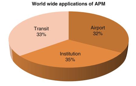
Personal Rapid Transit and Its Development. Figure 2 Distributions of APM applications (Based on data by Fabian 2010 [1])

have initially known each other; Donn Fichter and Edward O. Haltom. Donn Fichter, a transportation graduate student in Chicago, IL, and Edward O. Haltom, a Dallas, TX, contractor who was working on a monorail system. Mr. Fichter sketched a system called Veyar and gradually developed a systems concept integrated into a city with the essential PRT ideas, although he was not a technician. He published a book in 1964 titled Individualized Automated Transit and the City [6]. Mr. Haltom saw a way to "improve" the monorail system that he was working on (that has been in existence since the first monorail constructed in St. Paul, Minnesota in the 1880s) by thinking of smaller guideways and smaller vehicles and invented the monocab. This system eventually became a full-scale test track in California with a totally new switching system owned by Rohr Corporation where linear induction propulsion was added to the system. The patents were purchased by Boeing and the transit system continued to be developed by UMTA (Urban Mass Transportation Administration) Advanced Group Rapid Transit until the mid-1980s.

General Motors Research Laboratories had been working for the military in the late 1950s and created a system that could become public transit, called Hovair. They formed a corporation called TTI, Inc, Transportation Technology Incorporated. A full-scale testing occurred in Detroit in 1969 and the company was eventually owned by Otis Elevator. A second test track was built in Denver. The system was a combination of air-suspension and the linear induction motor and was implemented at Duke University Medical Center. Otis also constructed several cable-drawn versions of this system.

William Alden, a graduate of the Harvard Business School invented, built, and drove a small electric vehicle that could be driven on public roads and then link to a guideway. He called it the staRRcar and it is considered the first dual-mode-system and had an on-board switching mechanism. A test track was built in Bedford, Massachusetts in 1968, the Morgantown system was based on this prototype; however a team of professionals was formed to implement the concept at Morgantown, WVA (Fig. 3).

Honeywell also in its military division through the efforts of Lloyd Berggran wanted to create urban transportation that could be competitive with the

Personal Rapid Transit and Its Development. Figure 3 William Alden StaRRcar – dual-mode vehicle (William Alden)

automobile. He also concluded the same set of PRT characteristics. However, due to his background he created an independent "pod" with all the active power and controlling systems as part of the track. His system was called Uniflo and was designed to be in an enclosed tube. A full-scale test track was constructed by Rosemont Engineering.

Jet Rail was designed by George Adams. He designed, built, and operated a system for Braniff Airlines at Love Field in Dallas that was less expensive but similar to Monocab and proved that a lightweight guideway could be successfully constructed. Cornell Aeronautic Laboratories in the early 1960s designed Urbmobile, it was never built but the automatic control technologists were able to show that short headways could provide adequate capacity – safely. MIT in the mid-1960s produced a report call Project Metran that included the PRT ideas and influenced its continued development.

A planning director, Robert J. Bartells, and a public affairs head of a university, Dr. Jarold Kieffer, both seeking to solve real needs of transit movement for large numbers of people, independently came to the same conclusion of the PRT paradigm. Robert J. Bartells was the director of Planning for the City of Hartford, CT imagined the PRT concepts and ideas and explained and supported them as an important planning director. Dr. Jarold Kieffer, as Head of the School of Public Affairs at the University of Oregon while on a vacation at a sky resort also understood the basic concepts of PRT and has been a continual advocate for the development of the technology.

US Government Participation

It was only through the actions of the Federal Government that the first public system was put into place both technically advancing and greatly hindering the PRT vision. Not fully understanding how totally new public-use transit paradigms need to develop if they are to have long-term success, many boasted and believed that a system could be put into place within 2 years – as we had won the race to the moon! Public-transit is a much more complex and integrated effort of many governmental agencies, organizations, and professionals.

Henry S. Reuss of Milwaukee, Wisconsin in the 1960s urged political support for the development of new transit concepts. He participated in the development of the Urban Mass Transportation Act of 1964 where a Section 6 was added focusing on research, development, and demonstration of new systems for people and goods that stated:

" The secretary shall undertake a study and prepare a program of research, development and demonstration of new systems of urban transportation that will carry people and goods within metropolitan areas speedily, safely without polluting the air, and in a manner that will contribute to sound city planning. The Program shall (1) concern itself with all aspects of new systems of urban transportation for metropolitan areas of various sizes, including technological, financial, economic, governmental and social aspects; (2) take into account the most advanced available technologies and materials; and (3) provide national leadership to efforts of states, localities, private industry, universities and foundations [12].

At this time, the US Department of Transportation did not exist; however, the Urban Mass Transportation Act established the Urban Mass Transportation Administration as a unit of the Department of Housing and Urban Development. Seventeen studies were authorized and these became known as the HUD studies and were summarized in a report titled: Tomorrow's Transportation. Two studies were very influential: A study by Stanford Research Institute and the General Research Corporation (GRC) of Santa Barbara. Stanford focused on new concepts from moving sidewalks to PRT to dual mode and their economic benefits while the main focus of GRC was to computer-model "advanced" systems in real cities and compares them to conventional transit.

There was a team of 17 specialists from various fields that contributed to this study identifying Boston, Houston, Hartford, and Tucson. This study strongly favored new systems due to population growth and increased use of automobiles traditional transit could not continue to meet the demand. This work published in an article, in 1969, by Scientific American titled Systems Analysis of Urban Transportation, became a classic for the technology and brought a national commitment to develop new technologies through the voice of Ben Alexander, the chairman of GRC [8–10].

Once the HUD reports had been released The Aerospace Corporation, a not-for-profit corporation created by the United States Air Force, wanted to use aerospace technology to solve urban problems. Dr. Jack H. Irving concluded that working on high capacity PRT was a good focus for their skilled engineers. They invented new devices such as: powering the vehicles with a pair of linear pulsed direct current motors in interaction with permanent magnets in the track. Except at the switching points they used electromagnets resulting in a no-moving parts switch. The motor could be controlled by solid-state circuitry and was very efficient. They also believed that the guideway should have minimal visual impact so the vehicle was supported by two wheels in tandem. They tested this on a scale model. They were able to develop the system to a very advanced state and used computer simulations proving the feasibility of complex short headway networks. They performed analysis for Los Angeles and Tucson and released their work in a book titled: Fundamentals of Personal Rapid Transit, 1978 [3] (Fig. 4).

The Morgantown system was awarded and built during a very complex time for the newly formed Urban Mass Transportation Administration. Most importantly a presidential change took place bringing all new people into a process that they had no history or detailed understanding of. They wanted immediate results along with preventing the collapse of existing transit systems – two competing goals; and of course they were understaffed.

The Development of the Morgantown GRT

The West Virginia University is located in the hilly, snowy mountain valley town of Morgantown in the Monongahela Valley of West Virginia, and its campus is spread between three different sections of the city. Buses transported students through the center of the city along with all other traffic, creating at that time extreme traffic issues. Professor Samy Elias, Head of the Industrial Engineering Department, became aware of PRT and the PRT test tracks and studies. He believed that this could be a solution for Morgantown. Due to the support of the city, the University and the West Virginia congressional delegation money was obtained for a grant to study three systems. The Alden staRRcar was chosen as the appropriate solution for Morgantown. Due to political connections and pressures, this project was taken very seriously. So, with the 1972 presidential election in mind, the new Head of the Department of Transportation, John A. Volpe, stated that by October 1972 the president should be able to ride the system and therefore this became a federal demonstration project and a team needed to be formed. A contract was signed in December 1970 with the Jet Propulsion Laboratory in Pasadena, California, Boeing, Seattle, WA was the vehicle manufacture, Bendix, Ann Arbor, MI the control system supplier and F.R. Harris Engineering Company of Stanford, CT for the design and construction of the guideway. None of these groups had been working on PRT and there was no time for analysis or a learning curve. This of course led to a complicated and difficult outcome costing four times the original estimate as all of their expertise did not fit with the paradigm changing technology. Recently WVU was

Personal Rapid Transit and Its Development. Figure 4 Aerospace Corporation (Reproduced from [11]. With permission)

awarded a Federal Transit Authority grant that will be a part of the funds to upgrade the existing system (Fig. 5).

Expositions and International Conferences

In 1972, UMTA sponsored an international exposition of four different PRT systems called Transpo72. Millions of federal dollars were set aside for the four systems to be constructed and money to be matched by their respective companies after being chosen. The companies were TTI, Monocab, Dashaveyor, and Ford. Each was to exhibit a minimum piece of guideway and one station in hopes to produce requests for capital grants. However, again due to a short time frame, work to improve the technologies took precedence and those attending the Expo did not understand how these systems could provide a better service and successfully integrate into and improve the built environment. While no city was ready to put its own funds into the development of PRT, many cities did want 100% federally funded programs to integrate the new technology. However the UMTA saw their role as one to encourage private investment [14].

Personal Rapid Transit and Its Development. Figure 5 Heathrow PRT system ( Stan Young, Kansas DOT, University of Maryland, Center for Advanced Transportation Technology)

In the years 1972, 1973, and 1975, three major international conferences were held by the American Society of Civil Engineers (ASCE) People Mover Committee and a volume of published proceedings were produced. However, by 1973, attendance had peaked and the organizing committee worked to develop a permanent organization. In 1976 the ATRA, Advanced Transit Association was formed. ATRA held its own conference in 1978 and more research was added to the body of knowledge. In 1988, ATRA published a broadly based technical committee report to further the importance of the PRT concept. ATRA and the ASCE – People Movers Committees – have continued their work producing published proceedings and a journal [15, 16].

Planners' and Architects' Visions

While the visual impact of an overhead track had been identified from the beginning as an important factor in the acceptance of a PRT system, more emphasis was placed on the engineering aspects than exploring the many approaches that could support visual acceptance. Now, due to advanced technology, the first true PRT system is partially on grade and partially on elevated tracks, only where necessary within an airport, while the Mazdar City PRT system in Abu Dhabi, UAE, will be completely under the city with the vehicles on grade – while many lovely integrative solutions can still be explored! Some architects and architectural studies appeared during the 1970s and 1980s such as in the work of Victor Gruen, Paul Rudolph, and Ulrich Franzen.

Paul Rudolph and Ulrich Franzen were sponsored by the Ford Foundation and the American Federation of Arts producing a book in 1974 titled Evolving City – Urban Design Proposals 17. This publication contained amazing drawings and models for New York City including POD vehicle types and drawings that incorporated PRT into an urban setting. Victor Gruen, known as the shopping center architect, in his Fort Worth Central Business District project in 1950, envisioned "small electric vehicles" under the city to allow full access for all people to the city center. He also created the first pedestrian-only street in Kalamazoo, MI, that still exists today. The two concepts of PRT and walking environments have been connected by architects and planners since the beginning of PRT research, due to the ability of PRT to have smaller stations closer together providing a faster, more accessible, and greater choice in destination [3] (Fig. 6). PRT was also understood as a transit system of choice when connecting other forms of transportation such as automobiles and existing longer-haul transit systems (Fig. 7).

In Great Britain, a steering group for the 1963 UK Department of Transport produced with Colin Buchanan as the key author Traffic in Towns [18] that also became known as the Buchanan Report. He was an influential planner and this report discussed how a balance must be found as increasing automobile ownership was going to challenge the urban environment. Four key points were identified, two being: Towns should be created as environmental areas with quality of living coming first and creating a transit system that could offer an acceptable alternative. This balanced, classic, and seminal report is still referred to today in transportation planning and it is this firm, headed by his son Malcolm Buchanan, that has led the PRT initiative at Heathrow Airport.

History/Overview of Systems in Other Countries

In the early years of PRT, the HUD reports generated the interest in understanding and developing PRT systems around the world. Great Britain, Japan, Germany,

Personal Rapid Transit and Its Development. Figure 6 Aerospace Corporation Station placement and walking distance studies (Reproduced from [11]. With permission of

Aerospace Corporation)

Personal Rapid Transit and Its Development. Figure 7 Paul Rudolph and Ulrich Franzen, Evolving City [17]

France, Sweden, and Canada all became involved to some degree in studying and designing PRT systems.

L. R. Blake wrote an article of his own synthesis of what he saw occurring with PRT development in American and designed Autotaxi with the Britishbuilt environment in mind [19]. The company was started as a private venture, sold to Brush Electric and then was funded by the British National Research and Development Board now being called Cabtrack, a true PRT system. The system was being studied in a systematic and complete way through a step-by-step process including a contract to a large British architectural firm to integrate the system into a section of London as reported in the Architects Journal of May 1971. However, after a new election in Great Britain, the Cabtrack program was stopped. The results and reports of this process are of great value and may have contributed to the success of the Heathrow project.

The Japanese had a full-scale test facility operating in 1972 outside of Tokyo with 4.8 km of guideway and 60 vehicles. Operating with a 1-s headway and a fourpassenger vehicle, a 1,000-vehicle network was simulated. Although many planning and costing studies were evaluated including one for the City of Baltimore, MD, in the United States, several design issues had not been fully considered such as the guideway, station design, and cold weather conditions.

In Germany, two companies inspired by the HUD reports were independently working on PRT concepts. They pooled their resources and thoroughly analyzed many alternatives creating a three-passenger cab supported both above and below a track. They used linear induction motors, one on each side of the vehicle and asynchronous control that was more flexible in the real world. A full-scale test facility was in operation by 1973 and was advertised in 1974 as a successful project. Called Cabintaxi, it was studied to be implemented in Freiberg and Hagen, Germany, and was marketed in the United States. The central business district of Indianapolis tested the system. A program to build a demonstration of a 12-passenger version in Hamburg was underway, as well it was a leading competitor for the Downtown People Movers Program in Detroit, MI, sponsored by UMTA, when the economic crisis of 1980 occurred and the German government withdrew its support. Information can be found about this system as some believe its potential still exists today [20].

The French PRT system called Aramis began with Gerard Bardet in 1967 whose patents were bought by Engins Matra, and in 1970 Matra received a contract. Orly International Airport became the place for a fullscale testing, in 1974, the first phase for proof testing was complete and a contract was awarded for a public demonstration in a suburb of Paris. However the system was based on a platoon concept of grouping vehicles and was designed as a ring system around Paris so vehicle size was increased and the project eventually failed; however, the work with berthing vehicles at stations provided the facts to show that loading and unloading at stations did not slow capacity for the entire system. This project was discussed in a book titled: Aramis or the Love of Technology [21] (Fig. 8).

The Swedish City of Gothenburg, since their city was built on solid rock, were facing a problem of how to deal with expanding mass transportation. Excited by the British efforts they did a great deal of research on PRT systems around the world and decided that the

Personal Rapid Transit and Its Development. Figure 8 Aramis vehicle, France (Reproduced from [11]. With permission)

technology was not ready for public deployment, but continued to be interested in the technology as it was continued to be developed. PRT studies have continued to this day in Sweden as they now move closer to an urban application.

Canada also did a comparative study of PRT, conventional highway and transit technology; however they were interested in freight as well as people movement and called PRT "Programmed Modules." In 1973 in Ontario, the Urban Transportation Development Corporation developed a system; however due to other influences, the vehicle was designed for 40 passengers with all that that implied and met with minimal success in reference to the concept of pure PRT.

After Morgantown

In the late 1970s money was appropriated for a study of automated transit including PRT for Indianapolis using the Cabintaxi system developed in Germany. Several different-sized passenger vehicles were tested in this comprehensive study with the result that the smallest vehicle providing the lowest total cost per passenger mile. This system had the support of business, government, and civic organizations. When this project did not proceed into a real-life application, Raymond MacDonald and J. Edward Anderson began a development program in 1981 at the University of Minnesota that was to take into account all prior research and work to develop the "perfect" PRT system, although they concluded that the aerospace PRT system was the "closest to being right" [22].

A company was formed with the assistance of the University of Minnesota and a Chicago company funded the work until 1986, when Dr. Anderson moved to Boston University. Raytheon and local Boston engineers intrigued by the Chicago-Area Regional Transportation Authority (RTA) were seeking a new approach. Two teams were organized developing designs for one to be chosen for an application. This beginning culminated in the RTA selecting the Taxi 2000 system with Raytheon to design, build, and operate the test PRT system in Rosemount, IL. In 1999, Raytheon terminated its work on PRT 2000; TAXI 2000 Corporation bought back its rights and has continued to develop its concept, now called Skyweb Express.

The PRT concept continued with 2getthere in the Netherlands implementing several successful projects, all on grade: three considered GRT and one PRT. The ParkShuttle technology was applied in the Business Park Riviam, the Airport Schiphol, and the Antibes Demonstration. The CyberCab project, a true PRT system, was tested at a public Flower Show – Floriade at Hoofddorph, Netherlands in 2002. Developed by 2getthere, all of these projects were successfully operated and Riviam continues today as a public form of transit. 2gethere is now designing the PRT system being installed as part of the new carbon neutral Masdar City further discussed below [23].

Ford appeared on the PRT scene briefly with a study of a dual-mode system called PRISM that actually is a Program for Individual Sustainable Mobility [24]. This concept had some similarities to the NEV (Neighborhood Electric Vehicle) initiative. It included very lightweight small vehicles that are on a controlled system. It is an all-electric program that would start small in a few cities eventually growing into a national network linking to high-speed rail. The reason for this program was traffic congestion and the data collected by The Texas Transportation Institute of 68 US urban areas. They understood a system like this could increase fuel efficiency, reduce emissions, and be safer as less driver error would occur.

The South Koreans had been working since 1990 on a PRT system called Vectus and in 2005 began collaborating with the Swedish to construct a testtrack in Uppsala, Sweden, that is designed for winter weather application. The test facility passed safety requirements in 2007, had public access to the system in 2008 and now several studies for real projects in both Sweden and South Korea are underway. The testtrack layout has an outer loop of 300 m, allowing speeds up to 12.5 m/s, and a station track of 100 m with a two-berth station. The station track is designed be long enough to allow merge operations at full speed [25].

The British Company ULTra moved forward with its demonstration project in 2002, followed by a feasibility study in 2004, for implementing PRT at Heathrow airport and is now our first "pure" PRT system in operation. A more detailed discussion follows [26].

Personal Rapid Transit versus Existing Transportation

In understanding the paradigm-changing value of the modern pure PRT to the transportation field, a comparison of PRT to existing systems is crucial. This chart initially from Wikipedia has been adapted for this entry [27]:

Personal Rapid Transit versus Existing Transportation

Similar to automobiles	● Vehicles are small – typically two to six passengers ● Vehicles are individually used, like taxis, and shared only with the passengers of one's choosing ● On-demand, around-the-clock availability ● Travel is point to point, with no intermediate stops or transfers
Similar to trams, buses, and monorails	● A public amenity (although not necessarily publicly owned) shared by multiple users ● Passengers embark and disembark at discrete and fixed stations ● Can be elevated or use air rights over existing highways – reducing land usage and congestion
Similar to automated people movers	● Fully automated, including vehicle control, routing, and collection of fares
Distinct features	● Vehicle movements are coordinated, unlike the autonomous human control of automobiles and bikes ● Reduced local pollution (alternative energy sources such as electric power and solar) ● Small vehicle size allows transit infrastructure to be smaller than other transit modes ● Vehicles travel along a network of guideways where interconnection and multiple station options are standard

Current Systems in Operation or Under Construction

Currently, two GRT networks are operational, one PRT system is operational, one PRT in testing, one full-PRT network is under construction, and several more are in various stages of upgrade, planning, and design. Again the chart is adapted and updated from Wikipedia [27].

In the United States many cities, towns, and activity centers are in various stages of planning with San Jose, CA, and Ithaca, NY, currently leading the way. San Jose is working through a municipal process while Ithaca, NY is studying PRT through a NYSERDA research grant. Alameda Point, CA, Mountain View, CA, Santa Cruz, CA, that is attempting a solar powered system and Fresno, CA, November 2006, the citizens voted to spend \$36 million to establish a fund to begin a PRT effort in their downtown and is currently in the study phase, the others are in various stages of the process. Tysons Corner, VA, and Amber Glen, OR, are all also looking at PRT. In England, Bath, Cardiff, and Corby have been studied for PRT implementation. While in the United Arab Emirates, capital city Dubai, Lulu Island, Abu Dhabi, and Bawadi, Dubai, all are considering PRT systems. Several studies are beginning in India and other European countries. The technology is now being understood for its benefits to people around the world [28].

					Stations/
Location Morgantown, West Virginia, USA	Status Operational	System WVU PRT	Date 1975	Guideway 13.2 km	vehicles 5/73	Notes Up to 20 passengers per vehicle, some rides not point to point during low usage periods
Schiphol Airport Amsterdam, Netherlands	Temporarily operational	Park Shuttle	1997–2004	2,000 m 2 loop network	10/4	Connection from parking to airport 24/7 operation
Rivium Business Park	Operational	Park Shuttle II	1999-today	18,000+ m	8/6	Public Transportation to Business Park and City Functions 20 passengers
Hoofddorp, Netherlands	Temporarily operational	CyberCab 2GetThere	2002	700 m	2/25	Four passengers, transport to view a flower show from a hill peak 40 m high
London Heathrow Airport, UK	Construction completed, open to public	ULTra	2010	3.8 km	3/18	Will be the world's first true commercial PRT system, initially connecting Terminal 5 with a long-term car park. If successful, BAA plans to extend it throughout the airport
Hospital Rovisco Pais, Portugal	Construction completed, under testing	Critical Move	2010			The Hospital Rovisco Pais, a center for physical rehabilitation, uses the Move between the several buildings of the hospital
Masdar City, Abu Dhabi, UAE	Under construction	2getthere	2011	Magnets in pavement, automated driving	83/2,500	Automobiles will be banned, the only powered transport will be PRT and intercity light rail
Suncheon, Republic of Korea	In planning	Vectus	2013	5 km (3.1 miles)	?/40	Will connect Suncheon to the future site of the International Gardening Festival

Heathrow Airport PRT

Heathrow Airport ULTra PRT will be the first "true" PRT project for public use. It has already won a prestigious UK award for transit technology advancement and has been called one of the 20 proven ways to save the earth by the UK Times and also a Sustainable Form of Transport by the Directorate General for Energy and Transport of the European Union.

Heathrow is the main international airport in the UK and one of the busiest in the world. The airport is committed to PRT as the solution to provide connectivity within a very complicated airport system. The initial application and the pilot program connected Terminal 5 with a businessman's parking lot. A higher cost to park can be applied to the businessman as the dramatically reduced time for them from car to terminal is well worth it (Fig. 9).

The initial system is a 3.9 km (2.4 mile) single guideway connecting three stations. Having 21 vehicles to travel between the stations takes about 5 min. The system had to be constructed over a very complex site that included two rivers, seven roads, green-belt land as well as complex airport conditions. If this initial application is successful then it will be extended to include a full network of 350 vehicles, 50 stations, and 30 km of track linking all airport private and public functions [29].

The ULTra pods can hold four adults and two children and can easily accommodate wheelchairs, bicycles and safely carry those who are physically challenged. The pods are battery controlled by a system on the pod. They will save 70% of energy compared to cars and consume less than 50% of traditional buses [30]. The cost in comparison to light rail and transitional

Personal Rapid Transit and Its Development. Figure 9 Heathrow Airport PRT Phase One (Martin Lowsen of ULTra)

	\$m/mile
Automatic People Movers ("APM")	30–100
Light Rail	20–40
ULTra	10–15

Personal Rapid Transit and Its Development. Figure 10 ULTra: PRT sustainable transport (Martin Lowsen of ULTra)

Personal Rapid Transit and Its Development. Figure 11 Two Heathrow Station Design (Martin Lowsen of ULTra)

automatic people moves is quite less, while a traditional bus could be less expensive, the level of service and benefits provided to the community cannot be compared (Figs. 10–12).

Hospital Rovisco Pais, Portugal

This is a PRT system for a hospital setting so that all within the complex have equal access to full mobility – PRT is perfect for this. It is a fully automated electric vehicle, on demand and point to point within a dedicated right-of-way. The user can have communication with the system operator while in the vehicle and can also control the position where the vehicle stops. The vehicle can accommodate eight passengers.

Key Sustainable/Energy and Planning/ Architectural

Being able to synergize transportation, energy, planning, and architecture to meet sustainable goals is a rare confluence of technology/people interconnections. PRT has always been understood for its benefits in minimizing energy usage, while also providing the opportunity for the system to be designed connected to other sources of energy, new planning strategies and architectural design. Peter Calthrope, a Yale-educated architect and sustainability advocate from the 1976 calls it "The ideal transit technology: (a) stations right where you are, within walking distance, (b) no waiting." He has been the supporter of the Alameda Point Project since 2008 especially with the discussion of an additional 60,000 housing units to the area. He

Personal Rapid Transit and Its Development. Figure 12 Heathrow expansion (Martin Lowsen of ULTra)

advocated ULTra PRT as it would enhance carpooling and other forms of transit by allowing all of them to interconnect. PRT can also extend bicycle commutes and enhance walkable community design. At Alameda Point, PRT can assist with interconnections along the Red and Orange lines between Fruitvale BART, Downtown/Park Street shopping, Marina Village jobs, College of Alameda and Rapid Bus transfer, Alameda Point 53-acre Sports Complex, Alameda Point National Wildlife Refuge, Bridgeside Shopping Center, Alameda Point cafes and parks, and Fruitvale Shopping Center.

Suncheon, Republic of Korea

Vectus, a company founded in South Korea that teamed with the South Koreans to construct a test track in Uppsula, Sweden, is now in the planning and design phases for a project in Suncheon, S Korea. The PRT system was chosen to be constructed at the famous Suncheon Coastal Wetlands Park. It marks the first time that the governmental agency has chosen PRT over conventional transit and the environmental reasons could not be more appropriate. Including all of the characteristics that have been mentioned throughout this paper, the South Koreans chose it because it was less costly to build, takes less than half of the construction time and emits no pollutants including CO2 [31].

The first phase of the system will connect the parking lot to the entrance of the wetlands and will contain 40 vehicles on a 5 km system. Mr. Dong Hee Lee, President and Chief Investment Officer of POSCO stated: "POSCO is on the forefront of the global efforts to protect the environment while improving the quality of life". The City will host the International Garden Expo in 2013 and there are hopes that the initial system may even be expanded by this time to connect with the Central Train Station and the city's downtown.

Masdar City, Abu Dhabi, UAE

Masdar City has been under development as the world's first zero-carbon city. This entire 6² km city is completely new and has been totally designed from scratch so that every decision is based upon creating a living place that interacts with its local environment without adversely changing it while also improving the lives of the people who live there. Recently – at the 2009 World Future Energy Summit – the cyber taxi by 2getthere was acknowledged as one of the key features in creating such an environment. They have anticipated 3,000 electric cars with 90 stops connecting light rail, parking, and linking to strategic walking points to the city above. They will operate 24 h a day. The vehicles can travel at 40 kmph and are guided by magnets imbedded in the streets that interact with an onboard navigation system.

It is anticipated that the longest trip by PRT around the city will take no more than 10 min. The city is raised on a podium with all of the vehicles running below the pedestrian-friendly city. The PRT system is anticipated to eventually have 3,000 vehicles serving 130,000 trips/ day. The PRT system will also operate freight delivery to the whole city – FRT (Freight Rapid Transit). The FRT is designed for 5,000 trips a day. Renewable energy in the form of lithium phosphate batteries allow the vehicles to be charged at the stations and will only require a 1.5 h charge for 60 km of use.

Masdar City and 2getthere have the exclusive rights to apply the FROG-technology, the supervisory planning and control system TOMS, as well as unique proprietary subsystems and components (such as the FrogBox and Magnet Ruler – MMS) and a number of related patents for Automated People Mover Systems. These are the technologies that allow this system to run on grade and they have a track record of 22+ years [32].

" The FROG (Free Ranging On Grid) technology creates intelligent vehicles that can operate in any environment. The on board FROG-box® controls the vehicle based on electronic maps (route planning). While driving, the vehicles measure distance and direction traveled by counting the number of wheel revolutions and measuring the steering angle (odometry). External reference points (magnets embedded in the road surface) are used to correct possible small inaccuracies in reference to the planned route (calibration). The reliability of the navigation system has been proven in all previous applications realized and tested successfully by TNO during the FMECA safety-procedure for the ParkShuttle Rivium application that has been operating since 1999.

San Jose Airport, San Jose, CA

The City of San Jose has identified the area around the Sam Maneta airport as a place where the PRT concept can assist with linking all of the existing movement systems such as Caltrain, BART, and VTA Light Rail as well as potentially connecting to other places not directly related to the airport such as North San Jose, as well as to new growth. They have earmarked \$4 million to conduct two simultaneous studies, one technical and the other with a focis on transportation and urban planning. Laura Stuchinksy, a sustainability officer for the San Jose Department of Transportation and many other city officials see PRT as a complement to all of these systems and one that will allow all of them to function as a complete transportation system for the airport and local area – a circulator system interconnecting all the systems. This was noted in a paper by Young, Miller, and McDonald. In September 2008, they issued the initial request that is now in the final contract negotiation phase. They expect to have an operational system by the end of 2015 (Fig. 13).

The following is an excerpt from the City of San Jose:

" It will start with a limited demonstration project and proceed in three phases:
- Phase 1: Preliminary Design A determination of feasibility as described above.
- Phase 2: Final Design Selection of system design and construction contractor(s); completion and verification of detailed design.
- Phase 3: Construction, Integration and Testing Physical construction of the system on-site culminating in operational certification.

All typical analysis for transportation infrastructure such as ridership forecasts, routing determinations, architectural development, civil engineering design, environmental impact assessments, and community outreach will be a part of the process. While nonconventional aspects of this project include new usage and operational models, completely new civil architectures and their

Personal Rapid Transit and Its Development. Figure 13 Conceptual comparison of modes in the accessibility – throughput spectrum from Young, Miller, McDonald. Keys to innovative transport development. Presented at the 87 Annual Meeting of the Transportation Research Board, Washington, DC, 2007

integration with the as-built environment, along with new elements of the technical system – innovative designs for propulsion, control, vehicles, guideways, and vehicle management systems, for example, that may be selected, are specified and arranged in various ways to provide varying degrees of utility and capability.

New approaches and guidelines/standards may need to be developed, as will ridership forecasting and performance evaluation models. A thorough review of technical capabilities and maturity level relative to the resulting performance requirements is required as is an assessment regarding the ability of the still-small vendor base to deliver such systems.

The CITY has selected two consultants as project advisors, The Aerospace Corporation (SYSTEMS CON-SULTANT) and Arup North America Limited (TRANS-PORTATION CONSULTANT). In general, TRANSPORTATION CONSULTANT will address all conventional transportation infrastructure issues. SYSTEMS CONSULTANT and TRANSPORTATION CONSULTANT will together address the unconventional project issues; the TRANSPORTATION CONSULTANT focusing on the civil infrastructurerelated items and the SYSTEMS CONSULTANT focusing on the technical system, as described generally above.

General Approach The two consultants will work collaboratively as part of an Integrated Project Team (PROJECT TEAM) led by the CITY. They will share information and provide input necessary to each other's work and project deliverables, integrating their workflows to achieve the CITY's project objectives [33].

Future Directions

High-Tech/Low-Tech Connections: Man and Machine

As PRT becomes more available for public use, the positive connections between technology, the environment, our communities, and ourselves – the low-tech/High-tech connectionwill be better understood and allowed to flourish. What are the high technologies of the future and how are they transforming the ways that we travel through space, place, and time. The test is how many lives can be

| The Basics of Several PRT Systems | | | Seating
Capacity | | | | |---------------------------------------------|---------------------------|---------------|------------------------------------------------------------------------------------|-----------------------------------------------|--|--| | System
Morgantown PRT (Boeing) | Location
West Virginia | Active
Yes | Status
In service | (per vehicle)
8 seated plus
12 standing | | | | ULTra (ATS Ltd) | UK | Yes | In testing for final commissioning | 4 | | | | Critical Move | Portugal | Yes | In on-site testing | 4 | | | | 2getthere PRT | Netherlands | Yes | 10 vehicles produced for Masdar City | 6 | | | | Vectus PRT (POSCO) | South Korea | Yes | Full prototype, Sweden; Suncheon, Korea | 4 | | | | Cabinentaxi [24] | Germany | No | Completed system: 1980s approval for
federal transit programs in Germany and US | 3,12,18 | | | | PRT2000 (Raytheon) | USA | No | Full prototype | 4 | | | | Skyweb Express (Taxi2000) | Minnesota | Yes | Partial prototype | 3 | | | | MISTER | Poland | Yes | Partial prototype | 5 | | | | JPods | USA | Yes | Mockup | 4 | | | | SkyTaxi | Russia | Yes | Concept | 1,2,4 | | | | Launchpoint Technologies
SPM Maglev [25] | USA | Yes | Concept | ? | | | | Skycab AB Skycab | Sweden | Yes | Concept | ? | | | | SkyTran Unimodal | USA | Yes | Full scale prototype | 3 | | |

transformed for the better, for greater accessibility and the long-term sustainability of our planet – these technologies should be explored, developed, and expanded.

PRT with automated transit technologies will continue to evolve to become a greater part of our future built world. They have the ability to transform the way that we design and build our places for living, just as positively as the car did over 100 years ago. Following that technological innovation many peoples lives were changed and for the betterment of all. Since the late nineteenth century, world's fairs have offered futuristic visions of how people could and would live. Automated People Movers are among the visions that have become reality from them. Although most people connect monorails with world's fairs and amusement parks, there is no reason to limit advanced transit technology to such environments. For many land uses – such as airports, medical centers, and colleges – automated people movers have tremendous potential to address congestion, increase connectivity, mitigate parking shortages, and provide links to parking and PRT has the most potential within this category to really transform our lives.

Because of its human scale, PRT allows the pedestrian experience to be preserved – minus the traffic and congestion. It can also provide a more flexible link between man and machine: because it so small, quiet, and light (compared with conventional transit), PRT can be adapted to a wider array of environments. Although PRT does not eliminate the need for parking in many situations, it does offer opportunities to change the parking paradigm. In an automated parking facility, for example, PRT vehicles could easily change direction or move between levels within a small space [34].

PRT systems can provide excellent transit coverage for urban or suburban areas; such a systemwould be ideal, for example, in locations such as Destiny USA – the environmentally sensitive entertainment, shopping, and technology project in Syracuse, New York. PRTwould be equally appropriate in more traditional urban locations, particularly as a link between parking and other land uses. As part of a larger effort to explore the transformation of office parks into transit villages, Cities21, a nonprofit research organization based in Palo Alto, California, is completing an EPA-funded study of the environmental benefits of a PRT system within the Hacienda Business Park [35].

In the 1960s, William Alden designed the StarrCar, a vehicle that could function independently, on the road, or on dedicated tracks, as part of a transit system. At the time, technology had not yet caught up to Alden's vision, although part of Alden's concept was the basis for the Morgantown PRTsystem. Today, however, with advanced automotive technology, Alden's vision is almost within reach. Within a system that allowed vehicles to be taken off the tracks as needed, for example, PRT vehicles may be used to pick up drivers at their parking spots and take them to their next destination. The parking facility could both provide space for traditional vehicles, and become an active participant in new approaches to transit and movement! (As automotive technologies advance, moving in the direction of "cars that drive themselves," it may be possible to drop off a car at a garage and have the car park itself as you connect to the PRT system. As PRT, automated vehicles, and other high-tech transportation options become integrated into the overall transportation system, they will affect parking garage design in ways that cannot yet be imagined [36]).

Beauty, technology, function, engineering, and civic purpose: the pieces are all in place. But determining the solutions of the future – whether urban, suburban, or rural – will mean connecting, at a deeper level, to the ways in which people relate to the world around them. It will be through these deeper connections that new solutions emerge. Horst Bredekamp, in an exploration of the phenomenon of the Kunstkammer – the cabinets of art and curiosities that were the precursors to modern museums – notes that

" No one wants to return to the deliberate chaos of the Kustkammer as museums. But the boundaries between art, technology, and science are beginning to break down in a similar manner as has been demonstrated by the Kunstkammer. In view of this fact, their lessons of visual association and thought processes which precede language systems take on a significance which might even surpass their original status. Highly technological societies are experiencing a phase of Copernican change from the dominance of language to the hegemony of images [36].

In looking toward the future of PRT, advances in new transit technology have been hindered by a lack of focus on research and development in this area. However, in fits and starts, and often with private money and due to the perseverance of innovators and visionaries, PRT is just starting on its path to its full potential, finding its way into our world of public transit linking with all existing forms of movement.

One of key area of future advancement is the control software that allows for flexibility and openness so that the complex and time-consuming tasks that will allow a large fully operational city PRT system to function safely and quickly can be applied to public transit. Systems of this type are being implemented in Automated Guided vehicles for warehouses and manufactures as well as being used successfully in airport luggage systems and emerging PRT systems.

The motivation behind PRT is to provide not just an advanced commuter transit experience but to provide a type and level of service that meets the needs of those who cannot or do not have access to the automobile, a truly new way to move and live in our modern world. It is a transit system that attempts to put people and cities first through technology while making an improvement to the quality of urban life.

The theory and reality of PRT shows this technology to be the transit technology of the future. From 2002 to 2005 the EDICT project funded by the European Union and involving 12 research organizations concluded that PRT [37]:

Would provide future cities "a highly accessible, userresponsive, environmentally friendly transport system which offers a sustainable and economic solution"
Could "cover its operating costs, and provide a return which could pay for most, if not all, of its capital costs"
Would provide "a level of service which is superior to that available from conventional public transport"
Would be "well received by the public, both public transport and car users"

The risks of being the first to implement the system are being removed and so we should see the technology move forward and provide the level of service to all users of transit that has been envisioned since its beginnings. A review of all of the literature shows many detailed specific studies about networks, walkabilty, systems concepts, human affect, and proposals that indicate all that is claimed about PRT is real so now according to Rachel Liu [1] all that is required are:

" multiple business models so that its many applications can find funding. As concluded in a recent PRT study (Carnegie and Hoffman 2007), AGT possesses the virtue of sustainability due to its small footprint, lower cost and lower impact on the environment. On the other hand, its small size and low-key profile have fostered a large number of applications worldwide without garnering any major headlines, which may, however, suppress its potential as a unique solution to urban circulation and congestion problems.

Along with:

on-going PRT studies reveals that the specifications of technology and assessment of costs may be relatively straightforward, but quantifying benefits associated with the implementation of a transportation project and evaluating the market conditions are complex. There are a number of analytical tools to assign a dollar value to benefits; however, some impacts such as congestion relief, safety improvements, or air quality improvements are often difficult to quantify financially. Other qualities, such as aesthetic appearance, may not even be quantifiable. Environmental and societal impacts are often referred to as "external" effects of transportation activities since they are not directly reflected in monetary costs and benefits of project implementation. By externalizing these factors, benefit/cost analyses often do not capture the full value of beneficial impacts. However, the significance of all impacts, both positive and negative, needs to be considered in the decision-making process.

Bibliography

Primary Literature

1. Liu R (Rachel) (2010) Spectrum of automated guideway transit (AGT) technology and its applications. In: Kutz M (ed) Handbook of transportation engineering. McGraw-Hill, New York
2. Committee of Automated People Mover Standards (2006) Automated people mover standards, Part 3. American Society of Civil Engineers, Reston
3. Irving J (ed) (1978) Fundamentals of personal rapid tansit. DC Heath, Lexington
4. Morgantown PRT: http://transportation.wvu.edu/prt
5. Gunter M (7 Mar 2008) Building the world's cleanest city. Fortune Magazine
6. Fichter D (1964) Individualized automated transit and the city. BH Sikes, Providence, RI
1. Anderson JE (1996) Some lessons from the history of personal rapid transit. Paper presented at the international conference on personal rapid rransit (PRT) and other emerging transportation systems, Minneapolis, Minnesota, 18–20 Nov 1996. http://advancedtransit.org/doc.aspx?id=1025
8. Cole LM, Merritt HW (eds) (1968) Tomorrow's transportation: new systems for the urban future, US Department of Housing and Urban Development, Office of Metropolitan Development Chapters available online: "Summary," pp. 1–5; "Recommended Future Systems," pp. 58–77. http://faculty. washington.edu/jbs/itrans/tomtran.htm.
1. Henderson C et al (1968) Future urban transportation systems: descriptions, evaluations and programs, Final report, Volumes 1 and 2. Prepared for the US Department of Housing and Urban Development by the Stanford Research Institute
1. Systems Analysis of Urban Transportation Systems (1969) Scientific American 221:19–27
1. Burke C (1979) Innovation and public policy: the case of personal rapid transit. Lexington Books, D.C. Heath
1. Andreasson I (2000) Innovative transit systems, VINNOVA: Swedish Agency of Innovation Systems. http://vinnova.se/ publ/list\_vr.htm#03 as well as Vectus web site http://www. vectusprt.com/
1. Lowson M ULTra Urban Light Transport, Advanced Transport Systems. http://www.atsltd.co.uk/
1. United States Congress, Office of Technology Assessment (June 1975) Automated guideway transit: an assessment PRT and other new systems. US Government Printing Office, Washington, DC
1. Merritt HW (1993) Reflections on the New Systems Study Project, pp 35–59 in Automated People Movers IV: Proceedings of the 4th international conference on automated people movers, American Society of Civil Engineers, Irving, Texas, 18–20 Mar 1993. http://faculty.washington.edu/jbs/itrans/reflec2.htm
1. US Congress, Office of Technology Assessment (June 1975) Automated guideway transit: an assessment of PRT and other new systems. Prepared for the Senate Committee on Appropriations, Transportation Subcommittee. http://ntl.bts.gov/ data/OTA/7503/7503.htm
1. Wolf P (1975) Evolving city. American Federation for the Arts, New York
1. Reports of the Steering Group (1963) Traffic in towns. H.M. Stationery Office, London and reprint Penguin Books in association with HMSO
1. Blake LR (1966) A public transport system using fourpassenger, self-routing cars, Inst. Mech. Eng. convention on guided land tTransport, vol 181, Pt. 3 G
1. Tadi R, Utpal D (1997) Detroit downtown people mover: ten years after. paper presented at the 6th international conference on automated people movers, Las Vegas, NV
1. Latour B (1996) Aramis or the love of technology. Harvard University Press, Harvard
1. MacDonald R, Anderson JE (1978) Transit systems theory. Lexington Books, D.C. Heath. 21st century personal rapid transit, Self-publish
1. 2getthere: http://www.2getthere.eu/
1. Proposal for Independent Sustainable Mobility (PRISM) (pdf). Ford Advanced Research Division (2003) http://faculty. washington.edu/jbs/itrans/PRISMGPCPaper.pdf. Accessed 3 Aug 2010
1. http://www.vectusprt.com/
1. Heathrow airport web site: http://www.heathrowairport.com/ portal/controller/dispatcher.jsp?CiID=e993760079e1d110 VgnVCM10000036821c0a\_\_\_\_&ChID=10b35109350d3110 VgnVCM10000036821c0a\_\_\_\_&Ct=B2C\_CT\_PRESS\_RELEAS E&CtID=a22889d8759a0010VgnVCM200000357e120a\_\_\_\_ &ChPath=Home%5EHeathrow%5EHeathrow+press+releases
1. http://en.wikipedia.org/wiki/Personal\_rapid\_transit 28. Multiple website concerning PRT http://www.princeton.edu/
alaink/Orf467F04/NJ%20PRT%20Final%20Small.pdf 29. Lowson M (2004) (doc) A new approach to sustainable transport systems. 13th World Clean Air and Environmental Protection Congress London, 22–27 Aug 2004. http://www.ultraprt.
1. Rodgers L (2007) Are driverlss pods the future. http://news. bbc.co.uk/2/hi/uk\_news/7148731.stm. Accessed Aug 2010
1. http://www.vectusprt.com/center/news\_view.php
1. Masdar: http://www.masdar.ae/en/home/index.aspx
1. San Jose: http://www.sanjoseca.gov/transportation/Support Files/admin/RFI\_Auto mated\_transit\_networkQA.pdf
1. Cities21: http://www.cities21.org/cms/

com/media/papers/

35. McDonald S (2007) The parking garage: design and evolution of a modern urban form. Urban Land Institute, Washington, DC
36. Bredekamp H (1995) The lure of antiquity and the cult of the machine: the Kunstkammer and the evolution of nature, art, and technology. M. Wiener Publishers, Princeton, pp 113
37. EDICT: EDICT Final Report (pdf) from cardiff.gov.uk

Books and Reviews

Advanced Transit Association (1988) Personal rapid transit: another option for urban transit? J Adv Transport 2(38):192–314
Anderson JE (July 2009). An intelligent transportation network system: rationale, attributes, status, economics, benefits, and courses of study for engineers and planners. PRT International, LLC
Anderson J, Romig S (1974) Personal rapid transit II. Audio-Visual Extension, University of Minnesota, Minneapolis, MN
Carnegie JA, Hoffman PS (2007) Viability of personal rapid transit in New Jersey. New Jersey Department of Transportation, New Jersey, 141p
Institute for Transportation in Cooperation with the Advanced Transit Association (1966–present) Advanced Transport Quarterly, Wiley-Blackwell
Muller P (2007) A personal rapid Transit/Airport Automated People Mover Comparison" Proceedings of the 29th international air transport conference. American Society of Civil Engineers. http://www.prtconsulting.com/
Richards B (2001) Future transport in cities. Spon Press, London Schneider JB (2011) Innovative Transportation Systems. This web site offers a wealth of information, including summaries and excerpts from many other sources of information. http:// faculty.washington.edu/jbs/itrans/
Warren R (1998) The urban oasis: Guideways and greenways in the human environment. McGraw-Hill, New York

PHEVs and BEVs in Coupled Power and Transportation Systems

MLADEN KEZUNOVIC¹ , S. TRAVIS WALLER² 1 Department of Electrical and Computer Engineering, Texas A&M University, College Station, TX, USA 2 Department of Civil Engineering, The University of Texas at Austin, Austin, USA

Article Outline

Glossary Definition Introduction Policy Issues Modeling of Complex Systems Benefits Conclusions and Future Research Acknowledgments Bibliography

Glossary

BEV Battery electric vehicle.

DSM Demand side Management; utility-sponsored programs to influence the time of use and amount of energy use by select customers.

G2V Grid-to-vehicle; using the electrical grid to charge the battery of a vehicle.

HEV Hybrid electric vehicle.

OM Outage management; set of manual and/or automated procedures used by operators of electric distribution systems to assist in restoration of power.

PHEV Plug-in hybrid electric vehicle.

V2B Vehicle-to-building; exporting electrical power from a vehicle battery into a building.

V2G Vehicle-to-grid; exporting electrical power from a vehicle battery to the electrical grid.

Definition

With the price of oil peaking in the recent past close to the once unimaginable \$150 per barrel and the threat of global climate change increasingly acknowledged, the transportation sector is employing a number of new technologies that will enhance energy security by reducing the current dependency on oil-based fuels. Should the gasoline cost increase in the future, Plugin Hybrid Electric Vehicles (PHEVs) and Battery Electric Vehicles (BEVs) will become the economical choice for transportation. Widespread adoption of PHEVs/ BEVs will also improve air quality and carbon footprint, since point source pollution is easier to control than mobile source pollution. This level of control is essential for effective implementation of carbon capand-trade markets, which should spur further innovation. In USA, sales of Hybrid Electric Vehicles (HEVs) have grown 80% each year since 2000, proving that PHEVs/BEVs are likely an eventual reality that must be dealt with [1]. The implications of this reality will be highly dependent on the policies in place to use PHEVs/BEVs to the benefit of the transportation and power systems, as well as the drivers, industry, and public at large.

Beyond fuel costs and sustainability, the primary concern of the transportation sector is congestion. In 2005, congestion was estimated to cost the US economy \$78.2 billion in wasted time and fuel [2]. If PHEV/BEV drivers are given appropriate incentives (e.g., strategically placed energy exchange stations), traveler behavior (e.g., choice of routing, departure time, and destination) impacting congestion may be affected.

In addition, the power industry is currently challenged to maintain reliability of operation while expanding the grid to meet growing demand. Large blackout such as the northeastern one in 2003 may create loses in billions of dollars [3]. Introducing the renewable resources to meet growing demand requires energy storage to deal with interfacing [4]. If proper policy is in place PHEVs/BEVs can provide a promising solution acting as mobile decentralized storage (MDS) of electrical energy. In this capacity, PHEVs/BEVs can serve in two modes: grid-to-vehicle (G2V) and vehicleto-grid (V2G), each providing benefits to the power system operation. The G2V mode can be used to charge PHEVs/BEVs at reduced cost when the power system load is reduced and generation capacity is abundant, such as during night time. The V2G mode may be used when demand is high or supply is accidentally lost since the stored electric energy can be released from PHEVs/ BEVs in an aggregated way, which will offer major contributions to regulation service and spinning reserves, as well as load-shedding prevention. The mobility of the energy storage in PHEVs/BEVs allows for strategic placement of the distributed generation source to optimize power system needs.

Figure 1 illustrates the spatial and temporal coupling of the power and transportation systems through showing an example of a PHEV/BEV driver's route, highlighting destinations where the driver could potentially engage in G2V or V2G activity. Options for meeting selected criteria for electricity and transportation networks simultaneously are numerous. Developing policy strategy requires understanding of trade-offs involved in pursuing certain solutions at the expense of others. The all-encompassing theoretical framework for such studies to the best of our knowledge is not available.

Traditionally, scientists have adopted a divide and conquer approach to understanding complex phenomena. Unfortunately, systems with emergent dynamics that are dominated by contextual interactions are not well suited to this classical approach (e.g., [5–7]). In such cases, directly addressing the couplings of system components may actually hasten progress. While this linkage presents new opportunities to improve the functioning and capacity utilization of each system, it

PHEVs and BEVs in Coupled Power and Transportation

Systems. Figure 1 Temporal and spatial dimensions of plug-in opportunities also raises the spectrum of increasing dynamic complexity and cascading failures across systems.

In this entry, several open policies and research goals will be discussed, which facilitate optimizing the integration of the transportation systems and the behavior of its travelers with the electricity systems and behavior of its end-customers. PHEVs/BEVs based demand side management (DSM) and outage management (OM) are also presented as an application of PHEVs/BEVs using in the coupled power and transport system.

Introduction

The impacts PHEVs/BEVs will have on transportation systems, power systems, and air quality are very complex. Studies conducted to date on this topic make many assumptions to simplify the problem. As stated in the definition, the problem space must be treated as one large complex system in order to capture emergent behavior.

The complexity of the issues involved in studying PHEVs/BEVs and their interaction with electricity and transportation networks is shown in Fig. 2, where several disciplines that need to be involved in researching this multidisciplinary problem are shown.

Recent analyses confirm the feasibility of the gridto-vehicle (G2V) and vehicle-to-grid (V2G) concepts [8–13]. The Electric Power Research Institute

PHEVs and BEVs in Coupled Power and Transportation Systems. Figure 2

Illustration of multidisciplinary nature of problem

speculates that V2G could reduce the requirement for global, central-station generation capacity by up to 20% by the year 2050 [14]. Several studies omit any consideration of vehicle locations and desired activity patterns and assume a percentage of vehicles are plugged in and available when estimating the benefits to the grid and to drivers [8, 10, 11].

Many researchers have investigated the various potential benefits and implementation issues of the V2G concept. Kempton and Tomic´ studied the fundamentals of using PHEVs/BEVs for load leveling, regulation, reserve, and other purposes [15, 16]. Hadley and Tsvetkova analyzed the potential impacts of PHEVs on electricity demand, supply, generation, structure, prices, and associated emission levels in 2020 and 2030 in 13 regions specified by the North American Electric Reliability Corporation (NERC) [17]. Meliopoulos et al. considered the impacts of PHEVs/ BEVs on electric power network components [18]. Anderson et al. performed the case studies of PHEVs/ BEVs as regulating power providers in Sweden and Germany [19]. Guille and Gross presented a proposed framework to effectively integrate the aggregated battery electric vehicles into the grid as distributed energy resources [20]. The combined impact PHEVs/BEVs make on both electric power system and transportation network has not been explored as much. When considering the role of PHEVs/BEVs as dynamically configurable (mobile) energy storage, the potential impacts on both electricity and transportation networks may become quite diverse. The flow of traffic is an important factor in deciding the flow of electric power that could be utilized from PHEVs/BEVs. Correlating the movement of people to the movement of the power load offers new opportunities in the smart grid.

One of the major advantages of PHEVs/BEVs is their usefulness as an MDS. MDS is a revolutionary concept because currently the power grid has no storage except for 2.2% of its capacity in pumped storage [11]. Without significant and reliable storage of energy, maintaining grid stability and reliability under the growing electricity demand is a complex problem. Utilities may contract with others to provide power in any one of the four types of markets: base-load power, peak power, spinning reserves, and regulation services. Several studies have shown that PHEVs/BEVs can provide ancillary services (spinning and regulation) at a profit [8, 10, 11]. Spinning reserves receive payment for providing continuous capacity regardless of whether energy is provided, and receive further payment if called on to feed energy into the grid. Regulation services feed a nominal amount of energy into the grid, and receive payment for reducing or increasing their energy consumption as needed. In the case of PHEVs/BEVs, being plugged-in in a predictable way means that capacity is available to feed into the system if called upon. PHEVs/BEVs are particularly well suited for regulation services since the impact on vehicle's energy resources may be zero.

The pricing of V2G and G2V services is expected to cause a fundamental shift in the behavior of PHEVs/ BEVs drivers. Further research is needed to investigate the exact nature of this shift; however, if the pricing schemes are developed with both the power system and transportation system in mind, then PHEVs/BEVs could help solve problems plaguing the traffic network, particularly congestion. The pricing scheme should also consider air quality impacts caused by charging at different times in the day. As mentioned earlier, MDS will allow for renewable energy to be used more efficiently. There will however remain times of the day more dominated by "dirty" fuels than others.

As observed, the body of research literature related to the multidimensional impact of PHEVs/BEVs is quite small. The remainder of this section will focus separately on the dual problems of improving the stability and reliability of the electrical grid and improving the efficiency of the roadway network.

Stability and Reliability of the Electric Grid

Stability and reliability of the US electric grid have become issues of increasing concern since the occurrence of several blackouts in the 1990s (Western Interconnect in 1994 and 1996, and the Eastern Interconnect in 1999) and system deregulation. The devastating impact of the northeast blackout from August 14, 2003 reminded that the situation with the grid is only worsening and not improving. Here, a stable system is defined as one in which the phase and frequency of power generation units are constant. Ability of the system to maintain the state of equilibrium during normal and abnormal conditions is a measure of

PHEVs and BEVs in Coupled Power and Transportation Systems. Figure 3 Illustration of multidisciplinary nature of problem [21]

stability. Reliability is defined as the ability of the system to meet unexpected demand and respond to failures. Ability of the system to deliver electricity to customers within the accepted standards, which may be affected by the failure rate, repair rate, or duration of loss, is a measure of reliability. Figure 3 illustrates the worsening stability problem. Order 888 in Fig. 3 relates to the Open Access to Transmission issued by Federal Regulatory Commission in 1996, which is the result of an authorization passed by the Congress as a part of the Energy Policy Act of 1992.

A major challenge in achieving these goals (stability and reliability) is the lack of energy storage. Figure 4 depicts the peaking structure of an example power load over the course of 1 day. In this example, demand grows rapidly starting at 6 a.m. and begins to decline after hitting a peak around 3 p.m. This peaking phenomenon is especially important to consider given that different energy sources are available at different times of day. For example, wind energy is most widely available at night when the demand for power is the lowest. While it may seem intuitive that a flat demand curve is the ideal, this is not necessarily true. More research is required to determine if parts of the system (e.g., transformers) require time to cool down. The large scale use of energy storage would significantly help meeting the stability and reliability needs, including managing the load variations shown in Fig. 4.

Efficiency of the Roadway Network

Congestion is a problem not only in the electricity grid network, but also in the roadway network. Vehicle miles traveled (VMT) has risen consistently since the advent of the automobile, with dips when gasoline prices rise quickly (See Fig. 5 for the VMT trend since 1992). If the transportation sector is shifted to an alternative fuel source (i.e., electricity) with greater price stability, and especially if the source of the fuel is renewable, then VMT is expected to continue to increase into the foreseeable future. While mobility is an indicator of economic success, the expansion of a roadway system is limited by available space and finances. Roadway network efficiency is further constrained by the individual autonomy of drivers who act in their self-interest instead of the interest of

PHEVs and BEVs in Coupled Power and Transportation Systems. Figure 4 Illustrative peaking of electricity load [12]

PHEVs and BEVs in Coupled Power and Transportation Systems. Figure 5 US highway VMT [23]

the system (see [22] for a theoretical description of traveler behavior).

Extensive research has been conducted on improving the efficiency of the transportation system via methods such as pricing and technology, but few solutions proposed offer a case even close to being as comprehensive as PHEVs/ BEVs.

Policy Issues

The policy issues presented here are centered on incentives to help industry develop and bring new value to end users of electricity and transportation networks, and society at large, while encouraging competition and development of new business opportunities.

Improve Electric Grid Performance

Widespread deployment of PHEVs/BEVs will allow for increased energy storage, and improved reliability and stability of the electric grid. Linking the transportation and power systems through PHEVs/BEVs will allow for electrical energy storage on a scale much larger than is currently feasible. The additional energy capacity will be directly proportional to the penetration of PHEVs/ BEVs into the automobile market, and modeling (see the modeling section) is needed to determine the exact increase in capacity across the space and time dimensions.

The new mobile storage can only benefit the electric grid if it is available at the right time and place to service the grid when needed. To determine PHEVs/BEVs' demand for electric energy across space and time, travel patterns must be considered. Figure 1 shows an example of such a pattern, highlighting several destinations where a driver could potentially engage in G2V or V2G.

Stability and reliability issues were mentioned earlier. V2G is poised to greatly aid the grid in becoming more reliable and stable because vehicles are only in use for a small portion of each day (average daily travel time person in 2001 was 82.3 min [24]). During the remainder of the day, the vehicles can be plugged in and provide services (e.g., ancillary or regulatory).

This approach requires a policy shift to allow use of the MDS for energy to maintain stability and reliability. Also, policy that encourages utilities to cooperate with the PHEV/BEV owners or aggregators and provide tariff incentives for their participation in programs aimed at demand and distributed generation management and optimization is missing at the moment.

Enhance Penetration of Renewable Energy Sources to Improve Energy Security

Increasing energy capacity by using PHEVs/BEVs as MDS will allow for increased investment in renewable energies by alleviating concerns related to the temporarily highly variable nature of solar (daytime) and wind (primarily nighttime). Using renewable energy has benefits not only for the environment and air quality, but also for energy security by reducing reliance on the supply from oil producing countries.

This approach requires a policy shift to allow and encourage large scale use of the MDS for energy to support interfacing of renewable generation.

Reduce and Redistribute Pollution in the Electric Grid and Transportation Network

By shifting the source of pollution away from vehicles, PHEVs/BEVs will change the transportation-based air pollution problem from a mobile source issue to a point source issue. This redistribution of pollution will likely have the effect of reducing pollution because point sources are much easier to control and some already have emission caps in place. Hadley [25] conducted initial research into the potential air quality impacts of PHEVs/BEVs, describing the impacts of G2V charging on air quality, and considering the types of power generation that are typically used at different times of day (e.g., coal-fired generation is prevalent at night in some regions).

Some policies are already in place to ensure that the redistribution of pollution that will occur with widespread deployment of PHEVs/BEVs will actually lead to a reduction in pollution. Further policy analysis is needed to ensure that V2G and G2V services are incentivized to occur at times when it will result in the maximum improvement in air quality.

Create New Markets and Further Deregulate Existing Markets

PHEVs/BEVs are poised to open new markets and increase opportunities in existing ones. Carbon-trade markets should be aided because they facilitate the change of the transportation-based air pollution problem from a mobile source issue to a point source issue (as described earlier). While point sources of pollution are much easier to control, if they are nonrenewable, they will likely need to trade carbon credits to counter the increased emissions.

PHEVs/BEVs will also create new modes for participation in the electricity markets. There will be opportunities for businesses to act as Qualified Scheduling Entities (QSE) to the electric utility by facilitating V2G/ G2V interactions. Such a QSE that aggregates across vehicles is necessary because any one vehicle's contribution will be too small to allow it to participate directly in the market. PHEVs/BEVs will likely function akin to small generators as a distributed energy resource.

Policy that enhances market development and deregulation allowing a new type of QSE to bid in a variety of markets is needed to facilitate the aggregated use of PHEVs/BEVs in "transportation-energy" markets.

Plan and Develop Energy Exchange Stations

Energy exchange stations (for G2Vand V2G) could take one of at least two forms. The first, the way considered by most electric vehicle research to date, assumes that individual drivers plug in and charge their vehicle over a period of several hours. Some examples of potential charging station locations are shopping malls, recreational areas, schools, and of course homes.

Further, rather than requiring drivers to plug into the grid and wait several hours to charge their batteries, battery exchange locations could be as ubiquitous as gas stations and automatically exchange discharged batteries with fully charged batteries. Charging PHEVs in this way has benefits for drivers because the process takes only a few minutes as opposed to several hours. Also, this system would require a leasing system for batteries similar to the system in place for leasing cell phones, alleviating driver concerns about battery life. The benefit for utilities is that control over charging and servicing the grid is centralized.

In reality, charging (G2V) and discharging (V2G) services will likely be based on a hybrid of the two methods mentioned above (individual drivers plugging into the grid and stations designed to exchange batteries). Depending on the pricing structure in place, it may make sense for drivers to exchange batteries during long drives and plug in to a household plug at night. Incentive structures will need to be developed that consider the different players – energy exchange stations and individual drivers.

The temporal and spatial aspects of the activity patterns travelers choose (see, e.g., Fig. 1) adds a layer of complexity to the problem of locating charging stations to link the transportation and energy systems. This requires both micro (neighborhood, city, and metropolitan area) and macro (region, state, and nation) driver behavioral dynamics to be studied in detail. If appropriate incentives are developed, drivers could be encouraged not only to act in a way that best serves the grid, but also to act in a way that best serves the transportation system. The incentives could be passive such as pricing electricity for planned contribution at the location of charging facilities (either stations or induction charging embedded in the roadway), or active such as pricing electricity based on congestion in both the power grid and local transportation system. Cognitive and behavioral research is needed to determine the appropriate incentives.

Policy that addresses the planning requirements for charging stations and regulates emerging energy exchange markets is needed. Comprehensive policy that develops joint electricity and transportation programs for incentivizing drivers to participate in the transportation and electricity grid optimization are not yet proposed or even clearly defined.

Modeling of Complex Systems

To develop policy strategies that allow for faster and more significant penetration of PHEVs/BEVs, research is needed to model the interactive performance of two complex systems, power and transportation, linked through the behavior of individual vehicle operators, where this linkage is determined by the location of interface infrastructure. The behavior of travelers defines the required inputs into power modeling since time-dependent PHEVs/BEVs locations are critical. Every aspect of this meta-system enterprise (power, transport, consumer choice, and infrastructure development) is interlinked, therefore fully understanding policy issues is quite challenging. This section explores each aspect of the modeling approach beginning with transportation modeling, and then power systems modeling, then modeling the role of human agents, and finally determining economic feasibility (see Fig. 2 for illustration).

Transportation Modeling

Travel models typically contain demand and supply components. While most demand models used in practice are static and consider each leg of a trip separately, activity-based models are gaining momentum. Lemoine et al. [1] illustrate the problems that PHEVs/ BEVs could pose if proper incentives are not given to ensure that energy exchange occurs at times beneficial to the grid. Activity-based travel models are better suited for PHEVs/BEVs modeling because they recognize that travel arises from a fundamental need to participate in activities, and thus the models capture trip-chaining behavior (e.g., home to work to grocery to home). Other benefits of activity-based models are the incorporation of intra-household interactions, interpersonal and intrapersonal consistency measures, consideration of space-time constraints on activities and travel, and emphasis on individual level travel patterns (as opposed to monitoring aggregate travel demands). A number of micro-simulation platforms that employ the activity-based paradigm of transportation demand forecasting have been developed in the last 5 years (e.g., [26–28]).

On the supply side, conventional techniques of trip assignment are static in nature, and consider vehicle flows aggregated over one or several hour time periods. The limitations of the static assignment procedures and the increase in computing capacity have allowed the field to move toward more behaviorally realistic dynamic traffic assignment (DTA) models. DTA techniques offer a number of advantages including capturing the spatial and temporal evolution of traffic dynamics across the transportation network, superior capability to capture traffic congestion buildup and dissipation, and explicitly representing the routechoice effect of external dynamic prices and other costs and incentives. A number of simulation-based DTA modules have been developed in recent years [29–32]. The above mentioned features of DTA make it an ideal choice for modeling the network congestion patterns induced by PHEVs/BEVs usage and their impact on other vehicles.

Travel models produce numerous outputs, metrics, and system properties. Of critical importance for connecting the transportation and energy models are predictions regarding time-dependent vehicle locations. This inference directly relates to the number of PHEVs/BEVs present at a specific power grid node, which will be related to the node's self-admittance described in the next subsection on power systems modeling. Consideration of multiple classes of travelers, PHEVs/BEVs and non-PHEVs/BEVs, will be critical until PHEVs/BEVs reach high percentage penetration.

It has been long understood that through pricingbased incentives, the system-level performance of transportation networks can be greatly improved. The entire field of congestion pricing (e.g., [33, 34]) addresses this fact. For instance, PHEVs/BEVs provide a novel opportunity to achieve gains in controlling and managing congestion in transportation systems through an incentive based approach that persuades users to act in an altruistic manner. Further, such incentives provide a unique opportunity (and complexity) in that dual objectives must be balanced: improving the efficiency of the transportation as well as that of the power system. For the transportation system, incentives influence route, departure, as well as destination choice. Incentives change the fundamental costs traveler's associate with their choices and a new general cost dynamic equilibrium emerges (for normal operating states). This requires a further broadening of the previously mentioned integrated modeling approach to include generalized costs as well as heterogeneous values of time.

Clearly, there will be significant uncertainty in the model inputs that must be built-in to ensure that the policy recommendations work well for a wide range of potential future outcomes. A vast amount of research has already been performed on stochastic transportation modeling both on the demand and supply side [35–40].

Power Systems Modeling

The planning, design, and operation of modern power systems call for extensive and detailed simulation. Models used to simulate power system behavior depend on the purpose and uses. When considering the need of studying PHEVs/BEVs impact on power system, different levels of modeling are required.

At the macro level, the power system planning related to the uses of PHEVs/BEVs requires understanding of the generation, storage, and load characteristics, as well as power flow projections impacted by the anticipated use of PHEVs/BEVs. A stochastic nature of PHEV/BEV use in the multiple possible roles will require advanced probabilistic methods for power flow analysis, as well as stochastic optimization related to operation and investment planning of dispersed generation [41, 42]. Enhanced modeling techniques must be developed for PHEV/ BEV behavior as a load to assess dynamic stability of the power system operating in G2V mode [43]. Hadley [25] used the Oak Ridge Competitive Electricity Dispatch (ORCED) model to simulate PHEV/BEV electricity demand. It did not directly include transmission and distribution impacts, but discussed the issues of increased continuous transmission. Also, power system contingency analysis must be improved to account for the dynamic nature of both temporal and spatial properties of PHEVs/BEVs. In the V2G mode, PHEVs/BEVs may impact power grid operation in many different roles, both as energy storage used to improve performance of renewable energies such as wind and solar [44], as well as a market participant through aggregated distributed generation [10, 11, 45]. While it has been recognized that PHEVs/BEVs can be used for regulation services [10, 11], some studies also suggested the PHEVs/BEVs use for peak power "shaving" services [46]. A customized modeling tool that allows examining the potential impacts of large scale deployment of PHEVs/BEVs on a given electricity system, such as the "PHEV-load" tool developed by the National Renewable Energy Laboratory (NREL) may be needed [47].

At the micro level, the PHEV/BEV powertrain system itself, which is a very complex dynamic electromechanical system, may be studied. Specialized modeling and simulation tools, such as Argon National Laboratory's (ANL's) Powertrain System Analysis Toolkit (PSAT) are well suited for such an analysis [48]. This toolkit allows detailed modeling of charging and discharging dynamics of PHEVs/BEVs, which is crucial when defining properties of PHEVs/BEVs as loads, energy storage, or generation, as discussed above, Other ANL's tools such as GCtool, GREET, and AirCred may also be needed to asses other impacts [48].

The impact of PHEVs/BEVs ranges from the macro to micro scales, both in size and time. Different power system states (steady state, dynamic, and transient) may need to be represented in a framework using different types of mathematical formulations (waveforms, phasor, and algebraic). This leads to a new requirement for developing a method for linking different modeling techniques for accurate and efficient simulation when representing large scale penetration of PHEVs/BEVs as generators, storage elements, or loads [49].

Human Behavior Modeling

The widespread adoption of PHEVs/BEVs will place human vehicle operators at the intersection of power and transportation systems. Thus, it is critical to understand human decision making in the context of PHEV/BEV usage and how behavior can be shaped by incentive structures and training interventions. The large disparate group of decision makers includes not only drivers, but also utilities, battery exchange location coordinators, and fleet managers. Cognitive research will be critical to not only to understand and optimize human decision making involving PHEVs/ BEVs, but to also increase the rate of PHEV/BEV adoption.

Route planning for any type of vehicle is an example of a dynamic decision task [50]. Choosing a route requires a series of interrelated decisions that occur in a changing and uncertain environment. PHEVs/BEVs introduce a number of additional decision elements, such as whether to draw energy from the grid or deliver energy to the grid at destinations with facilities allowing such interfaces. Complicating this decision process, G2V costs and V2G credits vary through time and are not perfectly predictable from the driver's perspective.

One successful framework for modeling human performance in dynamic decision making tasks is reinforcement learning (RL) [51, 52]. The theory of RL comprises an array of techniques for learning temporally extended tasks in dynamic environments. An agent is assumed to be immersed in its environment, with some number of actions available to be taken at any given time. The chosen action has an effect, depending on the current state of the environment, the immediate reward (or punishment) the agent receives, and the future state of the environment. Thus actions can influence situations and rewards arbitrarily far into the future, and successful performance hinges on effective planning and coordination of extended sequences of actions [53].

Previous research demonstrates that RL agents and humans are more likely to discover the underlying structure of a task when state cues are present that allow for generalization [54]. A state cue in the context of PHEV/BEV decision making would include observable properties – such as time of day, weather conditions, and congestion – that enable prediction of G2V credits and V2G costs. State cues play a critical role in shaping learning and it has been shown that variability in state predictors disrupts performance more than equivalent variability in the reward structure [55]. Further research is needed to examine how variability in state cues and reward structure affects PHEV/BEV route selection. Establishing how PHEV/BEV driver performance (with respect to improving conditions on the grid and transportation system) declines with variability in state cues is important because transient changes in incentives could have negative, unintended consequences, making it difficult for people to acquire the basic pricing contingencies. Research is also needed to find the best methods for PHEV/BEV operators or aggregators to learn about incentive structures. Various types of feedback are available (e.g., Reward Only, First Error), and the optimal approach should be determined via experiment.

Determining Economic Feasibility

To take advantage of the proposed "transportationenergy" markets, interface infrastructure – the facilities that will bridge the two systems and serve as energy transfer points – must be developed and planned. While prevalence of PHEVs/BEVs in the future is unknown, their ultimate value can only come if the interfaces are in place. This leads to a situation where the demand for PHEVs/BEVs depends on the infrastructure supply, which in turn is defined by the demand. The traditional project valuation models fall short of accounting for this feedback loop.

Developing interface infrastructure is a uniquely challenging problem because the equipment must not only adjust energy flow over time, but the location of transfer points must be determined to maximize longterm value and minimize risks. Technology adoption, incentives, and system interdependencies all play a role.

To maximize the value of developing interface infrastructure in a particular location, two aspects of the problem must be considered: (1) the value created to the grid by using PHEVs/BEVs for regulation services, and (2) the value of the activity-based travel patterns that could include a visit to the interface infrastructure. The former value can be explicitly determined, but unless the latter is considered and travelers are enticed to use the new infrastructure, the value to the grid will not be achieved. Typically, the traveling public selects route and activity patterns without considering energy exchange opportunities. New methodologies and modeling techniques must be developed for valuing interface infrastructure given its dependence on traveler behavior.

Unlike most past research into making investment decisions for infrastructure projects that focus on a single system (e.g., [56, 57]), the problem posed here must consider the interdependencies between several systems as well as the rate of technology adoption (availability of PHEVs/BEVs to use this facility and generate value). In fact, this problem exhibits both spatial network effects and strategic "bandwagon" network externalities (see seminal contributions in this area by Rohlfs [58], Farrell and Saloner [59], and David and Greenstein [60]).

It is clear that in the face of this bandwagon effect, the value of deferral flexibility is marginal. Hence, the project developer action space should consider actions that promote early adoption without fully committing to irreversible capital expenditures. Stochastic modeling approaches could be useful here to consider that the outcome and uncertainty space of the valuation problem is decision dependent (see, e.g., [61]).

Benefits

This section aims at demonstrating the potential benefits of PHEVs/BEVs that may be used to feed power back to home or office building, which is known as "Vehicle-to-Building" (V2B) operation. The new parking facility called "smart garage" is introduced and its eclectic power capacity is discussed. Based on the availability analysis of smart garages, a strategy to adopting PHEV/BEV uses in the V2B mode under peak load and outage condition is proposed. V2B approach considers PHEVs/BEVs as a generation resource for the buildings at certain periods of time via bidirectional power transfers, which could increase the flexibility of the electrical distribution system operation. It is expected that V2B operation will improve the reliability of the distribution system, provide extra economic benefits to the vehicle owners, and reduce the home or building electricity purchase cost based on the demand side management and outage management programs with customer incentives.

Demand Side Management (DSM)

For electric utility, DSM is defined as "Utilitysponsored programs to influence the time of use and amount of energy use by select customers," which includes peak clipping, valley filling, load shifting, strategic conservation, strategic load growth, and flexible load shape [62]. However, for utility end-user (customer), DSM is often understood to include two components: energy efficiency (EE) and demand response (DR). EE is designed to reduce electricity consumption during all hours of the year; DR is designed to change on-site demand for energy in intervals and associated timing of electric demand by transmitting changes in prices, load control signals, or other incentives to end users to reflect existing production and delivery costs [63]. By cooperative activities between the utility and its customers to utilize DSM, it will provide the benefits to the customer, utility, and society as a whole, which is summarized in Table 1 [64].

In the V2B option, the owners will plug in their vehicles during the day at their final destination for a given time frame. As an example, this may be either at their workplace (central business district) or at the place of their study (university). The destinations, either parking lots or parking garages next to the buildings, are assumed to be equipped with a bidirectional charger and controller. The parking facility should allow either charge or discharge mode for the car batteries when necessary. The idea is that the parking facility can offer an aggregation service for charging the batteries when the building demand is lower than its peak load and discharge the batteries to partially supply the building to reduce the peak demand during a high demand. This mode will be considered as DSM by V2B. Considering the electricity rate when the vehicle batteries were charged is

PHEVs and BEVs in Coupled Power and Transportation Systems. Table 1 DSM benefits to customer, utility, and society [64]

	Societal
Customer benefits Satisfy electricity demands	benefits Reduce environmental impacts	Utility benefits Lower cost of service
Reduce/stabilize costs	Conserve resources	Improved operating efficiency
Improve value of service	Protect global environment	Flexibility of operation
Maintain/improve lifestyle	Maximize customer welfare	Reduced capital needs

lower than when the batteries are discharged, the battery storage may be used to offset high cost during the peak demand.

Outage Management (OM)

Another important benefit of V2B is using the battery energy storage in PHEVs/BEVs as an emergency backup power for the commercial facility/building, which increases the reliability of the power supply for that load.

An outage is typically caused by several unplanned events, and a timely detection and mitigation of such situations is a real concern for the utility. Outage management system helps the operators to locate an outage, repair the damage, and restore the service. Outage management must be performed very quickly to reduce outage time. Recently completed project proposes an optimal fault location scheme which will help the operator to find the faulted section very quickly [65]. In this entry, the restoration strategy under an outage will be mainly discussed.

The following types of outages and studies about the impact of PHEVs/BEVs adoption are considered:

(a) Outage beyond the distribution system: These may be caused by generator failure, fault in transmission line, or substation busbar. Usually spinning reserves are kept for these circumstances. From the previous studies it is concluded that PHEVs/BEVs can be a candidate solution for spinning reserves (as the traditional fastest acting spinning reserve generators are highly costly while PHEVs/BEVs qualify for fast response with lesser cost). One may consider using a real-time security constrained optimal power flow under the contingencies to calculate the amount of PHEV/BEV battery capacity required for a certain location at a specific instance.

(b) Outage in distribution system: These may be caused by fault inside the distribution system and can be mitigated by precise spatial adjustment of PHEV/BEV battery generation that may be used to feed electricity locally during and after outage.

To propose the restoration strategy where PHEV/ BEV batteries are used to mitigate an outage condition, the information about events (where the fault is located and how the impact will propagate) and the location of the battery storage need to be correlated. Thus, a spatial as well as temporal analysis should be performed.

The restoration strategy can be executed in the following steps:

1. Detect a fault.
2. Estimate the location of the fault.
3. Analyze the amount of battery generation required and the availability of PHEVs/BEVs that can provide an alternative generation support in the vicinity of the faulted area until the faulted section is repaired. This will also consider the generation duration requirement (i.e., time to repair the faulted section).
4. Schedule the aggregated PHEVs/BEVs generation optimally. This is a multi-objective optimization problem which can be formulated to minimize the distance between location of the fault and available PHEVs/BEVs battery generation locations as well as minimize the operating cost under system operation and security constraints.

Garage Location and Charging/Discharging Infrastructure

Commercial and public parking garages in a central business district (CBD) provide thousands of parking spaces for commuters and visitors. After penetrating the conventional vehicle market, owners of PHEVs/ BEVs will be using these parking garages, which may provide an aggregated service to act as an electric power source or storage.

Figure 6 shows a simple transportation network with smart garage building. As a smart garage is constructed, PHEV/BEV drivers have two options: proceed to final destination directly or park at the smart garage and walk to the destination along walking links. Drivers in transportation network select parking garage based on the location and financial incentives (less parking fee), which can be modeled as traffic assignment problem. Demand of smart garage (number of parked PHEVs/BEVs) calculated from the traffic assignment problem would vary by the location and incentive of the smart garage.

Electric power capacity of smart garage is estimated based on demand of smart garage. Demand of smart garage building is not constant. Generally, the demand of smart garage building during the day would be higher than during the night, similar to the demand structure for a conventional garage as shown in Fig. 7. Due to the versatility, electric power capacity needs to be defined in two parts: for periodic service and for continuous service as in Fig. 7. The available electric power estimated based on the demand of smart garage can be used for determining the support service that can be provided during outage management and demand side management in vehicle-to-building (V2B) mode.

PHEVs and BEVs in Coupled Power and Transportation Systems. Figure 6

Simple transportation network with smart garage

PHEVs and BEVs in Coupled Power and Transportation Systems. Figure 7 Demand of smart garage for a day

Case Study

Test cases for two scenarios are studied: demand side management using V2B mode during peak power demand and outage management using V2B mode during faults.

Demand Side Management During Peak Power Demand In this case, a large commercial building is analyzed to demonstrate the potential savings using demand side management based on V2B operation. Itron, Inc. prepared a technical survey for the California Energy Commission (CEC), which modeled difference commercial sectors, including large office building [66]. The load shapes include typical day, hot day, cold day, and weekend for each of four seasons. According to the definition used in this report, large office buildings are defined as premises with total floor area equal or larger than 30,000 sq ft. The largest electric end-uses in this building type are interior lighting, cooling, office equipment, and ventilation [66].

The summer typical load shape for a large office building is selected for our case study. The single building demand is obtained from the results reported in the literature [66]. The following assumptions are taken:

The studied building is 450,000 sq ft.
There are up to 80 PHEVs/BEVs that arrive at 8 a.m. and are available for the entire day.
Maximum capacity of each vehicle is 10 kWh (very conservative for BEVs).
The batteries in PHEVs/BEVs are drained by an average of 4.0 kWh by the driving cycle used.

When PHEVs/BEVs are on site, the building can charge the batteries during the morning hours (lower electricity price) and drain the batteries by an equal amount during afternoon hours (higher electricity price). Thus the owner of PHEV/BEV will have the required energy in his/her battery to make sure the driving cycle to return home can be met. Figure 8 shows the impacts of charging PHEVs by faster charging methods (AC Level 3 or DC charging). It will elevate the peak demand to 1.86 MW of the office building since the faster charging method will cause a large load in a short period (10–15 min), which is not recommend for either utilities or customers.

Figure 9 shows the change in the load shape for the typical summer day by using the AC Level 1 charging method defined by the Society for Automotive Engineers (SAE) J1772 [67]. The load curve was changed by shifting the afternoon peak load to the morning offpeak load when charging and discharging PHEVs/ BEVs. Considering the rate structures for peak and off-peak load in commercial buildings, peak load shifting using V2B mode may provide the electricity bill saving. Further study could be conducted to show the total saving expressed in dollars.

PHEVs and BEVs in Coupled Power and Transportation Systems. Figure 8 Impacts of faster charging PHEVs/BEVs on load demand

PHEVs and BEVs in Coupled Power and Transportation Systems. Figure 9 Peak load shifting with PHEVs/BEVs for a typical summer daily load

Outage Management During Faults The proposed restoration scheme was tested on a small distribution system (IEEE 37 node radial test feeder [68]).

This is an actual feeder located in California, which consists of several unbalanced spot loads. The nominal voltage is 4.8 kV.

Figure 10 shows the test feeder with smart garages at some nodes.

The following assumptions are taken:

Three nodes are specified as smart garages (nodes 718, 735, and 740).
Maximum capacity of each vehicle is 10 kWh.
Discharge vehicles with state of charge (soc >70%.
PHEV/BEV tariff for charging is 5 c/kWh and for discharging is (15–40) c/kWh (depending on

PHEVs and BEVs in Coupled Power and Transportation Systems. Fig. 10 Diagram of test feeder with smart garages

PHEVs and BEVs in Coupled Power and Transportation Systems. Table 2 Case study 1: results for PHEV/BEV generation scheduling

Node 718			Node 735			Node 740
Ph-1 (kW) 0	Ph-2 (kW) 0	Ph-3 (kW) 411	Ph-1 (kW) 300	Ph-2 (kW) 300	Ph-3 (kW) 300	Ph-1 (kW) 427	Ph-2 (kW) 339	Ph-3 (kW) 380

Total cost for three phases is \$733.2/h

PHEVs and BEVs in Coupled Power and Transportation Systems. Table 3 Case study 2: results for PHEV/BEV generation scheduling

| Node 735
Ph-1 | Ph-2 | Ph-3 | Node 740
Ph-1 | Ph-2 | Ph-3 | | |------------------|-------------|-------------|------------------|-----------|------------|--| | (kW)
300 | (kW)
127 | (kW)
300 | (kW)
51 | (kW)
0 | (kW)
81 | |

Total cost for three phases is \$221.35/h

different garages). Discharging tariff for node 718 is 40 c/kWh, for node 735 is 30 c/kWh, and for node 740 is 25 c/kWh.

Under normal operating condition, node no. 799 acts as an infinite bus and all the loads are fed through it. Two different outage cases are studied:

1. Case 1: Fault on or beyond node 799: PHEVs/BEVs at nodes 718, 735, and 740 were scheduled to satisfy all the loads on the feeder. Table 2 shows the case results.
2. Case 2: Fault on line segment 703–730: Node 799 will supply all the loads beyond this line segment. PHEVs/EBVs at nodes 735 and 740 will be scheduled to satisfy the island created by a fault on line 703–730. Table 3 shows the case results.

Conclusions and Future Research

The policy implications of widespread PHEV/BEV deployment in the energy and transportation systems are explored. Previous research has approached the problem from selected angles, making many simplifying assumptions. Some thoughts on how the problem may be approached from a non-myopic perspective are provided.

In summary, numerous policy shifts are needed to realize the full potential of PHEVs/BEVs, and the cooperation of the transportation and energy sectors is vital. If policies such as the ones outlined in this paper are adopted, PHEVs/BEVs can provide many benefits to the electric grid in terms of reliability and stability by acting as mobile decentralized storage and allowing for vehicleto-grid and grid-to-vehicle services. PHEVs/BEVs will also allow for enhanced penetration of renewable energy resources such as wind and solar, which will also aid with energy security by reducing dependence on foreign sources of oil. Important benefits can be made to air quality through transferring pollution from numerous mobile sources to fewer point sources that are easier to control and may participate in cap-and-trade markets. In addition to the carbon market, new markets will be created in power systems due to the potential for PHEVs/BEVs (or aggregators of PHEVs/BEVs) to participate, particularly with ancillary and regulation services. Lastly, charging stations must be planned and developed carefully to allow for flexibility in driver options and optimal performance of the transportation and electricity networks.

The proposed multi-layered modeling framework considers the spatial and temporal nature of the system interactions. PHEV/BEV time-dependent travel patterns are outputs of a transportation model and inputs to power systems model. The framework also includes cognitive behavior modeling for the purposes of developing appropriate incentives to encourage drivers to behave in a way that improves the efficiency of the transportation and energy systems.

The potential benefits of using PHEVs/BEVs as dynamically configurable dispersed energy storage that can serve as load or generation in a power system as needed is discussed. If serving in G2V as well as V2B mode and if aggregated, PHEVs/BEVs may play a major role in both the electricity and the transportation networks. Selecting garage location and charging/ discharging infrastructure needs special attention from the transportation system demand point of view. For demand side management in electricity networks, the use of PHEVs/BEVs to create a peak load shifting strategy can reduce the electricity purchase cost for the customer and vehicle owner. For outage management in electricity networks, the use of PHEVs/BEVs to generate power during outage restoration stage is envisioned by solving a multi-objective optimization problem of merit-order scheduling of PHEVs/BEVs under operating constraints.

In recent years, Smart Grid revolution has begun with the sponsorship and involvement from government, businesses, utilities, and other stakeholders, especially with the development and integration of renewable energy resources. Envisioning the longerterm impact, if there is enough aggregated PHEV/ BEV vehicles, such as a fleet, they can serve as backup generation and storage for renewable energy in smart grid applications. Many other functions of the future electricity network may be affected when PHEVs/BEVs act as dynamically configurable energy storage, which may have profound impact on the transportation networks as well. Better understanding of the role of PHEVs/BEVs in coupled power and transportation systems will be beneficial to transform existing power grid into the Smart Grid, a power system that is more efficient, reliable, resilient, and responsive.

Acknowledgments

The author wishes to acknowledge numerous colleagues and graduate students who contributed to the findings of this entry: Dr. Bradley Love, and Dr. Jennifer Duthie from The University of Texas at Austin, as well as Dr. Ivan Damnjanovic, and graduate students Mr. Chengzong Pang, Ms. Papiya Dutta, and Mr. Seok Kim from Texas A&M University. Funding for this study came from the National Science Foundation through I/UCRC grant for the Center for "PHEVs/ BEVs: Transportation and Electricity Convergence," and another NSF I/UCRC grant for the "Power Systems Engineering Research Center."

Bibliography

Primary Literature

1. Lemoine DM, Kammen DM, Farrell AE (2008) An innovation and policy agenda for commercially competitive plug-in hybrid electric vehicles. Environ Res Lett 3(1):014003
2. Schrank D, Lomax T (2007) The 2007 urban mobility report. Texas Transportation Institute
3. U.S.-Canada Power System Outage Task Force (2004) Final report on the August 14, 2003 Blackout in the United States and Canada: causes and recommendations. http:// www.nerc.com
4. Burges K, Twele J (2005) Power systems operation with high penetration of renewable energy – the German case. In: 2005 international conference on future power systems, Amsterdam, pp 1–5
5. Kelso JAS (1995) Dynamic patterns: the self-organization of brain and behavior. MIT Press, Cambridge, MA
6. Turvey MT, Moreno M (2006) Physical metaphors for the mental lexicon. Ment Lexicon 1:7–33
7. Van Orden GC, Holden JG, Turvey MT (2003) Self-organization of cognitive performance. J Expr Psychol Gen 132:331–350
1. Brooks AN (2002) Vehicle-to-grid demonstration project: grid regulation ancillary service with a battery electric vehicle. AC Propulsion, California
1. Duncan R, Osborne MJ (2005) Report on transportation convergence, Austin energy
1. Kempton W, Tomic J, Letendre S, Brooks A, Lipman T (2001) Vehicle-to-grid power: battery, hybrid, and fuel cell vehicles as resources for distributed electric power in California. Report # UCD-ITS-RR-01-03, Electric transportation program
1. Kempton W, Tomic J (2005) Vehicle to grid implementation: from stabilizing the grid to supporting large-scale renewable energy. Power Sources 144(1):280–294
1. Kintner-Meyer M, Schneider K, Pratt R (2007) Impacts assessment of plug-in hybrid vehicles on electric utilities and regional U.S. power grids, part 1: technical analysis
1. Solomon J, Vincent R (2003) Development and evaluation of a plug-in HEV with vehicle-to-grid power flow. Final report, A.C. Propulsion
1. Letendre S, Perez R, Herig C (2002) Battery-powered, electricdrive vehicles providing buffer storage for PV capacity value. In: Proceedings of the 2002 American solar energy society annual conference, Boulder
1. Kempton W, Tomic´ J (2005) Vehicle-to-grid power fundamentals: calculating capacity and net revenue. J Power Source 144(1):268–279
1. Kempton W, Tomic´ J (2005) Vehicle-to-grid implementation: from stabilizing the grid to supporting large-scale renewable energy. J Power Source 144(1):280–294
1. Hadley SW, Tsvetkova A (2008) Potential impacts of plugin hybrid electric vehicles on regional power generation. Oak Ridge National Laboratory, Oak Ridge, TN, ORNL/TM-2007/ 150. http://apps.ornl.gov/~pts/prod/pubs/ldoc7922\_regional\_ phev\_analysis.pdf
1. Meliopoulos S, Meisel J, Cokkinides G, Overbye T (2009) Power system level impacts of plug-in hybrid vehicles, PSerc project T34 final report #09-12. http://www.pserc.wisc.edu/ documents/publications/reports/2009\_reports/
1. Andersson SL, Elofsson AK, Galus MD, Goransson L, Karlsson S, Johnsson F, Andersson G (2010) Plug-in hybrid electric vehicles as regulating power providers: case studies of Sweden and Germany. Energy Policy 38(6): 2751–2762
1. Guille C, Gross G (2009) A conceptual framework for the vehicle-to-grid (V2G) implementation. Energy Policy 37(11):4379–4390
1. Lerner EJ (2003) What's wrong with the electric grid? The industrial Physicist, Oct/Nov 2003
1. Wardrop JG (1952) Some theoretical aspects of road traffic research. Proc Inst Civil Eng 1(2):325–378
1. U.S. Department of Transportation, Federal Highway Administration, Office of Highway Policy Information (2007) Traffic volume trends. http://www.fhwa.dot.gov
1. Toole-Holt L, Polzin SE, Pendyala RM (2005) Two minutes per person per day each year: exploration of growth in travel time expenditures. Transp Res Rec 1917:45–53
1. Hadley SW (2006) Impact of plug-in hybrid vehicles on the electric grid. Oak Ridge National Laboratory, for the U.S. department of energy, ORNL/TM-2006/554
26. Bhat CR, Guo JY, Srinivasan S, Sivakumar A (2004) A comprehensive econometric microsimulator for daily activity-travel patterns. Transp Res Rec 1894:57–66
1. Vovsha P, Petersen E, Donnelly R (2004) Impact of intrahousehold interactions on individual daily activity-travel patterns. In: Proceedings of the 83rd annual meeting of the transportation research board, Washington, DC
1. Bowman JL, Bradley MA (2005) Activity-based travel forecasting model for SACOG, technical memos numbers 11–11. http://jbowman.net
1. Waller ST, Ziliaskopoulos AK (1998) A visual interactive system for transportation algorithms. In: Proceedings of the 78th annual meeting of the transportation research board, Washington, DC
1. Taylor NB (1990) CONTRAM 5: an enhanced traffic assignment model. TRLL research report 249
1. Ben Akiva M, Bierlaire M, Koutsopoulos H, Mishalini R, DynaMIT (1998) A simulation-based system for traffic prediction and guidance generation. Presented at TRISTAN III, Delft, The Netherlands
1. Mahmassani HS, Hu TY, Jayakrishnan R (1992) Dynamic traffic assignment and simulation for advanced network informatics (DYNASMART). In: Proceedings of the second international capri seminar on urban traffic networks, Italy
1. Arnott R, Small K (1994) The economics of traffic congestion. Am Scientists 20:123–127
1. Hearn DW, Ramana MV (1998) Solving congestion toll pricing models. In: Marcotte P, Nguyen S (eds) Equilibrium and advanced transportation modeling. Kluwer, Boston, pp 109–124
1. Morrison SA (1986) A survey of road pricing. Transp Res 20A (2):87–97
1. Waller ST, Schofer JL, Ziliaskopoulos AK (2001) Evaluation with traffic assignment under demand uncertainty. Transp Res Rec 1771:69–75
1. Karoonsoontawong A, Waller ST (2006) Dynamic continuous network design problem: linear bi-level programming and metaheuristic approaches. Transp Res Rec 1964:104–117
1. Ukkusuri S, Tom VM, Waller ST (2007) Robust network design problem under demand uncertainty. Comput-Aided Civ Infrastruct Eng 22:6–18
1. Waller ST, Ziliaskopoulos AK (2006) A chance-constrained based stochastic dynamic traffic assignment model: analysis, formulation and solution algorithms. Transp Res C: Emerg Technol 14(6):418–427
1. Duthie J, Unnikrishnan A, Waller ST (2006) Network evaluation with uncertain and correlated long-term demand. In: Proceedings of 85th transportation research board meeting, Washington, DC
1. Stefopoulos G, Meliopoulos APS, Cokkinides G (2005) Probabilistic power flow with non-conforming electric loads. Int J Electr Power Energy Syst 27(9–10):627–634
1. Gollmer R, Neise U, Schultz R (2007) Risk modeling via stochastic dominance in power systems with dispersed generation. Technical report, Department of mathematics, University of Duisburg, Germany
1. Choi BK, Chiang HD, Li YH (2006) Measurement-based dynamic load models: derivation, comparison, and validation. IEEE Trans Power Syst 21:1689–1697
1. Short W, Denholm P (2006) A preliminary assessment of plug-in hybrid electric vehicles on wind generation markets. Technical report, NREL/TP-620-39729
1. Tomic J, Kempton W (2007) Using fleets of electric drive vehicles for grid support. J Power Sources 168(2): 459–468
1. Kempton W, Kubo T (2000) Electric-drive vehicles for peak power in Japan. Energy Policy 28:9–18
1. Denholm P, Short W (2006) An evaluation of utility system impacts and benefits of optimally dispatched plug-in hybrid electric vehicles. Technical report, NREL/TP-620-40293
1. Argon National Laboratory Tools. http://www.transportation. anl.gov/software/PSAT/index.html
1. Kasztenny B, Kezunovic M (2000) A method for linking different modeling techniques for accurate and efficient simulation. IEEE Trans Power Syst 15(1):65–72
1. Busemeyer JR (2002) Dynamic decision making. In: Smelser NJ, Baltes PB (eds) International encyclopedia of the social and behavioral sciences, vol 6. Elsevier, Oxford, pp 3903–3908
1. Fu WT, Anderson JR (2006) From recurrent choice to skill learning: a reinforcement-learning model. J Exp Psychol Gen 135:184–206
1. Gray WD, Sims CR, Fu W-T, Schoelles MJ (2006) The soft constraints hypothesis: a rational analysis approach to resource allocation for interactive behavior. Psychol Rev 113:461–482
1. Sutton RS, Barto AG (1998) Reinforcement learning: an introduction. MIT Press, Cambridge, MA
1. Gureckis TM, Love BC (2009) Short term gains, long term pains: reinforcement learning in dynamic environments. Cognition 113:293–313
1. Gureckis TM, Love BC (2009) Learning in noise: dynamic decision-making in an uncertain environment. J Math Psychol 53:180–193
1. Zhao T, Fu CC (2006) Infrastructure development and expansion under uncertainty: a risk-preference-based lattice approach. ASCE J Constr Eng Manag 132(6):620–625
1. Zhang Z, Damnjanovic I (2006) Quantification of risk cost associated with short-term warranty-based specifications for pavements. Transp Res Rec 1946:3–11
1. Rohlfs JH (1974) A theory of interdependent demand for a communication service. Bell J Econ Manag Sci 5(1):16–74
1. Farrell J, Saloner G (1985) Standardization, compatibility and innovation. Rand J Econ 16:70–82
1. David PA, Greenstein S (1990) The economics of compatibility standards: an introduction to recent research. Econ Innovat New Tech 1:3–41
1. Jonsbraten TW, Wets RJB, Woodruff DL (1998) A class of stochastic programs with decision dependent random elements. Ann Oper Res 82:83–106
1. Gellings CW (1985) The concept of demand-side management for electric utilities. Proc IEEE 73(10):1468–1470
63. NERC (2007) Data collection for demand-side management for quantifying its influence on reliability: results and recommendations. In: North American electric Reliability Corporation, Princeton. http://www.nerc.com/docs/pc/drdtf/NERC\_ DSMTF\_Report\_040308.pdf
1. IIEC (2006) Demand side management best practices guidebook or pacific island power utilities. International Institute for Energy Conservation, Washington, DC. www.sidsnet.org/ docshare/other/20070110DSMBestpractices.pdf
1. Kezunovic M, Ward J et al (2009) Integration of asset and outage management tasks for distribution systems. PSerc project T36 final report #09-11. http://www.pserc.wisc.edu/ documents/publications/reports/2009\_reports/
1. Itron, Inc. (2006) California commercial end-use survey: consultant report. CEC-400-2006-005, California Energy Commission. http://www.energy.ca.gov/2006publications/CEC-400-2006-005/CEC-400-2006-005.PDF
1. SAE (2010) Recommended practice for electric vehicle and plug in hybrid electric vehicle conductive charger coupler, SAE standard J1772, Jan 2010
1. Radial Test Feeders IEEE distribution system analysis subcommittee. http://ewh.ieee.org/soc/pes/dsacom/testfeeders. html

Books and Reviews

Dowds J, Hines P et al (2010) Plug-in hybrid electric vehicle research project: phase two report. Burlington, VT, Transportation research center. UVM TRC report #:10–001. http://www. uvm.edu/~trans...reports/UVM-TRC-10-001.pdf
Galus MD, Andersson G (2008) Demand management of grid connected plug-in hybrid electric vehicles (PHEV). In: Energy 2030 conference, ENERGY 2008. IEEE, 17–18 Nov 2008, pp 1–8
Galus MD, Andersson G (2009) Integration of plug-in hybrid electric vehicles into energy networks. PowerTech, 2009 IEEE bucharest. June 28–July 2 2009, pp 1–8
Galus MD, Andersson G (2009) Power system considerations of plug-in hybrid electric vehicles based on a multi energy carrier model. In: Power & energy society general meeting, PES '09. IEEE. 26–30 July 2009, pp 1–8
Kempton W, Udo V et al (2008) A test of vehicle-to-grid (V2G) for energy storage and frequency regulation in the PJM system. University of Delaware, Pepco Holdings, Inc, PJM interconnect, and Green Mountain College. http://www.magicconsortium. org/\_Media/test-v2g-in-pjm-jan09.pdf
Markel T, Simpson A (2005) Energy storage systems considerations for grid-charged hybrid electric vehicles. In: Vehicle power and propulsion, 2005 IEEE conference. 7–9 Sept 2005. http://www. nrel.gov/vehiclesandfuels/vsa/pdfs/38538.pdf
Morrow K, Karner D et al (2008) Plug-in hybrid electric vehicle charging infrastructure review, Idaho National Laboratory. Report #: INL/EXT-08-15058. http://avt.inel.gov/pdf/phev/ phevInfrastructureReport08.pdf
ORNL (2010) Plug-in hybrid value proposition study final report, Oak Ridge National Laboratory (ORNL). Report #: ORNL/TM-2010/46. http://www.sentech.org/phev/pdfs/PHEV%20Value %20Proposition%20Study%20Final%20Report%20Draft.pdf
Sullivan JL, Salmeen IT et al (2009) PHEV marketplace penetration: an agent based simulation. University of Michigan, Ann Arbor, Transportation Research Institute. Report #: UMTRI-2009-32. http://deepblue.lib.umich.edu/bitstream/2027.42/ 63507/1/102307.pdf
Turton H, Moura F (2008) Vehicle-to-grid systems for sustainable development: an integrated energy analysis. Technol Forecasting Soc Change 75(8):1091–1108
Wynne J (2009) Impact of plug-in hybrid electric vehicles on California's electricity grid. Masters of environmental management degree, Duke University

Plug-in Hybrid Electric Vehicles

MEHRDAD EHSANI

Department of Electrical & Computer Engineering, Texas A&M University, College Station, TX, USA

Article Outline

Glossary Definition of the Subject Introduction Statistics of Daily Driving Distance Motor and Battery Power Energy Consumption in Typical Driving Cycles Operation Strategies Battery Design Summary and Future Directions Bibliography

Glossary

AER All-electric range CD Charge depletion CDR Charge-depletion range CS Charge sustaining DoD Depth of discharge EV Electric vehicle HEV Hybrid electric vehicle PHEV Plug-in hybrid electric vehicle SOC State-of-charge

Definition of the Subject

The plug-in hybrid electric vehicle (PHEV) is vehicle that has the capability of accepting part of its propulsion energy from the electric utility grid. However, like the conventional hybrid electric vehicles, it also draws part of its traction energy from its fuel tank. This will afford the plug-in hybrids dual fuel flexibility, electric charge, and fossil fuel. Depending on the design of the vehicle drive train and its operation, the plug-in hybrid vehicle can behave as pure electric, pure engine, or hybrid vehicle.

Introduction

It is now well recognized that the hybrid electric vehicle (HEV) is much more efficient and cleaner than the vehicle powered by gasoline and diesel engine alone [1]. The HEV also has high vehicle performance and more user acceptability than pure battery powered electric vehicle (EV). However, all of the HEV still comes from burning fossil fuel, gasoline, or diesel. On the other hand, the EV has curtain advantages over HEV, mostly zero emission, independence from petroleum, and perhaps low operating cost. However, the major disadvantage of EV is the range limitation and long battery charging time. It should be noted that only fraction of battery energy is used in a conventional HEV, in which the variation of the battery state of charge (SOC) is limited to a narrow band [1]. This fact implies that most of the battery energy just stays there unused.

Using most of the battery energy, drawn from the utility grid, to displace part of petroleum fuel is the major advantage of plug-in hybrid electric vehicles. The plug-in hybrid electric vehicle (PHEV) is a form of hybrid electric vehicle, which is specifically designed and operated to fully use the energy in the battery for period of distance of pure EV operation. It has the advantage of being both pure EV and an HEV. When the battery is in high charge state, after overnight charging, the vehicle may be operated in pure EV mode: charge-depletion (CD) mode. In this mode, all the traction energy is supplied by the battery. When the state of charge of the battery reaches a certain low level, such as 30%, depending on the characteristics of the battery, the engine is started and the vehicle goes to battery charge-sustaining (CS) mode. In the CS mode, the energy in the battery is maintained around this level till the end of the trip, at which time the battery is charged to its full state through utility grid [2–6].

Thus, the PHEV shares the combined operation characteristics of pure EV and CS HEV. However, the advantages of PHEV over pure EV and HEV are (1) displacement of significant amount petroleum fuel by electric energy that comes from utility grid, (2) longer range than a pure EV, (3) no fuel consumption and emission during pure EV mode, (4) and lower overall fuel consumption and emission.

Statistics of Daily Driving Distance

As mentioned above, using the energy stored in the battery from the utility grid to displace part of

M. Ehsani et al. (eds.), Transportation Technologies for Sustainability, DOI 10.1007/978-1-4614-5844-9, # Springer Science+Business Media New York 2013

petroleum fuel is the major feature of the plug-in hybrid electric vehicles. The fraction of the petroleum fuel displaced by electricity depends mostly upon the amount of electrical energy drawn from the utility grid. That is, the energy capacity of the battery and the total driving distance, which is usually the diurnal driving distance, and electrical traction power usage profiles which is related to the drive cycle features and vehicle control strategies. For optimal PHEV design, especially the battery size, understanding of diurnal driving distance in some detail is very helpful.

Figure 1 shows a histogram of diurnal driving distance distribution and their cumulative frequency in 1995, from National Personal Transportation Survey (NPTS) data [2]. The cumulative frequency or utility factor in Fig.1 represents the percentages of the total driving time (days) during which the daily driving distances are less than or equal to the said distance on the horizontal axis. Figure 1 reveals the fact that about half of daily driving distance is less than 40 miles (64 km). If a vehicle is designed to have 40 miles (64 km) of pure EV range, that vehicle will have half of its total driving distance in pure EV mode. Even if the daily traveling distance is beyond 40 miles, there is still a significant amount of petroleum fuel that can be displaced by electricity, due to the pure EV driving taking a large portion of the daily traveling. Research also shows that even if the pure EV range is less than 40 miles, such as 20 miles (32 km), the portion of petroleum fuel that can be displaced in normal daily driving is still very significant [2].

Motor and Battery Power

A PHEV consists of a considerable amount of pure EV operation in which the electric motor and the battery are the sole power plant and the energy source for the vehicle. The motor and battery power must be large enough to stratify the peak power requirement of vehicle. Otherwise, the vehicle cannot accomplish the demanded driving cycle.

The traction power of a vehicle, measured on the drive wheels, can be expressed as:

$$P{t} = \frac{V}{1000} \left( Mgf{r} + \frac{1}{2}\rho{a}C{D}A_{f}V^{2} + M\delta\frac{dV}{dt} + Mgi \right) (kW)$$

$$(1)$$

where M is the vehicle mass in kg, V is vehicle speed in m/s, g is gravity acceleration, 9.81 m/s² , r^a is the air mass density, 1.205 kg/m³ , CD is the aerodynamic drag coefficient of the vehicle, Af is the front area of the vehicle in m2 , d is the rotational inertia factor, dV/dt is the acceleration in m/s² , and i is the grade of road. In standard driving cycles, road is flat with i=0.

Plug-in Hybrid Electric Vehicles. Figure 1 Diurnal driving distance distribution and cumulative factor

Plug-in Hybrid Electric Vehicles. Figure 2 Vehicle speed and traction power in FPT 75 urban driving cycle

Plug-in Hybrid Electric Vehicles. Table 1 Vehicle parameters used in power computation

Vehicle mass (kg)	1,700
Rolling resistance coefficient	0.01
Aerodynamic drag coefficient	0.3
Front area(m2 )	2.2
Rotational inertia factor	1.05

Figure 2 is a diagram showing vehicle speed and traction power measured on the drive wheels versus the travel distance in the FTP 75 urban driving cycle. The vehicle design parameters used in the computation are listed in Table 1.

Figure 2 indicates that the peaking traction power on the drive wheels is around 25 kW. However, there are power losses from the battery to the drive wheels. In order to meet the drive cycle power requirement, the motor output power should be designed to include the power losses from the motor shaft to the drive wheels. Suppose the efficiency from motor shaft to the drive wheels is 90%, then the motor shaft power rating is round 28 kW. It should be noted that this motor power required is related to the vehicle speed at which this peak power occurs. For example, the peaking power in Fig. 2 occurs at the vehicle speed of 50 km/h (31.25 mph). In the motor power design, one must be sure that the motor can produce this peak power at this vehicle speed. Similarly, the peaking power of the battery should include the losses in the electric motor, power electronics, and the mechanical transmission. Suppose the efficiencies of the motor and power electronics are 0.85 and 0.95, respectively. Then, the peak power of the battery must be around 34.7 kW for this example. Table 2 lists the motor power and the battery power in FTP75 urban, highway, LA92 and US06 driving cycles.

Energy Consumption in Typical Driving Cycles

The all-electric range (AER) of a PHEV is determined by the energy capacity of the battery and the energy consumption in drive cycle. The amount of energy consumed in a typical drive cycle can be obtained by integrating (1) over the driving time period, as shown in Fig. 3, in which no regenerative braking is included. Considering the energy losses in the power electronics, motor, and transmission, the usable energy in the battery for 20 and 40 miles (32 and 64 km) of AER in typical drive cycles is listed in Table 3.

In vehicle design, a proper reference drive cycle should be selected. An aggressive drive cycle, such as US06, needs a large motor drive and battery which also leads to good vehicle acceleration and gradeability performance. On the other hand, a mild drive cycle, such as FTP75, needs a small motor drive and battery, but also leads to a sluggish vehicle performance.

Plug-in Hybrid Electric Vehicles. Table 2 Powers of motor and energy storage in typical driving cycles

Motorpower@vehicle speed	FTP 75 urban 28 @50 km/h (31 mph)	FTP 75 highway 32 @72 km/h (57 km/h)	LA92 55@57 km/h (36 mph)	US06 98 @117 km/h (73 mph)
Energy storage power	35.7	39	68.5	121

Plug-in Hybrid Electric Vehicles. Figure 3 Energy consumption on the drive wheels versus driving distance in typical driving cycles

Plug-in Hybrid Electric Vehicles. Table 3 Energy consumption in typical driving cycles

	FTP 75	FTP 75
20 miles (32 km)	Urban 5.2	highway 5.14	LA92 7.29	US 06 8.4
40 miles (64 km)	10.4	10.28	14.58	16.8

Operation Strategies

A PHEV may operate in an all-electric range (AER) mode or a blended EV/HEV operation strategy.

AER Mode Operation Strategy

The principle of this operation strategy is to use the energy of the battery exclusively. One possibility is to allow the driver to manually select between the CS HEV mode and the pure EV mode. The availability of AER with sufficient range allows the vehicle to be driven in areas where emissions are restricted. This strategy provides flexibility for the driver to choose the time when the pure EV mode is used. For example, in a trip that includes a distance where pure EVoperation is required, the driver can select the pure EV mode just prior to entering this area in order to have sufficient range. In other places, the vehicle may be operated in pure EV mode or CS HEV mode, depending on the charge status in the battery and the power demand. In normal conditions where the trip does not have an imperative pure EV operation, the driver may select pure EV mode at start of the drip in order to fully use the energy of the battery to save petroleum fuel, until the charge in the battery reaches its design specified level at which the CS HEV mode will start automatically.

The energy drawn from the battery in the pure EV mode can be expressed as

$$E_d = \int_0^T P_d dt, \tag{2}$$

where Pd is the discharging power of the battery, T is the total driving time, Pd is the traction power. During braking, regenerative braking may be used and part of the braking energy is recovered and restored to the battery. The stored energy can be expressed as:

$$E_c = \int_0^T P_c dt, \tag{3}$$

where Pc is the charging power of energy storage during braking. It should be noted that regenerative braking power is smaller than the total braking power of the vehicle and only part of braking energy can be recovered [7–9]. The SOC of the battery can be expressed as

$$SOC = SOC_0 - \frac{E_d - E_c}{E_t}, \tag{4}$$

where SOC0 is the initial value of the SOC that may be equal to 1, and Et is the total energy of the energy storage with SOC = 1. When the SOC of the battery drops to a specified valued (0.3 for example, depending on the operation characteristics of the battery), the CS mode starts.

In the CS mode, the SOC of the battery should be maintained around the specified value. Here, an engine control constrained to on/off control strategy is used, as described below.

When the acceleration pedal traction power command is greater than the engine maximum power (full open throttle), the engine is operated with full open throttle and the electric motor supplies the rest of the power to the drive train. That is,

$$P{eng} = P{eng-max}, (5)$$

and

$$P{mot} = P{tra} - P_{eng}, (6)$$

where Peng is the engine power, Peng-max is the engine maximum power with full open throttle, Pmot is the motor traction power, and Ptra is the commanded traction power of the driver through the acceleration pedal.

When the commanded traction power is smaller than the engine maximum power with full open throttle, the engine and motor operation depends on the SOC of the battery, as described below and depicted in Fig. 4.

Plug-in Hybrid Electric Vehicles. Figure 4 Constraint engine on/off control strategy, (a) engine operating regions, (b) energy storage

(a) When the commanded traction power, represented by point A in Fig.4a, falls in the engine power range of high to medium threshold (labeled by PEH and PEM in Fig. 4a), and the battery SOC is lower than SOCL, the engine is operated at point a (maximum engine power) so that it has excess power to charge the energy storage. Otherwise if SOC is greater than SOCL, the engine is operated to produce power that is equal to the commanded power (point A).
(b) When the commanded traction power, represented by point B in Fig.4a, falls in the engine power range of medium to low (between PEM and PEL) as shown in Fig. 4a, and if battery SOC is lower than SOCL, the engine is operated at point a with full open throttle so as to quickly raise the battery SOC with a large charging power (PEa-PB, where PEa is the engine power at point a and PB is traction power at point B). Otherwise if the battery SOC is higher than SOC^L but lower than SOCM, the engine is operated at point b and the relatively small engine power is used to charge the battery (PEb-PB). However, if the battery SOC is higher than SOCM, engine alone traction is used, e.g., the engine is controlled to produce power just equal to the commanded traction power and the battery is neither charged nor discharged.
(c) When the commanded traction power, represented by point C in Fig.4a, falls in the low power range (below PEL as shown in Fig. 4a) and if the battery SOC is below SOCL, the engine is operated at point b to produce large battery charging power (PEb-PC). Whereas if the battery SOC is in a range larger than SOCL, but lower than SOCM, the engine is operated at point c, and the charging power of energy storage is PEc-PC. However, if the battery SOC is higher than SOCM, the engine is shut down to avoid low engine operating efficiency, and the vehicle is operated with pure EV mode.
3. When braking is applied, the electric motor is always operated in regenerative braking [7–9].

The thresholds of the engine power (PEH, PEM, and PEL as shown in Fig.4a) are related to the engine fuel consumption characteristics, and should be set such that the battery SOC is maintained in a region lower than SOC^H and higher than SOCL. The thresholds of battery SOC (SOCH, SOCM, and SOCL) should be set such that it has sufficient power to support motor operation.

The control strategy discussed above is only one of many possible options. Other control strategies may be used.

A PHEV which has the parameters listed in Table 1 has been simulated by using simulation software developed by The Advanced Vehicle Systems Research Program at Texas A&M University. In this simulation, a 400 W electric load for the vehicle accessories is added. The total energy in the fully charged battery is 10 kWh. The simulation sequentially ran nine cycles of FTP75 urban drive cycle, and the pure EV mode was started at the beginning of the simulation until the SOC reached about 30%, beyond which, charge-sustained mode was started.

The simulation results in FTP75 urban drive cycle are shown in Figs. 5, 6, 7. The all-electric range is around 42 km in which about 7 kWh of electric energy is consumed. The engine operating points are placed within the favorite region of the engine fuel consumption map as shown in Fig. 6. The fuel and electric energy consumption are shown in Fig. 7. It can be seen that when the traveling distance is less than four cycles (42 km or 26 miles), the vehicle operates in pure EV mode and completely displaces the petroleum fuel with electricity. The total electric energy consumed is about 7.1 and 15.5 kWh per 100 km, or 4.05 miles/ kWh. With the increase in the total traveling distance, the percentage of the fuel displacement decreases since the charge-sustained operation takes a larger percentages of the travel distance. For nine sequential drive cycle (96 km or 60 miles), the fuel and electrical energy consumptions are about 3.2 L/100 km or 74 mpg, and 7.42 kWh/100 km or 8.43 miles/kWh.

Blended Control Strategy

Unlike the AER control strategy, the blended control strategy uses both engine and motor for traction with charge-depleting (CD) mode until the battery SOC reaches a specified low level, beyond which the vehicle operates in the charge-sustained (CS) mode.

In the CD mode, both the engine and the motor may operate at the same time. The range before

Plug-in Hybrid Electric Vehicles. Figure 5 Profile of engine power, motor power, and energy in the energy storage along with traveling time in FTP75 urban driving cycle

Plug-in Hybrid Electric Vehicles. Figure 6 Engine operating points on the fuel consumption map in FTP75 urban drive cycle

entering CS mode is longer than that with AER control strategy. New control strategies are needed to control the engine and motor to meet the load demand. There are many possible control strategies. The following is one in which the engine and motor alternatively propel the vehicle with no battery charging from the engine. The engine is constrained to operate in its optimal fuel economy region. The details are described as follows.

Plug-in Hybrid Electric Vehicles. Figure 7 Fuel and electric energy consumption in FTP75 urban drive cycle

Plug-in Hybrid Electric Vehicles. Figure 8 The operation area of the engine in the CD mode

Figure 8 schematically shows the engine operating area. When the requested engine torque is larger than the top torque boundary, the engine is controlled to operate on this boundary and the remaining torque is supplied by the electric motor. When the requested engine torque falls in the area between the top and bottom boundaries, the engine alone propels the vehicle. When the requested engine torque is below the bottom torque boundary, the engine is shut down and the electric motor alone propels the vehicle. In this way, the engine operation is constrained to within its optimal fuel economy region. Since there is no battery charging from the engine, the energy level in the battery continuously drops toward its specified low level. Then the vehicle goes into CS mode, in which the constrained engine on/off control strategy, or some other control strategy, is used as discussed above.

The example vehicle mentioned above has been simulated with the control strategy discussed above in nine sequences of FTP 75 urban driving cycle. The results are presented in Figs. 9, 10, 11. Figure 9 shows that the battery energy continuously drops to the

Plug-in Hybrid Electric Vehicles. Figure 9 Profile of engine power, motor power, and energy in the energy storage along with traveling time in FTP75 urban drive cycle

Plug-in Hybrid Electric Vehicles. Figure 10 Engine operating points on the fuel consumption map in FTP75 urban drive cycle

specified value during CD mode, at which point the engine joins the effort traction occasionally, operating in its optimal region as shown in Fig. 8 but does not charge the battery. Figure 9 shows that the CD range is longer than the all-electric range as shown in Fig. 5.

As indicated in Fig. 10, the engine operating points overlap the favored region of the engine fuel consumption map. Figure 11 indicates that the fuel consumption in the CD range (0–53 km) is around 1 L/100 km (235 mpg) and electric energy

Plug-in Hybrid Electric Vehicles. Figure 11 Fuel and electric energy consumption in FTP75 urban drive cycle

consumption is around 12.5 kWh/100 km (5 mile/ kWh). However, with the increase in the travel distance, the fuel liters per 100 km increases and kWh per 100 km deceases since the ratio of the charge-sustained operation distance to the total trip distance increases.

Battery Design

The amount of energy in the battery determines the allelectric range (AER) or the charge-depletion range (CDR). It is also closely related to fuel consumption, fuel displacement, initial cost, and operating costs. Through simulation, similar to those performed above, the usable energy in the battery can be determined. The total energy capacity can be obtained from

$$Ec = \frac{E{usable}}{SOC{top} - SOC{bottom}},$$ (7)

where the Eusable is the usable energy in the battery consumed in the AER or CDR modes, SOCtop is the top SOC with fully charged battery, which usually equals 1, and SOCbottom is the SOC of the battery at which the operation mode is switched from AER or CDR modes to CS mode. In the example above, the usable energy is about 7 Wh (refer to Figs. 5 and 9). Suppose that the SOC operating window is 0.7 (from 1 to 0.3). Then, the total energy capacity of the battery is about 10 kWh.

It should be noted that the depth of discharge (DoD) of batteries is closely related to battery life. Figure 12 illustrates the cycle life for NiMH and Li-ion batteries [5]. If one deep discharge per day is supposed, a total 4,000+ deep charges would be required for a 10–15 year lifetime. With the characteristics shown in Fig. 12, 70% depth of discharge for NiMH and 50% for Li-ion batteries may be the proper designs.

In the battery design, it should be ensured that the energy storage can supply sufficient power to support the vehicle when its SOC is at a low level (0.3 for NiMH battery and 0.5 for Li-ion battery, for example, as indicated in Fig. 12).

Energy/power ratio of a battery is a good measure of its suitability. The size of the battery will be minimized when its energy/power ratio equals that required. The energy/power ratio is defined as:

$$R_{e/p} = \frac{Total \ Energy}{Power@operating \ SOC}, \tag{8}$$

In the example vehicle simulated above, the total energy required is around 10 kWh for NiMH battery (0.7DoD) and 14 kWh for Li-ion battery (0.5 DoD). The power required is about 60 kW (refer to Table 2 for LA92 drive cycle) which is defined at 30% of SOC for NiMH battery and 50% of SOC for Li-ion battery. The required energy/power ratio is 0.167 h for NiMH

Plug-in Hybrid Electric Vehicles. Figure 12 Cycle life characteristics of Varta battery technologies [5]

Plug-in Hybrid Electric Vehicles. Figure 13 Typical energy/power ratio versus specific power

battery at 30% of SOC and 0.233 h for Li-ion battery at 50% of SOC.

Figure 13 shows the energy/power ratio versus the specific power of NiMH and Li-ion batteries [5]. A 0.2 h of energy/power ratio (slightly larger than 0.166 h for safety) for Cobasys NiMH battery yields a total weight of 129 kg (60/0.465), which carries 12 kWh of total energy (0.2 60). However, 0.25 h (slightly larger when 0.233 for safety) of SAFT Li-ion battery yields a total weight of 58 kg (60/1.03) which carries 15 kWh of energy. Obviously, the SAFT Li-ion battery is superior to the Cobasys NiMH battery. However, other factors have to be considered such as, cost, safety, etc.

Summary and Future Directions

Plug-in hybrid electric vehicle (PHEV) can displace a significant amount of petroleum fuel with electric energy. This technology can significantly change the makeup of transportation fuel supply. Design methodologies presented in this entry can be used to design a drive train that has a specified all-electric range or charge-depletion range. The control strategies developed here can be used in vehicle control to realize all-electric operation, charge depletion, and chargesustained operations. These control strategies can also operate the engine always within its low fuel consumption region, thus, yielding high overall efficiency. These design methodology and control strategies have been validated by simulation of passenger car driving in FTP 75, a typical urban drive cycle.

Plug-in hybrid vehicles are now being introduced by manufacturers, such as the Chevrolet Volt by GM. It is anticipated that PHEVs will occupy a larger segment of the automotive market in the coming years. These will take various forms and design philosophies to fit the market demands, price points, and fuel and environmental requirements.

Bibliography

1. Ehsani M, Gao Y, Gays SE, Emadi A (2005) Modern electric, hybrid electric and fuel cell vehicle – Fundamentals, theory and design. CRC Press
2. Simpson A (2006) Cost-benefit analysis of plug-in hybrid electric vehicle technology. Presented at the 22nd international battery, hybrid and fuel cell electric vehicle symposium and exhibition (EVS-22), Yokohama, 23–28 Oct 2006
1. Gonder J, Markel T (2007) Energy management strategies for plug-in hybrid electric vehicles. SAE paper # 2007-01-0290, Detroit
1. Markel T, Simpson A (2005) Energy storage systems considerations for grid-charged hybrid electric vehicles. Presented in vehicle power and propulsion, 2005 IEEE conference, Chicago, 7–9 Sep 2005
1. Markel T, Simpson A (2006) Plug-in hybrid electric vehicle energy storage system design. Presented at advanced automotive battery conference, Baltimore, 17–19 May 2006
1. Markel T, Wipke K (2001) Modeling grid-connected hybrid electric vehicles using ADVISOR. Presented in the, The 16th annual battery conference on application and advances, Long Beach, California
1. Gao Y, Ehsani M (2001) Electronic braking system of EV and HEV – Integration of regenerative braking, automatic braking force control and ABS. SAE J Passenger Cars Electron Electr Syst 110. Paper No. 2001-01-2478
1. Gao Y, Chen L, Ehsani M (1999) Investigation of the effectiveness of regenerative braking for EV and HEV. SAE J Passenger Cars 108. Paper No. 1999-01-2901
1. Gao Y, Chu L, Ehsani M (2007) Design and control principle of hybrid braking system for EV, HEV and FCV. In: IEEE on vehicle power and propulsion conference, Arlington, 9–12 Sep 2007

Regenerative Braking

YIMIN GAO

Department of Electrical and Computer Engineering, Texas A&M University, College Station, TX, USA

Article Outline

Glossary Definition of the Subject Introduction Braking Energy Hybrid Brake System Future Directions Bibliography

Glossary

Antilock braking system (ABS) Safety system that prevents the wheels on a vehicle from locking up while braking.

Brake-by-wire Technology to replace the traditional mechanical and hydraulic control systems with electronic control systems using electromechanical actuators and human–machine interfaces.

Brake controller A microchip-based device which receives brake strength command from driver and feedback signals and generates control signals to control the mechanical and electric brake systems.

Braking energy The energy consumed by the brake system of a vehicle.

Hybrid brake system A vehicle brake system that uses both regenerative braking and mechanical fictional brake.

Regenerative braking Braking device of a vehicle which can absorb vehicle braking energy and store the absorbed braking energy into an energy storage and then uses it for later traction.

Definition of the Subject

Regenerative brake system is a newly developed brake system used in electric, hybrid electric, and fuel cell vehicles which can convert part of braking energy into electric energy using an electric motor/generator. For braking safety, the traditional mechanical brake is still required. The electric and mechanical brake systems constitute a hybrid braking system. In the design and control of such a system, the braking force distribution on front and rear wheels has to meet the braking regulation for braking safety, and meantime, a braking force distribution on mechanical and electric brake system design should be able to recover as much braking energy as possible.

Introduction

One of the most important features of electric, hybrid, and fuel cell vehicles is the ability of recapturing part of braking energy, which can save significant amount of fuel, especially for the vehicles driving mostly with stop-and-go pattern.

Brake system of a vehicle is most important for vehicle safety, which has to meet the demands of quickly slowing down the vehicle and maintaining the vehicle stability. In normal driving, braking force requirements widely vary from slightly retarding vehicle to emergency braking, depending on the traffic situation. Heavy braking needs a huge braking force that regenerative brake cannot produce, consequently, a mechanical brake has to be engaged. This forms a hybrid brake system. As in a hybrid propulsion system, there are many options in configurations and control strategies. An advanced hybrid braking system may be a braking-by-wire system with intelligent control.

Braking Energy

Percentage of Braking Energy to Propelling Energy

Braking force has to be applied to a vehicle while slowing down its speed or descending a grade. The kinetic energy (1 2= M V2) or potential energy (Mgh, where, h is the vertical height of the vehicle descent) is dissipated through vehicle brake system. For relative flat roads, most of the braking energy is consumed for slowing down the vehicle speed, especially, driving in urban areas. Thus, discussion in this section focuses on the urban stop-and-go driving pattern. The stop-andgo driving pattern is interpreted by typical driving cycles, such as those of EPA FTP 75 urban, LA 92, US 06, ECE-15, and New York city. Of course, other driving cycles can also be used.

M. Ehsani et al. (eds.), Transportation Technologies for Sustainability, DOI 10.1007/978-1-4614-5844-9, # Springer Science+Business Media New York 2013

Regenerative Braking. Figure 1 Significant percentage of propelling energy consumed in braking [1]

While a vehicle driving on a flat road, the braking force measured on drive wheels for developing a deceleration j (m/s² ) can be expressed as

$$F_b = M\delta j - F_r - F_w, \tag{1}$$

where, M is the vehicle mass in kg, d is the equivalent mass factor, which is a factor that equivalently converts the rotating inertia into translational inertia, Fr is the rolling resistance, and Fw is the aerodynamic drag of the vehicle. Correspondingly, the braking power can be expressed as

$$P_b = \frac{V}{1000} (M\delta j - F_r - F_w), \ (kW)$$ (2)

where, V is vehicle speed in m/s. The energy consumed by braking can be obtained as

$$E_b = \int P_b \, dt. \tag{3}$$

Figure 1 shows the propelling and braking energy profiles of 1,500 kg passenger car while driving in EPA FTP 75 urban driving cycle. It can be seen that, propelling energy consumed on the wheels in a whole cycle is about 1.13 kWh, in which, about 0.63 kWh is consumed in braking. The braking energy is about 55.4% of the total propelling energy which comes from the power sources of the vehicle. Table 1 lists the energy scenario of the 1,500 kg passenger car in the driving cycles of FTP 75 urban, LA92, US06, ECE-15, and New York city. The data in Table 1 shows a significant percentage of the energy consumed by braking. It also hints the importance of an effective regenerative brake system in energy saving.

Braking Energy Distribution over Vehicle Speed

Understanding the braking energy distribution over vehicle speeds is helpful for an effective generative brake system design. For example, in regenerative brake system design, attempts may be made for maximizing regenerative braking capability in the speed range in which most significant braking energy appears. In other speed ranges with less braking energy, other braking performance may be the major concern without significant scarification of energy recovery.

In calculation of the braking energy distribution over vehicle speeds, the whole speed range is divided into a serial of speed interval, DVj (j = 1, 2, ...,n). The braking energy in the speed interval DVj can be obtained by integrating the powers falling into the speed interval DVj, with respect to time, as

$$\Delta Eb^j = \int{\Delta V_j} P_b^j dt, \tag{4}$$

| Regenerative Braking. Table 1 Braking energy scenario of 1,500 kg passenger car in FTP 75 urban drive cycle [1] | | | | | | | | |-----------------------------------------------------------------------------------------------------------------|---------------------|---------------|---------------|---------------|-----------------------|--|--| | | | | | | | | | | Maximum speed (km/h) | FTP75 urban
86.4 | LA92
107.2 | US06
128.5 | ECE-15
120 | New York city
44.6 | | | | Average speed (km/h) | 27.9 | 39.4 | 77.5 | 49.9 | 12.2 | | | | Traveling distance per cycle (km) | 10.6 | 15.7 | 12.8 | 7.95 | 1.9 | | | | Propelling energy (kWh) | | | | | | | | | Per cycle | 1.129 | 2.356 | 2.266 | 0.969 | 0.296 | | | | Per km | 0.106 | 0.15 | 0.177 | 0.122 | 0.156 | | | | Braking energy (kWh) | | | | | | | | | Per cycle | 0.625 | 1.337 | 0.923 | 0.330 | 0.243 | | | | Per km | 0.059 | 0.087 | 0.072 | 0.042 | 0.127 | | | | Percentage of braking energy to propelling energy | 55.4 | 58.0 | 40.7 | 34.1 | 81.9 | | |

Regenerative Braking. Figure 2 Braking energy density over vehicle speeds in FTP75 urban driving cycle

where DE^j ^b and P^j b are the braking energy and braking power in the speed interval of DVj. Figure 2 shows a vehicle braking energy distribution diagram over vehicle speeds in FTP 75 urban driving cycle. It can be seen that most of the braking energy are consumed in the speed range of 15–50 km/h and very small amount falls into the

speed range of less than 15 km/h and larger than 50 km/h. It has been known that electric motor has a poor performance for generation in low speed due to its low back electromagnetic force (EMF). Thus, in regenerative brake system design, regenerative braking may be cancelled and only mechanical braking is applied at low speed, which

| | Regenerative Braking. Table 2 Braking energy scenario | |--|-----------------------------------------------------------| | | of 1,500 kg passenger car in FTP 75 urban drive cycle [1] |

	FTP 75
Braking energy @ speeds <15 km/h (%)	urban 10.93	LA92 5.51	US06 3.27	ECE-15 4.25	NY city 21.32

will not sacrifice much braking energy recovery. Table 2 shows the braking energy consumed in the speed range of less then 15 km/h in typical driving cycle.

Braking Energy Distribution over Braking Power

Braking energy distribution over braking power can supply useful information for the power capacity design of an electric, especially, for mild hybrid vehicle, in which a small electric motor is usually used and for battery design, so that they can recovermost of the braking energy.

Similar to the braking energy distribution on vehicle speeds, the braking power is divided into a series of power intervals DPj and the braking energy in a power interval DPj is calculated by

$$\Delta Eb^j = \int{AP_j} P_b^j dt, \tag{5}$$

where DE^j ^b and P^j ^b are the braking energy and braking power interval of DPj. Figure 3 shows the braking power distribution over braking powers of a 1,500 kg passenger car, in which 85% of braking energy falls into the power range of less than 15 kW. Table 3 gives the power ranges in which 85% of the braking is consumed in the driving cycles of FTP 75 urban, LA92, US06 ECE-15, and New York city.

Hybrid Brake System

A brake-by-wire system is conceptually illustrated in Fig. 4. A brake pedal simulator is connected to a brake pedal. The brake simulator is a mechanical or hydraulic device that produces a "braking feel" for the driver. Instead of generating a braking force, the brake simulator generates a braking command signal which represents driver's desired braking force. The braking

Regenerative Braking. Figure 3 Braking energy distribution over braking power in FTP75 urban driving cycle

Regenerative Braking. Table 3 Braking range in which 85% of braking energy falls dissipated in typical urban driving cycles [1]

	FTP 75
Power range in which 85% of total energy falls (kW)	urban <14.4	LA92 <44.5	US06 <46.5	ECE-15 <33.5	NY city <18.5

controller controls a brake regulator for producing a correct thrust force for the brake actuator. The brake actuator pushes the master cylinder rod. A brake power buffer may be used for supplying brake thrust force and a brake power source powers the brake system. This system may be pneumatic, which includes an air solenoid as the brake actuator, air pressure regulator as the brake regulator, a compressed air storage as the brake power buffer, and an air compressor as the brake power source.

A brake position sensor is also attached to the brake pedal to sense its position. Based on receiving braking command and feedback speed signals, the computing algorithm embedded in the brake controller generates

Regenerative Braking. Figure 4 A brake-by-wire hybrid braking system

control commands to the electric motor and the pressure regulator. In the case of failure of the electric system, the brake simulator can directly apply its force to the master cylinder to generate a mechanical braking force.

The mechanical brake controller operates very similar to the controller of a conventional anti-lock brake system (ABS), which operates the control values to produce correct mechanical brake torque to each of the wheels to preventing wheels from lockup.

The braking controller functions for correctly allocating total braking force to electric regenerative braking and mechanical braking. There are several control strategies for this purpose.

A simple control strategy is shown in Fig. 5, where, front wheels are braked by both regenerative and mechanical brakes, and rear wheels only by mechanical brake. This control strategy is explained as below.

With a slight braking strength, for example, less than 0.15 g, only regenerative braking on front

Regenerative Braking. Figure 5 Braking forces varying with braking strength

Regenerative Braking. Figure 6 Braking force ratios relative to the vehicle weight versus braking strength [1]

wheels is applied. This operation is simulating the engine retarding effect. Actually, in normal driving, the braking strength falls in this range in most of driving time [1]. Since no mechanical braking is applied to both the front and the rear wheels, the braking torque generated by the electric machine may be commanded by the position of the brake pedal. However, at low speed, the mechanical braking may be needed due to the weak regenerative braking capability. Furthermore, the electric motor should have sufficient torque to fulfill this braking action.

Regenerative Braking. Table 4 The percentage of the total braking energy available for recovering

	FTP 75			New
Percentage of the total braking energy available for recovering	urban 89.69	LA 92 82.92	US 06 86.55	York 76.16	ECE-15 95.75

When strong braking is required, both mechanical and regenerative brakes are needed to be applied to front wheels and only mechanical braking is applied to rear wheels. The braking force distribution on the front and rear wheels follows the lines of a–b–c–d and mechanical braking distribution follows the straight line a–d. In the braking strength range of 0.15–0.6 g, the regenerative braking part is a constant as shown in Fig. 6. When the braking strength is greater than 0.6 g, the regenerative braking is gradually reduced to zero at a high braking strength of 0.9 g. At high braking strength, mechanical brake is more reliable. Figure 6 shows an example of total braking force scenarios. Table 4 shows the calculation results of the percentage of the braking energy that can be recovered

Regenerative Braking. Figure 7 Illustration of braking force distribution on the front wheels (electrical + mechanical) and rear wheels

by this control strategy in typical urban driving cycles [1].

A control strategy that focuses on maximum regenerative braking may be applied. This braking control strategy follows the rule of allocating the total braking force to front wheels as much as possible within the range stipulated by regulation, for example, ECE R13 regulation. The ECE R13 regulation stipulates a braking force distribution zone, which is in between curves I and ECE R13 as shown in Fig. 7. For control simplicity, a straight line, bhb-max may replace the ECE R13 curve.

For certain braking strength commanded by the driver (e.g., 0.5 g) on a road with adhesive coefficient (e.g., 0.6), the braking force distribution can be at any point in the segment of b–e as shown in Fig. 7. Obviously, operating at point b, front wheels obtain its maximum braking force. In this case, the available regenerative braking force on the front wheels is the segment of a-b, depending on the motor torque capacity. The mechanical brake works at point a. If the road coefficient increases to 0.7 and still with braking strength 0.5 g, the braking force distribution can be at any point between points c–e. Obviously, the maximum available braking force on the front wheels is at point c, limited by the ECE R13 regulation. The mechanical brake works at point d and available regenerative braking force is the segment of c–d. This control strategy can be summarized as a rule such that, if the road adhesion and motor torque permit, operate the total braking force distribution on the line bhb-max. Obviously, line bhb-max stands for the extreme case. In practice, a margin would be set, for example, line b^r as shown in Fig. 7.

Future Directions

A fully electronic controlled, brake-by-wire hybrid braking system is still under development. In this system, the electric motor/generator and mechanical braking force on individual wheels can be independently and coordinately controlled. While driving on any road, the road adhesive capacity can be fully used for quickly stopping the vehicle, maintaining the vehicle stability, and meanwhile recovering braking energy as much as possible. The braking system is coordinately controlled with steering system for vehicle driving stability.

Bibliography

Primary Literature

Ehsani M, Gao Y, Emadi A (2010) Modern electric, hybrid and fuel cell vehicles-fundamentals, theory and design. CRC, Boca Raton

Books and Reviews

Cikanek SR, Bailey KE (1995) Energy recovery comparison between series and parallel braking system for electric vehicle using various drive cycles, DSC vol 56/DE, 86. Advanced Automotive Technologies, American Society of Mechanical Engineers (ASME), New York, pp 17–31
Gao H, Gao Y, Ehsani M (2001) Design issues of the switched reluctance motor drive for propulsion and regenerative braking in EV and HEV. Proceedings of the SAE 2001 future transportation technology conference, Costa Mesa, CA, paper No. 2001-01-2529
Gao Y, Chu L, Ehsani M (2007) Design and control principle of hybrid braking system for EV, HEV and FCV, 2007 IEEE VPPC
Shu J, Zhang Y, Yin CL (2009) Longitudinal control of hybrid electric buses using traction motor and pneumatic braking system. WSEAS Trans Circuits Syst 8(11):873–882

Sustainable Transportation

MEHRDAD EHSANI

Department of Electrical & Computer Engineering, Texas A&M University, College Station, TX, USA

Article Outline

Glossary Definition of the Subject Introduction Sustainable Transportation: Definition Sustainable Transportation: Solutions Sustainable Transportation: Types of Vehicles and Technologies Bibliography

Glossary

Conventional vehicle A vehicle with an internal combustion engine alone.

Electric vehicle A vehicle with an electric motor and a battery bank for propulsion.

Hybrid vehicle A vehicle having a combination of internal combustion engine and electric motor for propulsion.

Hydrocarbons Organic fuels consisting mainly of hydrogen and carbon atoms from fossil or other sources.

Sustainable Compatible with long-term life on earth.

Transportation Vehicle and fuel technology complex.

Definition of the Subject

Sustainable transportation, as used in this entry, refers to vehicle and fuel technologies whose availability and environmental impacts are compatible with sustained life and economic development on the planet. The sustainable vehicle technologies focus on the fuel efficiency, operation, environmental impact, and availability of the raw materials for fabrication. The sustainable fuel technologies focus on long-term availability and environmental impact. These two foci are intimately coupled and make sustainable transportation highly multidisciplinary.

Introduction

The development of internal combustion engine (ICE) vehicles, especially automobiles, is one of the greatest achievements of modern technology. Automobiles have made great contributions to the growth of modern society by satisfying many of its needs for mobility in everyday life. The rapid development of the automotive industry, unlike that of any other industry, has prompted the progress of human society from a primitive one to a highly developed industrial society. However, the large number of automobiles in use around the world has caused and continues to cause serious problems for the environment and human life. Air pollution, global warming, and the rapid depletion of the Earth's petroleum resources are now problems of paramount concern [1]. Around the world, there were about 900 million cars and light trucks on the road in 2009; they burn over 260 billion gallons of gasoline and diesel fuel yearly [2, 3]. These numbers are increasing rapidly. According to the Wall Street Journal, there could be one billion cars on the road by 2020; Forrester Research puts the number at 1.2 billion but it could be higher [4]. According to the Institute for the Analysis of Global Security, world oil consumption will grow by 60% between now and 2020, with India and China leading the charge (China is predicted to overtake the United States as the world's biggest car market in 20 years; India could follow 10 years later) [4].

Air Pollution

At present, all vehicles rely on the combustion of hydrocarbon fuels to derive the energy necessary for their propulsion. Combustion is a reaction between the fuel and the air that releases heat and combustion products. The heat is converted to mechanical power by an engine and the combustion products are released to the atmosphere. A hydrocarbon is a chemical compound with molecules made up of carbon and hydrogen atoms. Ideally, the combustion of a hydrocarbon yields only carbon dioxide and water, which do not harm the environment. Indeed, green plants "digest" carbon dioxide by photosynthesis. Carbon dioxide is a necessary ingredient in vegetal life. Animals do not suffer from breathing carbon

M. Ehsani et al. (eds.), Transportation Technologies for Sustainability, DOI 10.1007/978-1-4614-5844-9, # Springer Science+Business Media New York 2013

dioxide unless its concentration in air is such that oxygen is almost absent.

Actually, the combustion of hydrocarbon fuel in combustion engines is never ideal. Besides carbon dioxide and water, the combustion products contain a certain amount of nitrogen oxides (NOx), carbon monoxides (CO), and unburned hydrocarbons (HC), all of which are toxic to human health.

Nitrogen Oxides Nitrogen oxides (NOx) result from the reaction between nitrogen in the air and oxygen. Theoretically, nitrogen is an inert gas. However, the high temperatures and pressures in engines create favorable conditions for the formation of nitrogen oxides. Temperature is by far the most important parameter in nitrogen oxide formation. The most commonly found nitrogen oxide is the nitric oxide (NO), although small amounts of nitric dioxide (NO2) and traces of nitrous oxide (N2O) are present. Once released in the atmosphere, NO reacts with oxygen to form NO2. This is later decomposed by the sun's ultraviolet radiation back to NO and highly reactive oxygen atoms that attack the membranes of living cells. Nitrogen dioxide is partly responsible for smog; its brownish color makes smog visible. It also reacts with atmospheric water to form nitric acid (HNO3), which dilutes in rain. This phenomenon is referred to as "acid rain" and is responsible for the destruction of forests in industrialized countries [1]. Acid rain also contributes to the degradation of historical monuments made of marble [1].

Carbon Monoxide Carbon monoxide results from the incomplete combustion of hydrocarbons due to a lack of oxygen [1]. It is a poison to humans and animals that breathe it. Once carbon monoxide reaches the blood cells, it fixes to the hemoglobin in place of oxygen, thus diminishing the quantity of oxygen that reaches the organs and reducing the physical and mental abilities of the affected living beings [1]. Dizziness is the first symptom of carbon monoxide poisoning, which can rapidly lead to death. Carbon monoxide binds more strongly to hemoglobin than oxygen. The bonds are so strong that normal body functions cannot break them. Persons intoxicated by carbon monoxide must be treated in pressurized chambers, where the pressure makes carbon monoxide–hemoglobin bonds easier to break.

Unburned Hydrocarbons Unburned hydrocarbons are a result of the incomplete combustion of hydrocarbons [1, 2]. Depending on their nature, unburned hydrocarbons may be harmful to living beings [2]. Some of these unburned hydrocarbons may be direct poisons or carcinogenic chemicals such as particulates, benzene, or others. Unburned hydrocarbons are also responsible for smog: the sun's ultraviolet radiations interact with the unburned hydrocarbons and NO in the atmosphere to form ozone and other products. Ozone is a molecule formed of three oxygen atoms. It is colorless but very dangerous, and poisons as it attacks the membranes of living cells, thus causing them to age prematurely or die. Toddlers, older people, and asthmatic humans suffer greatly from exposure to high ozone concentrations. Annually, deaths from high ozone peaks in polluted cities are reported [3].

Other Pollutants Impurities in fuels result in the emission of pollutants. The major impurity is sulfur which is mostly found in diesel and jet fuel, but also in gasoline and natural gas [1]. The combustion of sulfur (or sulfur compounds such as hydrogen sulfide) with oxygen releases sulfur oxides (SOx). Sulfur dioxide (SO2) is the major product of this combustion. Upon contact with air, it forms sulfur trioxide, which later reacts with water to form sulfuric acid, a major component of acid rains. It should be noted that sulfur oxide emissions originate from transportation sources but also largely from the combustion of coal in power plants and steel factories. In addition, there is debate over the exact contribution of natural sources such as volcanoes.

Petroleum companies add chemical compounds to their fuels in order to improve the performances or lifetime of engines [1]. Tetraethyl lead, often referred to simply as "lead," was used to improve the knock resistance of gasoline and therefore allow better engine performance. However, the combustion of this chemical releases lead metal, which is responsible for a neurological disease called "saturnism." Its use is now forbidden in most developed countries and it has been replaced by other chemicals [1].

Global Warming

Global warming is a result of the "greenhouse effect" induced by the presence of carbon dioxide and other gases, such as methane, in the atmosphere. These gases trap the sun's infrared radiation reflected by the ground, thus retaining the energy in the atmosphere and increasing the temperature. An increased Earth temperature results in major ecological damages to its ecosystems and in many natural disasters that affect human populations [2].

Among the ecological damages induced by global warming, the disappearance of some endangered species is a concern because it destabilizes the natural resources that feed some populations. There are also concerns about the migration of some species from warm seas to previously colder northern seas, where they can potentially destroy indigenous species and the economies that live off those species. This may be happening in the Mediterranean Sea, where barracudas from the Red Sea have been observed.

Natural disasters command our attention more than ecological disasters because of the amplitude of the damages they cause. Global warming is believed to have induced a meteorological phenomenon such as "El Nino," which disturbs the South Pacific region and regularly causes tornadoes, inundations, and dryness. The melting of the polar icecaps, another major result of global warming, raises the sea level and can cause the permanent inundation of coastal regions, and sometimes of entire countries.

Carbon dioxide is the result of the combustion of hydrocarbons and coal. Transportation accounts for a large share (32% from 1980 to 1999) of carbon dioxide emissions. The distribution of carbon dioxide emissions is shown in Fig. 1 [4].

Figure 2 shows the trend in carbon dioxide emissions. The transportation sector is clearly now the major contributor of carbon dioxide emissions. It should be noted that developing countries are rapidly increasing their transportation sector, and these countries represent a very large share of the world population. Further discussion is provided in the next subsection.

The large amounts of carbon dioxide released in the atmosphere by human activities are believed to

Sustainable Transportation. Figure 1 Carbon dioxide emission distribution from 1980 to 1999

Sustainable Transportation. Figure 2 Evolution of CO2 emission

be largely responsible for the increase in global Earth temperature observed during the last decades (Fig. 3). It is important to note that carbon dioxide is indeed digested by plants and sequestrated by the oceans in the form of carbonates. However, these natural assimilation processes are limited and cannot assimilate all of the emitted carbon dioxide, resulting in an accumulation of carbon dioxide in the atmosphere.

Sustainable Transportation. Figure 3 Global earth atmospheric temperature

Petroleum Resources

The vast majority of fuels for transportation are liquid fuels originating from petroleum. Petroleum is a fossil fuel, resulting from the decomposition of living matters that were imprisoned millions of years ago (Ordovician, 600–400 million years ago) in geologically stable layers. The process is roughly the following: the living matters (mostly plants) die and are slowly covered by sediments. Over time, these accumulating sediments form thick layers, and transform to rock. The living matters are trapped in a closed space, where they encounter high pressures and temperatures, and slowly transform into either hydrocarbons or coal, depending on their nature. This process took millions of years to accomplish. This is what makes the Earth's resources in fossil fuels finite.

The proved reserves are "those quantities that geological and engineering information indicates with reasonable certainty can be recovered in the future from known reservoirs under existing economic and operating conditions" [5]. Therefore, they do not constitute an indicator of the Earth's total reserves. The proved reserves, as they are given in the British Petroleum 2001 estimate [5], are given in billion tones in Table 1. The R/P ratio is the number of years that the proved reserves would last if the production were to continue at its current level. This ratio is also given in Table 1 for each region [5].

Sustainable Transportation. Table 1 Proved petroleum reserves in 2000

| | Proved reserves in 2000 in | R/P | | | | | | |------------------------------|----------------------------|---------------|--|--|--|--|--| | Region
North America | billion tons
8.5 | ratio
13.8 | | | | | | | South and Central
America | 13.6 | 39 | | | | | | | Europe | 2.5 | 7.7 | | | | | | | Africa | 10 | 26.8 | | | | | | | Middle East | 92.5 | 83.6 | | | | | | | Former USSR | 9.0 | 22.7 | | | | | | | Asia Pacific | 6.0 | 15.9 | | | | | | | Total world | 142.1 | 39.9 | | | | | |

The oil extracted nowadays is the easily extractable oil that lies close to the surface, in regions where the climate does not pose major problems. It is believed that far more oil lies underneath the crust of the Earth in such regions like Siberia, or the American and Canadian Arctic. In these regions, the climate and ecological concerns are major obstacles to extracting or prospecting for oil. The estimation of the total Earth's reserves is a difficult task for political

| Sustainable Transportation. Table 2 US Geological | | |---------------------------------------------------|--| | Survey estimate of undiscovered oil in 2000 | |

	Undiscovered oil in 2000 in
Region North America	billion tons 19.8
South and Central American	14.9
Europe	3.0
Sub-Saharan Africa and Antarctic	9.7
Middle East and North Africa	31.2
Former USSR	15.7
Asia Pacific	4.0
World (potential growth)	98.3 (91.5)

and technical reasons. A 2000 estimation of the undiscovered oil resources by the US Geological Survey is given in Table 2 [6].

Although the R/P ratio does not include future discoveries, it is significant. Indeed, it is based on proved reserves, which are easily accessible to this day. The amount of future oil discoveries is hypothetical, and the newly discovered oil will not be easily accessible. The R/P ratio is also based on the hypothesis that the production will remain constant. It is obvious, however, that consumption (and therefore the production) is increasing yearly to keep up with the growth of developed and developing economies. Consumption is likely to increase in gigantic proportions with the rapid development of some largely populated countries, particularly in the Asia Pacific region. The plot of Fig. 4 shows the trend in oil consumption over the last 20 years [7]. Oil consumption is given in 1,000 barrels per day (one barrel is about 8 metric tons).

Despite the drop in oil consumption for Eastern Europe and the former USSR, the world trend is clearly increasing, as shown in Fig. 5. The fastest growing region is Asia Pacific, where most of the world's population lives. An explosion in oil consumption is to be expected, with a proportional increase in pollutant emissions and CO2 emissions.

Sustainable Transportation. Figure 4 Oil consumption per region

Induced Costs

The problems associated with the frenetic combustion of fossil fuels are many: pollution, global warming, and foreseeable exhaustion of resources, among others. Although difficult to estimate, the costs associated with these problems are huge and indirect [8], and may be financial, human, or both.

Costs induced by pollution include, but are not limited to, health expenses, the cost of replanting forests devastated by acid rain, and the cost of cleaning and fixing monuments corroded by acid rain. Health expenses probably represent the largest share of these costs, especially in developed countries with socialized medicine or health-insured populations.

Costs associated with global warming are difficult to assess. They may include the cost of damages caused by hurricanes, lost crops due to dryness, damaged properties due to floods, and international aid to relieve the affected populations. The amount is potentially huge.

Most of the petroleum-producing countries are not the largest petroleum-consuming countries. Most of the production is located in the Middle East, while most of the consumption is located in Europe, North America, and Asia Pacific. As a result, consumers have

Sustainable Transportation. Figure 5 World oil consumption

to import their oil and depend on the producing countries. This issue is particularly sensitive in the Middle East, where political turmoil affected the oil delivery to Western countries in 1973 and 1977. The Gulf War, Iran-Iraq war, and the constant surveillance of the area by the United States and allied forces come at a cost that is both human and financial. The dependency of Western economies upon a fluctuating oil supply is potentially expensive. Indeed, a shortage in oil supply causes a serious slowdown of the economy, resulting in damaged perishable goods, lost business opportunities, and the eventual impossibility to run businesses.

In searching for a solution to the problems associated with oil consumption, one has to take into account those induced costs. This is difficult because the cost is not necessarily asserted where it is generated. Many of the induced costs cannot be counted in asserting the benefits of an eventual solution. The solution to these problems will have to be economically sustainable and commercially viable without government subsidies in order to sustain itself in the long run. Nevertheless, it remains clear that any solution to these problems – even if it is only a partial solution – will indeed result in cost savings, which will benefit the payers.

Importance of Different Transportation Development Strategies to Future Oil Supply

The number of years that oil resources of the Earth can support our oil supply completely depends on the new discovery of oil reserves and cumulative oil production (as well as cumulative oil consumption). Historical data show that the new discovery of oil reserves grows slowly. On the other hand, the consumption shows high growth rate, as shown in Fig. 6. If oil discovery and consumption follow the current trends, the world oil resource will be used up by about 2038 [9, 10].

It is becoming more and more difficult to discover new reserves of petroleum under the Earth. The cost of exploring new oil fields is becoming higher and higher. It is believed that the scenario of the oil supply will not change much if the consumption rate cannot be significantly reduced.

As shown in Fig. 7, the transportation sector is the primary user of petroleum, consuming 49% of the oil used in the world in 1997. The patterns of consumption of industrialized and developing countries are quite different, however. In the heat and power segments of the markets in industrialized countries, nonpetroleum energy sources were able to compete with and substitute for oil throughout the 1980s; and by 1990,

Sustainable Transportation. Figure 6 World oil discovery, remaining reserves, and cumulative consumption

Sustainable Transportation. Figure 7 World oil consumption

oil consumption in other sectors was less than in the transportation sector.

Most of the gains in worldwide oil use occur in the transportation sector. Of the total increase (11.4 million barrels per day) projected for the industrialized countries from 1997 to 2020, 10.7 million barrels per day are attributed to the transportation sector, where few alternatives are economical until late in the forecast.

In the developing countries, the transportation sector also shows the fastest projected growth in petroleum consumption, promising to rise nearly to the level of non-transportation energy use by 2020. In the developing world, however, unlike in industrialized countries, oil use for purposes other than transportation is projected to contribute 42% of the total increase in petroleum consumption. The growth in non-transportation petroleum consumption in developing countries is caused in part by the substitution of petroleum products for noncommercial fuels (such as wood burning for home heating and cooking).

Improving the fuel economy of vehicles has crucial impact on the oil supply. So far, the most promising technologies are hybrid-electric vehicles and fuel cell vehicles. Hybrid vehicles, using current internal combustion engines (ICEs) as their primary power source and batteries/electric motor as the peaking power source, have much higher operation efficiency than those powered by ICE alone. The hardware and software of this technology are almost ready for industrial manufacturing. On the other hand, fuel cell vehicles, which are potentially more efficient and cleaner than hybrid-electric vehicles, are still in the laboratory stage and it will take a long time to overcome technical hurdles for commercialization.

Figure 8 shows the generalized annual fuel consumptions of different development strategies of next-generation vehicles. Curve a-b-c represents the annual fuel consumption trend of current vehicles, which is assumed to have a 1.3% annual growth rate. This annual growth rate is assumed to be the annual growth rate of the total vehicle number. Curve a-d-e represents a development strategy in which conventional vehicles gradually become hybrid vehicles during the first 20 years, and after 20 years, all the vehicles will be hybrid vehicles. In this strategy, it is assumed that the hybrid vehicle is 25% more efficient than a current conventional vehicle (25% less fuel consumption). Curve a-b-f-g represents a strategy in which, in the first 20 years, fuel cell vehicles are in a developing stage while current conventional vehicles are still on the market. In the second 20 years, the fuel cell vehicles will gradually go to market, starting from point b and becoming totally fuel cell powered at point f. In this strategy, it is assumed that 50% less fuel will be consumed by fuel cell vehicles than that by current conventional vehicles. Curve a-d-f-g represents the strategy that the vehicles become hybrid in the first 20 years, and fuel cell powered in the second 20 years.

Cumulative oil consumption is more meaningful because it involves the annual consumption and the time effect, and is directly associated with the reduction of oil reserves as shown in Fig. 6. Figure 9 shows the scenario of generalized cumulative oil consumptions of the development strategies mentioned above.

Sustainable Transportation. Figure 8 Comparison of the annual fuel consumption between different development strategies of the next-generation vehicles

Sustainable Transportation. Figure 9 Comparison of the cumulative fuel consumption between different development strategies of the next-generation vehicles

Although fuel cell vehicles are more efficient than hybrid vehicles, the cumulative fuel consumption by strategy a-b-f-g (a fuel cell vehicle in the second 20 years) is higher than strategy a-d-e (a hybrid vehicle in the first 20 years) within 45 years, due to the time effect. From Fig. 8, it is clear that strategy a-d-f-g (a hybrid vehicle in the first 20 years and a fuel cell vehicle in the second 20 years) is the best. Figures 6 and 9 reveal another important fact: Fuel cell vehicles should not rely on oil products because of the difficulty of future oil supply 45 years later. Thus, the best development strategy of next-generation transportation would be to commercialize hybrid-electric vehicles immediately, and at the same time, do the best to commercialize nonpetroleum fuel cell vehicles as soon as possible.

Sustainable Transportation: Definition

In the opinion of some, urban transport systems based around the automobile have proved unsustainable, consuming excessive energy, affecting the health of populations, and delivering a declining level of service despite increasing investments. The sustainable transport movement focuses on solutions to these problems [5]. The term "sustainable transport" came into use as a logical follow-on from sustainable development, and is used to describe modes of transport, and systems of transport planning, which are consistent with wider concerns of sustainability.

Sustainable transport systems make a positive contribution to the environmental, social, and economic sustainability of the communities they serve. There are many definitions of the sustainable transport, and of the related terms sustainable transportation and sustainable mobility. One such definition, from the European Union Council of Ministers of Transport, defines a sustainable transportation system as one that:

Allows the basic access and development needs of individuals, companies, and society to be met safely and in a manner consistent with human and ecosystem health, and promotes equity within and between successive generations
Is affordable, operates fairly and efficiently, offers a choice of transport mode, and supports a competitive economy, as well as balanced regional development

● Limits emissions and waste within the planet's ability to absorb them, uses renewable resources at or below their rates of generation, and uses nonrenewable resources at or below the rates of development of renewable substitutes, while minimizing the impact on the use of land and the generation of noise [6]

Sustainable Transportation: Solutions

There is a need to develop and accelerate the use of clean and efficient vehicle technologies, as well as renewable fuels, which together could dramatically reduce the demand for petroleum products [7]. This can be done in the following ways:

Development of hybrid-electric and plug-in hybrid-electric vehicles can provide significant improvement in fuel economy and petroleum displacement.
Researchers are looking to make batteries more affordable and recyclable, as well as enhance battery range, performance, and life.
Alternative fuels (ethanol blends, biodiesel, hydrogen, electricity, propane, and compressed natural gas) can reduce oil consumption.
Reducing vehicle weight directly improves vehicle efficiency and fuel economy, and can potentially reduce vehicle operating costs. The introduction of cost-effective, high-strength materials can significantly reduce vehicle weight without compromising safety.
Improved combustion technologies and optimized fuel systems can improve near- and mid-term fuel efficiency.

Sustainable Transportation: Types of Vehicles and Technologies

There are three main types of vehicles: combustion, hybrid, and electric vehicles. The combustion vehicle is one in which the only source of power comes from using an internal combustion engine (ICE). The hybrid vehicle or hybrid-electric vehicle (HEV) is composed of the combination of an electric motor and a combustion engine for propulsion, as where the electric vehicle (EV) only uses one or more electric motors for propulsion.

Conventional Combustion Vehicles

A vast majority of current transportation vehicles use ICEs for propulsion. The ICE is a power plant in which the power for propulsion comes from the combustion of a fuel with an oxidizer within a chamber [8]. The fuel typically used for this process is petrol or gasoline which is derived from fossil fuels. This liquid hydrocarbon fuel has a high energy density (approximately 34.2 MJ/L), therefore giving the ICE a high power-toweight ratio. From these key advantages over other types of vehicles also come the disadvantages of increased air pollution from exhaust emissions, an average efficiency of 18–20%, and the continuing use of fuel and production of emissions during times of no movement. ICEs are typically classified by the fuel they use:

Petroleum: Gasoline, diesel, liquefied petroleum gas (LPG), compressed natural gas, jet fuel, etc.
Coal: Methanol, gasoline, and diesel made from carbon using the Fischer-Tropsch process
Biofuels and vegoils: Biobutanol, biodiesel, bioethanol, biomethanol, biogas, peanut oil, etc.

A specific type of ICE that is becoming popular in the transportation market is the flex-fuel vehicle (FFV). FFVs are an alternative fuel vehicle with an internal combustion engine designed to operate on more than one fuel, usually gasoline blended with either ethanol or methanol fuel, and stored in the same tank [10]. Flex-fuel engines are capable of burning any proportion of the resulting blend in the combustion chamber as fuel injection and spark timing are adjusted automatically according to the actual blend detected by electronic sensors. Like conventional gasoline vehicles, FFVs have a single fuel tank, fuel system, and engine. The most common commercially available FFV in the world market is the ethanol FFV, with around 18 million automobiles and light duty trucks on the roads by 2009, and concentrated in four markets, Brazil (9.3 million), United States (around 8 million), Canada (600,000), and Europe (181,458 led by Sweden).

The FFV's fuel economy on E85 (85% ethanol, 15% gasoline) is somewhat less than when operating on gasoline alone, but has lower greenhouse gas emissions than that of the gasoline-operated ICE. Using the GREET model (greenhouse gases, regulated emissions, and energy use in transportation), Argonne National Laboratory indicates in "Ethanol, The Complete Energy Lifecycle Picture" that greenhouse gas emissions are reduced approximately 15% when ethanol produced from corn is used. Using E85 also reduces CO2 emissions and provides significant reductions in emissions of many harmful toxins, including benzene, a known human carcinogen. However, E85 also increases emissions of acetaldehyde – a toxic pollutant. Additional testing is being completed to expand the understanding of the emissions impacts of E85 [1].

The operating fuel economy of a vehicle depends on a number of factors, which include: fuel consumption characteristics of the engine, gear number and ratios, vehicle resistance, vehicle speed, and operating conditions. The fuel economy of an ICE is usually evaluated by the amount of fuel per kWh energy output, which is referred to as the specific fuel consumption (g/kWh). The fuel consumption is quite different from one operating point to another, shown in Fig. 10. Vehicle fuel economy can be calculated by finding the load power and the specific fuel consumption for the engine.

The engine power output is always equal to the resistance power of the vehicle, that is:

$$P_e = \frac{V}{\eta_t} \left( F_f + F_w + F_g + M_v \delta \frac{dV}{dt} \right)$$

The engine speed, related to vehicle speed and gear ratio can be expressed as:

$$N_e = \frac{30 \, V i_g \, i_0}{\pi r_d}$$

After the engine power and speed are determined, the value of the specific fuel consumption, ge, can be found from Fig. 10. The time rate of fuel consumption can be calculated by:

$$Q_{fr} = \frac{P_e g_e}{1000 \gamma_f} (1/h),$$

where ge is the specific fuel consumption of the engine in g/kWh and g^f is the mass density of the fuel in kg/L. The total fuel consumption within a total distance, S, at a constant cruising speed, V, is obtained by:

$$Q_S = \frac{P_e g_e}{1000 \gamma_f} \frac{S}{V}$$

Sustainable Transportation. Figure 10 Fuel economy characteristics of a typical gasoline engine

Sustainable Transportation. Figure 11 Fuel economy characteristics of a typical vehicle at constant speed

At high speeds, the fuel consumption increases because the aerodynamic resistance power increases with the speed cubed. The fuel economy of the vehicle can be enhanced due to the reduced engine speed at a given vehicle speed and increased gear ratio and can be seen in Fig. 11.

Figure 12 indicates that the engine has a much lower operating efficiency in low gear than in high gear. For this reason, the fuel economy of a vehicle can be improved with a higher gear transmission or a continuously variable transmission.

It should be noted that because of the complexity of vehicle operation in the real world, fuel consumption at constant speed cannot accurately represent fuel consumption for a vehicle under real driving conditions. Various drive cycles have been developed to simulate real driving conditions. The drive cycles are usually represented by the speed of the vehicle along with the relative driving time. To calculate fuel consumption in a drive cycle, the total fuel consumption can be obtained by the summation of fuel consumption in each time interval, Dti:

$$Q{tc} = \sum{i} \frac{P{ei}g{ei}}{1000\gamma_f} \Delta t_i,$$

where Pei is the average power of the engine in the ith time interval in kW, gei is the average specific fuel consumption of the engine in the ith time interval in g/kWh, and Dtⁱ is the ith time interval in hours. Figures 13, 14, and 15 show the EPA FTP75 urban and highway drive cycles, fuel economy for urban drive cycle, and fuel economy for highway drive cycle, respectively. From these one can see the typical operating points and fuel consumption for this particular drive cycle.

Sustainable Transportation. Figure 12 Operating point of an ICE at constant speed with highest gear and second highest gear

Sustainable Transportation. Figure 13 EPA FTP75 urban and highway drive cycles

Conventional vehicles with ICEs provide good performance and long driving range by utilizing the high energy-density advantages of petroleum fuels. However, conventional ICE vehicles bear the disadvantages of poor fuel economy and environmental pollution. The main reasons for their poor fuel economy are as follows:

Engine fuel efficiency characteristics mismatched with the real operation requirements
The dissipation of vehicle kinetic energy during braking especially while operating in urban areas
Low efficiency of hydraulic torque converter in the transmission of current automobiles in stop-and-go driving patterns

Sustainable Transportation. Figure 14 Fuel economy and engine operating points for EPA FTP75 urban and highway drive cycle overlapped on engine fuel consumption characteristics map

Sustainable Transportation. Figure 15 Fuel economy and engine operating points for EPA FTP75 highway drive cycle overlapped on engine fuel consumption characteristics map

The effort to improve the fuel economy of vehicles has been an ongoing process in the automobile industry. This can be done in various ways: reducing vehicle resistance, improving ICE operating efficiency, and properly matching transmission and advanced drive trains. The use of light materials and advanced manufacturing technologies can reduce the weight of vehicles and in turn reduce the rolling resistance and internal resistance during acceleration. This will reduce the demanded power from the ICE. The use of advanced materials in tire production is another important method of reducing the rolling resistance of vehicles. By introducing a flow-shaped body style with a smooth surface, the aerodynamic resistance can be reduced causing an improvement in fuel economy at higher speeds. Proper construction of the transmission, good lubrication, and proper adjustment and tightening of moving parts in the transmission can help improve the transmission efficiency. The parameters of the transmission, especially the gear number and gear ratios, have considerable influence on the operating fuel economy as described previously. In the design of the transmission, the parameters should be constructed such that the engine will operate close to its fuel optimum region. Improving engine operation efficiency has the potential to contribute to the improvement of vehicle fuel economy. There are many effective advanced techniques, such as accurate air/fuel ratio control with computer-controlled fuel injection, high thermal isolated materials for reducing thermal loss, varying ignition-timing techniques, active controlled valve and port, etc. Advanced drive trains developed in recent years, such as new power plants, various hybrid drive trains, etc., may greatly improve the fuel economy of vehicles. Fuel cells have higher efficiency and lower emissions than conventional internal combustion engines. Hybridization of a conventional combustion engine with an advanced electric motor drive may greatly enhance the overall efficiency of vehicles.

Hybrid-Electric Vehicles

A hybrid-electric vehicle, HEV, is one that has two or more energy sources and energy converters. In this case the HEV has an electrical energy source (batteries and electric motor) and a mechanical energy source (ICE). Base power for the HEV may be provided by the ICE, a Stirling engine, fuel cell, etc. The design of the base power source, ICE or fuel cell, for the HEV will be much smaller than that of a single power train design because the base power source does not have to be designed to provide the dynamic power. The dynamic power is to be provided by the second energy source, most commonly, electrochemical batteries and electric motors. The dynamic power may also be provided by an electric motor powered by ultracapacitors, flywheels (mechanical batteries), and their combinations. Some advantages and disadvantages of HEVs are shown in Fig. 16. The currently available HEVs are the Toyota Prius, Honda Insight, Ford Escape, and Chevrolet Volt.

Conventional vehicles with ICEs provide good performance and long operating range by utilizing the high energy-density advantages of petroleum fuels. However, conventional ICE vehicles bear the disadvantages of poor fuel economy and environmental pollution. Battery-powered electric vehicles (EV), on the other hand, possess some advantages over conventional ICE vehicles, such as high energy efficiency and zero environmental pollution. However, the performance, especially the operation range per battery charge, is far less competitive than ICE vehicles, due to the lower energy content of the batteries vs. the energy content of gasoline. HEVs have the advantages of both ICE vehicles and EVs and overcome each of their individual disadvantages.

The architecture of a hybrid vehicle is loosely defined as the connection between the components that define the energy flow routes and control ports. There are three types of HEVs:

Use less fuel, get better mileage, cost less to run
Provide a quieter, better-quality ride
Have more efficient engines Emit fewer pollutants (because they use less fuel and some run on alternative
fuels) Emit fewer greenhouse gases that con-
Reduce our dependence on foreign oil and enhance national security tribute to global warming

Advantages of HEVs Disadvantages of HEVs

Cost more to buy
Have expensive batteries that might wear out before vehicle does
Less safe (batteries may pose a danger to people unfamiliar with them, like mechanics or rescue workers at an accident scene)
Create hazardous waste (used batteries need to be recycled or disposed of in a safe manner)
Parallel: The gas tank supplies fuel for the ICE and the batteries provide power to the motor. Both power the transmission, which provides propulsion for the vehicle.
Series: The ICE does not directly propel the vehicle but instead turns a generator, which sends power to either the motor or the batteries.
Series–parallel: It has the flexibility to operate in either a series or parallel mode.

The series drive train is fully independent when decoupled from the driven wheels, Fig. 17. Therefore, it can be operated at any point on its torque – speed characteristic map, and can potentially be operated solely within its maximum efficiency region. Because electric motors have near-ideal torque – speed characteristics for traction – they do not need a multi-gear transmission. Therefore, their construction is greatly simplified and the cost is reduced. Furthermore, instead of using one motor and a differential gear, two motors may be used, each powering a single wheel. This provides speed decoupling between the two wheels like a differential but also acts as a limited slip differential for traction control purposes. Simple control strategies may be used as a result of the mechanical decoupling provided by the electrical transmission. A disadvantage of the Series HEV is that the energy from the engine is converted twice (mechanical to electrical in the generator and electrical to mechanical in the traction motor). The inefficiencies of the generator and traction motor add up and the losses may be significant. Also, the generator adds additional weight and cost to the vehicle. Since the traction motor is the only power plant for propulsion it must be designed to meet the maximum requirements for performance.

A parallel hybrid drive train is a drive train in which the engine supplies its power mechanically to the wheels like in a conventional ICE-powered vehicle, Fig. 18. It is assisted by an electric motor that is mechanically coupled to the transmission. The mechanical coupling of parallel hybrids may be a torque or speed mechanical coupling leaving room for several types of configurations. The torque coupling adds the torques of the engine and the electric motor together or splits the engine torque into two parts: propelling and battery charging. If a multi-gear transmission is used, the performance and overall efficiency of the drive train may be superior to other designs, because two multi-gear transmissions provide

Configuration of a series hybrid electric drive train

Sustainable Transportation. Figure 17 Series HEV configuration

Configuration of a Parallel hybrid electric drive train

Sustainable Transportation. Figure 18 Parallel HEV configuration

more opportunities for both the engine and electric traction system (electric machine and batteries) to operate in their optimum region. This design also provides great flexibility in the design of the engine and electric motor characteristics. The multi-gear transmission also adds complexity to the drive train, which may not be desired. The main advantage of the hybrid drive train with speed coupling is that the speeds of the two power plants are decoupled; therefore, the speed of both power plants can be chosen freely. This advantage is important to power plants such as the Stirling engine and the gas turbine engine, in which their efficiencies are sensitive to speed and less sensitive to torque. Also, the electric machines and the eventual differential gear system occupy considerable space and may reduce the available passenger and luggage space.

Another subtype added to the hybrid market is the plug-in hybrid-electric vehicle (PHEV), Fig. 19. The PHEV is usually an ICE – electric (parallel or series) hybrid with increased energy storage capacity (usually Li-ion batteries). It may be connected to the utility grid after driving to avoid charging using the ICE. The sudden push for this architecture stems from the fact that the advantages of the batterypowered EV and the charge-sustained HEV are combined. The biggest advantage of this is that one can charge the batteries from the utility grid as opposed to using fuel and the ICE. As of 2007, most plug-in hybrid conversions of conventional hybrids utilize the series–parallel architecture. PHEVs use no fossil fuel during their all-electric range and produce lower greenhouse gas emissions if their batteries are charged from renewable electricity. In most cases these vehicles will be charged by a fossil fuel–based generating plant, causing the emissions to be shifted to the generating plants, making them localized points of pollution. PHEVs also eliminate the problem of "range anxiety" associated with all-electric vehicles, because the combustion engine works as a backup when the batteries are depleted. Other benefits include improved national energy security, fewer fill-ups at the filling station, convenience of home recharging, and the

Sustainable Transportation. Figure 19 PHEV configuration

opportunity to provide emergency backup power in the home. Some of the issues that surround the PHEV are design and trade-offs against battery life, capacity, heat dissipation, weight, costs, and safety. Another major hurdle to overcome is the introduction of new infrastructure to accommodate these vehicles. Even if this infrastructure is installed, the issue of utilization may affect the electric grid if the vehicles are charged during peak hours.

The major component of HEVs, PHEVs, and EVs is the energy storage system. This technology represents one of the critical barriers to the development and marketing of cost-competitive HEVs and PHEVs [9]. The energy storage requirements for these two types of vehicles are somewhat different. HEVs require energy storage devices that can deliver high power pulses. For HEV applications, the goal is to develop cells that provide peak power of 1,000 W/kg or greater, have a cycle life of at least 300,000 shallow cycles, and have a calendar life of 15 years. PHEVs require devices that can both store significant energy and deliver high power pulses. PHEVs will require batteries that can deliver significant energy (several kWh) for several thousand discharge cycles from an almost full charge to a lower state of charge. It has been suggested that a PHEV battery would operate in a charge-depleting hybrid mode from about 90% of full charge to about 25% of full charge. Once the battery reaches this lower state of charge, it will function in a manner similar to the battery in an HEV and must be able to sustain 200,000–300,000 shallow, high power cycles with a 15-year calendar life. The specific energy (Wh/kg) of most current batteries is not sufficient to meet the weight and volume goals for PHEVs.

Electric Vehicles

Electric vehicles (EVs) use an electric motor for traction, and chemical batteries, fuel cells, ultracapacitors, and/or flywheels for their corresponding energy sources. A typical configuration is shown in Fig. 20. The drive train consists of three major subsystems: electric motor, energy source, and auxiliary components. EVs produce zero emissions during propulsion, do not use any petroleum onboard, have a high efficiency, and have a quiet and smooth

Sustainable Transportation. Figure 20 Typical EV configuration

operation. The major issue with EVs is the energy and power density of the batteries.

The overall system design of EVs is based on the type of market the designer is looking to enter into. Each market has different performance criteria and some are shown below:

On-road personal transportation: Speed, comfort, load capacity, and range
Service vehicle (mail): Speed, acceleration, and range
City taxi: High speed, high acceleration, and range
Trucks: Speed, acceleration, high load capacity, and range
Off-road vehicles: High gradeability, high load capacity, and range

Each of these designs has to be designed around the energy storage component. This component energy density will determine the number of units necessary to fulfill the most important design criteria of all for EVs, the range. All of these performance criteria are related to the power of the drive train and the energy stored in the energy storage component. For EV drive train design, proper motor power rating and transmission parameters are the primary considerations to meet the performance specification (acceleration time, maximum speed, and gradeability). The design of all these parameters depends mostly on the speed–power (torque) characteristics of the traction motor, shown in Fig. 21.

Fuel cell vehicles (FCVs) look like conventional vehicles from the outside, but inside they contain technologically advanced components not found in today's vehicles. The most obvious difference is the fuel cell stack that converts hydrogen gas stored onboard with oxygen from the air into electricity to drive the electric motor that propels the vehicle. A well to wheel energy analysis, Fig. 22, performed for DOE shows the typical efficiency of this process. Fuel cells are electrochemical devices that convert chemical energy in fuels into electrical energy directly, promising power generation with high efficiency and low environmental impact [2]. Yet the biggest issue is the onboard storage of hydrogen and how to get the hydrogen onboard safely. Though fuel cells could, in principle, process a wide variety of fuels and oxidants, of most interest today are those fuel cells that use common fuels (or their derivatives) or hydrogen as a reductant, and ambient air as the oxidant.

Sustainable Transportation. Figure 21 Typical variable speed electric motor characteristics

Sustainable Transportation. Figure 22 "Well to wheel" efficiency for various vehicle scenarios

Most fuel cell power systems are comprised of three main components: unit cells, stacks, and balance of plant components. The unit cell is where the electrochemical reaction takes place. If you string numerous of these unit cells together you get what is called a fuel cell stack. The unit cells are combined by electrically connecting the cells to construct the desired electrical output capacity. The balance of plant components are used to provide feedstream conditioning (including a fuel processor if needed), thermal management, and electric power conditioning among other ancillary and interface functions.

In a typical fuel cell, fuel is fed continuously to the anode (negative electrode) and an oxidant (often oxygen from air) is fed continuously to the cathode (positive electrode). The electrochemical reactions take place at the electrodes to produce an electric current through the electrolyte, while driving a complementary electric current that performs work on the load. Although a fuel cell is similar to a typical battery in many ways, it differs in several respects. The battery is an energy storage device in which all the energy available is stored within the battery itself (at least the reductant). The battery will cease to produce electrical

Sustainable Transportation. Table 3 Summary of major differences of fuel cell types

Electrolyte	PEFC Hydrated polymeric ion exchange membranes	AFC Mobilized or immobilized potassium hydroxide in asbestos matrix	PAFC Immobilized liquid phosphoric acid in SiC	MCFC Immobilized liquid molten carbonate in LiAlO2	SOFC Perovskites (ceramics)
Electrodes	Carbon	Transition metals	Carbon	Nickel and nickel oxide	Perovskite and perovskite/ metal cermet
Catalyst	Platinum	Platinum	Platinum	Electrode material	Electrode material
Interconnect	Carbon or metal	Metal	Graphite		Nickel, ceramic, or steel
Operating temperature	40–80 C	65–220 C	205 C	650 C	600–1,000 C
Charge carrier	H+	OH	H+	CO3	O
External reformer for hydrocarbon fuels	Yes	Yes	Yes	No, for some fuels	No, for some fuels and cell designs
External shift conversion of CO to hydrogen	Yes, plus purification to remove trace CO	Yes, plus purification to remove CO and CO2	Yes	No	No
Prime cell components	Carbon based	Carbon based	Graphite based	Stainless based	Ceramic
Product water management	Evaporative	Evaporative	Evaporative	Gaseous product	Gaseous product
Product heat management	Process gas + liquid cooling medium	Process gas + electrolyte circulation	Process gas + liquid cooling medium or steam generation	Internal reforming + process gas	Internal reforming + process gas

energy when the chemical reactants are consumed (i.e., discharged). A fuel cell, on the other hand, is an energy conversion device to which fuel and oxidant are supplied continuously. In principle, the fuel cell produces power for as long as fuel is supplied [2]. Table 3 shows typical fuel cell types and materials and operating characteristics.

In parallel with the classification by electrolyte, some fuel cells are classified by the type of fuel used. Direct alcohol fuel cells (DAFC) or, more commonly, direct methanol fuel cells (DMFC) use alcohol without reforming. Mostly, this refers to a PEFC-type fuel cell in which methanol or another alcohol is used directly, mainly for portable applications. Direct carbon fuel cells (DCFC) use solid carbon (presumably a fuel derived from coal, pet-coke, or biomass) directly in the anode, without an intermediate gasification step. Concepts with solid oxide, molten carbonate, and alkaline electrolytes are all under development. The thermodynamics of the reactions in a DCFC allow very high efficiency conversion. Therefore, if the technology can be developed into practical systems, it could ultimately have a significant impact on coal-based power generation. The most common is the hydrogen fuel cell which uses hydrogen as its fuel and oxygen (usually from air) as its oxidant.

Battery electric vehicles (BEVs) are propelled by an electric motor (or motors) powered by rechargeable battery packs. BEVs are becoming more and more attractive with the advancement of new battery technology (Li-ion) that have higher power and energy density (i.e., greater possible acceleration and more range with less batteries) and higher oil prices [11]. Electric motors have several advantages over internal combustion engines (ICEs). For example, electric motors convert 75% of the chemical energy from the batteries to power the wheels as where the ICE can only convert 20% of the energy stored in gasoline. EVs emit no tailpipe pollutants, although the power plant producing the electricity may emit them. If the electricity used to charge the EV comes from renewable then there would be no air pollutants. Using electricity as the propulsion fuel would reduce energy dependence on fossil fuels. Electric motors provide quiet, smooth operation and stronger acceleration and require less maintenance than ICEs.

EVs face significant battery-related challenges in the areas of driving range, recharge time, battery cost, and size and weight. The typical driving range for current EVs are about 100–200 miles before needing to be recharged as where typical gasoline vehicles can go well over 300 miles before refueling. This could possibly be overcome by setting up more charging stations, but in order to fully recharge the battery, it can take anywhere from 4 to 8 h. Even a "quick charge" to 80% can take up to 30 min. Also the cost of these batteries is relatively expensive and may need replacement one or more times over the life of the vehicle. The amount and weight of these batteries has improved over the years, but they still take up a significant amount of vehicle space depending on the type of performance that the battery pack was designed.

Bibliography

1. U.S DOE, Office of the Energy Efficiency and Renewable Energy (2010) DOE/GO-102010-3002
2. EG&G Technical Services Inc for DOE (2004) Fuel cell handbook, 7th edn
3. http://en.wikipedia.org/wiki/Automobiles
4. Oliver R (2007) All about: hybrid transportation. CNN.com/ world business. 16 Sep 2007
5. http://en.wikipedia.org/wiki/Sustainable\_transport
6. Todd Litman, Sustainable transportation and TDM online TDM encyclopedia. http://www.vtpi.org/tdm/tdm67.htm
7. Department of Energy: Vehicle Technologies Program, Advancing new vehicle technologies and fuels. www.vehicles. energy.gov
8. http://en.wikipedia.org/wiki/Internal\_combustion\_engine
9. http://www.science.energy.gov/sbir/solicitations/Energy\_Storage
10. http://en.wikipedia.org/wiki/Flexible-fuel\_vehicle
11. http://en.wikipedia.org/wiki/Battery\_electric\_vehicle
12. Brill M, Dorau T Life-cycle Analysis. ICF International
13. http://www.gdrc.org/uem/lca/life-cycle.html
14. Cohn R (1994) Electric vehicle life-cycle analysis. Master of Science thesis, MIT
15. Samaras C, Meisterling K (2008) Life-cycle assessment of greenhouse gas emissions from plug in hybrid vehicles. Environ Sci Technol 42:3170–3176
16. ISO 14040, International Standards Organization (2006)
17. Meier P (2002) Life-cycle assessment of electricity generation systems and applications for climate change policy analysis. PhD dissertation, University Wisconsin-Madison
18. Ehsani Y et al (2010) In: Ehsani M, Gao Y, Gay SE, Emadi A (eds) Modern electric, hybrid electric, and fuel cell vehicles – Fundamentals, theory, and design, 2nd edn. Boca Raton, CRC Press

Sustainable Vehicle Fuels, Well-to-Wheel Analysis

AMGAD ELGOWAINY, MICHAEL WANG Center for Transportation Research, Argonne National Laboratory, Argonne, IL, USA

Article Outline

Glossary Definition of the Subject Introduction Biofuel Pathways Hydrogen Pathways with Fuel-Cell Vehicles Electricity Pathways with Phevs and Bevs Future Directions Bibliography

Glossary

All-electric range (AER) The driving range of a plugin hybrid electric vehicle (PHEV) in chargedepleting (CD) mode.
Battery-powered electric vehicle (BEV) A vehicle that stores electricity in rechargeable battery packs and uses an electric motor instead of an internal combustion engine for propulsion.
Biofuels Liquid fuels (such as ethanol and biodiesel) that are derived from bio-feedstock sources such as corn, cellulosic biomass, and soybeans.
Charge depleting (CD) In charge-depleting mode, PHEV uses the electricity in the battery pack to propel the vehicle until the battery reaches a defined minimum state of charge, at which the battery is considered depleted.
Charge sustaining (CS) In charge-sustaining mode, PHEV uses the onboard fuel and internal combustion engines to propel the vehicle and to sustain the state of charge of the battery pack.
Fuel-cell vehicle (FCV) A vehicle that converts hydrogen to electricity by using fuel cells, which powers an electric motor to propel the vehicle.
Greenhouse gases (GHGs) Gases in the atmosphere, such as carbon dioxide, nitrogen oxides, and methane, that absorb and trap solar radiation in the infrared frequency range, thus elevating the
temperature of the atmosphere in a process similar to the greenhouse concept.
Hybrid electric vehicle (HEV) A vehicle that combines an internal combustion engine (ICE) with a battery and an electric motor to propel the vehicle and achieve improved fuel economy.
Internal combustion engine vehicle (ICEV) A vehicle that uses an internal combustion engine (ICE) to propel the vehicle.
Plug-in hybrid electric vehicle (PHEV) A hybrid electric vehicle with a rechargeable battery, which can be charged from a wall outlet that is connected to the electrical grid.
Pump-to-wheels (PTW) Represents the vehicle's operation stage of the fuel cycle.
Well-to-pump (WTP) Represents the fuel cycle stage that incorporates the feedstock and fuel production and processing, as well as fuel delivery or energy transmission.
Well-to-wheels (WTW) Represents the combined well-to-pump and pump-to-wheels stages of the fuel cycle.

Definition of the Subject

As the global population and economy continue to grow, so, too, will the demand for energy. The transportation sector has been relying solely on petroleum, consuming more than 50% of the global world oil production [1]. In terms of demand, the United States is the top oil-importing country. Two major issues facing the transportation sector in the United States – and other major countries as well – are energy security and environmental sustainability. Improvements in the energy efficiency of vehicles and the substitution of petroleum fuels with alternative fuels can help slow the growth in the demand for petroleum oil and mitigate the increase in greenhouse gas emissions associated with the use of petroleum. Biofuels, hydrogen, and electricity are being promoted as alternatives to petroleum, and their use may help cut greenhouse gas emissions. Although using biofuels in vehicles produces greenhouse gas emissions, using hydrogen and electricity as vehicle fuels produces no such emissions. Such use of fuel in vehicles to power the wheels is known as the pump-to-wheels (PTW) stage of the fuel cycle. On the other hand, the production of biofuels results in

M. Ehsani et al. (eds.), Transportation Technologies for Sustainability, DOI 10.1007/978-1-4614-5844-9, # Springer Science+Business Media New York 2013

Sustainable Vehicle Fuels, Well-to-Wheel Analysis. Figure 1 WTW stages of alternative fuel and vehicle systems

sequestration of CO2 from the atmosphere during the growth of the bio-feedstock sources, while hydrogen production and electricity generation result in greenhouse gas emissions because they are mostly produced from fossil sources. Such fuel production from the primary feedstock sources, along with the associated transportation and distribution activities, is known as the well-to-pump (WTP) stage of the fuel cycle. Combining the WTP stage with the PTW stage provides a well-to-wheels (WTW) metric that facilitates the comparison of alternative fuels from an environmental sustainability perspective on a common basis.

The terms WTW, fuel cycle, cradle-to-grave, and life cycle are used interchangeably in the literature for life-cycle assessments. However, the term WTW is more pertinent to transportation fuels for use in vehicles. Figure 1 shows a schematic of the WTW stages for fuel use in vehicles. This chapter highlights the key stages and factors that impact the WTW results of using biofuels, hydrogen, and electricity and examines the potential reduction of WTW energy use and greenhouse gas emissions associated with using biofuels in internal combustion engine vehicles (ICEVs), hydrogen in fuel-cell vehicles, and electricity in plug-in hybrid electric vehicles (PHEVs) and battery-powered electric vehicles (BEVs), in comparison to using gasoline in ICEVs.

Introduction

In 1990, the world consumed 366 ¹⁰⁹ GJ of energy; in 2006, this total consumption was increased by 36% to ⁴⁹⁹ ¹⁰⁹ GJ. As the world economy and population continue to grow, total energy use worldwide is projected to increase to 716 ¹⁰⁹ GJ by 2030, which is a 44% increase over consumption in 2006 [1]. Figure 2 shows the contribution of different types of primary energy to the total energy consumption worldwide. Of the five primary types of energy, oil accounts for the largest share, coal the second largest, and natural gas the third largest. In 1990, worldwide, oil accounted for 39% of total energy use, coal for 26%, and natural gas for 22%. In 2030, the shares are projected to be 32, 28, and 23% for oil, coal, and natural gas, respectively.

The transportation sector is the largest oilconsuming sector worldwide. In 2005, the transportation sector consumed 52% of total worldwide oil production. In 2030, the transportation sector is projected to consume 58% of that total. In the United States, the transportation sector already accounts for approximately two-thirds of oil consumption. More significantly, the US transportation sector relies solely on oil (over 95% of transportation energy is from oil). The transportation sector is the major contributor to the fast growth of worldwide demand for oil. One issue under debate is whether the world will run out of oil and, if so, when. What is not under debate is the geographic distribution of oil resources and oil demand – both are undoubtedly unbalanced.

Figure 3 shows the geographic distribution of the proved world oil reserve as of the end of 2007 [2]. This oil reserve distribution results in concentrated oil production in a few regions. In 2005, total world oil production was 82 million barrels a day (MM b/d). In 2030, oil production is projected to be 103 MM b/d [1]. Of the total production, the 13 members of the Organization of the Petroleum Exporting Countries (OPEC) produced 35.3 MM b/d in 2005 and are projected to produce 47.7 MM b/d in 2030. Other non-OPEC countries (including Russia,

Sustainable Vehicle Fuels, Well-to-Wheel Analysis. Figure 2 Shares of primary energy types to the total world energy consumption [1]

Sustainable Vehicle Fuels, Well-to-Wheel Analysis. Figure 3 Geographic distribution of world proved oil reserve [2]

Latin American countries, non-OPEC African countries, and Caspian area countries) produced 18 MM b/d in 2005 and may produce 31.3 MM b/d in 2030. These countries together produced 53.3 MM b/d in 2005 and will produce 79 MM b/d in 2030, accounting for 65% and 77% of total production in 2005 and 2030, respectively. To help put oil production in the context of consumption, Figure 4 shows the geographic distribution of world oil consumption in 2005 and 2030 [1]. The geographic mismatch between oil production and oil consumption has prompted major oil-consuming countries to pursue policies of achieving energy independence by reducing the amount of oil imported, especially when oil prices rose to 140 US dollars a barrel in the summer of 2007.

Sustainable Vehicle Fuels, Well-to-Wheel Analysis. Figure 4 Geographic distribution of world oil consumption 1

In addition to the oil production-consumption issue, the effect of using oil on the environment is an ongoing concern. More specifically, global greenhouse gas emissions have grown from 28.7 gigatonnes (Gt) of CO2 equivalents (CO2-eq) in 1970 to 49 Gt in 2004, which is a 70% increase in 34 years [3]. With a business-as-usual scenario, the Intergovernmental Panel on Climate Change (IPCC) projects that global greenhouse gas emissions could increase by up to 36.7 Gt of CO2-eq between 2000 and 2030. On the other hand, stabilization of global atmospheric CO2 concentration at 490–590 ppm requires reduction of global greenhouse gas emissions in 2050 by as much as 60% relative to the 2000 global greenhouse gas emissions, which is an enormous global challenge. In 2004, the global transportation sector alone emitted 6.3 Gt of CO2-eq. While the global transportation sector accounts for only 13% of total global emissions of greenhouse gases, it accounts for 23% of global energy-related greenhouse gas emissions [3]. In developed countries such as the United States, the transportation sector contributes 26% of total greenhouse gas emissions and more than 33% of energy-related greenhouse gas emissions [4]. Global transportation greenhouse gas emissions could increase to 9.1 Gt by 2030 and 12 Gt by 2050.

As a result of concerns about energy security and greenhouse gas emissions associated with the transportation sector, many nations have mandated higher standards for vehicle's fuel economy and are exploring the use of alternative fuels in order to contain growth in the demand for petroleum oil and mitigate the projected increase in greenhouse gas emissions.

In the United States, biofuels, hydrogen, and electricity have been promoted for their potential to help reduce petroleum use and greenhouse gas emissions. In general, they can be produced regionally and locally from various sources to provide fuels for motor vehicle use. While electricity and most biofuels can be delivered to energy storage devices in vehicles by using the existing delivery infrastructure, the use of hydrogen requires the development of a delivery and refueling infrastructure before large commercial deployment of fuel-cell vehicles can be realized.

For the WTW analysis of alternative vehicle technologies powered by biofuels, hydrogen, and electricity, the Greenhouse gases, Regulated Emissions, and Energy use in Transportation (GREET) model, developed by Argonne National Laboratory, has been employed to estimate the energy use and greenhouse gas emissions associated with the production, transportation, and consumption of these alternative fuels [5]. The energy and emissions accounting starts from the primary energy source (well) and ends with the vehicle's operation stage (wheels).

The following sections present the important stages, results, and key issues associated with the WTW stages of biofuels, hydrogen, and electricity as alternative transportation fuels.

Biofuel Pathways

The carbon in biofuels is from the air during biomass growth – thus, biofuels have the potential to reduce greenhouse gas emissions significantly. However, the life cycle of biofuel contains such activities as fertilizer production, farming, biofuel production, and biofuel combustion, which may consume fossil energy and produce greenhouse gas emissions. Life-cycle analysis (LCA) has been conducted to examine biofuel energy and environmental effects, and its methodologies have advanced in the past 20 years. In the early years of examining biofuels, the so-called energy balance (energy contained in biofuels minus fossil energy consumed to make them through the whole life cycle) was estimated for biofuels, especially for corn-based ethanol [6, 7]. LCA models have been developed since the early 1990s, and detailed LCAs have been conducted to examine the energy benefits of using biofuels and their emission effects on the environment – especially corn based and cellulosic ethanol in comparison to petroleum fuels [5, 8, 9]. While LCA results of biofuels have generally shown energy and greenhouse gas benefits of biofuels relative to petroleum fuels, the magnitude of the benefits is determined by the types of feedstocks and production technologies. In addition, LCA results are influenced heavily by decisions in LCAs regarding the system boundary of a given analysis and the method of dealing with coproducts of biofuels, among many other factors. The current focus of evaluations of the effects of using biofuel on energy and environmental is on indirect effects, such as land-use changes from biofuel production, and on other environmental sustainability issues, such as water consumption, biodiversity, and soil erosion, among many others [10–12].

At present, two major biofuels are produced worldwide: ethanol and biodiesel. Ethanol is used in sparkignition engines (or gasoline engines) from low-level blends, such as E10 (10% of ethanol and 90% gasoline by volume), to high-level blends, such as E85 in the United States and E100 (pure ethanol) in Brazil. While low-level ethanol blends can be used in gasoline vehicles without vehicle modifications, use of highlevel blends requires modifying gasoline vehicles to make so-called dedicated ethanol vehicles, as was done in Brazil in the 1970s to late 1990s, or to make flexible-fuel vehicles (FFVs), as in the United States and currently in Brazil. Ethanol is usually transported separately to distribution centers where it is blended with gasoline.

Pure biodiesel (B100) can be used in compressionignition engines (diesel engines). However, there are issues associated with the use of pure or a higher percentage of biodiesel in a blend with petroleum diesel. Using B100 requires modifying diesel vehicles in addition to meeting special storage requirements to ensure fuel stability. In most cases, and with adequate biodiesel fuel quality, biodiesel blends with petroleum diesel of up to 20% by volume (B20) can be used in diesel vehicles without vehicle modifications.

Ethanol is currently produced from the fermentation of starches and sugars in corn, sugarcane, cassava, wheat, sugar beets, and other crops. In the United States, which is the largest producer of ethanol, ethanol has been produced from corn since 1980. In Brazil, sugarcane ethanol has been produced for almost 100 years. Recently, China and Southeast Asia began to produce fuel ethanol from cassava (China also produces a significant amount of corn ethanol). In Europe, ethanol is produced from corn, wheat, and sugar beets. Cellulosic biomass, such as crop residues (e.g., corn stover), forest residues, and energy crops (e.g., switchgrass [SWG]), is being considered for producing cellulosic ethanol.

Biodiesel is produced from vegetable oils and animal fats via a transesterification process. In the United States, biodiesel is produced from soybeans. In Europe, biodiesel is produced primarily from rapeseeds. In Southeast Asia (particularly in Malaysia), biodiesel is produced from palm oil.

Besides the fermentation and transesterification processes, there are many other technology paths available for producing biofuels. For example, cellulosic biomass can be gasified to produce synthetic gas (syngas). Syngas can be then used to produce Fischer-Tropsch (FT) diesel via the FT synthesis process or ethanol via fermentation of syngas. Renewable hydrocarbon fuels (such as gasoline and diesel) could be produced from vegetable oils and animal fats via the hydrogenation process. Cellulosic biomass can also be pyrolyzed to produce a bio-oil. The bio-oil can then be used to produce gasoline and diesel. Butanol, a fuel with higher volumetric energy content than ethanol,

could be produced from sugars via fermentation processes. Recently, interest has heightened in producing hydrocarbon fuels from algae.

Biofuel Life-Cycle Analysis System Boundary

Figure 5 shows the life-cycle analysis boundary defined for the corn ethanol pathway in GREET. For other biofuel cycles, the boundary is defined in similar ways. In particular, the corn ethanol life cycle includes fertilizer manufacture, corn farming, ethanol production, and ethanol use in vehicles. All transportation activities involved in moving goods from one location to another (such as corn movement from farms to ethanol plants) are included. Coproduct distillers' grains and solubles (DGS) and their emission effects are also included in the life-cycle analysis. Most recently, potential direct and indirect land use changes associated with large-scale corn ethanol production have begun to be included as well.

An LCA of biofuels is usually compared to an LCA of such baseline fuels as petroleum gasoline and diesel, and so the life-cycle system boundary needs to be defined for gasoline and diesel. To make the comparison between biofuels and petroleum fuels valid, the system boundary between them needs to be defined as consistently as possible. Figure 6 shows the LCA system boundary usually defined for petroleum gasoline and diesel.

As Fig. 6 shows, the life cycle of petroleum fuels begins with petroleum recovery in oil fields and ends with gasoline and diesel combustion in motor vehicles. Besides production-related activities, all transportation-related activities to move goods from one location to another (such as crude oil from oil fields to petroleum refineries) are included. Again, infrastructurerelated activities (such as construction of drilling rigs and petroleum refineries) are not included in the LCA of petroleum gasoline and diesel. Oil exploration, which occurs well before oil recovery, is also usually not included in petroleum fuel LCAs. Recently, attempts began to be made to include such indirect effects for petroleum life cycle as military operations to secure access to Middle East oil [13].

Sustainable Vehicle Fuels, Well-to-Wheel Analysis. Figure 5 Life-cycle analysis system boundary for corn-based ethanol

Sustainable Vehicle Fuels, Well-to-Wheel Analysis. Figure 6 Life-cycle analysis system boundary for petroleum gasoline and diesel

Life-Cycle Energy Use and Greenhouse Gas Emission Results of Key Biofuel Pathways

Corn and Cellulosic Ethanol Since the beginning of the US corn ethanol program in 1980, production of US corn ethanol has risen to 13 billion gallons in 2010 [14]. The US 2007 Energy Independence and Security Act established a goal to produce 15 billion gallons per year of corn ethanol by 2015. The corn ethanol industry expanded quickly to reach that goal.

Historically, corn ethanol has been produced from both dry and wet milling plants with different frontend milling technologies and with different coproducts. Wet milling plants were built in large sizes and with the flexibility of producing multiple coproducts, but they required significant capital investments. Dry milling plants initially were built in small sizes and with a single coproduct (i.e., DGS) and required lower capital investments. Since 2000, all newly built corn ethanol plants in the United States have been dry milling plants. Recently, the size of dry milling plants has approached that of wet milling plants. Some of the newly built dry milling plants produce more than 100 million gallons of ethanol per year.

Corn ethanol plants require a large amount of steam for fermentation and distillation. Natural gas (NG) is the primary process fuel, and coal is used in wet milling plants to generate steam. On average, 80–90% of US corn ethanol capacity is fueled with NG and the remaining 10–20% with coal.

Since the beginning of the US corn ethanol program, the energy use intensity of corn ethanol plants has been reduced from more than 19.5 mega Joules (MJ) per liter (70,000 British thermal units [Btu] per gallon) of ethanol [6] to less than 8.4 MJ (30,000 Btu) [15]. This greater than 57% reduction in energy intensity has been achieved by high ethanol yield, increased production of wet DGS in lieu of dry DGS, and better process designs, all of which were driven by the economics of ethanol plant operation.

Sustainable Vehicle Fuels, Well-to-Wheel Analysis.

Figure 7 Shares of greenhouse gas emission sources for corn ethanol

Corn farming requires large amounts of nitrogen fertilizer and fuels, although since the 1970s, usage intensities for chemicals and fuels associated with US corn farming have been reduced significantly. For example, US corn productivity in terms of corn yield per unit of fertilizer input to farms has increased by 88% between 1970 and 2005 [15]. This was accomplished by a continuous increase in corn yield per unit of land without a corresponding increase in fertilizer use. Mainly because the corn yield per unit of land was increased, farming energy use per unit of corn yielded was reduced by 50% between 1996 and 2005, according to the three most recent farming energy expenditure surveys conducted by the US Department of Agriculture.

Figure 7 shows shares of greenhouse gas emissions by key activities for corn ethanol. Ethanol plants are by far the largest source of greenhouse gas emissions. N2O emissions from nitrogen fertilizer nitrification and denitrification in cornfields (and with a small amount of CO2 emissions from lime in cornfields) are the second largest source of greenhouse gas emissions. Greenhouse gas emissions from nitrogen fertilizer and other chemical plants (such as phosphorous fertilizer, potash fertilizer, and lime) and from farming energy consumption are significant contributors as well.

Various cellulosic biomass feedstocks could be used for ethanol production, including crop residues, such as corn stover, wheat straw, and rice straw; forest residues; dedicated energy crops, such as switchgrass, miscanthus, willow trees, and hybrid poplars; and municipal solid wastes. The LCAs of cellulosic ethanol that have been completed at Argonne National Laboratory include ethanol from corn stover, forest residues, and switchgrass.

Wu et al. examined these cellulosic ethanol pathways [16]. Corn stover is usually left in cornfields for soil protection and as a nutrient supplement for the next growing season. Extensive research has been done to examine how much stover can be removed from cornfields without causing soil quality to deteriorate. Within the LCA context, the operation of collecting and transporting corn stover from fields to cellulosic ethanol plants needs to be taken into account. In addition, the nutrients removed from cornfields as corn stover is removed need to be supplemented during the next season for growing crops. These factors were considered in Argonne's LCA for the corn stover-to-ethanol pathway. As for the forest residue-to-ethanol pathway, major activities for this pathway include stumping, collecting, and transporting forest wastes from fields to ethanol plants. In fact, the amount of diesel fuel used for these activities could be significant [16].

Switchgrass can be farmed as a dedicated energy crop. Managed switchgrass farms may require fertilizer applications in order to maintain a desirable yield per unit of land, although the amount of fertilizer used is less for switchgrass farming than for corn farming. Also, if switchgrass farming occurs in arid regions (such as the US Pacific Northwest), irrigation may be also required. If switchgrass is grown on marginal land or unmanaged prairie land, the growth of switchgrass could, indeed, help increase soil carbon content, resulting in additional greenhouse gas emission reductions.

In ethanol plants, cellulosic biomass undergoes a pretreatment process so that cellulose and hemicellulose can be broken down into simple sugars for hydrolysis and further fermentation. The lignin portion of the biomass cannot be fermented. Because of its high energy content, lignin can be used as a process fuel in cellulosic ethanol plants to provide the needed steam. In fact, mass balance calculations indicate that the amount of lignin available in cellulosic ethanol plants can exceed the amount of lignin needed for steam generation. Combined heat and power systems are proposed to generate both steam and electricity in cellulosic ethanol plants. Some of the generated electricity can be exported to the electric grid to displace conventional electric power generation, which offers additional reductions in greenhouse gas emissions.

Figure 8 shows life-cycle CO2-eq emissions of greenhouse gases for six types of corn ethanol, and three types of cellulosic ethanol. Here, the effects of corn ethanol on greenhouse gas emissions include emissions from direct and indirect changes in land use changes, which are subject to great uncertainties (see section Direct and Indirect Land Use Changes). Corn ethanol plants using coal do not offer greenhouse gas emissions reductions. Average wet milling plants (with 73% of process fuel being natural gas) offer moderate reductions in greenhouse gas emissions. The lower greenhouse gas emissions benefits associated with wet milling ethanol are the result of higher energy use in wet milling plants and lower emission credits with wet milling coproducts (the system boundary expansion method has been used to estimate emission credits of ethanol's coproducts). On the other hand, dry milling plants (except those using coal) offer significant greenhouse gas emissions reductions, especially when wet DGS is produced and a significant amount of energy use can be avoided. On the other hand, the three types of cellulosic ethanol offer large reductions in greenhouse gas emissions because the steam required in cellulosic ethanol plants is generated with lignin of biomass and electricity is exported to displace conventional electricity generation [15].

Sugarcane Ethanol Wang et al. evaluated the potential reduction in greenhouse gas emissions associated with Brazilian sugarcane ethanol used in both Brazil and the United States [17]. Similarly, Loarie et al. evaluated sugarcane ethanol production and use in Brazil [18].

The sugarcane-to-ethanol cycle includes fertilizer manufacture, sugarcane farming, ethanol production, and ethanol use in vehicles. Traditionally, sugarcane is harvested by laborers, comprising the so-called manual harvest with open-field burning. Brazil is on a trend to replace manual harvests with mechanical harvests using farming machinery. Brazilian sugarcane mills produce ethanol and sugar. The split between the two products depends on market demand and prices of both. Bagasse, the leftover material after juice extraction, is burned in sugar mills to generate steam and

Sustainable Vehicle Fuels, Well-to-Wheel Analysis. Figure 8 Life-cycle greenhouse gas emissions of petroleum gasoline, corn ethanol, and cellulosic ethanol (g CO2-eq per MJ)

Sustainable Vehicle Fuels, Well-to-Wheel Analysis. Figure 9 Life-cycle analysis system boundary of sugarcane ethanol life-cycle analysis

Sustainable Vehicle Fuels, Well-to-Wheel Analysis. Figure 10 Shares of greenhouse gas emissions by key activities of the sugarcane ethanol life cycle (Notes: Two renewable diesel production technologies [the Canadian SuperCetane and the U.S. UOP technologies] are presented: The four bars for each fuel group represent four methods of dealing with coproducts of biodiesel and renewable diesel)

power. A significant amount of electricity is exported from sugar mills. Figure 9 shows the system boundary for an LCA of sugarcane ethanol in the GREET model.

Figure 10 shows the shares of greenhouse gas emissions by key activities of the sugarcane ethanol life cycle. CH4 and N2O emissions from open-field burning in sugarcane plantations alone are responsible for 25% of total greenhouse gas emissions for sugarcane ethanol. Overall, the five major contributors to sugarcane ethanol greenhouse gas emissions are open-field burning, N2O emissions from sugarcane fields, fertilizer production, greenhouse gas emissions from sugarcane ethanol transportation, and farming energy consumption. Sugarcane ethanol plants generate the least amount of greenhouse gas emissions since combustion of bagasse for steam and power generation returns CO2 untaken during sugarcane plant growth back to the air. Using sugarcane ethanol achieves reductions in greenhouse gas emissions of 75–80%, which is similar to the reductions in greenhouse gas emissions associated with using cellulosic ethanol.

Biodiesel and Renewable Diesel from Soybeans Biodiesel is produced from seed oils or animal fats via the transesterification process. In the United States, most biodiesel is produced from soybean oil. The production volume of biodiesel in the United States increased dramatically between 2000 and 2008 [19]. However, since then, US biodiesel production declined because of high soybean feedstock costs, limited biodiesel demand in the United States, and the EU's policy restriction of biodiesel import from the United States. It remains to be seen if these conditions will change.

New process technologies based on hydrogenation to convert seed oils and animal fats to renewable diesel with properties similar to those of petroleum diesel fuels have recently emerged [20]. Huo et al. conducted an LCA of soybean-based biodiesel and renewable diesel in the United States. Soybean farming in the US Midwest is usually rotated with corn farming [20]. Because the soybean plant's legume has the ability to fix nitrogen in the soil, soybean farming requires much less nitrogen fertilizer than corn farming does, which helps increase the energy and emission benefits of soybean-based biodiesel and renewable diesel.

Before production of biodiesel or renewable diesel, soybeans are crushed to separate soy meals and soy oil. Soy meals are a high-value animal feed product. On a mass basis, 82% of soybeans end up in soy meals and the remaining 18% in soy oil. Soy oil is then used to produce biodiesel or renewable diesel.

In biodiesel plants, glycerin, a specialty chemical, is produced together with biodiesel. On a mass basis, 82% of soy oil ends up in biodiesel and 18% in glycerin. In renewable diesel plants, fuel gas, heavy oils, and propane are also produced.

Figure 11 presents LCA results of reductions in greenhouse gas emissions associated with the use of biodiesel and renewable diesel. In general, biodiesel and renewable diesel can reduce greenhouse gas emissions by more than 60% relative to petroleum diesel. As the chart shows, the methods used in LCAs to address coproducts have a significant effect on LCA results for biodiesel and renewable diesel.

Outstanding Issues of Biofuel Life-Cycle Analysis

This section presents three outstanding issues that are in debate and that can significantly affect LCA results for biofuels.

Sustainable Vehicle Fuels, Well-to-Wheel Analysis. Figure 11 Reductions in greenhouse gas emissions associated with soybean-based biodiesel and renewable diesel (relative to petroleum diesel, on a per-unit energy basis) [20]

Direct and Indirect Land-Use Changes Although the land-use change issue for biofuels was not new, Searchinger et al. were the first to develop quantitative results for this issue and advocated against certain types of biofuel on the basis of their results [10]. Conceptually, the production of biofuels will require that biomass feedstocks are grown on land. Growth of a given feedstock on a piece of land changes the original land use pattern of that piece of land. This land-use change is referred to as a direct land-use change. Direct land use changes are identifiable and measureable since such changes can be directly observed and attributed to biofuel production. On the other hand, use of agricultural commodities (such as corn) causes an imbalance between supply and demand of agricultural commodities, which can trigger increases in commodity prices. The price increase signal can have ripple effects, causing cultivation of additional land for growing agricultural commodities somewhere in the world. This land-use change is referred as to an indirect land use change. As one can expect, indirect land use changes are supposed to be caused by increased commodity prices. Indirect land use changes may be simulated with computable general equilibrium (CGE) models to take into account all interrelationships among all economic sectors and activities via the price elasticity of commodities. Searchinger et al. used the FAPRI (Food and Agricultural Policy Research Institute) model (which is a partial, not general, equilibrium model) to develop estimates of direct and indirect land use changes [10]. The GTAP (Global Trade Analysis Project) model developed by Purdue University is a general equilibrium model that has been used by several organizations to address land-use change issues.

After publication of the Searchinger study, the simulation and data problems of that study were identified, as were the problems of land-use change modeling by CGE models in general. Major efforts have been made to expand and upgrade these models to better simulate land-use change issues for biofuels [21–24].

Carbon emissions (carbon sequestration, in some cases) from land-use changes are determined by using changes in aboveground biomass and belowground biomass and soil carbon contents of different types of land cover. Even though data sources regarding these are available, they are not comprehensive enough to cover all major types of land cover in different global regions. Often, scarce data from a small set of regions are applied to different global regions [25]. In addition, soil carbon content data cover only a shallow depth of soil (such as the top 30 cm). Adequate, comprehensive data on aboveground biomass, belowground biomass, and soil carbon content will require considerable effort to collect and accumulate for use.

Coproduct Treatment in Biofuel Life-Cycle Analyses As the results in Fig. 11 for biodiesel and renewable diesel show, the results of LCA for biofuels can vary

significantly, depending on the method selected in dealing with biofuel coproducts.

Wang et al. examined methodologies for dealing with coproducts in biofuel LCAs [26]. They explored five methods. First, with the mass-based allocation method, energy and emission burdens of a given biofuel pathway are allocated among all products according to their mass output shares. This allocation method is based on the presumption that energy use and emissions are somewhat related to the amount of mass processed. This method is widely used in LCAs of consumer products and embedded in some generic LCA models. The method is applicable as long as all products are used for their mass values (e.g., a kilogram of steel for use). However, this method becomes problematic when products have distinctly different uses. For example, in the cases of sugarcane ethanol and cellulosic ethanol production, electricity is coproduced but cannot be allocated by mass.

Second, with the energy-content-based method, the energy and emission burdens of a given fuel production pathway are allocated among products according to their share of energy output. The energy outputs of all products are calculated by using the amount of products and their energy content (usually heating content of the products). This method is applicable where most of the products, if not all, are used for their energy content. The method becomes problematic when products have distinctly different uses. For example, starchbased ethanol plants produce ethanol and animal feeds. Even though animal feeds have energy content, they are used because of their significant nutritional values, not their heating values, which are on par with conventional animal feeds (such as corn and soybean meal).

Third, the market-value-based method allocates energy and emission burdens based on economic revenue shares of individual products. The economic revenue of a given product is calculated from the product yield of a given pathway and the price of the product. Economists generally advocate use of this method. In fact, some LCA applications of general equilibrium models adopt this method. This method assumes that activities and decisions are driven by economics, and thus burdens should be disbursed according to economic benefits. One unique advantage of this method is that it normalizes all products to a common basis – their economic values. However, in practice, this method is subject to great fluctuations in product prices.

Fourth, the process-purpose-based method estimates energy use and emissions of individual processes in a fuel production facility. The energy use and emissions of a given process are allocated to a given product if the purpose of that process is solely for the production of the given product. An example is the dryer in a corn ethanol plant. The dryer is installed to dry DGS. Thus, energy use and emissions from the dryer operation are allocated to DGS. However, in many cases, individual processes in a facility may produce multiple products, creating a need to allocate energy and emissions of a given process among all products from the process. Furthermore, this method requires energy and emission data at the process level, not at the facility level, which may not be available to researchers for many biofuel facilities. Even if the process-purposebased method is applied to a given facility, the activities upstream of the facility still need to be allocated. For example, this method can be used to allocate energy use and emissions of corn ethanol plants between ethanol and DGS. But the allocation of energy use and emissions of corn farming between ethanol and DGS still needs to be decided. This decision, in turn, might be based on the mass-, energy-content-, or market-based method.

Fifth, with the displacement method (also called the "system boundary expansion method"), the products that are to be displaced by nonfuel coproducts are determined first. Energy and emission burdens of producing the otherwise displaced products are then estimated. The estimated energy and emission burdens are credits that are subtracted from the total energy and emission burdens of the biofuel production cycle. While the displacement method is generally advocated for LCAs, its implementation poses some major challenges. The method requires conducting LCAs for the conventional products that will be displaced, which could be time- and resource-intensive. Another major problem with the displacement method is that when nonfuel products are a large share of the total output, the method generates distorted LCA results for fuels [26].

Whether a given method can be uniformly and blindly recommended for LCA studies is far from settled. Consistency of coproduct method choices for evaluation of different biofuel production pathways may not serve the purpose of providing reliable LCA results well. Transparency of LCA methods is important in LCA studies, and sensitive cases with multiple coproduct methods may be warranted in LCA studies where coproducts can significantly impact study outcomes.

Other Environmental Sustainability Issues Environmental sustainability issues of biofuel production and utilization are now an important topic. Such issues include freshwater consumption for feedstock growth and biofuel production, effects on soil erosion of growing certain feedstocks, implications of feedstock growth on biodiversity, and effects of producing and using biofuels on air pollution and its health-related effects. So far, these issues have not been addressed systematically on the life-cycle basis. Nonetheless, such issues as freshwater consumption were estimated by examining key (but not all) stages of the biofuel life cycle. In addition, some of the issues (such as biodiversity) are difficult to address quantitatively. Eventually, these issues should be addressed along the entire life cycle of biofuels (i.e., all stages of the life cycle should be considered). More importantly, these issues should be addressed on a comparative basis so that biofuels can be compared with baseline petroleum gasoline and diesel for relative environmental sustainability implications.

Wu et al. recently estimated the consumptive water requirements of ethanol and gasoline production [12]. For biofuel production, the key determinants are feedstock and the amount of irrigation water needed to generate reasonable yields. For gasoline production, the key determinants are the characteristics of individual oil reservoirs, the recovery technology used, and the degree of produced water recycling. On average, corn ethanol production tends to consume more water on a life-cycle basis than does cellulosic ethanol production. Net water use for cellulosic ethanol production is comparable to that of gasoline. Biofuels production exhibits significant regional differences in water use. Consumptive water use for corn ethanol production varies significantly in the major US corn-growing regions. Producing a liter of corn ethanol can consume as little as 10 or as much as 324 L of water, depending on the amount of irrigation water used for corn growing. On average, more than half of US corn ethanol is produced at a water use rate of 10 L of water per liter of ethanol. Switchgrass-based cellulosic ethanol production, when the switchgrass is grown in its native habitat in the United States, can consume from 1.9 to 9.8 L of water per liter of cellulosic ethanol, depending on process technology. In comparison, net water use to produce a liter of gasoline varies from less than 3 L to nearly 7 L.

Hydrogen Pathways with Fuel-Cell Vehicles

Hydrogen is a clean fuel that can be converted into electricity with high efficiency in fuel cells to power electric motors for vehicle propulsion. Using hydrogen in FCVs produces no tailpipe emissions. Furthermore, hydrogen can be produced from diverse feedstock sources, including nonfossil and renewable sources. This mitigates the risk of future dependence on a single source of fuels to satisfy the transportation needs, as is the case with the current global dependence on petroleum fuels.

Fuel-cell vehicles (FCVs) are being promoted primarily because of their high efficiency that is not limited by Carnot theoretical heat engine efficiency and because of their zero or near-zero emissions. Governments and private industries are actively investigating market barriers and vehicle and fuel infrastructure constraints so that the introduction of FCVs will be successful when the technology is ready for the mass market. FCVs are based on proton exchange membrane (PEM) technology of fuel cells, which requires hydrogen as a fuel. The PEM fuel cell generates electricity from the hydrogen fuel through an electrochemical conversion process and stores the generated electricity in a battery. The battery then powers an electric motor to propel the vehicle.

The delivery infrastructure for large-scale deployment of FCVs is not in place. This represents a major challenge to a large-scale commercialization of FCVs. Another challenge for hydrogen FCV technology is storing a sufficient amount of hydrogen aboard the vehicle in a practical amount of space for an acceptable vehicle range and at a reasonable cost. A variety of hydrogen storage technologies are being researched and developed. These include physical storage approaches – modestpressure gas (350 bar), high-pressure gas (700 bar), and cryo-compressed hydrogen storage – as well as materialbased storage systems. Material approaches include metal hydrides; sorbents, such as carbon and metal organic frameworks (MOFs); and chemical hydrides. The storage system technology directly impacts the WTW energy efficiency, greenhouse gas emissions, and costs of hydrogen and fuel-cell vehicles [27].

Although hydrogen-powered FCVs offer zero vehicular emissions, production of hydrogen – such as from natural gas (NG) or grid electricity as hydrogen is being currently produced – can generate a significant amount of emissions and suffer significant energy penalty. Such energy penalty and emissions are accounted for in the WTP stage of the fuel cycle as explained earlier.

Hydrogen Fuel-Cycle Pathways

Central Hydrogen Production Via Steam Methane Reforming Steam methane reforming (SMR) is a process in which high-temperature steam (700– 1,000C) is used to produce hydrogen from natural gas. In the first stage of the process, methane reacts with steam in an endothermic reaction under 3–25-bar pressure in the presence of a catalyst to produce hydrogen, carbon monoxide, and a relatively small amount of carbon dioxide. Subsequently, the carbon monoxide and steam are reacted by using a catalyst to produce carbon dioxide and more hydrogen. Carbon dioxide and other impurities are typically removed from the gas stream by using pressure swing adsorption (PSA), leaving essentially pure hydrogen. The efficiency range of hydrogen production via SMR is between 68% and 75% [28].

Central Hydrogen Production Via Wind Energy The desire to minimize greenhouse gas emissions associated with hydrogen production for FCVs is likely to increase interest in producing hydrogen via the electrolysis of water by using renewably generated electricity. Wind power has entered the mainstream utility market because currently available government incentives make it competitive with conventional alternatives. Without a major breakthrough or shift in incentives, wind is likely to remain the lowest-cost source of renewable electricity. Production of hydrogen from wind power helps alleviate the intermittent problem of wind power. An annual average wind speed greater than 6 m/s (13 mph) is required for utilityscale wind power plants. Producing 1 kg of gaseous hydrogen approximately requires 50 kWh of electricity, while the lower heating value (LHV) of hydrogen is 33.3 kWh/kg. In such case, the electrolyzer efficiency is 67% [29].

Distributed Hydrogen Production Via Electrolysis

Hydrogen can be produced at the refueling station by electrolysis of water with grid electricity. Because electricity transmission and distribution infrastructure is already in place throughout most countries, this production option helps avoid long-distance transportation of hydrogen from central production locations. However, if hydrogen is produced via electrolysis at refueling stations for the large-scale FCV market, a large amount of electricity could be required. In such case, electricity distribution lines to refueling stations will probably need to be upgraded to allow sufficient power for hydrogen production. The energy use and the greenhouse gas emissions associated with hydrogen production depend on the electrolyzer's efficiency and the technologies used for grid power generation, respectively. The electrolyzer efficiency ranges from 67% to 76% [28].

Compression of Hydrogen Hydrogen compression is needed for pipeline delivery, for loading into tube trailers, and for dispensing into FCVs. The power demand of a compressor can be reduced by maintaining the gas temperatures as low as possible. Thus, low compression power can be achieved through multistage compression with intercooling between stages. Considering the thermodynamic properties of hydrogen, and with isentropic efficiencies in the range of 60–80%, the allowable pressure rise per stage of compression is in the range of 2.0–2.5. For such pressure ratios and with intercooling, stage outlet temperatures are low enough that perfect gas relationships adjusted with compressibility factor provide a reasonable estimate of compression power requirements as follow:

$$\begin{split} \text{Power} &= (\mathbf{Z})\big(\overset{\bullet}{\mathbf{m}}\big)(R)(\mathbf{T})(\mathbf{n})\left(\frac{1}{\eta}\right)\left(\frac{\mathbf{k}}{\mathbf{k}-1}\right) \ &\times \left\lceil \left(\frac{\mathbf{P}{\text{outlet}}}{\mathbf{P}{\text{inlet}}}\right)^{\left(\frac{\mathbf{k}-1}{\mathbf{n}\mathbf{k}}\right)} - 1\right\rceil, \end{split}$$

where Z is the mean compressibility factor m is the mass flow rate R is the universal gas constant T is the inlet gas temperature n is the number of stages Z is the isentropic efficiency of compression k is the ratio of specific heats Poutlet is the compressor discharge pressure and Pinlet is the compressor inlet pressure

The equation assumes the intercooler outlet temperatures are equal to the ambient temperature [30]. The greenhouse gas emissions associated with compression of hydrogen depend on the compression pressure ratio and efficiency, as well as the technologies used to generate the electricity for compression.

Liquefaction of Hydrogen One of the most efficient methods to package hydrogen molecules at high energy density for transportation and storage purposes is to liquefy hydrogen after its production. Liquefaction includes gas compression, cooling with water, and precooling with liquid nitrogen to drop the hydrogen below its inversion temperature (200 K). However, liquefying hydrogen requires cooling to temperatures below 20 K. Cooling to that temperature requires significant electrical energy use at approximately 10–13 kWh per kg of hydrogen. It is estimated, however, that advanced liquefaction plants could reduce electrical energy requirements to 8 kWh/kg [30]. The greenhouse gas emissions associated with liquefying hydrogen depend on the liquefier efficiency and the technologies used to generate the electricity required for liquefaction. Once liquefied, hydrogen can be efficiently transported, stored, and dispensed into FCVs in liquid, cryo-compressed, or gaseous form. However, liquid

hydrogen is subject to significant boil-off losses if stored for a long period. Because of these losses, liquid hydrogen pathways generally consume more energy and produce more emissions than gaseous hydrogen pathways.

Hydrogen Consumption by FCVs

The key parameter determining the hydrogen consumption by FCVs is the vehicle's fuel economy. The testing of the fuel economy of the first- and second-generation FCVs, through the Department of Energy (DOE)'s Controlled Hydrogen Fleet and Infrastructure Validation and Demonstration Project, resulted in an adjusted fuel-economy range of 42–57 miles/kg hydrogen for the four teams for first-generation vehicles, as compared to 43–58 miles/kg for second-generation vehicles [31]. More recently, FCVs produced by Honda and Toyota achieved fuel economies at 60 mi/kg and 70 mi/kg, respectively. The fuel economy of FCVs depends greatly on the fuel cell system and electric motor efficiencies. The DOE targets a peak efficiency of 60% for fuel cells, which has already been demonstrated by many FCV OEMs. Currently, most of the research is focused on reducing the cost of the fuel cell system.

Hydrogen Delivery and Storage in FCVs

The transition to hydrogen-powered vehicles requires the development of hydrogen infrastructure, including refueling stations. Distributing hydrogen depends on how it is packaged for dispensing into hydrogen vehicles. Packaging affects not only density (weight/volume) but also the operation of potential delivery modes and onboard storage, a problem that has been called the "grand challenge" of the hydrogen economy. Energy-dense packaging is a critical issue for hydrogen fuel and was a major focus of the DOE's hydrogen and fuel cells initiative [44]. Although high-pressure gaseous storage is currently closest to meeting the DOE goal of 8 wt.% hydrogen, other storage technologies are also being investigated (e.g., metal hydrides, carbon nanostructures, and carriers like methanol or other hydrogen-rich chemicals). Depending on the success of these efforts, hydrogen could be delivered as a highpressure gas, as a cryogenic liquid, or at standard temperature and pressure via a solid or liquid carrier. The associated energy use associated with each mode of delivery/dispensing could be quite different [32].

Among the options that are being used and proposed for onboard hydrogen storage in FCVs are 350-bar and 700-bar gaseous storage, as well as supercritical cryo-compressed storage of hydrogen. The 350-bar gaseous storage option requires less energy for hydrogen compression into the vehicle's tank, but it results in low energy density and reduced vehicle travel range between refills. The 700-bar gaseous storage option improves the vehicle's travel range but requires higher compression energy, in addition to cooling to 40C to attain a fill rate comparable to that of current gasoline vehicles (approximately at 1.6 kg/min). The compression energy requirements for 350-bar and 700-bar gaseous dispensing options are 2 kWh/kg and 3 kWh/kg, respectively. The cooling to 40C results in an additional 0.25 kWh per kg of hydrogen for the 700-bar dispensing option. The cryocompressed option requires delivering hydrogen in liquid form, which incurs a large energy penalty at the liquefaction plant, as discussed earlier. Currently, most OEMs are favoring the 700-bar storage option.

WTW Results of Hydrogen Fcvs

Figure 12 shows the reduction in the WTW total energy use for various hydrogen production pathways relative to the conventional gasoline ICE vehicle pathway. These energy use results reflect the WTP energy use and the fuel economy of FCVs. The reduction in the total energy use is directly proportional to the WTW efficiency of the pathway. Central production of hydrogen from natural gas via steam methane reforming with 350-bar dispensing provides a reduction in total energy of 39% compared to the conventional gasoline pathway. The reduction is attributed mainly to the high efficiency of fuel cells, which results in a fuel economy ratio of 2.3 relative to the baseline gasoline's vehicle fuel economy. The reduction in total energy for the same production pathway drops to 36% with the 700-bar dispensing option because of the additional compression and cooling requirements, as discussed earlier. If liquefaction is used to facilitate high-energy-density packaging for more cost-effective delivery and improved FCV travel range, the reduction in total energy for the natural gas SMR pathway fades to 7%,

Sustainable Vehicle Fuels, Well-to-Wheel Analysis. Figure 12 Reduction in WTW total energy (relative to gasoline) for various hydrogen production pathways

Sustainable Vehicle Fuels, Well-to-Wheel Analysis. Figure 13 WTW petroleum reduction (relative to gasoline) for various hydrogen production pathways

relative to baseline gasoline vehicles. This reduction is due to the high energy use associated with the liquefaction process. Central production of hydrogen via electrolysis using electricity from renewable sources, such as wind, results in a reduction in total energy similar to that of the natural gas SMR pathway at 39%. For the wind-to-hydrogen pathway, the accounting of energy use starts with the energy in electricity because the wind power is available in abundance and will be lost if not utilized. Therefore, the conversion efficiency of wind power to electricity impacts the economics rather than the sustainability of such conversion. However, when hydrogen is produced via electrolysis at distributed locations (i.e., at a refueling station), it uses electricity from the grid. Considering the US grid mix with a combined fossil energy efficiency of 40%, an electrolyzer efficiency of 71%, and a compression efficiency of 91%, the WTW total energy use for this pathway exceeds that of the baseline gasoline by 32%, as shown in Figure 12.

Figure 13 shows the reduction in the WTW petroleum energy use for various hydrogen production pathways relative to a conventional gasoline ICEV pathway. All hydrogen production pathways virtually eliminate the dependence on petroleum fuels for vehicle operation. The WTW efficiency of the pathways implied in Fig. 12 does not impact the degree of petroleum reduction simply because the feedstock sources in these pathways are nonpetroleum, except for a small share of electricity power generation (2%) in the US mix that is produced from residual oil.

Figure 14 shows the reduction in the WTW greenhouse gas emissions for various hydrogen production pathways relative to a conventional gasoline ICEV pathway. The reduction in greenhouse gas emissions shows a trend similar to the reduction in total energy in Fig. 12, but with renewable sources (i.e., wind) exhibiting significantly more reductions in greenhouse gas emissions compared to fossil sources of hydrogen production (i.e., natural gas) and the US grid mix. While natural gas SMR production pathway provides reductions in WTW greenhouse gas emissions of 49% and 46% for the 350-bar and 700-bar dispensing options, respectively, the wind pathway provides a reduction of 89% in greenhouse gas emissions relative to the baseline gasoline pathway. Hydrogen production via electrolysis using the US average grid mix results in a 40% increase in greenhouse gas emissions relative to gasoline, mainly because of the low WTP efficiency for this pathway and the high dependence of the US grid on fossil sources – especially coal – for power generation.

Hydrogen Life-Cycle Analysis Issues and Uncertainties

The production and delivery of hydrogen for dispensing in FCVs may result in significant energy penalty and greenhouse gas emissions for some pathways. Natural gas is currently being used for commercial production of hydrogen. While natural gas is the least carbon intensive option among all fossil fuels and is abundant at a lower cost than petroleum fuels on a per-unit-energy basis, its potential for greenhouse gas emissions reduction by producing hydrogen for FCVs is limited to less than 40% relative to gasoline ICEVs. Furthermore, packaging hydrogen at high energy density through the increased compression to 700 bar and cooling, or through liquefaction, further reduces the efficiency of the hydrogen's WTW pathway and its potential greenhouse gas emissions benefits. Distributed production of hydrogen via electrolysis at refueling sites would rely on the local generation mix of electricity. If the electricity is generated from such fossil sources as coal or natural gas, the resulting WTW efficiency and greenhouse gas emissions of the hydrogen via electrolysis pathway will be worse than those of the baseline gasoline ICEVs. However, producing hydrogen from nonfossil sources (such as wind electricity) reduces the greenhouse gas emissions significantly compared to gasoline. Further technological

Sustainable Vehicle Fuels, Well-to-Wheel Analysis. Figure 14 WTW reductions in greenhouse gas emissions (relative to gasoline) for various hydrogen production pathways advances in the production of hydrogen from nonfossil sources, as well as developing a viable delivery infrastructure and improving FCV onboard storage technologies, are needed to facilitate a meaningful reduction of greenhouse gas emissions relative to today's gasoline ICEVs.

Electricity Pathways with Phevs and Bevs

Electricity can be used in PHEVs and BEVs. Since US electricity production is largely independent of petroleum fuel use, PHEVs and BEVs have been touted for their potential to reduce petroleum use and greenhouse gas emissions through gains in efficiency and use of electricity. The PHEV category can cover a wide variety of options with respect to technical attributes, such as the battery chemistry, the amount of grid electricity that can be stored in the battery, and the powertrain and fuel choices. In addition, the driving behavior of consumers could also significantly affect the energy use and the greenhouse gas effects of PHEVs. The magnitude of energy and greenhouse gas emission benefits of PHEVs and BEVs is affected by the type of electricity generation used for the vehicle's recharging and the vehicle's energy efficiency.

Many LCA studies have been completed for PHEVs and BEVs, as well as for conventional gasoline ICEVs and gasoline hybrid electric vehicles (HEVs) [33–38]. These studies concurred that the battery operation (also known as charge-depleting [CD] operation) of PHEVs and BEVs reduces petroleum use since the electricity generation in the United States (as in most of the world's large economies) is powered by nonpetroleum fuels. However, these studies produced mixed results when estimating the greenhouse gas emissions of PHEVs and BEVs. These results are attributed to the difference in the assumptions associated with efficiencies of vehicle powertrains, on-road adjustment factor for fuel and electricity consumption, and electricity generation mix and efficiencies.

PHEVs are similar to regular HEVs, except that PHEVs employ a bigger battery, which is recharged through a wall outlet by drawing electricity from the grid. They have the potential to reduce the transportation system's dependence on petroleum and the emissions of greenhouse gases by using off-peak excess electricity-generation capacity and increasing the vehicle's energy efficiency. The reduction in petroleum use by PHEVs increases with a corresponding increase in their electric range, which is proportional to the size of the battery employed. Gains in fuel economy by PHEVs and BEVs relative to conventional vehicles are another key factor determining their benefits in terms of energy use and greenhouse gas emissions.

While all previous studies predicted significant reductions in petroleum energy with the use of PHEVs and BEVs, they predicted mixed results for greenhouse gas emissions from these vehicles. For example, some studies estimated that PHEVs and BEVs (recharging from the US average mix) generate fewer greenhouse gas emissions than gasoline ICE vehicles, but they generate greenhouse gas emissions equal to (or more) than those of gasoline HEVs [33–35]. In contrast, other studies estimated that PHEVs operating in CD mode can outperform HEVs in terms of reductions in greenhouse gas emissions if 75% or more of the required electricity is generated from natural gas combined-cycle (NGCC) [36] and produce lower greenhouse gas emissions, even with coal-based electricity, compared with gasoline ICE vehicles [38]. A recent study by Argonne National Laboratory conducted detailed dispatch modeling simulations in different US utility service areas with different charging scenarios for PHEVs and explored "real-world" driving energy use for PHEVs vs. gasoline vehicles [38]. The key factors impacting the WTW analysis of PHEVs and BEVs and the findings of the Argonne study are discussed next.

PHEV Fuel-Cycle Pathways

Since a PHEV consumes fuel and electricity, its pathway consists of two parallel paths for these two energy sources. The fuel path includes the recovery of the feedstock (e.g., crude), the transportation of the feedstock, the production of the fuel (e.g., refining of crude to gasoline), and the transportation of the fuel to the pump. The electricity path includes the recovery, processing, and transportation of the fuel used for electricity generation (e.g., natural gas, coal, and uranium), the technology used for electric power generation (e.g., steam power plant, natural gas combustion turbine), the transmission of the electricity to the wall outlet, and the charging of the vehicle's battery. The fuel and electricity production and transmission represent the WTP stage of the pathway, while the vehicle's consumption of fuel and electricity represents the PTW stage.

A PHEV charges the battery to a high state of charge (SOC) (e.g., 90%). Then, the vehicle operates in a CD mode by using the stored electricity in the battery until it reaches a low SOC (e.g., 30%). Once the battery reaches the low SOC threshold, the PHEV operates in a charge-sustaining (CS) mode, which is similar to the operation of regular HEVs [39]. This operation strategy allows the vehicle to operate as a zero-emission vehicle in CD operation. However, battery cost and PHEV performance requirements have led automakers to consider a "blended" CD mode, through which the engine is intermittently turned on, resulting in an increase in the CD range by utilizing the electric powertrain and the engine simultaneously (blended operation).

Fuel and Electricity Consumption by PHEVs

Since the automotive industry has yet to produce PHEVs and BEVs, the fuel and electricity consumption of PHEVs and BEVs are estimated by employing vehicle simulation models, such as Argonne's Powertrain System Analysis Toolkit (PSAT). PSAT can simulate different vehicle configurations through a standard or custom driving cycle to produce the fuel consumption by these vehicle technologies. PHEV designs in the Argonne study covered PHEV10 (i.e., 10 miles of electric range), PHEV20, PHEV30, and PHEV40. The higher electric range the vehicle has, the less petroleum fuel the vehicle will need to consume. Nevertheless, increased electric range requires a bigger battery, resulting in increased cost and weight of the vehicle. The high cost of batteries led vehicle designers to explore ways to extend the electric range through a "blended" operation of the engine with the electric motor. However, the intermittent operation of the engine in blended mode has the potential to create bursts of emissions when the engine comes on, making it necessary to develop modifications of the emissions control systems in order to meet emissions standards. The blended operation of the engine and the electric motor extends the vehicle's electric range significantly while allowing for more efficient utilization of the battery.

One major complication associated with PHEVs is how to rate these vehicles with respect to their electricity and fuel consumption. The EPA develops on-road fuel economy estimates that appear on the window stickers of all new cars and light trucks sold in the United States [40]. The purpose of the fuel economy label is to assist consumers in comparing the fuel economy of different vehicles as they make their purchase decision [41]. However, the current methodology for rating fuel economy is not adaptable to rating PHEVs because of electricity consumption and intermittent engine use in blended CD operation. Furthermore, fuel economy expressed as miles per gallon (MPG) leads customers to falsely believe that the amount of gasoline consumed by an automobile decreases as a linear function of a car's MPG [42]. The actual relationship is curvilinear, as shown in Fig. 15. The figure shows that a 10-mpg improvement at lower fuel economy produces much higher fuel consumption savings compared to the same improvement at higher fuel economy. For example, increasing fuel economy from 10 to 20 mpg results in savings of 5 gal over 100 miles of traveling distance, while an equivalent increase from 40 to 50 mpg results in savings of a mere 0.5 gal over the same traveling distance. Critics of fuel economy labeling argue that representing fuel efficiency in terms of amount of gasoline consumed for a given distance (e.g., gallons per 100 miles), which is commonly used outside of the United States, would make the benefits of greater fuel efficiency more transparent [42]. More recently, the New York State Senate passed a bill requiring state car dealers to post a chart converting MPG to gallons per 1,000 miles (the average monthly driving distance) in 5-mpg increments. The bill has to clear the State Assembly before it could be signed into law. Reporting gallons per 100 miles for fuel consumption and kWh per 100 miles for electricity consumption on the window sticker of PHEVs could be easily converted to the cost per 100 miles since the prices per gallon of gasoline and per kWh of electricity are usually known in the locality surrounding the customer traveling. Table 1 shows the fuel and electricity consumption of gasoline ICEVs, HEVs, and PHEVs, as well as BEVs based on recent analysis by Argonne [38].

Sustainable Vehicle Fuels, Well-to-Wheel Analysis. Figure 15 Relationship between fuel economy and fuel consumption

Sustainable Vehicle Fuels, Well-to-Wheel Analysis. Table 1 Fuel and electricity consumption for alternative gasoline vehicle technologies

	ICEV	HEV	PHEV10 CD	CS	PHEV20 CD	CS	PHEV30 CD	CS	PHEV40 CD	CS	BEV CD
Gallons per 100 miles	3.52	2.41	1.35	2.24	1.24	2.25	0.28	2.91	0.16	2.94	N/A
kWh per 100 miles	N/A	N/A	22.6	N/A	22.1	N/A	38.7	N/A	39.0	N/A	40.4

PHEV Electric Demand (Load) Profiles and Electricity Generation Mix for Battery Recharging

PHEVs will draw electric energy from the electric grid. The extent of electricity demand can be estimated by examining patterns of vehicle usage and estimating the potential number of PHEVs that will be plugged in. The daily electricity demands for various PHEVs can be estimated by analyzing the following four factors: (1) daily vehicle usage, (2) pattern of vehicle arrival at home at the end of the last trip, (3) number of PHEVs of different electric ranges that will be plugged in each day, and (4) amount of electric power that will be drawn by each PHEV and the time required for charging. For estimating electricity demand by PHEVs, the number of PHEVs that will be on road in a given year needs to be estimated.

Once the PHEV load profile is established, a dispatch model simulating the electric power generation and transmission system in a utility area can predict the marginal electricity generation mix dispatched for battery recharging in that area. The marginal electricity generation mix for battery recharging is a major factor impacting the WTW results of PHEVs and BEVs.

The generation mix at the time of charging is a strong function of the time of day, time of year, geographic region, vehicle and charger design, base and vehicular load growth patterns, and the associated generation expansion in the years before the charging event of interest.

Figure 16, developed by Shelby and Mui, is an illustration of the diurnal peaks of demand for a hypothetical summer day [43]. Sharp summer peaks are caused by the demand for air-conditioning, although such peaks typically occur in the late afternoon and early evening. However, demand is at a minimum overnight when businesses are closed, lights are off, and air-conditioning load is at its lowest.

Sustainable Vehicle Fuels, Well-to-Wheel Analysis. Figure 16 Typical summer electric load profile and dispatch scheme for many U.S. utilities [43]

As the demand for electricity increases, additional generating units are dispatched to meet the load. When a PHEV charger is activated, it causes additional load on the marginal generator (i.e., the last unit brought on line). When that unit reaches full capacity, another unit is brought on line as the marginal unit, and so forth. Therefore, when a large number of PHEVs are added to a system, several additional generation units may be required to meet the charging load. Consequently, the energy use and emissions of those units are allocated to the PHEV charging load. In an extensive interconnected region, transmission constraints can develop so that several geographically separated generating units must operate at part load to meet an increasing demand.

Seasonal load variations also affect the mix of units brought on line to meet the PHEV charging demand. High summer electric loads are typical for most of the United States, reflecting power demand for airconditioning. Electric heating loads tend to increase off-peak demands and may compete with the off-peak charging of PHEVs during the winter season.

The vehicle design characteristic with the greatest influence on PHEV charging load is battery capacity, which is related to the electric range and weight of the vehicle. It is most commonly assumed that the charger will operate at normal household power levels, typically 110 V and no more than 20 A. A sport utility vehicle (SUV) type of PHEV may require larger batteries than a compact or sedan type of PHEV. To charge these batteries in a reasonable length of time, more charging current is required. Higher charging current could be accomplished with a charger operating on 220 V at 30 A. Single-phase, 220-V service is available to all residential customers, but such service typically will require professional installation of additional circuit breakers, lines, and a dedicated outlet. The benefit of reduced charging time comes at an additional cost of the higher demand.

The inventory of units available for PHEV charging is slowly changing as old units are retired or are refitted with new environmental controls and as new units are constructed in anticipation of increasing demand. Also, existing units may change place in the dispatch order as they age or as new plants come on line. Although commercial introduction of PHEVs is expected in 2010, the demand for PHEV charging will not likely be substantial for a long time because of the low fleet turnover rate (approximately 7–8% per year in the United States).

Planning to expand generation must take into account both the extent of likely demand growth and the daily and seasonal dynamic structure of the projected demand. Relatively constant loads are best served by large base-load units with low fuel and variable costs. Daily peak loads may best be served by units with low fixed (investment) costs, such as gas turbines. However, lower fuel-cost options, including hydro, will be applied to peak loads if capacity is available. The generation mix applied at a specific time is predicted by dispatch models. The dispatch models match available capacity to the dynamic load by using cost, emissions, or other criteria to optimize the system. Dispatch models also take reliability and scheduled plant outages into consideration.

Combining Charge-Depletion and Charge-Sustaining WTW Results for Phevs

To combine the fuel and electricity pathways together for PHEVs, PHEV miles with electricity vs. with fuels must be estimated. The split depends on daily miles driven by individual drivers and the electric ranges of different PHEVs. With national daily mile distribution, Figure 17 shows the miles that could be driven with electricity for given electric ranges of PHEVs on the basis of US national household travel survey data [38].

WTW Results of PHEVs and BEVs

Figure 18 shows the WTW results of gasoline PHEVs, in addition to gasoline ICEVs, gasoline regular HEVs, and BEVs. The implication of the electricity generation mix resides in the carbon intensity of the used fuel and the efficiency of the generation technology. The energy use associated with electricity generation and greenhouse gas emissions increase progressively as the marginal mix becomes less efficient and dominated by coal or residual oil. PHEVs recharging from NGCC generation produce greenhouse gas emissions comparable to or less than those of regular HEVs, while PHEVs recharging from coal-based power generation produce greenhouse gas emissions comparable to or slightly higher than those of ICEVs. Usually, more petroleum savings and greater reductions in greenhouse gas emissions are realized with an increase in a vehicle's electric range when the generation mix is independent of oil. Furthermore, when the charging of PHEV occurs from a low-carbon generation mix (e.g., NGCC) or from a renewable source, PHEVs with high electric ranges provide significantly more petroleum savings and reductions in greenhouse gas emissions. BEVs extend the savings in petroleum energy and greenhouse gas emissions further and represent the upper limit in potential benefits from PHEVs.

Sustainable Vehicle Fuels, Well-to-Wheel Analysis. Figure 17 Percentage of daily VMT available for substitution by a PHEV in CD mode [38]

Sustainable Vehicle Fuels, Well-to-Wheel Analysis. Figure 18 WTW petroleum use and greenhouse gas emissions for CD operation of gasoline vehicles (conventional, HEVs, PHEVs, and BEVs)

Electric Drive Technology Life-Cycle Analysis Issues and Uncertainties

Electricity and Fuel Consumption of PHEVs Two main factors impact the electricity and fuel consumption of PHEVs: (1) vehicle configuration and (2) driving conditions. The vehicle configuration could assume a variety of power ratings for the battery, engine, and electric motor, as well as a variety of control strategies used in these powertrain components. Driving conditions include driver aggressiveness, extent of airconditioning use, and cold-weather operation. Other uncertainties include the rate of technological advancement in the critical components of each vehicle technology (e.g., batteries and chargers), which affects the efficiency of battery charging and discharging. Such uncertainties impact fuel and electricity consumption during vehicle operation, which, in turn, impacts the WTW results.

Electricity Generation Mix for Recharging PHEVs Generation expansion planning, which optimizes changes to the generator inventory, is a complex process that takes into account load growth projections, the technical performance characteristics of current and future generator options, and known and potential changes in regulations. Existing and evolving policies aimed at reduction of electricity demand, greenhouse gas emissions, and other criteria pollutants (e.g., Energy Efficiency Resource Standard [EERS] and Renewable Portfolio Standard [RPS] in many states, mercury regulations, and Clean Air Interstate Rule [CAIR]) impact the economics and ultimately the retirement of existing generation technologies, as well as the selection of future generation technologies. The final inventory in one or two decades, or more in the future, would likely be substantially different under these constraints than it would be in a business-as-usual case. Generation expansion may also be influenced by the PHEV charging demand itself, and this charging demand is likely to increase along with a general increase in transportation energy demand. Thus, projections of generation expansion become linked to projections of transportation demand. Such transportation demand is determined by many uncertain factors, which include the number of PHEVs and BEVs that will be on the road in a given region during a given year, the number of charges per vehicle per day, the time of day for each charging event, and the rate at which charging occurs.

Share of National Vehicle Miles Traveled (VMT) Powered by Electricity The "share of miles electrified," which directly impacts petroleum energy savings, depends on many factors with considerable uncertainty. Adoption of PHEVs will be slow because of low vehicle-fleet turnover rate. Furthermore, not everyone will purchase PHEVs because they will likely complement, rather than displace, HEVs. Also, PHEVs will vary in terms of their electric range capabilities and will have different configurations of the electric machine, battery, and engine. The nominal electric range will not be realized because of variations in driving conditions, driver characteristics, accessory use, and other parameters. The various control strategies for utilizing the engine and the electric motor could result in a myriad of VMT shares in CD operation. Batteries may be charged more than once per day and may not be fully discharged before recharging. Such factors impact the share of miles electrified, which determines the percentage of petroleum displacement, and impact the PHEV load profile, which determines the marginal generation mix and the corresponding greenhouse gas emissions profile of PHEV in different regions.

Future Directions

In the 2007 US Energy Independence and Security Act, the US Congress established goals of producing 15 billion gallons of corn-based ethanol a year by 2015 and additional 21 billion gallons of advanced biofuels a year by 2022. In 2010, 13 billion gallons of corn ethanol were already produced. The United States is on the way to exceed the goal of 15 billion gallons of corn ethanol by 2015, despite the current debate whether corn ethanol incentive offered by the federal government should continue or not. On the other hand, the US government has invested through R&D, grants, and loans in developing and building cellulosic ethanol plants. It is anticipated that some cellulosic ethanol plants will be in operation in the next few years with significant amount of cellulosic ethanol to be produced. At present, the E10 market (10% ethanol blended into gasoline) is facing an ethanol demand saturation point (the so-called blending wall issue). The US EPA recently determined that ethanol blends higher than E10 could be used in gasoline vehicles that were produced after 2000. This finding addresses the blending wall issue for the near future. In the long term, flexible-fuel vehicles (FFVs) using ethanol up to E85 can expand the ethanol market. In addition, new biofuel R&D efforts are being made to develop technologies that produce gasoline- or diesel-like liquid biofuels (the so-called drop-in fuels). Drop-in fuels based on such biofuel technologies as pyrolysis and gasification, among other technologies, can overcome the fuels infrastructure and vehicles incomparability problems related to ethanol. Finally, public and private R&D efforts are being made to develop algae-based biofuels. Algae have a significantly high theoretically yield, between 10 and 100 times more fuel per unit area than other biofuel crops, and can be grown without affecting fresh water resources. The key R&D stages for algae-based fuels include algae growth, algae drying, algal oil extraction, and biofuel production. The key challenges to producing algae-based fuels include the capturing and transportation of CO2 to the algae farm, the drying of the algae, and the high investment cost.

Many countries developed plans to commercialize fuel-cell vehicles. Initiated in 2010, the H2 Mobility is a commercialization plan for hydrogen fuel-cell vehicles in Europe, which aims at identifying cost-effective funding mechanisms to deploy hydrogen infrastructure and FCVs, and to accelerate vehicles' market transformation in Europe. The stakeholders in Europe joined efforts to build up a hydrogen fueling infrastructure and establish Germany as lead market for FCVs in Europe. Similarly, stakeholders in Japan announced an initiative to introduce FCVs in the Japanese market and to develop a hydrogen supply infrastructure starting with 100 hydrogen refueling stations by 2015. California developed a plan for the deployment of hydrogen FCVs and refueling stations. The plan called for the development of 40 refueling stations statewide in anticipation of 50,000 FCVs planned for deployment by major car manufacturers in California by 2017. The deployment of FCVs in California will partially satisfy the zero-emission vehicle (ZEV) mandate, which aims at meeting California's mobile source emission reduction goals by requiring large automakers to produce certain percentages of zero-emission vehicles for sale in California. Since 2003, the US DOE has been funding a research and development program for fuel cells with a goal of achieving 60% peak efficiency for PEM fuel cells at a cost of \$30/kW and a durability of 5,000 h of operation. While the PEM fuel cells achieved the efficiency and durability targets, the cost target has yet to be attained, mainly because of the expensive platinum that is being used as a catalyst. R&D efforts are underway to develop catalysts for PEM fuel cells using less expensive materials such as doped carbon nanotubes. The US DOE is also funding R&D efforts to ultimately achieve onboard storage targets of 2.5 and 2.3 kWh of hydrogen per kg and per liter of FCV's storage system, respectively, as well as a traveling range of 300 miles. DOE has also set a pretax cost target in the range of \$2 to \$4 per kg of delivered hydrogen to be competitive with gasoline ICEVs on a cost-per-mile basis over the vehicle's life. Gas and energy companies are exploring ways to produce and deliver hydrogen at a competitive cost while satisfying the vehicle's onboard storage requirements and fill rate protocols.

In 2008, President Obama stated his goal of putting one million electric vehicles on the road by 2015. To reach that goal, \$2.4 billion was allocated in the Recovery Act investment to support research and development of electric vehicles. Additionally, The US government initiated a tax credit of \$7,500 per electric vehicle (some states such as California offer additional credits) as an incentive for purchasing BEVs and PHEVs. The US Department of Energy (DOE) developed an extensive energy storage R&D program with the goal of developing a battery that could power a vehicle 300 miles on a single charge at a cost of \$300/kWh, a durability of 15 years, and an energy density of 150 Wh per kg of the battery system. While great progress has been made in advanced battery technology, these targets have yet to be achieved or verified. Meanwhile, automakers are developing vehicles that are lighter in weight with aerodynamic designs to decrease the required battery capacity for a given vehicle's range. Furthermore, the US federal government as well as many US state governments have enacted policies and provided incentives to encourage electric power generation from renewable sources such as wind, solar, and geothermal. Other countries such as Canada and Germany provide tax credits for wind generation, with guaranteed grid access at prices above average electricity prices. This will reduce the impact of electrifying the transportation system on the environment. The US government is also providing funds to support building of electric vehicle infrastructure and accelerate the installation of charging stations. To manage the added electricity demand created by electric vehicles, the US DOE supports the development of the smart grid concept, which involves upgrading the existing electric grid to employ realtime, two-way communication technologies that allow consumers to connect directly with their electricity providers.

Bibliography

1. Energy Information Administration, the U.S. Department of Energy (2009) International energy outlook 2009. DOE/EIA-0484, Washington, DC
2. BP Statistical review of world energy (2009) British Petroleum, London
3. Intergovernmental Panel on Climate Change (2007) Climate change 2007: mitigation: technical summary, working group III report. Cambridge University Press, Cambridge
4. U.S. Environmental Protection Agency (2008) Inventory of U.S. greenhouse gas emissions and sinks: 1990–2006. Washington DC
5. Wang MQ (1996) Development and use of the GREET model to estimate fuel-cycle energy use and emissions of various transportation technologies and fuels. ANL/ESD-31. Center for Transportation Research, Argonne National Laboratory, Argonne, IL
1. Chambers RS, Herendeen RA, Joyce JJ, Penner PS (1979) Gasohol: does it or doesn't it produce positive net energy? Science 206:789–795
7. Pimentel D, Patzek TW (2005) Ethanol production using corn, switchgrass, and wood. Biodiesel production using soybean and sunflower. Nat Res Res 14:65–76
1. Delucchi MA (1991) Emissions of greenhouse gases from use of transportation fuels and electricity, vol. 1. ANL/ESD/TM-22. Center for Transportation Research, Argonne National Laboratory, Argonne, IL
1. Wang MQ, Saricks C, Wu M (1997) Fuel-cycle fossil energy use and greenhouse gas emissions of fuel ethanol produced from U.S. Midwest corn. Prepared for Illinois Department of Commerce and Community Affairs by Center for Transportation Research, Argonne National Laboratory, Argonne, IL
1. Searchinger T, Heimlich R, Houghton RA, Dong F, Elobeid A, Fabiosa J, Tokgoz S, Hayes D, Yu TH (2008) Use of U.S. croplands for biofuels increases greenhouse gases through emissions from land use change. Science 319(5867):1235–1238
1. Kim H, Kim S, Dale B (2009) Biofuels, land use change, and greenhouse gas emissions: some unexplored variables. Environ Sci Technol 43:961–967
1. Wu M, Mintz M, Wang M, Arora S (2009) Consumptive water use in the production of ethanol and petroleum gasoline. Environ Manage 44:981–997
1. Liska AJ, Yang HS, Bremer VR, Klopfenstein TJ, Walters DT, Erickson GE, Cassman KG (2009) Improvements in life-cycle energy efficiency and greenhouse gas emissions of cornethanol. J Ind Ecol 13:58–74
1. Renewable Fuels Association (2011) 2011 ethanol industry outlook: growing innovation. Washington DC
1. Wang M, Han J, Haq Z, Tyner WE, Wu M, Elgowainy A (2011) Energy and greenhouse gas emission effects of corn and cellulosic ethanol with technology improvements and land use changes. Biomass Bioenergy 35:1885–1896
1. Wu M, Wang M, Huo H (2006) Fuel-cycle assessment of selected bioethanol production pathways in the United States. ANL/ESD/06-7. Center for Transportation Research, Argonne National Laboratory, Argonne, IL
1. Wang M, Wu M, Huo H, Liu J (2008) Well-to-wheels energy use and greenhouse gas emissions of Brazilian sugarcane ethanol production simulated by using the GREET model. Int Sugar J 110(1317):527–545
1. Loarie SR, Lobell DB, Asner GP, Mu Q, Field CB (2011) Direct impacts on local climate of sugar-cane expansion in Brazil. Nat Clim Change Lett 1:105–109. doi:10.1038/NCLIMATE1067
1. National Biodiesel Board (2009) Estimated U.S. biodiesel production. http://www.biodiesel.org/pdf\_files/fuelfactsheets/ Production\_Graph\_Slide.pdf. Accessed 3 March 2009
1. Huo H, Wang M, Bloyd C, Putsche V (2008) Life-cycle assessment of energy and greenhouse gas effects of soybeanderived biodiesel and renewable fuels. ANL/ESD/08-2. Center for Transportation Research, Argonne National Laboratory, Argonne, IL
1. CARB (California Air Resources Board) (2009) Proposed regulation for implementing low carbon, volume1, staff report: initial statement of reasons, Sacramento, CA
1. EPA (U.S. Environmental Protection Agency) (2010) Regulations of fuels and fuels additives: changes to renewable fuel standard program; final rule, Federal Register March 26, vol 5, No 58, pp14670–14904
1. Hertel TW, Golub AA, Jones AD, O'Hare M, Plevin RJ, Kammen DM (2010) Effects of US maize ethanol in global land use and greenhouse gas emissions: estimating market-mediated responses. Bioscience 60:223–231
1. Tyner WE, Taheripour F, Zhuang Q, Birur D, Baldos U (2010) Land use changes and consequent CO2 emissions due to US corn ethanol production: A comprehensive analysis, Department of Agricultural Economics, Purdue University, Indiana
1. IPCC (Intergovernmental Panel on Climate Change) (2006) 2006 IPCC guidelines for national greenhouse gas inventory: vol 4 — agriculture, forestry, and other land use. Hayama, Japan
1. Wang M, Huo H, Arora S (2010) Methodologies of dealing with coproducts of biofuels in life-cycle analysis and consequent results within the U.S. context. Energy Policy. doi:10.1016/j. enpol.2010.03.052
1. Paster MP et al (2011) Hydrogen storage technology options for fuel cell vehicles: Well-to-wheel costs, energy efficiencies, and greenhouse gas emissions, Int J Hydrogen Energy, doi:10.1016/j.ijhydene.2011.07.056
1. Wang M (2002) Fuel choices for fuel-cell vehicles: well-towheels energy and emission impacts. J Power Sources 112:307–321
1. Elgowainy A, Marianne Mintz M, Steward D, Sozinova O, Brown D, Gardiner M (2010) Liquid hydrogen production and delivery from a dedicated wind power plant. Center for Transportation Research, Argonne National Laboratory, Argonne, IL
1. Chen TP, Paster M, Gardiner M, Elgowainy A, Ringer M, Kelly B, Lasher S, McKenney K (2008) Hydrogen delivery infrastructure options analysis: Task 2, appendix B, http://www1.eere.energy. gov/hydrogenandfuelcells/pdfs/delivery\_infrastructure\_analysis. pdf. Accessed on 31 Aug 2011
1. Wipke K, Sprik S, Kurtz J, Ramsden T (2010) Learning demonstration interim progress report. Technical Report NREL/TP-560-49129. NREL, CO
1. Mintz M, Gillette J, Elgowainy A, Paster M, Ringer M, Brown D, Li J (2006) A hydrogen delivery scenario analysis model to analyze hydrogen distribution options: HDSAM, Paper No. 06–3085, Transportation Research Record series, TRB
1. Kromer MA, Heywood JB (2007) Electric powertrains: opportunities and challenges in the U.S. light-duty vehicle fleet. Publication No. LFEE 2007–03 RP, May 2007. Massachusetts Institute of Technology (MIT), Cambridge MA
1. Thomas CE (2009) Cost-benefit analyses of alternative lightduty transportation options for the 21st century. National Hydrogen Association Conference, Columbia, SC, 31 March 2009
35. National Research Council (2009) Transitions to alternative transportation technologies — plug-in hybrid electric vehicles. The National Academies Press, Washington DC. ISBN 0-309-14851-0
1. Passier G, Conte FV, Smets S, Badin F, Brouwer A, Alaku¨la M, Santini D, Alexander M (2007) Status overview of hybrid and electric vehicle technology. MON-RPT-033-DTS-2007-02955, Final Report Phase III, Annex VII, IA-HEV, IEA, TNO Report. Delft, Netherlands. IEA, 6 Dec 2007
1. Electric Power Research Institute and Natural Resources Defense Council (2007) Environmental assessment of plug-in hybrid electric vehicles. Vol 1: Nationwide greenhouse gas emissions. EPRI Report# 1015325, July 2007. EPRI, USA
1. Elgowainy A, Han J, Poch L, Wang M, Vyas A, Mahalik M, Rousseau A (2010) Well-to-wheels analysis of energy use and greenhouse gas emissions of plug-in hybrid electric vehicles. ANL/ESD/10-1. Center for Transportation Research, Argonne National Laboratory, Argonne, IL
1. Shidore N, Bohn T, Duoba M, Lohse‐Busch H, Sharer P (2007) PHEV 'all electric range' and fuel economy in charge sustaining mode for low SOC operation of the JCS VL41M
Li‐ion battery using battery HIL. In: Proceedings of the electric vehicle symposium 23, Anaheim, CA, 2–5 December 2007
1. U.S. Environmental Protection Agency (2006) Fuel economy labeling of motor vehicle revisions to improve calculation of fuel economy estimates, Final Technical Support Document, EPA420-R-06-017, Dec 2006
1. Walsh K (2009) Comments on proposed rulemaking to establish light duty vehicle greenhouse gas emission standards and corporate average fuel economy standards. Fisker Automotive, Inc. Anaheim CA, 3 Dec 2009
1. Larrick RP, Soll JB (2008) ECONOMICS: the MPG illusion, policy forum. Science 320(5883):1593–1594
1. Shelby M, Mui S (2007) Plug-in hybrids: a scenario analysis. Presented at the 86th Annual Meeting of the Transportation Research Board, Washington, DC, 22 Jan 2007
1. U.S. Department of Energy, Office of Hydrogen, Fuel Cells and Infrastructure Technologies (2007) Multiyear Research, Development and Demonstration Plan. http://www1.eere. energy.gov/hydrogenandfuelcells/mypp/. Accessed on 31 Aug 2011

Switched Reluctance Motor Drives for Propulsion and Regenerative Braking in EV and HEV

MEHRDAD EHSANI

Department of Electrical & Computer Engineering, Texas A&M University, College Station, TX, USA

Article Outline

Glossary

Definition of the Subject

Introduction

Advantage of the Extended Constant Power Range for Propulsion

Extended Constant Power Range for Regenerative Braking

Switched Reluctance Motor Drive for Extended Constant Power Operation

Future Directions Bibliography

Glossary

Drive cycle A profile of vehicle speed versus time Extended constant power range Operation of the electric motor beyond its rated speed by attempting to keep its power constant

Power electronic converter The electronic circuit for controlling voltages and currents for power control Regenerative braking The use of electric machine as generator for vehicle braking force

Switched reluctance motor A form of variable reluctance motor with discrete air gap magnetic fluxes and currents

X factor The ratio of maximum to rated motor speeds

Definition of the Subject

Electric and hybrid electric vehicles (EV and HEV) are considered an essential element of sustainable energy and transportation complex. This is mainly due to their high efficiency and low emissions. The specific technology and characteristics of the traction motor are essential for the performance and efficiency of the EV and HEV. Various motor technologies have been considered and used in EV and HEV drives over the past 100 years. This choice was mainly governed by the available motor and electronic controls available at the time and also on the deeper understanding of the nature of electrical vehicle traction. The historical progression of the traction motor technologies has roughly been dc motors, induction motors, and lately, permanent magnet motors.

This article introduces a new basis for the selection of vehicle traction motor technology. On this basis, the modern switched reluctance motor drive technology is shown to be very attractive for future EV and HEV applications.

Introduction

Electric and hybrid electric vehicles are attractive as candidates for sustainable transportation. This is mainly due to their high efficiency and low emission. In EV and HEV, the electric motor is used for both propulsion and regenerative braking. Therefore, the selection of an electric motor for the EV and HEV should be based on both its propulsion and regenerative braking characteristics.

Various motor technologies have been considered and used in EV and HEV drives over the past 100 years. This choice was mainly governed by the available motor and electronic control technologies at the time and also on the understanding of the nature of electrical vehicle traction. The historical progression of the traction motor technologies has roughly been dc motors, induction motors, and lately, permanent magnet motors.

Vehicle dynamics, such as initial acceleration, indicates the power rating of the propulsion motor. It has been shown by our research group that a motor with an extended speed range at constant powercan minimize the power rating of the propulsion system for achieving the same acceleration performance [1]. Furthermore, a motor with an extended constant power range can also recover more kinetic energy during regenerative braking. Therefore, a motor with extended constant power speed range is advantageous for EVand HEV traction application.

For the above reasons, the switched reluctance motor (SRM) is considered a promising candidate for traction

in EV and HEV. In addition to having a wide speed range, especially at constant power, these motors have a rugged and low-cost structure, reliable drive power converter topology, and high efficiency over a wide range of speed. However, in order to obtain an extended constant power range, the SRM must be especially designed. Special control design will then meet the requirements for recovering most of the kinetic energy during regenerative braking.

This article introduces the concept of extended speed range at constant power and its benefit in vehicle traction application. Then, the advantage of switched reluctance motor for meeting the required extended speed range is introduced.

Advantage of the Extended Constant Power Range for Propulsion

The initial vehicle acceleration requirement is the main determinant of the power rating of the propulsion system. A traction motor with constant power over an extended speed range will result in the minimal power rating of the propulsion system for a specified initial acceleration. This has been proven by our group at Texas A&M University and is shown in [1] and briefly reviewed in this section.

Figure 1 illustrates a typical torque-speed characteristic of any electric motor. In this figure, Vrm, Vrv, and Vmax represent the rated speed of the motor, the rated

Switched Reluctance Motor Drives for Propulsion and Regenerative Braking in EV and HEV. Figure 1

Torque-speed characteristic of the electric motor in terms of traction force and vehicle speed

speed of the vehicle, and the maximum speed of the vehicle, respectively. When the vehicle accelerates from zero to Vrv (for example, 100 km/h or 60 mph), the maximum traction force on the driven wheels, Fm, is limited to a constant design value up to speed Vrm. Above this speed, the maximum traction force is limited by Pm/V, where Fm and Pm represent the maximum traction force and power of the motor, respectively.

It can be shown that the motor power rating can be represented by:

$$Pm = \frac{m}{2tf} (V{rm}^2 + V_{rv}^2) \tag{1}$$

where m stands for vehicle speed.

Minimizing this motor power with the design value, Vrm means

$$\partial Pm/\partial V{rm} = 0 (2)$$

Therefore,

$$V_{rm} = 0 (3)$$

Equation 3 indicates that the power rating of the propulsion system will be minimized for a given design specification of going from standstill to Vrv in tf seconds. This means that the motor runs entirely in constant power regime. However, it is physically impossible to run a motor entirely in the constant power range, from zero speed to its maximum speed. Therefore, a motor with a long speed range in constant power is preferred for minimizing the power rating of the propulsion system.

Here a realistic vehicle example to illustrate the point is given. The parameters of the vehicle are shown in Table 1.

Switched Reluctance Motor Drives for Propulsion and Regenerative Braking in EV and HEV. Table 1 Parameters of the studied vehicle

Vehicle mass (kg)	1,500
Radius of the wheel (m)	0.2794
Aerodynamic drag coefficient	0.3
Rolling resistance coefficient	0.009
Front area (m2 )	2.0
Air density (kg/m3 )	1.225

Different traction motor technologies, with different ratios of maximum speed to rated speed, Vmax/Vrm (referred to as the X factor), are used for accelerating the above vehicle from standstill to 100 km/h (62.5 mph) in 15 s. Ratios of 2:1, 3:1, 4:1, 5:1, and 6:1 are considered. The required motor and vehicle drive train power ratings for each motor are shown in Table 2.

Extended Constant Power Range for Regenerative Braking

In EV and HEV, when the electric braking system can provide high enough braking force, the mechanical braking is not used, and all the kinetic energy can be recovered by regenerative braking. Otherwise, the mechanical braking system has to be added to

Switched Reluctance Motor Drives for Propulsion and Regenerative Braking in EV and HEV. Table 2 Required power ratings of the propulsion system versus the X factor of the motor for achieving the same acceleration

X ratio	2:1	3:1	4:1	5:1	6:1
Power rating (kW)	90	66	57.8	54	52.3

provide enough braking force on the wheels. Thus, some kinetic energy is dissipated in the form of heat (Fig. 2).

To find the optimal motor torque-speed characteristic for braking, the required braking force distribution of the above vehicle at different speeds is studied on a standard vehicle drive cycle called US06 (combined, high-speed, and high-acceleration driving cycle) and is plotted in Fig. 3. The torque-speed characteristics of motors with different X factors that are capable of accelerating the vehicle from standstill to 100 km/h in 15 s are also plotted in Fig. 3.

Figure 3 shows that more braking forceis used at low speeds and less braking force is used at high speed on this drive cycle. Figure 3 also shows that when the X factor is less than 4:1, the motor cannot provide enough braking force at low speeds. Therefore, more mechanical braking has to be used to slow down the vehicle, and more kinetic energy is lost in the form of heat. In this example, when the X factor is higher than 4:1, the motor can provide adequate braking force at both low and high speeds. Therefore, more of the kinetic energy can be recovered by regenerative braking. Figure 4 shows the kinetic energy that is not recovered for each motor X factor.

Switched Reluctance Motor Drives for Propulsion and Regenerative Braking in EV and HEV. Figure 2 Vehicle speed variation in US06 drive cycle

Switched Reluctance Motor Drives for Propulsion and Regenerative Braking in EV and HEV. Figure 3 Braking force distribution at different speeds in US06 drive cycle and the braking force-speed profile of the motors with different X factors capable of achieving the same initial acceleration

Switched Reluctance Motor Drives for Propulsion and Regenerative Braking in EV and HEV. Figure 4 Energy not recovered in one drive cycle by motors with different X factors

To obtain the required extended constant power range, a multi-gear transmission may be used in combination with a motor with a narrow constant power range. An example of a motor technology with limited constant power range is the permanent magnet motor. However, the multi-gear transmission complicates the structure

Switched Reluctance Motor Drives for Propulsion and Regenerative Braking in EV and HEV. Figure 5 Cross sections of rotor and stator of a 4-phase 8/6 SRM

Switched Reluctance Motor Drives for Propulsion and Regenerative Braking in EV and HEV. Figure 6 Geometries of various switched reluctance motors

and lowers the efficiency of the propulsion system. Further, if automatic transmission is used, the poor efficiency of the hydraulic torque converter further aggravates the power efficiency of the vehicle traction system.

Switched Reluctance Motor Drive for Extended Constant Power Operation

The switched reluctance motor can more easily have the necessary extended constant power range without

the need for a multi-gear transmission. Therefore, the SRM is an attractive candidate for the traction motor in EV and HEV.

Mechanical Structure of SRM

The switched reluctance motor has salient poles both on the stator and rotor. It has concentrated windings on the stator and no winding on the rotor. In Fig. 5, cross sections of stator and rotor of a 4-phase 8/6 SRM is shown. The geometries of a few other types of SRM are shown in Fig. 6.

Electrical Structure of SRM

Figure 7 shows one common structure of the power electronic converterconnected to a 4-phase SRM. Each leg of the converter drives one phase of the SRM in a sequential manner, based on the instantaneous position of the rotor.

Figure 8 shows the ideal phase inductance, current, and torque of the SRM. Positive (motoring) torque is produced if the phase is excited when the phase inductance is increasing as the rotor rotates. Negative (generating) torque is produced if the

Switched Reluctance Motor Drives for Propulsion and Regenerative Braking in EV and HEV. Figure 7 Construction of SRM drive

Switched Reluctance Motor Drives for Propulsion and Regenerative Braking in EV and HEV. Figure 8 Idealized inductance, current, and torque profiles of the SRM

Switched Reluctance Motor Drives for Propulsion and Regenerative Braking in EV and HEV. Figure 9 Inductance profile of the SRM

phase is excited when the phase inductance is dropping as the rotor moves. This implies that the position information is necessary for control of the SRM drive.

SRM can inherently operate with extremely long constant power range. This long constant power range makes SRM highly favorable for vehicle traction application. In addition, recently developed full speed sensorless control technology will make SRM a more attractive candidate for military vehicle traction application [2–8].

Figure 9 shows the details of phase inductance versus rotor position angle of the SRM. By properly choosing small pole arcs, large air gap at unaligned position, and small air gap at aligned position, one can make the inductance profile of the SRM have a large dead zone at the unaligned position while making the SRM able to provide the required rated power. In vehicle traction application, this large dead zone in the inductance profile enables large phase advancing control of SRM so that enough phase current, hence enough torque, can be built in the SRM when the rotor speed is above the base speed. Some examples of the traction SRM drive for achieving extended constant power speed range are presented in [9].

The steep SRM inductance slope, shown in Fig. 9, can be used to produce a high electric torque both in propulsion and regenerative braking operation. In regenerative braking operation, when the motor speed is below the base speed, the phase current can be easily adjusted to produce the required braking torque. One can find the relation between the phase current and the electric torque with an artificial neural network using the data obtained from numerical simulation. Neural networks can be used to find the relation between the turn-off rotor position and the phase current amplitude and torque using the data obtained from numerical simulation. This neural-networkbased SRM control strategy for regenerative braking in EV and HEV is presented in [10].

Future Directions

The advantage of the motor with an extended constant power speed range for both propulsion and regenerative braking operation in electric and hybrid electric vehicle applications was presented. The switched reluctance motor is an attractive candidate for the traction motor of EV and HEV due to its inherent capability of having an extended constant power range, with proper design and control. The basic design and control strategies of the SRM drive for achieving the extended constant power range in both propulsion and regenerative braking operation were also presented in this article.

At the present, the SRM technology suffers from a few drawbacks. The most important of these is the dearth of manufacturers and suppliers. The others are the inherent noise and vibrations that these motors produce. However, these problems have been shown to be surmountable.

In time, rare earth permanent magnets, used in permanent magnet motors, will become more scarce and expensive, and the advantages of the SRM for traction will become better understood by the vehicle designers and manufacturers. This may lead to the evolution of EV and HEV traction motor technology to switched reluctance motors.

Bibliography

1. Ehsani M, Rahman KM, Toliyat HA (1997) Propulsion system design of electric and hybrid vehicles. IEEE Trans Ind Electron 44(1):19–27
2. Ehsani M (1990) Position sensor elimination technique for the switched reluctance motor drive, US Patent 5072166
3. Ehsani M (1994) Phase and amplitude modulation techniques for rotor position sensing in switched reluctance motors, US Patent No. 5,291,115
1. Ehsani M, Husain I, Mahajan S, Ramani KR (1994) New modulation encoding techniques for indirect rotor position sensing in switched reluctance motors. IEEE Trans Ind Appl 30(1):85–91
1. Dunlop GR, Marvelly JD (1987) Evaluation of a self commuted switched reluctance motor. In: Proceeding of 1987 electric energy conference, Adelaide, pp 317–320
1. Ehsani M, Husain I (1992) Rotor position sensing in switched reluctance motor drives by measuring mutually induced voltages. In Conference Record of 1992 IEEE Industry Application Society Annual Meeting, vol 1, Houston, pp 422–429
1. Lumsdaine A, Lang JH (1990) State observer for variable reluctance motors. IEEE Trans Ind Electron 37(2):133–142
1. Bass JT, Ehsani M, Miller TJE (1987) Simplified electronics for torque control of sensorless switched reluctance motor. IEEE Trans Ind Electron 34(2)
1. Rahman KM, Fahimi B, Suresh G, Rajarathnam AV, Ehsani M (2000) Advantages of switched reluctance motor applications to EV and HEV: design and control issues. IEEE Trans Ind Appl 36(1):111–121
1. Gao H, Gao Y, Ehsani M (2001) A neural network based SRM control strategy for regenerative braking in EV and HEV. To be presented in IEEE International Electric Machine Design and Control Conference 2001, Massachusetts, Cambridge, June 2001
1. Ehsani M, Gao Y, Butler KL (1999) Application of electrically peaking hybrid (ELPH) propulsion system to a full-size passenger car with simulated design verification. IEEE Trans Veh Technol 48(6):1779–1787
1. Ehsani M et al. (2001) Design issues of the switched reluctance motor drive for propulsion and regenerative braking in EV and HEV. In: Proceedings of the SAE-FTT'01, Costa Mesa
1. Gao Y, Rahman KM, Ehsani M (1997) Parametric design of the drive train of an electrically peaking hybrid (ELPH) vehicle, SAE International SP-1234, Paper No. 970294
1. Gao Y, Chen L, Ehsani M (1999) Investigation of the effectiveness of regenerative braking for EV and HEV. SAE International SP-1466, Paper No. 1999-01-2910, August 1999

Transit-Oriented Development and Land Use

ROBERT CERVERO Department of City and Regional Planning, University of California, Berkeley, CA, USA

Article Outline

Glossary Definition of the Subject Introduction The Scope of TOD Bus-Based TOD: Bogota´ and Curitiba America's TOD Success Story: Arlington County, Virginia The Transportation and Environmental Benefits of TOD TOD and Ridership at the Workplace TOD and Parking TOD Implementation Tools Central-City Redevelopment Around Streetcar Lines The Challenges of Mixed-Use TODs Financing TODs Future Directions Bibliography

Glossary

Bus rapid transit High-quality bus services that mimic some of the mobility benefits of exclusive-guideway rail transit services but at a fraction of the cost, including busways, dedicated-lane services, and buses that operate with special features like signal prioritization and queue-jumper lanes at busy intersections.

Joint development Development activities on or near a transit agency's property that generates revenue and ridership benefits.

Public transportation Common-carrier forms of mass transportation available as a mobility service to the general populous, including heavy rail, light rail, and bus transit.

Self selection Willful decisions of residents to move into particular neighborhoods for lifestyle reasons and thereby have a bearing on travel behavior.

Smart growth Compact, mixed-use urban development that encourages alternatives to automobile travel, including transit usage, and that promotes environmental conservation and which can include, but is not limited to, transit-oriented development.

Transit value capture Securing profits from increases in land values conferred by public transit investments to help finance capital costs, including fixed guideways, rolling stock, and neighborhood improvements.

Definition of the Subject

Transit-oriented development, or TOD, is a term used to describe the physical integration and linkage of public transportation investments and urban land development at or near a station. TOD typically takes the form of compact, mixed land-use development with high-quality pedestrian environments that is concentrated around rail transit nodes [1]. TODs can also occur around the stations and stops of busways and bus services that operate on exclusive, dedicated lanes, often referred to as Bus Rapid Transit (BRT).

The chief objective of TOD is to encourage larger shares of motorized trips to be taken by public transportation and as a result to reduce traffic congestion and improve environmental conditions, including air quality (since the private automobile is the primary source of ozone, carbon monoxide, and particulate matter emissions in many cities of the world). Secondary objectives of TOD might include revitalizing a long-distressed urban district, encouraging the production of more affordable housing and curbing the consumption of agricultural land and open space.

Introduction

TOD is often viewed as an antidote to car-dependent sprawl. By attracting a mix of residences, businesses, shops, and civic activities within a quarter-mile walking distance of an urban railway station, proponents argue that TOD can draw people to transit and thus relieve traffic congestion, improve air quality, and contribute toward climate stabilization. The station and its immediate surroundings can also serve as the hub of a community – a focal point for organizing the regeneration of stagnant neighborhoods and in the case of greenfields, the design and construction of new ones. Thus TOD is championed for both its environmental and its place-making benefits. Of course, the two are not

M. Ehsani et al. (eds.), Transportation Technologies for Sustainability, DOI 10.1007/978-1-4614-5844-9, # Springer Science+Business Media New York 2013

unrelated. Traffic-snarled districts hardly make attractive, livable places. And as discussed later, places that are conducive to transit riding can help free-up traffic jams.

TOD has gained popularity in the United States, the world's most car-dependent country, for three key reasons. One, it is arguably the most cogent, understandable form of "smart growth." Citizens, politicians, and city-planners alike understand that if there is a logical place to concentrate urban growth, it is in and around transit stations. Second, demographic and lifestyle trends are working in favor of TOD. Living around transit stations appeals to growing numbers of Americans, like childless couples, Generation X'ers, and empty-nesters who value convenience and access to high-quality transit and who place a premium on being in a walkable community with urban amenities. Recent studies have rated TOD as a top real estate investment, estimating that as many as one- third of newly formed households in rail-served US metropolitan areas are receptive to transit-oriented living [2]. For many, TOD residency is a quality-of-life issue. As one study put it, "TODs are all about creating choice for people, about housing, lifestyle and travel"[3]. Third, more and more public policy initiatives favor TODs. As the federal, state, and local government levels, funding programs and incentives in the form of regulatory relief are favoring public and private invests in and around transit stations.

The Scope of TOD

A national study in the United States found that in 2003 about 100 of the nation's 3,300 fixed rail transit stations, or around 3%, could be considered TODs – in the sense all had a mix of land uses, embodied urban designs that created safe and attractive walking environments, and met minimum density thresholds (at least 12 dwelling units and 50 workers per net acre of land) [4]. Far more common than TODs, however, are what have been called "Transit adjacent developments," or TADs. TADs comprise buildings that are near transit stops but fail to induce residents, workers, and shoppers to patronize transit because of their designs and physical orientations. A mid-rise office building with standard parking supplies whose main entrance faces away from the nearby train station, forcing patrons to take a round-about path, is more TAD than TOD. By one definition, TAD is "physically near transit (but) fails to capitalize upon this proximity...(It) lacks any functional connectivity to transit – whether in terms of land-use composition, means of station access, or site design" [5].

The trade-off between creating a TOD versus a TAD reflects the inherent conflict between the transit station as "nodes" versus "places." On the one hand, stations are logistical nodes wherein cars, buses, taxis, delivery trucks, pedestrians, and cyclist converge for accessing transit and allowing intermodal transfers. On the other hand, stations and their environs are places for creating or rebuilding community hubs. Whenever the logistical needs of a station win out, the resulting road designs and parking layouts often detract from the quality of walking, creating more of a TAD than a TOD. This has often been the case in and around suburban rail transit stations in the United States.

On the global stage, TOD is most fully developed in Europe, and in particular Scandinavia. In cities like Copenhagen, Denmark, and Stockholm, Sweden, corridors for channeling overspill growth from the urban centers were identified and reserved early in the planning process, and rail infrastructure was built, often in advance of demand, to steer growth along desired growth axes [6]. As importantly, greenbelt wedges set aside as agricultural preserves, open space, and natural habitats were also designated and accordingly major infrastructure was directed away from these districts. In the case of Stockholm, the last half-century of strategic regional planning has given rise to a regional settlement and commutation pattern that has substantially lowered car-dependency in middle-income suburbs. Stockholm planners focused on creating jobs-housing balance along rail-served axial corridors. This in turn has produced directional-flow balances. During peak hours, 55% of commuters are typically traveling in one direction on trains and 45% are heading in the other direction [6]. Moreover, Stockholm's transit modal share is nearly twice that found in bigger rail-served European cities like Berlin and even higher than inner London's market share. In fact, Stockholm is one of the few places where automobility appears to be receding. Between 1980 and 1990, it was the only city in a sample of 37 global cities that registered a per capita decline in car use – a drop off of 229 annual kilometers of travel per person [7].

Bus-Based TOD: Bogota´ and Curitiba

While rail-based TODs are most prevalent worldwide, in good part because rail transit delivers the most regional accessibility benefits and thus are attractive to private investors, in recent time TODs are also taking form along Bus Rapid Transit (BRT) corridors. Many medium-sized global cities are looking to BRT as the most affordable form of high-performance public transit investment. BRT aims to achieve the speed and performance advantages of grade-separated services at a fraction of the cost by cleverly using bus-based approaches. Among its key features are: exclusivity, notably physical segregation; seamless (same-level) transfers; advanced bus technology: clean fuels, lightweight materials, low floors, advanced communications, docking systems; supportive armature: signal priorities, bus turnouts, curb realignments, automated vehicle location (AVL) systems, automated routing and dispatching; and expeditious fare collection and boarding: off-vehicle payment, smart cards. Two noteworthy international experiences with BOT and TOD, both in Latin America, are Curitiba, Brazil and Bogota´, Colombia.

The environmental benefits of balancing urban growth along bus-served linear axes and aggressively pursuing a "transit first" policy are underscored by experiences in Curitiba, Brazil. Curitiba, widely viewed as one of the world's most sustainable, well-managed metropolises, is also one of the most accessible – a product of some 40 years of carefully integrating urbanization and transportation improvements. By emphasizing planning for people rather than cars, Curitiba has evolved along well-defined radial axes that are intensively served by dedicated busways. Along some corridors, streams of double-articulated buses haul 16,000 passengers per hour, comparable to what much pricier Metrorail systems carry. A design element used to enhance accessibility in Curitiba is the "trinary" – three parallel roadways with compatible land uses. An important benefit of mixed land uses and transit service levels along these corridors, besides phenomenally high ridership rates, has been balanced, bi-directional flows, ensuring efficient use of available bus capacity, just as in the case of Stockholm. On a per capita basis, Curitiba is one of Brazil's wealthiest city yet it averages considerably more transit trips than much bigger Rio de Janeiro and Sa˜o Paulo [6]. It also boasts the cleanest air among any Brazilian city over 1 million inhabitants, despite being a provincial capital with a sizable industrial sector. The strong, workable nexus that exists between Curitiba's bus-based transit system and its mixed-use linear settlement pattern deserves most of the credit.

Bogota´, the Andean capital of Colombia, has gained global recognition for its highly efficient and productive bus rapid transit (BRT) system. For a city of 7.5 million inhabitants facing civil conflict and deep economic problems, Bogota´'s emergence as one of the world's most sustainable metropolises is all the more remarkable. In the late 1990s, Bogota´ began operating a high-speed, high-capacity bus system, called Transmilenio, building upon Curitiba's successes with dedicated busways. A big difference, however, is that Curitiba relies principally upon circular, crosstown bus routes to interconnect radial busways. Outside of downtown, relatively little was invested in pedestrian and bikeway improvements. Bogota´, on the other hand, actively embraced pedestrian and bicycle access.

The 42-km, 3-line Transmilenio busway is the centerpiece of Bogota´'s vast bus network. (The dedicated system will eventually expand to 22 lines covering 391 km.) Bus lanes are situated in boulevard medians, with weather protected, attractively designed stations spaced every 500 m or so. Because of dual carriageways that enable buses to overtake each other and high-level platforms that allow expeditious boardings and alightings, Transmilenio has a throughput of some 35,000 persons per direction per hour, a number that matches that of many Metrorail system. Some one million passengers ride Transmilenio buses each weekday, three times the ridership of two rail lines in Medellin, Colombia (achieved at less than one-fifth of the Medellin Metro's construction costs) and according to one study providing for a social rate of return of 61% [8].

Particularly important to the transitway has been Bogota´'s attention to pedestrian and bicycle access, in the form of "green connectors." Perpendicular and grade-separated pedways and bikeways connect some of the poorest barrios and informal housing settlements (with highly transit-dependent populations) to the busways. Other innovative features of Bogota´'s sustainable transport program include license-plate rationing, parking management, and car-free districting. Bogota´ is an extraordinary example of matching infrastructure "hardware" with public-policy "software." The city boasts Latin America's most extensive network of cycleways (250 km), the world's longest pedestrian corridor (17 km), and the planet's biggest Car Free Day (covering an entire city of 35,000 ha).

While Bogota´'s Transmilenio system has not dramatically altered the cityscape to date, at least when compared to places like Curitiba, research shows that commercial properties have reaped benefits from proximity to busway stations. A hedonic price- model analysis found a monthly rental discount of 1.87% for every additional 0.1 km from a BRT station, all else being equal [9]. This suggests a pent-up market demand for the accessibility benefits conferred by high-quality busbased transit in cities of developing countries. A more recent analysis found that land-value capitalization increased as Transmilenio expanded into new neighborhood, revealing the network benefits of adding regional connectivity to the system [10].

As with many successful transit investments, it has been the attention to design details, matched by good macro-scale planning, that has contributed to Tranmilenio's success [11]. Car parking is mainly limited to the end stations of the Transmilenio busway. Nearly half of the 57 intermediate stations are served by skywalks/pedestrian overpasses. A phalanx of sidewalks and bikeways feed into all stations, most embellished by vegetative landscaping. Some two dozen civic plazas, pocket parks, and recreational facilities lie within a half kilometer of busway stops. Today, an estimated 45% of Transmilenio users reach stations by foot or bicycle [11].

America's TOD Success Story: Arlington County, Virginia

No place in the United States has witnessed more midto-high rise, mixed-use development along a rail corridor over the past three decades than Arlington County, Virginia [4]. This 26 square mile county just south of the nation's capital has experienced a tremendous increase in building activity since Washington Metrorail's 1978 opening: more 25 million square feet of office space, 4+ million square feet of retail space, some 25,000 mixed-income dwelling units, and over 6,500 hotel rooms. Of the nearly 190,000 people today living in Arlington County, in the early 2000s, 26% resided within a Metrorail-served corridor (roughly a one-quarter mile walkshed of stations), even though these corridors comprised only 8% of county land area. If the development added to these two corridors had been built at suburban density standards, such as in neighboring Fairfax County, Virginia, seven times as much land area would have been required [4].

Arlington County's TODs have hardly been the result of good fortune or happenstance. The transformation of once-rural Arlington County into a showcase of compact, mixed-use TOD has been the product of ambitious, laser-focused station-area planning and investment. Prior to Metrorail's arrival, Arlington County planners understood that highperformance transit provided an unprecedented opportunity to shape future growth and proceeded to introduce various strategies – targeted infrastructure improvements, incentive zoning, development proffers, and permissive and as-of-right zoning – to entice private investments around stations. After preparing countywide and station-area plans on desired landuse outcomes, density and setback configurations, and circulation systems, zoning classifications were changed and developments that complied with these classifications could proceed unencumbered. The ability of complying developers to create TODs "as-of-right" was particularly important for it meant developers could line up capital, secure loans, incur upfront costs, and phase-in construction without the fear of local government "changing its mind." Another key factor was the decision not to align Arlington County's Metrorail rail corridor in the median of Interstate-66, thus suppressing development potential. Instead, County officials persuaded the region's transit authority to align the corridor in the traditional urban centers to help jump-start the process of urban regeneration.

The pay-off of concentrated growth along rail corridors is revealed in Arlington County's transit ridership statistics. The County today boasts one of the highest percentages of transit use in the Washington, DC. region, with nearly 40% of Metrorail corridor residents commuting to work by public transit [4]. An important outcome of promoting mixed-use development along Arlington County's rail corridors has been balanced jobs and housing growth which in turn has produced balanced two-way travel flows. Counts of station entries and exits in Arlington County were nearly equal during peak hours as well as the off-peak. During the morning rush hours, many of the county's Metrorail stations are both trip origins and destinations, meaning trains and buses are full in both directions. The presence of so much retail-entertainment-hotel activities along the County's Metrorail corridors has further filled trains and buses during the midday and on weekends. Arlington County averages higher shares of transit boardings and alightings at its stations in off-peak hours than other jurisdiction in the region with the exception of downtown Washington, DC.

The Transportation and Environmental Benefits of TOD

The litmus test for whether TOD yields environmental and other societal benefits is the degree to which it increases transit ridership, and in particular draws former motorists into trains and buses. Past research in the United States shows that neighborhoods designed according to TOD principles are associated with lower car ownership rates [4, 12], appreciably higher transit modal splits for commuting [13, 14], and fewer vehicle trips per day [15]. In California, surveys show that residents who live near a transit station use transit for their commutes at a rate four to five times higher than residents of the same region who don't live near stations [14]. This pattern has held steady over time. In the case of the Pleasant Hill station of the Bay Area Rapid Transit (BART) system in the San Francisco-Oakland region, for instance, 47% of station-area residents took transit to work in 1993 [13]. Ten years later, in 2003, the share was 44% [14].

While TODs bump up the shares of residents' trips by transit, more important to many observers – particularly traffic engineers and elected officials – is the impact on local traffic conditions. A recent study of 17 TOD projects in five US metropolitan areas (Philadelphia, Northeast New Jersey, Washington, DC, Portland, and the San Francisco Bay Area) uncovered evidence of "vehicle trip de-generation" [15]. Over a typical weekday period, TOD housing projects in these five regions averaged 44% fewer daily vehicle trips than that estimated by the Trip Generation manual of the Institute of Transportation Engineers (ITE), which is widely used as the reference manual for gauging traffic impacts of new projects. During peak hours, transit-oriented housing projects generated one-half the typical number of vehicle trips per dwelling unit.

The higher transit use and lower trip generation rates among station-area residents are largely a product of what economists call "self selection." People who prefer to take a train to work – whether to avoid the stress of fighting traffic or to have time to read a newspaper en route to work – purposely choose to live near a rail stop, that is, they are predisposed to transit commuting; they are not "converted" to transit use simply because of where they live. Residing near transit is thus a lifestyle choice. A recent study estimated that around 40% of the ridership bonus attributed to TOD is due to self selection [16].

While TODs generate fewer trips per dwelling unit, this does not necessarily mean they reduce local traffic congestion. Indeed, often the opposite holds which poses a fundamental dilemma – not only for TODs but for all urban developments that increase average densities. Invariably, because not all TOD residents take transit, denser development will congest the nearby road intersections during peak periods. Experiences show that in settings like the United States, where the majority of households own cars, a given percentage increase in density (dwelling units per acre) will not be matched a similar percentage decline in car trips per acre, meaning that car-traffic densities invariably rise. Thus in the near term, even if it is well served by transit, dense development translates into more traffic congestion. Not-in-my-backyard (NIMBY) opposition to higher density has stopped TOD plans around a number of middle-income neighborhoods served by the heavy-rail BART system in the San Francisco East Bay, mainly through building height restrictions. Over the past 20 years, some 2,400 new households have located within a 5-min walk to the Pleasant Hill BART station. Once a critical mass of TOD residents forms, they create neighborhood associations which, among other things, stop efforts to add more development. In Pleasant Hill, plans to build a massive entertainment complex, with a 20-screen IMAX movie theater, were scuttled due to neighborhood backlash. The lesson is clear: do not expect to transform middle-income, stable neighborhoods with large-scale infill projects, because residents have the political might to stop such proposals every step of the way. More acceptable are TOD proposals for transitional neighborhoods, redevelopment districts, or greenfields with few people around to oppose new development. Also, large-scale, regional trip generators that bring outsiders to neighborhoods made up of professional-class residents will rarely be embraced by residentially dominated TODs. Only local- and neighborhood-serving land uses will be welcomed in such settings.

The downside of preventing new growth around transit stations is that the development will end up elsewhere and most likely increase vehicle miles traveled (VMT) – the strongest single correlate of greenhouse gas emissions (GHG), air pollution, and energy consumption in the transport sector. Like toothpaste in a tube, if development is squeezed from one area, it simply gets redistributed elsewhere. Shifting growth from TOD to AOD (automobile-oriented development) can reduce local traffic congestion at the cost of environmental degradation for a region at large.

It can be argued that there is good and bad congestion, just like good and bad cholesterol. Congestion caused by TOD, many urbanologist would contend, is, for the most part, good. There is no avoiding the fact that denser areas have denser traffic. Dense cities with world-class rail systems, like Paris and London, are often more traffic-choked than sprawling cities. Yet these dense cities are also attractive places to live, work, and visit. Congestion is part of the territory of being an active, vibrant place. TOD, moreover, offers a relief valve to congestion. In a TOD, it is easier to predict when and where congestion will occur, and it is easier to avoid that congestion, e.g., one can hop on a train or ride a bike.

TOD and Ridership at the Workplace

While TOD planning and design has traditionally focused on residential development, unless nonresidential destinations are also served by highquality transit, few TOD residents opt for rail or bus travel. Studies show that TOD workplaces also yield ridership dividends, though not because of self-selection but rather proximity and convenience [17]. Parking policies and designs are particularly important determinants of whether those working in TODs ride transit or not.

A study of workers in 10 office buildings near suburban rail stations in California found, on average, 19% of commute trips were by public transit, with considerable variation [14, 16]. Other factors, however, weighed heavily on whether TOD workers commuted by transit. This is reflected by the logit-model results in Fig. 1. The figures show the likelihood that TOD workers in California commuted by transit as a function of parking supplies, employer assistance with transit costs, and frequency of feeder bus services. With 25 feeder buses per day, an office setting with 50% more parking spaces than workers, and no employer help with transit costs, the model predicts that just 8% of office workers near a rail station will commute by transit. At the other extreme, for a worker heading to a station with 400 daily feeder buses who work for an employer who provides transit-pass assistance and provides one parking space for every two workers, the likelihood that he or she will commute by transit is 50%. Over the range of feeder bus frequencies, the differential in transit commuting probabilities is 30–40% depending on how generous employers are in promoting transit (i.e., minimal parking and help with transit costs) or in accommodating the automobile (i.e., ample parking and no help with transit costs). Clearly, successful TODs are far more than physical design challenges: the policy "software" that accompanies the built-design "hardware" matters tremendously.

TOD and Parking

Critics charge that many large-scale housing projects near urban rail stations are "over-parked" – more parking is provided than is needed [18]. Excessive parking can drive up the cost of housing, consume valuable land near transit, and impose such environmental costs as increased impervious surface areas (that contribute to urban heat-island effects and stream-water pollution from oily run-offs). As noted, transit stations are thought to offer "location efficiency," enabling residents to get by with fewer cars than they might otherwise own. Yet lenders and planners often insist that code-standard parking be provided in station areas regardless. This can drive up the cost of station-area housing, thus defeating the purpose of promoting affordable housing construction near major transit stops.

Transit-Oriented Development and Land Use. Figure 1 Influences of employer policies and feeder bus frequencies on transit commuting among office workers in California

A recent study raises some questions whether suburban TODs indeed average less parking, at least in the United States [15]. In the case of Portland, Oregon, while average vehicle trip generation rates of TOD projects were 41% below ITE rates, the average use of parking spaces was only 11% less. The parking occupancy at three of the 15 surveyed TOD projects in Portland was actually higher than that predicted by the ITE Parking Generation manual. In the San Francisco Bay Area, owning and parking a car was even more of a necessity. There, TOD parking rates were equivalent to ITE's standard of 1.2 spaces per unit. For all seven TOD housing projects surveyed near the Fremont BART station, parking levels were actually higher than the ITE rates – as much as 40% above.

What might explain high parking rates combined with high transit ridership rates for TODs? One factor may be that most cities do not reduce the parking requirements for TODs which in turn induces car ownership. One survey of TODs in California found no reduction in cities' parking requirements at seven of the 11 sites studied [17]. Planners appear to assume that more transit will not reduce parking demand, and they may be right. In most suburban TODs, many residents still need access to a car. They just do not use them as much. But like most suburbanites, they still need a car to get to most non-work destinations – the vast majority of which are located away from rail stops. While transit-oriented housing might mean that more trip origins are near rail stops, as long as most destinations are not, TOD residents will still own cars and use them for shopping, going out to eat, and the like.

The fact that some suburban TODs encourage transit riding yet fail to prompt residents to reduce car ownership suggests that TODs might be a natural setting for carsharing. A study of City CarShare members in San Francisco found that 4 years into the program, 29% of carshare members had gotten rid of one or more of their cars and 63% lived in zero-vehicle households [18]. Putting shared-cars in and around TODs could relieve many households from owning a second car or a vehicle altogether. Through a combination of proximity advantages and lifestyle predispositions, living near transit can de-generate vehicle trips. And with the option of carsharing, it might reduce parking demands as well. This has been the case in cities like Zurich, Switzerland. Zurich, for example, has the second highest per capita transit use in the world (over 600 transit trips per capita per year) and the highest per capita carsharing participation anywhere (7% of households are members of Mobility Carsharing Switzerland) [6]. And in spite of having one of the world's highest per capita incomes (on a purchasing power parity basis), only one out of three households has an off-street parking space. Zurich also has the highest commercial real estate prices in Europe (along Bahnhoffstrasse) and according to the management consulting firm, Arthur D. Little, ranks number one in quality of life among global cities [6]. In Zurich, world-class transit, carsharing, parking limits, and prosperity go hand-in-hand.

Another policy response might be the introduction of more flexibility in parking policies for housing near rail stops. Flexibility can be in the form of enabling projects to provide below-code parking levels when justified, e.g., compact projects with short, direct walking connections to transit and perhaps on-site retail establishments. Flexible parking standards provide latitude in providing the optimal number of parking spaces [19]. Flexibility can also take the form of unbundling the cost of providing parking from the cost of building (or renting) housing [20]. This would allow developers to better scale the amount of parking provided to what each tenant or homeowner is willing to pay for each car owned, i.e., let the market demand, rather than a possibly out-dated government fiat, determine supply. And flexibility can be in the form of allowing TOD tenants to choose deeply discounted transit passes for frequent riders instead of a 300 square foot parking space.

TOD Implementation Tools

Moving from the theory to the practice of TOD is often fraught with difficulties, especially in car-dependent countries like the United States. A national survey of urban planners in US cities with TODs cast light on the kinds of implementation tools being used to leverage TOD [4]. Most prominent has been zoning, usually in the form of overlays. Overlay zones are frequently introduced on an interim basis to head-off autooriented uses that might compromise a TOD and to specify desired land uses as of right, such as housing and convenience shops. For urban TODs, densities of 20–30 dwelling units per residential acre and floor area ratios (i.e., building area divided by land area) of 1.0 and above are not uncommon. Some of the more progressive TOD zoning districts, such as those found in Portland, Oregon, Seattle, San Diego, and Denver, also lower requirements for car parking and sometimes even for bicycles. The city of San Diego, for instance, recommends parking reductions as high as 15% for urban TODs.

Besides zoning, other tools frequently used in the United States to encourage TOD include: funding for station-area planning and ancillary capital improvements; density bonuses, sometimes used to encourage affordable housing; and relaxation of parking standards. Next in the order of frequency of usage have been land-based tools, like land purchases on the open market (for land-banking and potential "deal-making") and assistance with land assemblage. For the most part, redevelopment agencies have applied these tools, meaning their role in leveraging TOD has been mainly limited to economically depressed or blighted neighborhood settings. Because of the higher risk involved, redevelopment tools have often been accompanied by other funding sources, sometimes with a dozen or more participants involved in the process.

Central-City Redevelopment Around Streetcar Lines

A good example of successfully using zoning tools and financial incentives to leverage central-city redevelopment in a transit corridor is the Pearl District in downtown Portland, Oregon. The Pearl District is the most dramatic transformation of downtown Portland in the last 20 years. Once home to a large artist community and an "incubator" for start-up businesses in abandoned warehouses, the Pearl District is now an emerging mixed-use neighborhood of upscale loft housing, parks, art galleries, boutiques, cafes, and restaurants. Since 2001, more than 1,700 condominiums and apartments have been built. Moreover, 55% of all development in downtown Portland has been within a block of the streetcar service since its opening [21].

A major catalyst to the transformation of the Pearl District was the construction of the Portland Streetcar, the first modern streetcar system to be built in the United States. The streetcar has been equal parts housing and transportation tool, as streetcar construction was explicitly linked to high-density development via density bonuses and an innovative developer agreement. As a result of this agreement, the average density of the District is now 120 housing units per acre, the highest in the city. Moreover, properties near the streetcar line more closely approach permissible densities than properties situated farther away [21].

Tax incentives were introduced to moderate possible gentrification effects of streetcar-induced redevelopment. Many affordable housing projects in Portland receive 10-year property tax abatements if they are within walking distance of a rail line. While the abatements are loosely related to projected price levels and affordability, their primary purpose is to ensure denser development (as specified in the developer agreement) than the market would otherwise support.

Residents in the Pearl District fit the demographic profile found in other Portland area TODs – childless, and either young people seeking smaller lofts, older professionals looking for an urban lifestyle with little upkeep ("downsizing boomers"), or retiring seniors. This variety of homeowner types has contributed to the depth of the market.

The Challenges of Mixed-Use TODs

As dense, mixed-use forms of development, many of the barriers to TOD are generic to all forms of compact growth – not-in-my-backyard (NIMBY) resistance, higher risks and costs, and institutional inertia. Still, some of the barriers to smart growth are more pronounced when it comes to TOD. Mixed-use development is one of them. Mixed land uses, a signature feature of TODs, pose a host of difficulties not only in terms of design but also in lining up funding, investors, and contractors. Planners sometimes impose a design template of ground-floor retail and upper-level housing or offices, i.e., vertical mixing – on any and all development proposals within a TOD. Mixed-use projects are much trickier to design, finance, and sometimes lease than single-use ones [12]. Finding the right formula for mixed land uses can be every bit as difficult as rationalizing parking policies. Vertical mixing is particularly problematic. Quite often, the groundlevel retail component of mixed-use TODs suffer the most, in part because they are poorly laid out. Groundfloor retail, for example, is doomed to fail unless it opens onto a street with busy foot traffic and convenient car access. Mixed housing-retail projects also pose unique design challenges. Ground-floor retail needs greater floor-to-floor height (typically 15–18 ft) to be marketable, compared with the 8–10 ft between residential floors. This means the entire ground floor, including multifamily areas, must have higher ceilings, which increases project costs. Ground-floor restaurants pose problems such as where to put the exhaust shafts for kitchens. The exact size and location of restaurant space may not be known until leases are signed. Designers must thus allow exhaust shafts to be put in several potential locations, which can reduce net leasable space. And ground-floor restaurants might be unappealing to upper-level residences seeking quiet and privacy in the evening. Local governments need to be sensitive to these issues and focus more on achieving a desired land-use mix within a transit station area as opposed to individual parcels, i.e., pursue "horizontal" neighborhood-scale mixes versus "vertical" within-building mixes.

Financing TODs

For TODs to take form, there must be money to pay not only for transit infrastructure, like stations and parking, but also the armature – civic squares, streetscape enhancements, pocket parks, expanded trunkline sewage and piped water capacity – that surrounds a TOD station. Joint development is the form of value capture that has been most widely used to finance America's most successful TODs. Under this approach, a public transit agency partners with a private developer to build a real-estate project on land or air rights owned by the transit agency itself. In return, the transit agency receives either revenue (i.e., revenue sharing) or passes on part or all of the costs of rail-station and ancillary construction (i.e., cost sharing). Among the most common forms of revenue-sharing schemes are land leases, air-rights development, and station interface or connection-fee programs. Cost-sharing schemes include sharing construction expenses, incentive-based programs that produce benefits for private financing (e.g., density bonuses), and joint use of equipment like ventilation systems.

As a value capture tool for transit, joint development has the most appeal in settings where a significant amount of land is available to a transit agency, preferably purchased on the open market at a fairly low cost (which usually means prior to formal announcement of a new railway project). This has been the case in Hong Kong where the city's transit operator, MTR Corporation, obtains more than half of its revenue from ancillary real-estate property development [22]. To the degree joint development is limited to a geographically restricted area, such as one or two small parcels owned by a transit agency, it fails to capture value from a broader area benefiting from new transit services.

Another common way to leverage and fund TODs, especially in the United States, has been Tax Increment Financing, or TIF. Under this scheme, incremental increases in property tax revenues are channeled back into a district to help revitalize distressed neighborhoods. TIF has been used extensively to encourage TOD in many parts of the United States. In the city of Chicago, half of the 129 TIF districts in 2003 contained a railway station [4]. The state of Pennsylvania applies TIF in Transit Revitalization Investment Districts (TRIDs) to promote economic development and TOD. A criticism of TIF is it diverts tax dollars that would otherwise accrue to a city's general treasury and as thus creates a privileged (i.e., subsidized) zone. Such equity concerns have limited the application of TIFs to much of the developing world.

Some TODs have relied on impact fees as their chief source of funding. These are charges assessed on new development to defray the cost of expanding and extended public services. In 1981, the city of San Francisco, California introduced a Transit Impact Development Fee (TIDF) levied against new downtown office buildings to produce income for operating and maintaining the city's MUNI transit network, comprising light rail, diesel bus, trolley bus, and cable-car services. TIDF revenues produce around \$10 million annually. Broward County, Florida, has a Transit Oriented Concurrency system that similarly generates income for transit operations by levying a fixed fee on new development. This program covers around 30% of annual bus-transit operating and capital costs for the county [23]. Because limiting impact fees to new development only can deter investments in all but the healthiest real-estate markets and inflates the cost of housing, it has been applied on a limited basis outside of the United States. In the developing world, exactions are more common wherein developers cover the cost of expanding infrastructure (e.g., water and sewer trunkline capacities) to serve a site.

Future Directions

TODs are a type "smart growth" and sustainable urbanism that have tremendous growth potential due to both supportive public policies and market forces. Global experiences show that the integration of public transport and land use can yield appreciable sustainability benefits that redound to both the private and public sectors. In many settings, developers know they can earn handsome profits building, leasing, and selling TODs. As long as traffic congestion continues to worsen in TODs and demographic trends continue to shift in the direction of smaller, non-traditional households, there will always be a market demand for TODs. However, forward-looking and pro-active publicsector strategic planning will always be a necessity as well if sustainable and cost-effective TODs are to take form. In many automobile-reliant cities of the world, TODs often take the form of a few nodes, or islands, in a sea of auto-oriented development. Unless there are enough TODs, linearly aligned along natural travel corridors to create a critical mass, few transit ridership (and correspondingly auto-reducing) benefits will accrue. That is, there need to be enough origin– destination combinations formed by TODs in nondowntown settings to draw enough motorists into the trains and buses so as to put an appreciable dent in car traffic. Otherwise, stand-alone TODs can very much backfire by creating dense nodes in otherwise autooriented settings so as to increase traffic congestion along roads feeding into transit stations.

What is likely on the horizon for particularly progressive-minded cities might be the emergence of "Green TODs." Green TOD is a marriage of TOD and Green Urbanism. This combination is, potentially, a potent elixir. TOD works on the VMT-reduction side of shrinking a city's carbon footprint. Green Urbanism reduces emissions and waste from stationary sources, in the form of green architecture and sustainable community designs. In combination they can deliver energy selfsufficiency and zero-waste living. Renewable energy might come from solar and wind as well bio-fuels created from human waste and other byproducts. Recycling and reuse of materials, community gardens, and low-impact building materials further reduce the carbon footprint of Green TODs (Table 1).

Synergies would like accrue from combining TOD and Green Urbanism. The higher community densities needed to fill the trains and buses that serve TODs at the same time reduce heating and cooling expenses from the embedded energy savings of shared-wall construction. Smart electric grids generated by photovoltaic panels and wind turbines designed as canopies above stations might also power light-rail cars, plug-in hybrids, and electric buses. Additionally, the compact, mixed-use pattern of development around rail stations can support walking, biking, and the use of limited range private vehicles to reach relatively nearby destinations, thus helping to grow such infant-industries as electric vehicles. One could imagine a future of hydrogen-fueling and electric-battery swap depots in a green community focused on a rail node and for which the destinations of many travelers are close by.

Hammarby Sjo¨stad, a brownfield redevelopment in the city of Stockholm, is an example, par excellence, of marrying of TOD and green urbanism. The combination of railway services, carsharing, and bike-sharing has dramatically reduced vehicle-kilometers traveled of

Transit-Oriented Development and Land Use. Table 1 Forms of emission reductions form green TODs

TOD Green urbanism Mobile sources ● Transit design: World-class transit (trunk and distribution) Station as hub ● Non-motorized access: (bike paths, pedways) ● Bikesharing/carsharing ● Minimal parking: (reduced land consumption, building massing, and impervious surfaces) ● Compact, mixed uses Stationary sources ● Energy self-sufficient: (renewably powered – solar, wind turbines) ● Zero-waste: (recycle, reuse, methane digesters, rainwater collection for irrigation, and gray water use) ● Community gardens: (compost, canopies) ● Buildings: Green roofs Orientation (optimal temperatures) Materials (recycled, low impact)

Hammarby's residents and correspondingly greenhouse gas emissions and energy consumption. In 2008, 25% of trips by Hammarby's residents were by bicycle or walking and 52% were by transit, much higher than regional averages [24]. Carbon dioxide emission from private cars was 52% less for households in Hammarby Sjo¨stad than in planned communities of similar income structure in the suburbs of Stockholm [24]. And the design of an energy self-sufficient and low-waste community has further shrunk the project's environmental footprint. Today, residents of Hammerby Sjo¨stad produce 50% of the power they need by turning recycled wastewater and domestic waste into heating, cooling, and electricity.

The future of TOD, worldwide, is undeniably bright. As long as urban ills like traffic congestion and air pollution – and global concerns like oil dependency and climate change – persist or worsen, TOD will be embraced as a desirable form of urbanism. Rapid urbanization, combined with equally rapid urban and inter-city rapid rail construction, in countries like China could mean more TODs find particular acceptance in former third-world countries that are rapidly industrializing and modernizing.

Bibliography

1. Cervero R (2008) Transit-oriented development in America: strategies, issues, policy directions. In: Haas T (ed) New urbanism and beyond: designing cities for the future. Rizzoli, New York, pp 124–129
2. Renne J (2009) From transit-adjacent to transit-oriented development. Local Environ 14(1):1–15
3. Urban Land Institute, San Francisco (2008) Bay area TOD marketplace. Urban Land Institute, San Francisco, p 1
4. Cervero R et al (2004) Transit oriented development in America: experiences, challenges, and prospects. TCRP report 102. National Academy Press, Washington
5. Cervero R, Ferrell C, Murpy S (2002) Transit-oriented development and joint development in the United States: a literature review, research results digest number 52. Transportation Research Board, Washington
6. Cervero R (1998) The transit metropolis: a global inquiry. Island Press, Washington
7. Kenworthy J, Laube L (1999) An international sourcebook of automobile dependence in cities: 1960–1990. University of Colorado Press, Boulder
1. Consejo Nacional de Politica Econo´mica y Social (2000) Sistema de Servicio Publico Urbano de Transporte Masivo de Pasajeros de Bogota´. Departamento Nacional de Planeacio´n, Documento No. 3093
9. Targa F, Rodriquez D (2004) Analysis of Bogota´'s bus rapid transit system and its impact on land development. Carolina Plann J Winter:26–36
1. Rodriquez D, Mojica C (2009) Capitalization of BRT network expansions effects into prices of non-expansion areas. Transp Research Part A 43(5):561–575
1. Cervero R, Sarmiento O, Jacoby E, Gomez L, Neiman A (2009) Influences of built environments on walking and cycling: lessons from Bogota´. Int J Sustain Transp 3:203–226
1. Dunphy R, Cervero R, Dock F, McAvey M, Porter D, Swenson C (2004) Developing around transit: strategies and solutions that work. Urban Land Institute, Washington
1. Cervero R (1994) Transit-based housing in California: evidence on ridership impacts. Transp Policy 1(3):174–183
1. Lund H, Willson R, Cervero R (2006) A re-evaluation of travel behavior in California TODs. J Arch Plann Res 23(3):247–263
1. Cervero R, Arrington G (2008) Vehicle trip reduction impacts of transit-oriented housing. J Public Transp 11(3):1–17
1. Cervero R (2007) Transit oriented development's ridership bonus: a product of self selection and public policies. Environ Plann A 39:2068–2085
1. Bernick M, Cervero R (1997) Transit villages for the 21st century. McGraw-Hill, New York
1. Daisa J (2004) Traffic, parking, and transit oriented development. In: Dittmar H, Ohland G (eds) The new transit town: best practices in transit-oriented development. Island Press, Washington, pp 114–129
1. Cervero R, Golub A, Nee B (2007) City carShare: longer-term travel-demand and car ownership impacts. Transp Res Rec 199:70–80
1. Dunphy R, Myerson D, Pawlukiewicz M (2004) Chapter 7: Ten principles for developing around transit. In: Dunphy R et al (eds) Developing around transit: strategies and solutions that work. Urban Land Institute, Washington
1. Shoup D (2005) The high cost of free parking. Planner's Press, Chicago
1. Cervero R, Murakami J (2009) Rail + property development in Hong Kong: experiences and extensions. Urban Stud 46(10):2019–2043
1. Fogarty N, Eaton N, Belzer D, Ohland G (2008) Capturing the value of transit. Center for Transit Oriented Development, Oakland
1. Brick K (2008) Summary report: follow-up of environment impact in Hammarby Sjo¨stad. Grontmij AB, Stockholm

True Color Night Vision Video Systems in Intelligent Vehicles

DIRK HERTEL Quincy, MA, USA

Article Outline

Glossary Definition of the Subject and Its Importance Introduction The Automotive Imaging Application Human Perception of the Automotive Imaging

Environment The Automotive Imaging Environment Extending the Dynamic Range Extending Spectral Sensitivity into NIR Adding Color Differentiation to VIS + NIR-Sensitive Imager

Visual Representation of the VIS + NIR Color Information Conclusion Future Directions

Glossary

Bibliography

Automotive night vision A technical system to enhance human night vision in situations where visibility is limited or challenging to the human visual system, for example in situations where the range of distances illuminated by headlights is shorter than the safe braking distance or in situations where the human eye may be too slow to adapt to sudden changes in brightness. It requires an effective human–machine interface, for example, a visual display to make available to the driver real-time additional visual information.

CMOS image sensor An active-pixel image sensor (APS) consisting of an integrated circuit with an array of light-sensitive cells (pixels) and manufactured using complementary metal–oxide– semiconductor (CMOS) technology. Each pixel combines a photodetector with an active amplifier that may perform additional functions such as controlling the pixel response to light and extending the pixel's dynamic range.

Driver assistance system (DAS) A technical system to assist the driver in the task of driving, especially in situations where the human sensory system (visual, auditory) or human attention might fail to recognize a dangerous situation, or when the human response time in the perceptual-motor task of recognizing a dangerous situation then using vehicle controls to take corrective action may be too slow to avoid an accident.

Dynamic range Dynamic range is the ratio between the largest and smallest possible signal values of a changeable quantity such as light. For image sensors and cameras, dynamic range refers to input radiance or luminance signals and is defined as the ratio between the maximum and minimum signals where a camera can simultaneously capture detail carried by small signal variations.

Electromagnetic spectrum, visible (VIS) and nearinfrared (NIR) The human eye can detect the visible (VIS) portion of the electromagnetic spectrum ranging from wavelengths of about 380 to 730 nm. Infrared is electromagnetic radiation with longer wavelengths than visual, with NIR denoting the shortest wavelengths of the IR-spectrum between 700 and 1,400 nm.

Wide dynamic range (WDR) Also referred to as high dynamic range (HDR), it covers a family of techniques to extend the dynamic range of image sensors beyond that of an image sensor with a linear relationship between input radiance and digital output signal.

Definition of the Subject and Its Importance

Vision-based driver assistance aims to increase traffic safety at night by enhancing human night vision in situations where visibility is limited or challenging to the human visual system. The night vision cameras described sense the near-infrared radiation of the car's own headlights to extend the range of forward vision, while, at the same time, discriminating traffic-relevant colors of signal lights and signage. Adaptive widedynamic-range image sensor technology ensures that scene detail in both deep shadow and bright highlight is captured even in situations where the human eye may be

M. Ehsani et al. (eds.), Transportation Technologies for Sustainability, DOI 10.1007/978-1-4614-5844-9, # Springer Science+Business Media New York 2013

blinded or too slow to adapt to sudden changes in brightness. The information from the near-infrared and visible spectrum is combined into natural-looking color images and communicated to the driver via on-board visual displays to enable recognition of the traffic situation.

Introduction

Since the late 1990s, there has been research into driver assistance systems employing sensors to perceive the automotive environment and utilize their outputs to create warning and vehicle control signals. Visionbased systems are of particular importance because more than 90% of driving decisions and actions are based on vision. Although the human visual system (HVS) is able to adapt to a vast range of lighting conditions, the rate of visual adaptation is often outpaced by the rate of change in lighting conditions while driving, for example when passing blinding headlights at night. Camera-based vision systems have the capability to aid the driver in critical situations by more rapidly adapting to changes in brightness and intra-scene dynamic range. They may also extend spectral sensitivity into the NIR to utilize the invisible portion of the headlight spectrum or can additionally employ NIR-only headlights that can be used in high-beam mode without blinding other drivers. Since the visual channel has the highest capacity of information transfer compared to other senses, image displays are used as human–machine interface to communicate information to the driver. However, the displayed image must be of sufficient quality to meet minimum requirements of usefulness so that scene objects can be seen, and of naturalness so that scene objects can be instantly recognized. For example, displayed objects with too little contrast will be overlooked while objects with unnatural grayscale and color appearance or distorted perspective may not be recognized in a timely fashion.

Although the majority of research on driver assistance systems focuses on image processing to interpret the information delivered by image sensors, comparatively little attention is given to the task of capturing scene detail. Since the camera forms the first link in the image information processing chain, its performance is critical; if the intra-scene dynamic range, the ratio of the brightest to darkest informationcarrying intensity, exceeds the dynamic range of the image sensor, then scene detail will be lost and cannot be recovered by image processing.

A model-based methodology is one that:

Characterizes the automotive imaging environment (photospace) as wide dynamic range (WDR)
Defines incremental signal-to-noise ratio (iSNR) as the criterion for reliably capturing WDR scene detail
Uses the inherent sensitivity of silicon-based image sensors to utilize scene information carried by NIR radiation
Separates color and NIR information in the image sensor and WDR image signal processing
Defines the principles for combining luminance information from the visual and NIR spectral ranges with traffic-relevant color information into a natural and useful image for visual display

The Automotive Imaging Application

Reduced visibility at night substantially increases the risk of traffic accidents caused by misjudgment of dark roadways or failure to recognize the presence of pedestrians and obstacles. If an accident does occur, passive safety systems such as seat belts and airbags can reduce the percentage of fatalities to the vehicle's occupant, but only to a limited degree [1]. Any further reduction of traffic fatalities requires the use of active driver assistance systems.

Driver Assistance

Driver assistance can be classified into comfort systems and safety systems. These systems employ sensors that take measurements of the automotive environment, interpret the signals delivered by the sensors, generate warning signals, and, if the driver takes no action, even take over vehicle controls. The distinction between comfort and safety is fluid; parking guidance makes parallel parking more comfortable but also enhances safety by detecting persons and objects not visible to the driver. As an example of active safety, lane-keeping systems analyze sensor signals to determine if the vehicle is leaving the lane or roadway, then generate warning signals and in case of driver inaction steering signals. Other examples are lane-change assistance with blind-spot monitoring, collision avoidance, and driver-drowsiness monitoring.

Vision-Based Driver Assistance Vision-based driver assistance has a high potential of increasing traffic safety. First, more than 90% of the information that is critical for making driving decisions comes through the visual channel. Second, conditions that impair the flow of visual information have a significant impact on traffic safety. Nighttime driving is twice as risky as daytime driving, even though the volume of traffic is often less at night. Nighttime accidents tend to be more severe, with a disproportionate increase of fatalities compared to the volume of traffic. Nighttime accidents more often involve pedestrians or cyclists. The illumination of the roadway may be inadequate. For example, dipped headlights stretch over a fixed range of about 180 ft, but the safe braking distance increases with speed exceeding the visibility range at speeds greater than 30 mph [2].

Video-based driver assistance systems provide additional image information in situations where visibility is poor (night vision) or obstructed (side or rear vision). Applications range from driver assistance with forward and rear view images displayed on a dashboard screen to active safety systems where the video footage is analyzed by software that can issue warnings or trigger vehicle controls. On the front-end of these systems are video cameras that must capture scene details reliably under all circumstances.

Requirements of Vision Systems for Driver Assistance The basic requirements for a vision-based driver assistance system are image quality and reliability.

Image Quality Image quality can be defined as "the degree to which the image can be successfully exploited by the observer" [3]. An image of "high" quality should satisfy three criteria: genuineness, usefulness, and naturalness (GUN-model).

Genuineness is described as the degree of apparent similarity of the reproduced image and its viewing environment with the external reference, that is, the original image and environment. Genuineness is related to fidelity, for example between a painting and its photographic reproduction.
Usefulness is how relevant the reproduced image and environment are to the observer and the task activity. Usefulness is related to the discriminability of objects in the image, for example obstacles on a dark roadway.

● Naturalness is described as the degree of apparent similarity between the reproduced image and environment and the viewer's internal references, that is, memory prototypes. It is related to recognizability of objects in the image, for example whether the obstacles on a dark roadway are pedestrians or deer.

Night vision systems for driver assistance do not require genuineness, but they do require both usefulness and naturalness. Color and near-infrared (NIR) can supply important additional information that increases the usefulness of a night vision image, though NIR sensitivity may affect color saturation and thus reduce the naturalness of displayed images (section "Adding Color Differentiation to VIS + NIR-Sensitive Imager").

Image information that is interpreted by software has to fulfill the criterion of usefulness. Image information displayed for viewing has to be natural so that it can be interpreted instantly. An unnatural image requires effort by the interpreter and thus can distract, for example, false colors, inverted grayscale (thermal images), or distorted perspective (extreme fisheye).

Reliability The main difference between photography and automotive imaging is that the former is in most cases controlled by a conscious subject – the photographer – who selects the frame, knows what is in the scene, and can avoid extremes (strong light sources). However, when a camera is fixed in a vehicle, frame selection and content are arbitrarily determined by vehicle position, so intra-scene dynamic range may include, for example, approaching headlights, glare from other vehicles, tunnel entrances or exits, or solar glare. Image detail provides information about the objects in the real world, such as their location, shape, size, brightness, and color. If the dynamic range of a camera is too narrow to accommodate the intra-scene dynamic range, important object details will be missing from the corresponding image. Once lost by capture failure, these details can never be recreated with image post-processing [4, 5].

Conclusion: Model-Based Approach The design of automotive vision systems is governed by performance versus cost trade-offs. Therefore, it is important that the design is based on a clear understanding of the nonnegotiable performance thresholds such as sensitivity, signal-to-noise ratio, and dynamic range. A model-based design can quantitatively define and meet the performance requirements of automotive night vision. This includes models of human color night vision, the automotive night vision environment (photospace), and detection of scene detail (signal-tonoise ratio).

Human Perception of the Automotive Imaging Environment

The human visual system (HVS) is able to adapt to a vast range of natural and artificial lighting conditions. The mechanisms of adaptation are complex and include the combined responses of iris, lens, retinal photoreceptors, plus processing in the retina and visual cortex.

Day and Night Vision

Viewing the environment from a fast moving vehicle means that the driver's visual system must adapt to a visual environment that changes more rapidly than for a pedestrian or stationary observer. Under daylight conditions, such changes requiring instant adaptation include driving into the deep shadow of a bridge or tunnel, emerging from deep shadow into bright daylight, and solar glare. At night, the most challenging situation occurs immediately after passing the blindingly bright headlights of oncoming vehicles and having to adapt to the comparatively dark roadway ahead. These examples illustrate that adaptation of the HVS to instantly changing stimuli is the most critical issue in the automotive environment.

However, the models describing human day and night vision refer to steady states of global adaptation to defined ranges of light levels and characterize the responses of the two types of retinal sensors, rods and cones, to these light levels. Three distinct adaptation states of the human eye have been identified: photopic, mesopic, and scotopic.

● Photopic vision in bright light is dominated by cone receptors of relatively low sensitivity that provide full color at high acuity, which is highest at a central foveal field of about 2. The spectral sensitivity function for photopic vision is measured as the

combined response of the long-, medium-, and short-wavelength-sensitive cones and standardized as the photopic luminous efficiency function V(l) with peak sensitivity at 555 nm (yellowish green).
Scotopic vision, at very low light levels, relies on highly sensitive rods that provide only a monochrome image with poor acuity at the center of the field of vision but increased acuity toward the periphery. The peak of the scotopic luminous efficiency function V⁰ (l) is at 510 nm, shifted toward bluish green, the so-called Purkinje-shift.
Mesopic vision is a transition phase between photopic and scotopic vision that is invoked at luminance levels below 10 cd/m2 and above 0.01 cd/m² . The mesopic luminous efficiency function has not yet been standardized. Proposals range from a simple weighted average of the photopic and scotopic sensitivity functions to more complex chromatic models that weigh the contributions from the individual cones and yield sensitivity functions with two or three peaks [6]. Mesopic vision thus represents a balance between photopic and scotopic vision where the response of monochrome and color receptors will depend not only on overall light level but also on the scene-dependent local distribution of brightness on the retina. For example, the response within those areas of the retina that are stimulated by bright colored traffic lights is still cone-dominated while the response of retinal areas that are stimulated by dark background objects is rod-dominated.

Due to the presence of artificial lights in the automotive environment at night, the eye's adaptation never quite reaches the scotopic state but remains between or in the photopic and mesopic states. Color vision in very dark scenes is restricted to bright colored lights (traffic, tail, and brake lights), retroreflective signage, and surfaces brightly illuminated by headlights and streetlights. As these are relatively small and isolated by a dark background, they are referred to as "unrelated colors" [7]. Thus, relevant traffic lights are perceived as colored, but most dark objects (foliage, pedestrian's clothes) are perceived as monochrome.

Although the simultaneous dynamic range of the human eye, also known as the instantaneous sensitivity window, is limited to about 10,000:1, adaptation enables the HVS to adapt over time to a much wider range of luminance levels (Fig. 5). The rate of adaptation of the HVS to changing light levels is critical to traffic safety. Adaptation works with two time constants: fast (transient) adaptation occurs within seconds whereas slow adaptation happens on a much longer timescale, ranging from several minutes up to three quarters of an hour. Fast adaptation is the instant reaction to a sudden change in brightness, for example tunnel entry or exit, and vision is impaired until adaptation is achieved, usually after 1–2 s. Therefore, fast adaptation is of utmost importance in the performance of the HVS during driving. The rate of slow adaptation depends on the direction (dark takes longer than bright adaptation) and the light levels before and after adaptation. For example, the brighter the initial light level and the darker the final light level, the more time is required for slow dark adaptation. Headlight glare from oncoming vehicles constantly interrupts the process of dark adaptation.

Challenges to the Human Visual System

Driving under night conditions is very stressful to the HVS. First, the range of luminance levels is extremely large, ranging from blinding oncoming headlights to dark objects beyond the cone of one's own headlights. The constant change in peak brightness and position of the highlights puts the eye under the constant strain of global and local adaptation so that the retina is constantly registering either photopic or mesopic brightness levels. Color vision is restricted to bright lights and brightly illuminated objects whose position in the field of vision changes rapidly and constantly. The rate of change in stimuli will almost always exceed the rate of transient (fast) adaptation. Visual night driving performance can be evaluated by the responses to three visual subtasks that are defined by questions and evaluated by corresponding parameters: "Can it be seen?" (contrast threshold), "How quickly?" (reaction time), and "What is it?" (recognition threshold) [6]. The ability of the HVS to fulfill these tasks decreases with age (Table 1). The most serious aspect of agerelated visual deterioration is the slowing of transient adaptation, making it more likely that the driver is "blind" immediately after sudden changes of brightness. At night, headlight glare can lead to the

True Color Night Vision Video Systems in Intelligent Vehicles. Table 1 Visual impact of aging on human vision performance

| Parameter
Sensitivity | Effect of aging
Decreases | Visual impact
Less light
reaches retina | | | |----------------------------|------------------------------|-----------------------------------------------|--|--| | Color perception | Deteriorates | Loss of blue
sensitivity | | | | Rate of dark
adaptation | Slows | "Black holes" | | | | Glare | Increases | Loss of
dynamic range | | | | Contrast sensitivity | Decreases | Loss of detail | | | | Peripheral vision | Decreases | Restricted | | |

phenomenon of "black holes," a temporary inability to perceive dark background detail after blinding. Although all drivers experience black holes, older drivers take longer to recover vision after the experience. Many societies have an increasing proportion of older drivers, so the implications of this issue are ever greater.

The simulation in Fig. 1 illustrates the loss of sensitivity and shift in color vision due to yellowing with age.

Conclusion: Producing Natural Images Under Mesopic Conditions

Night vision images displayed for the driver have to be rendered "naturally" so that traffic-relevant objects can be quickly seen and recognized. This requires that illuminated dark details such as pedestrians are rendered as a sufficiently bright monochrome image while "unrelated color" objects such as traffic lights are rendered with their correct hue and sufficient saturation (Fig. 2). In other words, the best compromise is to reconstruct a good luminance image then add those unrelated colors that are relevant to the traffic scene. This way, the automotive vision system will mimic the mesopic state of the HVS, but with two key improvements. First, as adaptation to sudden changes in light levels is almost instantaneous, the driver is provided with visual information by the safety system in

True Color Night Vision Video Systems in Intelligent Vehicles. Figure 1 Simulated change in night color vision with age (a) 20, (b) 60, and (c) 70 [42]

True Color Night Vision Video Systems in Intelligent Vehicles. Figure 2 Same scene showing (a) related color at daytime and (b) unrelated color at nighttime [8]

situations where the HVS adapts slowly. Second, the displayed luminance image is brighter and more detailed at a wider field of view in comparison to the corresponding rod-based HVS perception of the dark background. Although color cameras do not experience a shift in spectral sensitivity akin to the Purkinje shift, image processing algorithms (such as white balancing) still have to be applied to correct color shifts in illuminated objects caused by altered illuminant color temperature, for example moving between areas lit by mercury and sodium vapor lamps.

The Automotive Imaging Environment

A possible methodology for estimating the dynamic range of the automotive vision environment is based on photometric and spectral measurements together with the statistical photospace model. In addition, knowledge of the spectral characteristics of colored light sources is important when designing VIS–NIR color night vision systems.

Scene Photometry

To determine dynamic range requirements, a quantitative model of the image capture environment is needed. First, a measure of the brightness of light sources and illuminated objects in automotive scenes is required. The intensity of light is measured in radiometric power units, which are then converted to photometric units that represent the perceived brightness. This is done by weighting the radiant power at each wavelength by a spectral sensitivity function that models human brightness sensitivity, for example the photopic luminous efficiency function V(l) for the bright-adapted eye, or the scotopic luminosity function V ⁰ (l) for the dark-adapted eye. The amount of visible light reflected by or emitted from a surface area is measured as luminance with units of candela per square meter [cd/m2 ]. Luminance is a good indicator of how bright a light source or illuminated object will appear. It measures the luminous power perceived at the surface of a light source or an illuminated object. It is independent of viewing distance and not changed by optical systems, e.g., lenses. Luminance measurements of objects in automotive scenes require spot luminance meters.

In the case of color and multispectral imaging, radiance must be measured [W/cm² /sr] at specific wavelengths to characterize the night vision environment. This is done by a spot spectroradiometer that can measure not only the visible but also the NIR range.

Scene analysis relies on measuring the luminance of individual scene elements rather than the scene average [9]. Scene photometry in combination with scene analysis has been used to build statistical distributions of light levels within a scene, ranging from the brightest lights to the darkest illuminated surfaces. Figure 3 shows an automotive vision example with luminance ranges for light sources and reflective surfaces typical of a night traffic scene.

Photospace in Automotive Vision

Photospace describes the environment as a statistical distribution that is populated by measuring average

True Color Night Vision Video Systems in Intelligent Vehicles. Figure 3 Luminance ranges for light sources and reflective surfaces in typical night traffic scenes [8]

scene luminance levels for a great number of application-typical scenes [10]. By analyzing at least ten daytime and ten night traffic scenes, extended photospace distributions can be built based not on scene averages but rather on the probability that a scene element of a given luminance will occur (Fig. 4) [4, 11]. As more image data are added, such distributions will ever more closely represent application conditions. These extended photospace distributions for automotive vision by day and night show clusters representing light sources at high luminance levels (reflections of sun, vehicle lights, street lights, and traffic lights), and illuminated surfaces at lower luminance levels (road surface, traffic signs, and traffic participants). The luminance ratio within night scenes (10⁶ ) is anticipated to be higher than that of daylight scenes (10⁴ –105 ) since poorly illuminated objects at night have much lower luminance. The highest luminance ratios in daylight scenes occur when the roadway enters or exits deep shade (bridges, tunnels). For the camera to detect image detail at night simultaneously in both the brightest (differentiation of headlights) and darkest scene areas (pedestrian detection), a dynamic range of 10⁶ :1 is required. However, a wide dynamic range is not the only requirement for an automotive camera to work in a night vision environment. The other necessity is that the camera is sensitive to the lowest luminance levels of the automotive photospace. The noise-limited sensitivity of the camera at the video frame rate should be such that its dynamic range covers the entire automotive photospace, including most of the mesopic range plus as much of the photopic range as possible (Fig. 5).

For a monochrome system, it is sufficient to render the brightest lights near the maximum signal level of the pixel in order to minimize halos and flare, thus maximizing differentiation between various lights, for example, headlights. However, in the case of color capture, this may be insufficient; a colored light captured near the maximum signal level will be too desaturated to be recognizable. As a rule of thumb, if a pixel's set of RGB signals is to be perceived as "green" (10% color saturation between the hue angles of 85 and 155), each of the R and B signals has to be at least 10% lower on average than the G signal. However, if the green light increases in brightness, the G signal will reach then exceed

True Color Night Vision Video Systems in Intelligent Vehicles. Figure 4 Extended photospace distribution showing clusters for light sources and illuminated surfaces [5]

True Color Night Vision Video Systems in Intelligent Vehicles. Figure 5 Luminance levels and adaptation of the HVS [42]

True Color Night Vision Video Systems in Intelligent Vehicles. Figure 6

Typical urban night traffic color scene where limited dynamic range results in clipped highlight colors appearing white (centers of green traffic lights, red tail lights) [35]

saturation level before R and B, thus decreasing the G/R and G/B ratios so that the green color is barely distinguishable from "white" (see Fig. 6). Therefore, the dynamic range of a night vision color system must be wide enough to prevent any of the RGB color signals from being clipped.

Spectral Distribution of Light Sources

The diversity of spectral characteristics of colored light sources poses a challenge to automotive vision systems that combine NIR sensitivity with color differentiation. For example, a green traffic light might be an LED array or an incandescent lamp behind a colored filter. The former has a narrow spectral distribution peaking in the 500–600 nm range. The latter has a more complicated spectral distribution. Although in the VIS range, it has a peak in the green region of the visible spectrum, since most commonly used color filter materials are almost transparent in the NIR range and the spectral emission of incandescent lamps (color temperature 3,200 K) peaks in the NIR at about 800 nm, the strong NIR contribution might exceed that from the VIS range (400–700 nm), see Fig. 7. Spectral measurements of objects in automotive scenes require spot spectroradiometers.

This high NIR content of colored lights does not pose a problem for human vision and common RGB color cameras because the eye is insensitive to IR, and the latter has an IR-cut filter.

It follows that a VIS–NIR color night vision system has to combine high sensitivity in both spectral areas with good reproduction of those colors relevant to night traffic scenes. This requires the imager to have WDR to avoid signal saturation in colored lights, plus

True Color Night Vision Video Systems in Intelligent

Vehicles. Figure 7 Spectral VIS–NIR emission curves of an incandescent lamp (3,200 K), an incandescent lamp with a green glass filter, and a green LED [35]

sufficient separation of NIR and color signals so that colors can be reproduced independently of the light source's IR content.

Conclusion: Automotive WDR Environment

Intra-scene dynamic range is determined by the range of intensities between bright lights (some of them carrying color information) and dark, dimly illuminated objects. The automotive vision environment can be measured by scene photometry to quantify the luminance ranges of traffic-relevant light sources and illuminated objects, and to populate statistical photospace distributions that show the probability that scene elements of a given brightness (luminance) will occur at night or day. Automotive scenes typically cover a WDR, highest at night due to lower background luminance levels. Challenges in daylight conditions are deep shadows (parked vehicle under bridge, tunnel entry) and blinding (solar glare, exit from tunnels or bridges). Night vision requires both high sensitivity (to distinguish shadow detail) and WDR (to distinguish highlight color detail). Preserving the color information of traffic-relevant lights requires an even wider dynamic range than for monochrome vision.

Extending the Dynamic Range

A possible methodology to extend the dynamic range of image sensors without compromising the transfer of scene information to image information can be developed from an information-theoretical model.

Definition of Dynamic Range

Dynamic range generally relates to an imager's ability to capture information about both bright and dark objects in the same scene at the same exposure settings. There are several definitions of dynamic range. In its most general sense, dynamic range describes the ratio between the largest and smallest possible signal values of a changeable quantity such as light [4]. Dynamic range can be either input-referred (ratio of real-world light levels) or output-referred (ratio of the response signals delivered by a light detector). Since the outputreferred definition can lead to dynamic range numbers built solely on technical specifications (such as the bit depth of an A/D converter) rather than on actual measurements, it has limited value in predicting dynamic range [13]. Therefore, dynamic range should refer strictly to input signals, for example luminance L in photopic units of cd/m2 . The relationship between input and output signals is established from the imager response curve.

In silver halide photography, the luminance ratio of the highlights to the shadows is called "object ratio" and the logarithm of this ratio "object range" [4]. The equivalent of "object range" in digital imaging is the input-referred dynamic range, which can be expressed in units of decibels [dB] by calculating 10 log of the luminance ratio. However, technical specifications of digital and video image sensors traditionally referred to ratios of output voltages or digitized light levels so that decibels represent 20 log of the ratio (even when the represented input luminance is directly proportional to the output voltage or level) not to its square [14]. In order to avoid disadvantaging input-referred data, the 20 log rule is also used to calculate the input-referred dynamic range from luminance ratios:

$$DR = 20 \cdot \log{10} \left( \frac{L{\text{max}}}{L_{\text{min}}} \right). \tag{1}$$

Reliability Criterion

Ascertaining dynamic range requires determining the maximum and minimum signal levels. Detection of the smallest possible signal is limited by the noise floor. To become detectable, a signal must exceed the noise floor; in other words, the signal-to-noise ratio (SNR) must be greater than 1. The largest possible detected signal is limited by saturation. Any input signal above the saturation level can only reproduce a saturation level output signal and thus remains indistinguishable from the saturation signal. This introduces the concept of signal variation as the carrier of information: object detail is carried by small variations in light level. Scene information can only be gathered reliably if the image capture system can detect and reproduce the small signal variations carrying that information. Thus, dynamic range needs a more precise specification to ensure detection reliability: it is the ratio between the maximum and minimum luminance signals where a camera can simultaneously capture detail carried by small signal variations.

A distinction has to be made concerning the spatial dimension of object details. Below a certain size, the details in an image are no longer formed independently; the signal at a given image point depends not only on the luminance at the corresponding object point but also on that of its surroundings [4]. This effect can be accounted for by the modulation transfer function (MTF). However, this estimation of dynamic range refers only to the reproduction of details large enough that the loss of detail due to MTF can be ignored. It is desirable to deduce dynamic range from objective measurements. This methodology is laid down in a progression of ISO/TC42 imaging performance standards [15–17].

Figure 8 shows the transfer of large-area detail (small luminance variation) by the response curve in the presence of noise [18]. The response curve is the relationship D(L) between input luminance signal L and output digital image signal D. ISO/TC42 refers to the response curve as opto-electronic conversion function (OECF). The slope of the OECF, the change dD in image signal due to a change dL in the luminance signal, is referred to as incremental gain g(L):

$$g(L) = \frac{dD}{dL}. (2)$$

Detection error is given by noise. Since dynamic range refers to the input luminance signal L, the noise s^L has to be defined as the luminance-equivalent of the noise s^D that can be observed and measured in the digital image [19]. At each luminance level L, the equivalent luminance variation s^L can be

True Color Night Vision Video Systems in Intelligent

Vehicles. Figure 8 Transfer of large-area detail (small luminance variation DL) by the response curve D(L) in the presence of noise s^D [5]

calculated from the image noise s^D via the incremental gain:

$$\sigma_L(L) = \frac{\sigma_D(L)}{g(L)}.$$ (3)

The criterion for detection reliability is the SNR, the ratio of the input luminance signal L and the luminance-equivalent noise sL. Detection reliability requires the SNR to stay above a threshold of one to fulfill the following condition:

$$\frac{L}{\sigma_L(L)} = \frac{g(L) \cdot L}{\sigma_D(L)} > 1. \tag{4}$$

The expression in (4) is referred to as "incremental SNR" (iSNR, also S/Nx and SNRinc); the incremental signal is defined as iS(L) = g(L)∙L. An equivalent concept for determining detection reliability in silver halide photography is known as noise-equivalent contrast (NEC) [20].

The threshold condition iSNR > 1 means that at any given luminance level L, detail carried by a small variation in luminance can only be reliably detected if the corresponding incremental image signal is high enough and the noise low enough. Fulfilling the iSNR criterion will be first explored for imagers with a linear response. At very low luminance levels, noise keeps iSNR below its threshold. The minimum reliable luminance level Lmin is reached only when iSNR rises above the threshold. At very high luminance levels, the onset of saturation will clip further signal increases and thus cause the incremental gain to drop sharply. The maximum reliable luminance level Lmax is reached when iSNR once more drops below the threshold. It follows that dynamic range for linear imagers is bounded by the two extreme luminance levels Lmin and Lmax at which the iSNR condition of (4) still holds.

The iSNR condition is now applied to imagers with extended dynamic range. This requires shifting saturation to higher input signal levels by a nonlinear response curve: at a so-called breakpoint, the response curve's slope (incremental gain) is suddenly lowered to delay saturation to higher luminance levels than for a linear imager (Fig. 9). However, lowering incremental gain will, in turn, decrease iSNR, pointing to a potential iSNR trade-off when increasing dynamic range. Rather than just using iSNR to determine the boundary luminance levels Lmin and Lmax, the minimum iSNR criterion has to be maintained at every luminance level in between. Verifying this requires iSNR be measured as a function of luminance L. An equivalent strategy was used for silver halide photography where NEC curves were measured as function of exposure [20].

Therefore, nonlinear imagers require a more general definition beyond the recommendations of ISO/TC42; dynamic range is the input luminance range within which the threshold criterion for

True Color Night Vision Video Systems in Intelligent

Vehicles. Figure 9 Extending dynamic range with a nonlinear response curve [5] iSNR(L) is met at all levels ^Lmin ^L ^Lmax. This suggests a strategy for maximizing the dynamic range of imagers with a nonlinear response curve: maintain the necessary minimum of iSNR(L) over the largest possible range of luminances L. Thus, iSNR becomes a metric describing the reliability of detecting scene detail. The theoretical detection limit is 1, but the reliability requirements of applications may require higher thresholds. For example, a minimum of 10 is suggested for "acceptable" photographic image quality, and between 1.5 and 4 are estimated for machinevision applications [18].

Technologies to Extend Dynamic Range

The following section reviews a selection of WDR technologies and explores the iSNR trade-offs of nonlinear dynamic range extension. A WDR video camera for automotive applications should combine good sensitivity with low noise at a given frame rate (10–60 fps) plus a WDR extension that can be adapted quickly to match typical automotive photospace conditions (80–120 dB). The first group of technologies for WDR extension are those that directly change the CMOS pixel response function (such as logarithmic response [21], linear-log combination [22], in-pixel light-to-frequency conversion [23], pixel-level A/D conversion [24], or pixels with overflow capacitors [25]), while a second group changes pixel response indirectly by altering the timing (multiple exposure, multiple partial reset [26]).

The first group, directly changing the response function, involves extensive pixel circuitry resulting in low fill-factor and thus poor low-light sensitivity. For example, in-pixel light-to-frequency conversion provides 115–130 dB WDR, but the required circuitry decreases the fill factor to 25%, and reduces low-light sensitivity. Similar sensitivity degradation currently limits the usefulness for automotive video of both pixel-level A/D conversion and pixels with overflow capacitors. Although pixels with direct logarithmic compression can provide WDR above 170 dB at low cost, the WDR extension is not adaptive, and at present, high fixed-pattern noise and dark current decrease low-light SNR. The combined linear-log CMOS pixel does avoid these drawbacks, but the required seven transistors per pixel limit the fill factor.

WDR can be covered with a linear image sensor by multiple exposure, but application to automotive video requires either fast readout (high frame rate with corresponding loss in low-light sensitivity), or local frame storage and processing.

Among WDR technologies that alter the timing, CMOS image sensors with multiple partial reset (multiple-slope) technology offer good imaging performance at low cost and are thus well suited to automotive video capture [4]. The example of a multiple-slope imager explains how to extend dynamic range while maintaining detection reliability.

At the heart of the CMOS pixel is a light-sensitive photodiode with a parasitic capacitance that is charged by applying a voltage pulse V⁰ at frame begin t0, then discharged as exposure generates photoelectron-hole pairs. Figure 10 shows the charge–time diagram of a CMOS pixel. The rate of discharge depends on the input luminance; a darker pixel is discharged at a lower rate, a brighter at a higher one. After integration time tint, the remaining charge is read out and converted into the image signal D. This is proportional to the degree of discharge between t⁰ and tint; no discharge corresponds to D = 0, and full discharge to saturation level (Fig. 10). A darker pixel will only be partially discharged at tint, proportional to the input luminance; its response will therefore resemble that of a linear pixel. A very bright pixel will be fully discharged before tint , making it impossible to register any further increase in luminance; it has reached the saturation level of its

True Color Night Vision Video Systems in Intelligent

Vehicles. Figure 10 Charge–time diagram for a CMOS WDR pixel with a single partial reset [5]

response curve. However, this bright pixel could resume registering photons if a reset voltage pulse V¹ is applied at the time t¹ < tint to replenish the charge of each capacitor. The reset is only partial; the reset voltage V¹ is chosen to be lower than the initial V⁰ so as to discriminate between darker pixels that would not be saturated at tint and brighter ones that would. The partial reset does not affect those darker pixels that are still above the reset level V1. It only recharges the brighter pixels that are already discharged below V1. For them, the reset overwrites any memory of previous exposure, and they resume registering photons in the shorter exposure time ^tint ^t1. The corresponding pixel response curve will be piecewise linear, but with a lower incremental gain after the breakpoint that corresponds to the reset at t1. The nearer t¹ is to tint, the lower the incremental gain after reset, and the higher the saturation luminance Lmax becomes. The reset allows a higher luminance range to be "compressed" into the same limited output image signal range; thus, the ratio of the total exposure time ^tint to the remaining exposure time ^tint ^t¹ is referred to as "compression." To increase compression further, additional partial resets of successively decreasing voltage can be applied within the remaining time between t¹ and tint, see Fig. 11a, thus creating a piecewise linear response curve where the incremental gain is further decreased after each of the breakpoints, see Fig. 11b. Theoretically, the number of additional resets is only limited by the smallest increments of timing and recharge voltage control, but in reality, it is limited by the requirement of detection reliability.

Extending Dynamic Range Reliably

The partial resets of a multiple-slope WDR imager require precise control of the timing and recharge voltage so that it can adapt optimally to the changing dynamic range of a natural scene. Experimental observations and model calculations show how the iSNR criterion can be used to maximize dynamic range without compromising detection of scene detail. The methodology for measuring iSNR has been described in detail [5].

Experimental Observations One important goal of dynamic range extension is minimizing the number of saturated pixels and thus maximizing the capture of

True Color Night Vision Video Systems in Intelligent Vehicles. Figure 11

(a) Charge–time diagram and (b) response curve for a CMOS WDR pixel with multiple partial resets [5]

highlight detail. With the single-reset system shown in Fig. 10, high compression can be achieved by moving the reset time t¹ as close as possible to the frame end tint. The highest compression is limited only by the increments of reset timing, given by one row time in common multiple-slope imagers and by one pixel time for the most advanced multiple-slope imagers. This can be explained in the example of a VGA imager with 480 rows of 640 pixels. The voltage reset can be placed as close as one row time before tint (i.e., after 479 rows), achieving a maximum compression of c = 480/ (480–479) = 480. This means that the ratio of exposure times in compressed and linear modes is 1:480 and that the pixel is 480 less sensitive in compressed mode. From exposure time ratios, dynamic range can be estimated to be extendable by 54 dB. In an advanced VGA imager where single pixel times are addressable, the dynamic range extension could be even more impressive. Each row contains 640 pixels. The shortest exposure time would be one pixel time before ^tint = 480640 pixels so that a maximum compression of ^c = (640480)/(640–639) = 307,200 could be reached, extending the dynamic range by 110 dB.

Experiments like those shown in Fig. 12 and the corresponding imager response model of section "Imager Response Model" show that although the practical implementation of high compression with just one partial reset can effectively prevent highlight saturation, it does come at the cost of usefulness, seen as severe loss of midtone image contrast. Figure 12a shows an image taken in linear mode where saturation prevents visibility of detail on the trunk of the car. Progressing from Fig. 12b to d, increased compression decreases the proportion of saturated pixels, making highlight detail more visible on the trunk but at the cost of lowered contrast of midtone detail (lane markings versus road surface). Figure 12d shows the limit of a single-reset system. There are still a fair number of saturated pixels, but the lane markings have become almost indistinguishable from the road surface, which has lost all texture detail. There is a trade-off; the higher the compression, the lower the midtone contrast. At levels of compression still far from theoretical limits, portions of midtone detail almost disappear, and the image becomes unnatural and less useful. The underlying mechanism of this is explained by the following imager response model.

Imager Response Model Response curve and noise models show that the loss of midtone detail as observed in Fig. 12 can be explained by a drop of iSNR that occurs at the reset point. Figure 13 shows modeled curves of OECF and iSNR as functions of log luminance. The model assumes a constant dark noise floor without considering photonic shot noise.

After the partial reset breakpoint, the slope of the response curve (and thus the incremental signal) is reduced so that saturation is delayed to a correspondingly higher luminance level. With increased compression, the drop in iSNR at the breakpoint becomes deeper until it drops below the reliability threshold as shown in Fig. 13c, thus creating an undesirable zone of extinguished local contrast, a so-called iSNR hole. The luminance range

True Color Night Vision Video Systems in Intelligent Vehicles. Figure 12 Natural scene captured with (a) linear camera and with a single-reset WDR camera at (b) low, (c) medium, and (d) high compression, demonstrating the trade-off between increased dynamic range and decreased midtone contrast [5]

within and near the "iSNR hole" corresponds to the luminance levels of those details such as road texture and lane markings that became almost indistinguishable in Fig. 12d.

Along with saturated pixels or those below the noise floor, "iSNR holes" make the detection of scene detail impossible. In linear imagers, the zones of iSNR failure occur only at very dark pixels (below noise floor) and very bright pixels (above saturation level). However, in multiple-slope WDR imagers, zones of iSNR failure can also occur at luminance levels corresponding to reset times. These levels cannot be predicted without exact knowledge of the response curve for a given set of reset times. If the resets are automatically adapted to the intra-scene dynamic range, then the luminance levels corresponding to the reset times would depend on scene content and thus be variable, making iSNR holes potentially interruptive to the visibility and automatic detection of scene detail. It follows that resets have to be controlled to prevent iSNR holes occurring in the first place. Dynamic range can only be extended as long as the incremental signal iS can be kept above the noise floor at every luminance level. Thus, iSNR is not just a criterion for determining the upper and lower dynamic range limits but becomes critical when controlling the reset times within the dynamic range. Adaptive WDR extension requires separate control loops for integration time and compression that both adapt the imager's response curve to include the darkest and brightest scene details. The control algorithms for timing the multiple partial resets in adaptive WDR extension must be designed specifically to avoid iSNR holes.

Reliably Extending Dynamic Range The example of a multiple-slope WDR camera demonstrates how the iSNR criterion can be used to extend dynamic range without sacrificing detection reliability.

True Color Night Vision Video Systems in Intelligent Vehicles. Figure 13 Log-linear response curves (OECF) and incremental SNR of a single-reset model at (a) low compression, (b) medium, and (c) high compression [5]

True Color Night Vision Video Systems in Intelligent Vehicles. Figure 14 Lower pixel-level noise increases dynamic range in a single-reset imager [5]

If the number of resets is limited to one or two, then noise reduction is the most effective way of increasing dynamic range. Figure 14 compares two single-reset model imagers, one where altered pixel design (i.e., larger size, correlated double sampling, etc.) has cut noise in half (6 dB). This leads to a twofold increase in dynamic range. Firstly, the 6 dB lower noise floor leads to a 6 dB lower noise-equivalent luminance signal Lmin. In addition, the lower noise floor allows – without creating an iSNR hole – the compression to be increased by a factor of 2, halving the slope after reset and doubling the saturation luminance Lmax, thus increasing the dynamic range by another 6 dB, a total of 12 dB. Assuming a minimum iSNR of 1, dynamic range is increased from 88 to 100 dB or twice that of a linear imager of 50 dB.

Where pixel-level noise reduction is not effective (small pixels, low fill factor, high operating temperatures, inexpensive pixel design), then increasing the number of partial resets is a better strategy. The drop in iSNR at a reset point depends on the ratio of incremental gains after and before the reset, k = g/g0. The more g(L) is reduced by a reset, the deeper iSNR will drop. After each partial reset n, the sensitivity decreases geometrically by the factor 1/kⁿ . When deploying multiple partial resets, their timing and charge (voltage) can be chosen so that the linear output signal range is equally distributed between the resets [5]. This ensures that iSNR at each reset point drops to the same minimum level (see Fig. 15). Having more resets has the added advantages: the decrease in incremental gain can be approached more gradually, and the iSNR threshold can be raised from one to a more practical level. Figure 15 shows a dynamic range model for an increasing number of resets. Assuming an increased iSNR threshold of 5, the linear imager will have a dynamic range of only 36 dB. Compression with a single reset will extend the dynamic range to 62 dB; two resets will reach 98 dB, and six resets 138 dB.

Conclusion

Although the concept of iSNR-based reliability has been modeled and tested only for multiple-slope CMOS imagers, it can be deduced that the concept applies to any other WDR extension technology that involves sudden changes in the incremental gain of the pixel response curve. In contrast, sensors with logarithmic response are in no danger of "iSNR holes" as their incremental gain decreases continuously during exposure time.

For the example of multiple-slope CMOS imagers, it has been shown that iSNR is a critical criterion governing the number, timing, and recharge voltage of partial resets. Dynamic range can be increased by reducing noise at the pixel level, by increasing the number of partial resets, and by distributing them equally to maintain a minimum iSNR necessary for reliable detail detection throughout the entire dynamic range. As technologies for extending the dynamic range evolve, new solutions will be added to the repertoire and tested for their suitability for intelligent vehicle

True Color Night Vision Video Systems in Intelligent Vehicles. Figure 15 More resets increase dynamic range while allowing a higher minimum iSNR threshold of 5 [5]

technology. However, the methodology described here will provide a guideline for optimizing the pixel response for maximum dynamic range at the highest possible iSNR.

Extending Spectral Sensitivity into NIR

In order to capture dark scene detail illuminated by ambient light, the camera has to be very sensitive with high SNR. Exposure time is limited by the video frame rate and the need to limit motion blur. Sensitivity can be increased by either lowering noise (increasing SNR) and/or extending the range of spectral energy sensed.

IR Sensing

The spectral sensitivity of silicon-based image sensors extends beyond the long-wavelength edge of the visible spectrum (730 nm) into the infrared (IR). As longer wavelengths penetrate further into silicon, CMOS imagers can be made more sensitive to IR by collecting photo charge carriers from greater depth and by increasing substrate thickness. The IR cut-off in CMOS imagers can thus be shifted as high as 1,100 nm. This spectral range coincides with the shorter wavelengths of the IR-A or near-infrared (NIR) range (700–1,400 nm). Imagers for longer wavelengths beyond the NIR rely on semiconductors with a narrower band gap, for example InGaAs (950–2,600 nm). Such far-infrared (FIR) cameras can sense the black body radiation that surfaces emit as a function of their temperature, and obtain a thermal image of the environment. They do not require any other source of radiation and can operate in complete darkness. Compared to NIR systems, FIR night vision systems are more costly, cannot be placed behind glass, and deliver unnatural images that are difficult to interpret [27, 28].

Passive and Active NIR Vision

The detection of objects by a NIR-sensitive camera requires them to be irradiated by a NIR source so that the camera can detect radiance image from reflected NIR. Passive sensing relies on ambient NIR. Ambient NIR at night comes mostly from artificial incandescent light sources such as vehicle headlights; vapor street lighting and natural light sources (moon, stars) emit comparatively little NIR. Daylight especially direct sunlight contains extremely high background NIR that is strongly reflected by vegetation; cameras may have to operate in WDR mode to avoid signal saturation. Active sensing requires sources that are mounted to the same vehicle as the NIR camera. Conventional metal halide (tungsten) headlamps emit more than 60% of their spectral energy in the NIR. Dedicated NIR-only headlamps, either tungsten lights with a VIS-cut filter or NIR LEDs at 850 nm, have the advantage that they are invisible to humans. As they cannot blind oncoming drivers, they can be operated on high-beam, thus extending the range of vision beyond that of dipped headlights [29]. One of the

True Color Night Vision Video Systems in Intelligent Vehicles. Figure 16 Comparison of photopic and scotopic luminous sensitivity with the spectral sensitivity of a monochrome automotive CMOS image sensor [42]

first active systems implemented was the Mercedes-Benz Night View Assist (2005).

Comparing the spectral sensitivity of a monochrome CMOS image sensor with the photopic and scotopic luminous sensitivity functions shows the range of spectral energy that the image sensor can utilize. For example, when the scene is illuminated by metal halide headlamps whose emission spectra peak in the NIR at about 900 nm, sensitivity stretches to the long-wavelength cut-off of the image sensor (Fig. 16).

The example in Fig. 17 shows an urban traffic scene taken without and with ambient NIR, showing the main benefit of extended NIR sensitivity: better visibility of the roadway where it is illuminated by dipped headlights.

The range of visibility can be extended even further, without blinding oncoming drivers, if dedicated NIRonly high-beam headlights are used. These will, of course, "blind" any NIR-sensitive night vision cameras of other vehicles, unless they are capable of performing in a WDR environment.

Adding Color Differentiation to VIS + NIR-Sensitive Imager

Using NIR to increase the sensitivity of color imagers requires separation of the NIR and RGB color signals because the color filter materials used in standard CMOS and CCD technology are highly transparent to NIR so that each color pixel also detects NIR (Fig. 18).

Mixing color and NIR signals can result in extreme color de-saturation if the illumination contains high amounts of IR. This is the case when incandescent lamps are used with color temperatures typically about 3,200 K, where spectral power distribution peaks at about 800 nm (Fig. 7). Here, the signal contributions to RGB from the NIR are even higher than those from the actual colors so that all colors are rendered as off-gray, for example shades of pink (Fig. 19). The example demonstrates that the differentiation of color requires the NIR signal to be separated from the color signals.

Increasing the Spectral Sensitivity of Color Imagers

Color image sensors simply suppress the NIR information by an IR-cut filter. The sensitivity of such imagers can be improved by adding filterless "white" pixels to the RGB filter pattern 30, 31

True Color Night Vision Video Systems in Intelligent Vehicles. Figure 17 Monochrome image of urban traffic scene (a) without NIR and (b) with NIR

filter patterns, and the NIR remains unutilized for night vision.

Extending the Spectral Sensitivity of Color Image Sensors into the NIR

Extending the light sensitivity of color imager sensors into the NIR requires a separation of the NIR and the color signals. This could be achieved by using a beam splitter and two image sensors, one monochrome for NIR, and one color for VIS. However, cost and form factor do not recommend this solution for automotive vision applications.

Single-imager solutions are based on the addition of a fourth pixel type to the RGB-pixels (Fig. 20c). This fourth pixel, which, for example, replaces the second G-pixel in the Bayer pattern, is either NIRsensitive or "panchromatic," sensitive to both visible and NIR light. A variety of methods have been proposed to separate NIR signals from color signals:

Patterned optical NIR-cut filters can be added to mosaic filter arrays, for example RGBW or CymG (cyan-yellow-magenta-green) [32], to protect all or a portion of color pixels from the effects of NIR radiation. The filters can be of the absorptive or interference type. Interference filters are preferred for their sharper absorption edge toward the NIR, but they do require patterned deposition of more than ten dielectric layers [36], which is both costly compared to dye-based filters and uses dielectric materials that are incompatible with standard Si processes. The effectiveness of such filters is limited by optical crosstalk of NIR into the color pixels after passing the NIR cut filter, especially at low incident angles.
Nano-optical filters, currently still in the research stage, can be designed as short-pass edge filters or band-pass filters. They can either be integrated as metal layers into the pixel stack [37] or deposited

True Color Night Vision Video Systems in Intelligent Vehicles. Figure 18 VIS–NIR spectral transmission curves of typical RGB color filters used in CMOS imagers [35]

True Color Night Vision Video Systems in Intelligent Vehicles. Figure 19 Raw images of a Macbeth color checker chart illuminated by incandescent light (3,200 K) taken with a CMOS color camera (a) with IR-cut filter and (b) without IR-cut filter [35]

on top of the imager [38]. Although nanostructured metal layers within the pixel stack have to follow the Si design rules for structure size (0.15, 0.13, 0.11, 0.09 mm) which limits the degrees of freedom for spectral tuning, they are practically free from optical crosstalk. Filters on top of the imager can be created by nanoimprint technologies which allow the creation of an array of plasmonic band-pass filters. However, the peak transmission of band-pass filters is relatively low (<0.4). Peak filter transmission decreases, and halfwidth increases with wavelength, making nano-optical filters less effective in the NIR (Fig. 21) [38].

● Virtual NIR filters separate NIR and color signals by image signal processing. One possible implementation adds filterless pixels to the RGB filter pattern, but in contrast to RGBW, no optical NIR-cut filter is used [33–35]. The filterless pixel has two functions: Firstly, it has a "panchromatic" spectral response

True Color Night Vision Video Systems in Intelligent Vehicles. Figure 20

CFA layouts: (a) standard Bayer, (b) RGBW, and (c) RGBP [35]

that includes the NIR and is equivalent to that of a monochrome imager. The panchromatic P0 -pixel is more than three times as sensitive as a color imager, capable of delivering a much brighter luminance image. Secondly, the P0 -pixel delivers the reference signal necessary to estimate the NIR signal contribution to the R0 G0 B⁰ pixel signals. The raw color pixel responses are R⁰ = R + I, G⁰ = G + I, and B⁰ = B + I (Fig. 22). The panchromatic pixel response P⁰ = R + G + B + I provides the reference signal for estimating the NIR portion in the incident light, which is then used in the virtual NIR filter matrix to remove as much as possible of the NIR contributions to the R0 G0 B⁰ signals. The response of the P0 -pixel can also be used to simply retrieve a panchromatic VIS–NIR luminance channel LVIS–NIR.

An example of raw spectral pixel responses (R0 (l), G0 (l), B⁰ (l), P⁰ (l)) shows the high NIR signal contribution to the color signals as well as high amounts of crosstalk between the four pixel types. Since both deteriorate colors, they have to be minimized by determining

True Color Night Vision Video Systems in Intelligent Vehicles. Figure 21 Simulated response curves for CMOS imager with plasmonic nano-optical filters [38]

True Color Night Vision Video Systems in Intelligent

Vehicles. Figure 22 Light, pixel responses of the R0 G0 B0 P⁰ imager and image signals after virtual NIR filtering [35]

the virtual NIR filter coefficients, for which two calibration methods are commonly used, global and spectral.

● The global method relies on a set of known reference colors, for example those of a Macbeth color checker chart, that have to be reproduced as faithfully as possible. The color match can be done in a standardized color space, for example CIE 1931 XYZ, and the matrix MG optimized so that the transformed colors match the reference colors [XYZ] as closely as possible,

$$\begin{bmatrix} X \ Y \ Z \end{bmatrix} \approx M_G \cdot \begin{bmatrix} R' \ G' \ B' \ P' \end{bmatrix}. \tag{5}$$

Global calibration works well for colors within and close to the reference set and under illumination conditions similar to those used in the calibration, but it is poorly suited for color night vision where the most relevant colors are not reflective but rather emissive colors whose brightness might lie far outside the set, and whose illuminant, and thus, relative NIR content varies widely.

● The spectral calibration method optimizes the matrix coefficients bmn so that the filtered spectral response functions (R(l), G(l), B(l), I(l)) fulfill application-specific conditions.

$$\begin{bmatrix} R(\lambda) \ G(\lambda) \ B(\lambda) \ I(\lambda) \end{bmatrix} = \begin{bmatrix} \beta{11} & -\beta{12} & -\beta{13} & \beta{14} \ -\beta{21} & \beta{22} & -\beta{23} & \beta{24} \ -\beta{31} & -\beta{32} & \beta{33} & \beta{34} \ \beta{41} & \beta{42} & \beta{43} & -\beta{44} \end{bmatrix} \cdot \begin{bmatrix} R'(\lambda) \ G'(\lambda) \ B'(\lambda) \ P'(\lambda) \end{bmatrix}$$ (6)

For example, in a machine-vision application, the coefficients are optimized to remove from the transformed spectral responses (R(l), G(l), B(l), I(l)) as much of the NIR and color crosstalk signals as possible. Instead of retrieving an IR channel, the P0 - response can be mapped into a panchromatic luminance channel LVIS–NIR. In human vision applications, a colorimetric calibration is better suited for achieving natural-looking colors. Colorimetric calibration as shown in Fig. 23c tries to optimize the matrix MS so that the filtered spectral response curves of the imager approximate the spectral color matching functions (b(l), g(l), r(l)) of the human visual system as specified in ISO 17321 [39]:

$$\begin{bmatrix} r(\lambda) \ g(\lambda) \ b(\lambda) \end{bmatrix} \approx M_S \cdot \begin{bmatrix} R'(\lambda) \ G'(\lambda) \ B'(\lambda) \ P'(\lambda) \end{bmatrix}. \tag{7}$$

Spectral calibrations have the advantage of not relying on a particular set of reference colors, and also, they do not rely on a specific illuminant. The virtual NIR filter with colorimetric spectral calibration reduces the NIR crosstalk into color signals even under illumination conditions with high amounts of NIR, for example incandescent light at 3,200 K color temperature. The example in Fig. 24 shows images before (a), (b), and after virtual NIR filtering (c) with increasing amounts of NIR. Increasing NIR reduces color saturation of the raw R0 G0 B⁰ color channels, and increases brightness of the panchromatic P0 -channel. The colors reconstructed by the virtual NIR filters become darker

True Color Night Vision Video Systems in Intelligent Vehicles. Figure 23 Spectral pixel responses of (a) the R0 , G0 , B0 , and P⁰ pixels and spectral channels after (b) separating NIR from the RGB color channels and (c) colorimetric calibration [42]

with increasing levels of NIR because of decreasing color-to-NIR signal ratios in the raw images.

However, residual spectral leakage limits the performance of the virtual NIR filter, especially in WDR mode where initial signal ratios are reduced. Careful management of NIR can further reduce the effects of NIR crosstalk and has to include pixel and microlens design to minimize optical and electrical crosstalk, high SNR to counter the noise-amplifying effect of high filter coefficients, and NIR-only headlights to minimize the proportion of NIR radiation with the highest leakage into the color signals.

Extending the Dynamic Range of Color Imagers with NIR Sensitivity

Signal saturation in color imagers leads to loss in color information; as the signals in the R, G, and B channels approach saturation levels, colorfulness decreases. In a RGB color imager, signal clipping in one or more color channels leads to a whitening of colors; clipping in a four-channel system such as R0 G0 B0 P⁰ can also lead to false colors. WDR extension is therefore essential to capture color detail carried by bright lights. However, corrections have to be made for the effects of WDR

True Color Night Vision Video Systems in Intelligent Vehicles. Figure 24 Macbeth color checker chart illuminated by incandescent light (3,200 K) and imaged with short-pass filters allowing increasing amounts of NIR: (a) raw R0 G0 B⁰ image, (b) raw P⁰ image, and (c) RGB image after virtual NIR filtering [42]. The false colors in the brightest patch are caused by clipping of the P0 -signal

extension on the color signals. In the example of multiple exposures with varying exposure time, each exposure maps a different range of input radiance signals into the same range of output image signals. Within the sequence of images to be combined into a single WDR image, the same output signal may be produced by different combinations of input signals so that the relationship between input and output signals is not unique. Therefore, the combination of exposures into the WDR image has to be preceded by linearization, which uses the camera response function in each color channel to create a unique map between the digital signal levels in the WDR image and the input radiance levels. The response function can be derived by techniques such as those proposed by Debevec and Malik [40], or Mitsunga and Nayar [41].

Direct WDR methods that extend the dynamic range in a single exposure have the great advantage of providing a unique map between input radiance and output image signal levels (Fig. 9). However, if the response function is nonlinear, for example piecewise linear as shown in Fig. 11, the signal ratios between the color channels will decrease with decreasing slope of the response curve. Increasing compression will thus decrease the input signal ratios between the raw R0 G0 B0 P⁰ channels, thus decreasing chromaticity and iSNR of the output colors after virtual NIR filtering. To recover the color components and remove the NIR component from the highly compressed signals of bright colored lights, the raw R0 G0 B0 P⁰ pixel signals have to be linearized with the inverse response curve of the imager so that the image signals can be referred back to the corresponding scene radiances (inverse gamma correction). The effect of linearization is shown in Fig. 25 where it restores the colors in the highly compressed images of bright colored lights below the Macbeth color checker chart [42].

Visual Representation of the VIS + NIR Color Information

Section "Conclusion: Producing Natural Images Under Mesopic Conditions" outlined the requirements for rendering a natural-looking night vision image. In the example of a WDR imager with panchromatic and color pixels, NIR sensitivity increases the range of

True Color Night Vision Video Systems in Intelligent Vehicles. Figure 25 WDR color scene consisting of dark reflective colors (top), bright transmissive colors with (center) and without NIR (bottom), taken with (a) imager response of increased compression and displayed (b) without and (c) with linearization [42]

visibility, and the panchromatic image information can be displayed in the luminance channel. The virtual NIR-cut filter can recover traffic-relevant color information from backlit or retroreflective signage, traffic lights, and taillights. Virtual NIR filtering shows reasonably good performance in reconstructing colors even under illumination conditions with high amounts of NIR, for example incandescent light at a color temperature of 3,200 K having 20% signal in the visual and 80% in the NIR range (Fig. 24). Since the filter array relies on standard RGB filter materials and fabrication processes, it can be produced at comparably low costs as conventional RGB imagers, without the extra cost of a patterned optical NIR-cut filter.

The VIS and NIR image information has to be represented in a way that the human observer viewing video on a dashboard screen can easily interpret. The VIS + NIR color camera with virtual NIR filter can provide multispectral image information, for example, in four channels, RGB and NIR. Multichannel image data could simply be mapped into a false-color representation, but this creates unnatural images that do not agree well with visual expectations and can even be confusing rather than useful. Natural image data representation that agrees with human expectations can be achieved by following certain design guidelines [43]: (1) orthogonal encoding to represent information with as little redundancy as possible; (2) anthropometric optimality to maximize usefulness to the human observer; (3) ecological invariance so ensure similarity of image interpretation over a variety of environmental parameters such as time of day, illuminants, and weather conditions; (4) computational simplicity to allow video implementation. For example, the achromatic channel of the HVS carries over 95% of the scene information and is much more sensitive to spatial information than the opponent color channels which process color information. Therefore, true-color image fusion is best suited for this application because it uses the extra information from the NIR to enhance the spatial and luminance information in the achromatic channel while mapping the color information from the visible range into the chrominance channels [32, 44, 45]. First, the RGB image obtained by virtual NIR filtering (6) must be transformed into a luminance–chrominance color space; then, its luminance component LVIS is replaced by the luminance LVIS+NIR estimated from the P⁰ -pixels. Additional processing of LVIS+NIR ensures that the fusion increases the brightness of the dark scene background but not so much that of colored lights, thus preventing the loss of color saturation in colored lights after fusion. For example, tone mapping using global, local, or Retinex algorithms significantly improves the visibility of grayscale and color detail in WDR images [46].

The night scene in Fig. 26, illuminated only by the car's headlights, shows how image fusion effectively extends the field of vision, increases visibility of detail, and retains color in the retroreflective sign.

A previously described WDR scene simulator [5] composed of a digital display and a projector has been used for creating test scenes with controlled luminance levels, covering a wide dynamic range of 100 dB. Individual scene elements such as the road surface, lane markings, traffic signs, pedestrians, and headlights shown in Fig. 27 were calibrated so that their absolute luminance levels were within the ranges of typical traffic scenes as shown in Fig. 3. The example demonstrates that even if little or no IR is present in the scene, image fusion will still increase the brightness of dark scene detail because the filterless P0 -pixels are more sensitive than any of the color pixels. Fusion utilizes the brighter luminance image from the P0 -pixels, making the pedestrians in the dark background much apparent. The retroreflective sign and traffic lights are also brightened, but only to the extent that color saturation is not adversely affected.

True Color Night Vision Video Systems in Intelligent Vehicles. Figure 26 Night scene with tungsten headlights as only light source, taken without image fusion (a) and with image fusion (b)

True Color Night Vision Video Systems in Intelligent Vehicles. Figure 27 Simulated 100 dB WDR traffic color scene (a) without and (b) with image fusion [35]

In real-world night vision scenes, the panchromatic pixel can utilize the large NIR component of incandescent (tungsten) headlights that is invisible to the driver (Fig. 7). Furthermore, high-beam NIR-only headlights can be used to increase visibility beyond the distance range of headlights at low beam.

Example: Render Traffic-Relevant Color Information in Natural Images

Figure 28 demonstrates the image rendering of a VIS–NIR true-color WDR night vision camera for a typical urban night traffic scene.

The monochrome image in Fig. 28a shows that the wide spectral sensitivity of the panchromatic P0 pixels delivers a sufficiently bright monochrome image even at a frame rate of 30 fps. The color image in Fig. 28b is comparatively dark, consisting mainly of the "unrelated colors" of traffic lights and vehicle taillights against an almost black background. The spectral energy in the visible band is small compared to the total energy within the imager's sensitivity range so that the luminance component of the filtered colors is much lower than the luminance from the P0 -pixels. WDR compression and subsequent linearization ensure that the bright highlight colors are preserved. The fused image in Fig. 28c then combines the bright monochrome background with the unrelated colors, leading to a more natural rendering of the scene that contains all traffic-relevant color information from traffic lights and car signal lights.

Conclusion

True-color night vision systems that utilize the NIR sensitivity and WDR capability of CMOS image sensors can aid the driver in dangerous situations where human vision is inadequate or challenged (Table 2). NIR sensitivity extends the range of vision when the safe braking distance exceeds the range of headlights. Cameras with adaptive WDR compression provide natural images of scenes where the intra-scene dynamic range exceeds that of the human eye, for instance when blinded by headlights of oncoming vehicles. Such cameras are able to

True Color Night Vision Video Systems in Intelligent Vehicles. Figure 28 Urban night traffic scene: (a) panchromatic P⁰ image, (b) RGB color image after virtual NIR filtering, and (c) final image after image fusion [8]

adapt to sudden changes in scene brightness much faster than the HVS so that image information is available while the eye is still in the process of adapting, for example to the "black hole" after bright headlights of a passing car have left the field of vision.

Future Directions

Vision-based DAS are one of a wide range of intelligent vehicle technologies that can be implemented either as stand-alone or cooperative systems. Some are already in use (antilock braking system, electronic stability control) while others are still in the research stage,

True Color Night Vision Video Systems in Intelligent Vehicles. Table 2 Advantages of camera-based night vision systems

	Human visual	True-color VIS–NIR camera	Advantages of
NIR sensitivity	system No	with WDR Up to 1,100 nm	camera Extended range of vision
Adaptation to brightness and dynamic range	Transient 1–2 s	3–6 frames (0.2–0.1 s)	Image information available at WDR and during sudden changes in brightness
Color vision	Mesopic shift	Color constancy	Consistent color information

under development, or in the process of being introduced into the market [47, 48].

Vision-based driver assistance systems aim to enhance the visual perception of the road ahead in situations where the human visual system is challenged or even fails to perceive dangerous situations. The scene information captured by the camera is processed into a natural-looking image and displayed in the driver's field of view. Since more than 90% of driving decisions and actions are based on vision, the fastest and most efficient human–machine interface is a visual display. Their combination of relative simplicity with high capacity and the speed of the visual information channel recommended display-based vision systems to early proponents of intelligent vehicle technology. Active NIR-sensitive night vision systems such as the Toyota Night View (2002) and Mercedes-Benz Night View Assist (2005) were pioneered in top-of-the-range cars. Despite the relative simplicity of camera-to-display night vision systems versus machine-vision-based automatic driver assistance systems (such as lane keeping, obstacle detection, etc.), the technical challenges and reliability requirements are so high that their penetration into the market is still low. The night vision system must deliver useful natural images under an extremely wide range of lighting conditions while experiencing changing proportions of color and NIR signals. Furthermore, they have to perform under adverse weather conditions that severely tax human vision, such as rain, drizzle, fog, snow, and salt spray. The performance and reliability of future night vision systems might be improved in many ways, perhaps including:

Improved NIR management by integrating adaptive NIR-only headlights into the night vision system [49]
Increased SNR of the image sensor to increase dark sensitivity and counter the increased visibility of color noise after virtual NIR filtering
Reduced NIR crosstalk into the color signal through CFA and color pixel design, for example, nanooptical color filters [37, 38]
Reduced NIR leakage in virtual NIR filtering by using algorithms that further reduce NIR leakage, for example, neural networks [50]
Improved WDR color processing, for example, Retinex-based tone mapping [46]

In addition, head-up displays such as windscreen projection will be able to communicate visual information to the driver without shifting attention away from the road as necessitated by a head-down display outside the field of vision, for example, the dashboard displays of early night vision systems [28].

The main shortcoming of any display-based vision system is that it only improves traffic safety if the driver pays attention to the display at the critical moment. For example, it is of no use if the driver does not check the display as an obstacle beyond the field of vision is displayed by the NIR-sensitive system before the driver can see it through the windshield. Recent developments in intelligent vehicle technology work toward addressing this shortcoming and move beyond the early displaybased vision systems. The two main strategies are intelligent stand-alone systems to enhance vehicle safety, and cooperative systems to improve road traffic safety [48].

● Stand-alone, in-vehicle systems use sensors to detect possible dangers and try to avoid or mitigate accidents by following a three tier strategy: (1) inform the driver as early as possible, (2) issue warnings if there is no driver reaction to the information, and (3) actively assist or ultimately intervene in the vehicle control [48]. In-vehicle systems will rely on multiple vision sensors and combine different sensor technologies such as radar and LIDAR (light detection and ranging) alongside vision sensors to improve overall detection reliability. Display-based vision systems can be expected to remain an important integral part of on-board safety systems because a visual display more immediately informs the driver of the nature of the danger than an acoustic warning would.

● Cooperative systems increase the capacity for gathering information by using communications from infrastructure or other sensor-equipped vehicles to make an individual vehicle less dependent on its own sensors and local environmental conditions. For example, if a car drives into a bank of fog, it can be guided by infrastructure and information from other vehicles outside the danger zone.

Forward-looking VIS–NIR cameras with color discrimination and WDR will continue to produce useful image information for both human and machine vision systems. Even if camera-based night vision systems with visual human–machine interfaces turn out to be only a transition stage toward future intelligent vehicle solutions, the technical experience gleaned by the implementation and application of pioneering vision systems may still prove indispensible for the future development of intelligent vehicle technology.

Bibliography

Primary Literature

1. Traffic Accident Causation in Europe (TRACE) (2007) Review of crash effectiveness of intelligent transport systems, Project No. 027763, Deliverable D4.1.1–D6.2, 55
2. Jones WD (2006) Safer driving in the dead of night infrared vision systems are set to become standard in high-end cars. IEEE Spectrum Green Technology. http://spectrum.ieee.org/ green-tech/advanced-cars/safer-driving-in-the-dead-of-night
3. Yendrikhovskij S (1999) Image quality: between science and fiction. In: Proceedings of the IS&T PICS, Savannah, pp 173–178
1. Hertel D, Betts A, Hicks R, ten Brinke M (2008) An adaptive multiple-reset CMOS wide dynamic range imager for automotive vision applications. In: Proceedings of the 2008 IEEE intelligent vehicles symposium, IEEE Press, Piscataway, pp 614–619
1. Hertel D (2010) Extended use of incremental signal-to-noise ratio as reliability criterion for multiple-slope wide-dynamicrange image capture. J Electron Imaging 19(1):011007
1. Marjukka E, Liisa H (2005) MOVE performance based model for mesopic photometry. Helsinki University of Technology Report No. 35, ISBN 951-22-7566-X, Espoo, Finland
1. Fu C, Li C, Luo MR, Hunt RWG, Pointer MR (2007) Quantifying colour appearance for unrelated colour under photopic and mesopic vision. In: Proceedings of the IS&T 15th color imaging conference, Albuquerque, pp 319–324
1. Hertel D, De Locht C (2010) Utilizing near-infrared and colour information in an automotive wide-dynamic-range night vision system for driver assistance. In: Meyer G, Valldorf J (eds) Advanced microsystems for automotive applications 2010 – smart systems for green cars and safe mobility. Springer, Dordrecht/London/New York, pp 145–154
1. Carlson PJ, Urbanik T (2004) Validation of photometric modeling techniques for retroreflective traffic signs. Transp Res Rec 1862:109–118
1. Keelan BW (2002) Handbook of image quality. Dekker, New York, pp 329–399
1. Hertel D, Chang E (2007) OECF characterization of a non-linear HDR color camera for automotive applications. In: Proceedings of the IS&T 15th color imaging conference, Albuquerque, pp 244–248
1. Dierickx B (2008) Wide dynamic range: what should I care about? IEEE international solid-state circuits conference (ISSCC '08), imager design forum, wide dynamic range imaging, San Francisco
1. Williams D (2003) Debunking specsmanship: progress on ISO/ TC42 standards for digital capture imaging performance. In: Proceedings of the IS&T PICS, Rochester, pp 77–81
1. Sangwine SJ, Horne REN (1998) The colour image processing handbook. Springer, New York, p 127
1. International Standard ISO 12232 (1997) Photography electronic still picture cameras – determination of ISO speed
1. International Standard ISO 14524:1999(E) (1999) Photography electronic still-picture cameras – methods for measuring optoelectronic conversion functions (OECFs)
1. International Standard ISO 15739:2003(E) (2003) Photography – electronic still-picture imaging – noise measurements
1. Go¨rgens E (1987) Objective evaluation of image quality. J Inf Rec Mater 15:305–321
1. Kerr DA (2008) The ISO definition of the dynamic range of a digital still camera. http://dougkerr.net/Pumpkin/articles/ ISO\_Dynamic\_range.pdf
1. Dainty JC, Shaw R (1974) Image science. Academic Press, London, pp 152–171
1. Chamberlain SG, Lee JPY (1984) A novel wide dynamic range silicon photodetector and linear imaging array. IEEE J Solid-State Circuits SC-19(2):41–48
1. Storm G, Henderson R, Hurwitz JED, Renshaw D, Findlater K, Purcell M (2006) Extended dynamic range from a combined
linear-logarithmic CMOS image sensor. IEEE J Solid-State Circuits 41(9):2095–2106
1. Wang X, Wong W, Hornsey R (2006) A HDR CMOS image sensor with inpixel light-to-frequency conversion. IEEE Trans Electron Devices 53(12):2988–2992
1. Yang D, El Gamal A, Fowler B, Tian H (1999) A 640 512 CMOS image sensor with ultrawide dynamic range floating-point pixellevel ADC. IEEE J Solid-State Circuits SC-34(12):1821–1834
1. Kawahito S (2006) A sensitivity and linearity improvement on a 100 dB dynamic range image sensor using a lateral overflow integration capacitor. IEEE J Solid-State Circuits 41(4): 851–858
1. Decker S, McGrath RD, Brehmer K, Sodini CG (1998) A 256 256 CMOS imaging array with wide dynamic range pixels and column-parallel digital output. IEEE J Solid-State Circuits SC-33(12):2081–2091
1. Knoll PM (2002) A NIR based system for night vision improvement. SAE Convergence 2002, Detroit
1. Kallhammer J-E (2006) Night vision: requirements and possible roadmap for FIR and NIR systems. SPIE 6198, 61980 F
1. Ho¨rter MH, Stiller C, Koelen C (2009) Hardware and software framework for automotive intelligent lighting. In: Proceedings of the 2009 IEEE intelligent vehicles symposium, Xi'an, China, p 299
1. Hamilton JF, Compton JT (2007) Processing color and panchromatic pixels. US Patent Application 20070024879
1. Honda H, Iida Y, Itoh G, Egawa Y, Seki H (2007) A novel Bayerlike WRGB color filter array for CMOS image sensors. In: Proceedings of the SPIE-IS&T electronic imaging, SPIE, vol 6492, pp 64921 J.1–64921 J.10
1. Kriesel M, Gat N (2008) True-color night vision cameras. In: Proceedings of the SPIE, vol 6540, pp 65400D.1–65400D.10
1. Frame WW (2006) One chip, low light level color camera. US 7,012,643 B2
1. Kidono K, Yoshiki N (2007) Visibility estimation under nighttime conditions using a multiband camera. In: Proceedings of the 2007 IEEE intelligent vehicles conference, Istanbul, Turkey, pp 1013–1018
1. Hertel D, Marechal H, Tefera DA, Fan W, Hicks R (2009) A lowcost VIS-NIR true color night vision video system based on a wide dynamic range CMOS imager. In: Proceedings of the 2009 IEEE intelligent vehicles symposium, Xi'an, China, p 273
1. Koyama S et al (2009) A day and night MOS imager spectrally adjusted for a wide range of color temperatures. SPIE 7249, 72490 S
1. Catrysse PB, Wandell BA (2007) Integrated color pixel. U.S. Patent No. 7,248,297 (Filed 2001 – Issued 2007)
1. Choi B (2007) Nano-technology for color: plasmonic nanooptic filter technology for color capturing, expression, and management. In: Proceedings of the IS&T CIC15, Albuquerque
1. International Standard ISO 17321:1998 (1998) Graphic technology and photography – colour target and procedures for the colour characterization of digital still cameras (DSCs). ISO, Geneva, Switzerland
1. Debevec PE, Malik J (1997) Recovering high dynamic range radiance maps from photographs. In: Proceedings
of the SIGGRAPH 97 annual conference, Los Angeles, pp 369–378
1. Mitsunga T, Nayar SK (1999) Radiometric self calibration. In: Proceeding of the IEEE computer vision and pattern recognition, Fort Collins
1. Hertel D (2010) Using spectral response measurements to optimise the colour processing of a wide dynamic range colour camera with near-infrared sensitivity. The royal photographic society, symposium on colour imaging 2010, http:// www.rps-isg.org/SCI2010\_programme.php
1. Scott Tyo J (2007) Displaying advanced optical imagery information for human observers. In: Proceedings of the IS&T CIC15, Albuquerque, pp 174–177
1. Ngo H, Tao L, Zhang M, Livingston A, Asari V (2005) A visibility improvement system for low vision drivers by nonlinear enhancement of fused visible and infrared video. IEEE computer society conference on computer vision and pattern recognition (CVPRW'05) – Workshops, p 25
1. Fredembach C, Su¨sstrunk S (2008) Colouring the near-infrared. In: Proceedings of the IS&T 16th color imaging conference, Portland, pp 176–182
1. Meylan L, Su¨sstrunk S (2006) High dynamic range image rendering using a retinex-based adaptive filter. IEEE Trans Image Process 15(9):2820–2830
1. Bertozzi M, Broggi A, Fascioli A (2000) Vision-based intelligent vehicles: state of the art and perspectives. Robot Auton Syst 32:1–16
1. European Commission, Information Society and Media: i2010 intelligent car initiative. http://ec.europa.eu/information\_ society/activities/intelligentcar/docs/icar/intelligent\_car.pdf
1. Carley L (2009) News technologies for safer driving: adaptive lighting, night vision, backup cameras & blind spot detection. Import car, http://www.import-car.com/Article/ 60749/News\_Techn.aspx
1. Kang HR, Anderson PG (1992) Neural network applications to the color scanner and printer calibrations. J Electron Imaging 1:125–134

Books and Reviews

Frieser H (1975) Photographische Informationsaufzeichnung. Focal Press, New York

Hunt RWG (2004) The reproduction of colour. Fountain Press, Tolworth, England

Proceedings of IEEE intelligent vehicles symposium 2007, Istanbul, Turkey, 13–15 June 2007, ISBN 1-4244-1068-1

Proceedings of IEEE intelligent vehicles symposium 2008, Eindhoven, The Netherlands, 4–6 June 2008

Proceedings of IEEE 2009 IEEE intelligent vehicles symposium, Xi'an, China, 3–5 June 2009, ISBN 978-1-4244-3502-9

Reinhard E, Ward G, Pattanaik S, Debevec P (2006) High dynamic range imaging – acquisition, display, and image-based lighting. Morgan Kaufmann Publishers, San Francisco

Sharma G (2003) Digital color imaging. CRC Press, Boca Raton Wyszecki G, Stiles WS (2000) Color science. Wiley, New York

Unscented Kalman Filter in Intelligent Vehicles

MOUSTAPHA DOUMIATI1 , DANIEL LECHNER² 1 B2i Automotive Engineering Company, Massy, France 2 Department of Accident Mechanism Analysis, IFSTTAR-MA Laboratory, Salon de Provence, France

Article Outline

Glossary Definition of the Subject Introduction Estimation Process Description Four-Wheel Vehicle Model Tire-Road Interface Observers Design Experimental Results Conclusion and Future Perspectives Acknowledgments Bibliography

Glossary

Lateral tire forces They are responsible to hold on the vehicle during a turn.

Longitudinal tire forces They are responsible to accelerate/brake the vehicle.

Observer or estimator It models a real system in order to provide an estimate of its internal state, given measurements of the input and output of the real system.

Sideslip angle It is the angle between the velocity heading and the true heading of the vehicle.

Vehicle control systems They provide commands and instructions to control the movements of the vehicle in order to maintain stability and enhance passengers security and comfort.

Vehicle dynamics It includes analytical and experimental technology used to study and understand the dynamical responses of a vehicle in various in-motion situations.

Vertical (normal) tire forces They are responsible to support the weight of the vehicle.

Definition of the Subject

The principal concerns in driving safety with standard vehicles are understanding and preventing risky situations. A close examination of accident data reveals that losing the vehicle control is the main reason for most car accidents. To help the driver to prevent such accidents, vehicle control systems may be used. For their optimal operation, these control systems require certain input data concerning vehicle dynamic parameters and vehicle–road interaction. Unfortunately, some fundamental parameters like the tire-road forces and the sideslip angle are difficult to measure in a car, for both technical and economic reasons. To face this problem, this study presents a dynamic modeling and observation method to estimate these variables. The ability to accurately estimate lateral tire forces and sideslip angle is a critical determinant in the performances of many vehicle control systems. To address nonlinearities and unmodeled vehicle dynamics, an observer derived from unscented Kalman filtering technique is proposed. The estimation process method is based on the dynamic response of a vehicle instrumented with easily available and potentially integrable sensors. Performances are tested using an experimental car in real driving situations. Experimental results show the potential of the proposed estimation method.

Introduction

M. Ehsani et al. (eds.), Transportation Technologies for Sustainability, DOI 10.1007/978-1-4614-5844-9, # Springer Science+Business Media New York 2013

in road crashes each year and as many as 50 million are injured [1]. Preventing car accidents requires to know what determines vehicle dynamics during motion [2].

Vehicle control systems currently available on production cars rely on available inexpensive measurements such as longitudinal velocity, accelerations, and the vehicle yaw rate. Sideslip rate can be evaluated using the yaw rate, lateral acceleration, and vehicle velocity [7]. Calculating the sideslip angle is possible from the sideslip rate integration. However, it is prone to uncertainty and errors from sensor bias. Besides, these control systems use unsophisticated, inaccurate tire models to evaluate lateral tire dynamics. In fact, measuring tire forces and sideslip angles is very difficult for technical and economic reasons. Therefore, these important data must be observed or estimated. If control systems were in possession of the complete set of lateral tire characteristics, namely lateral forces, sideslip angle, and the tire-road friction coefficient, they could greatly enhance vehicle handling and increase passenger safety.

As the motion of a vehicle is governed by the forces generated between the tires and the road, knowledge of the tire forces is crucial when predicting vehicle motion. For example, a vehicle can turn because of the applied lateral tire forces. In fact, what happens is that when the front wheels of a vehicle are steered, a slip angle is created, which gives rise to a lateral force. This lateral force turns or yaws the vehicle. Under normal driving situations (low slip angle), a vehicle responds predictably to the driver's inputs. As the vehicle approaches the handling limits, for example, during an evasive emergency maneuver, or when a vehicle undergoes high accelerations, high slip angle occurs, and the vehicle's dynamic becomes highly nonlinear and its response becomes less predictable and potentially very dangerous.

In the literature, many studies have looked at the vehicle dynamic states estimation. Several ones have been conducted regarding the estimation of tire/road forces [8–20]. For example, in [8], a study of a 14-degrees-of-freedom (DOF) vehicle model is proposed where the dynamics of the roll center are used to calculate vertical tire forces. In [9], the authors propose an estimation method in order to estimate vertical and lateral forces per axle. The authors in [10–13] estimate the vehicle vertical forces and other dynamic states for a four-wheel vehicle model (FWVM) comprising four DOF. Consequently, lateral tire forces at each tire are calculated based on the estimated states and using a quasi-static tire model. In [14], Ray estimates the vehicle dynamic states and lateral tire forces per axle for a nine-DOF vehicle model. The author uses measurements of the applied torques as inputs to his model. We note that the torque is difficult to get in practice; it requires expensive sensors. More recently, authors in [15, 16] propose observers to estimate lateral forces per axle without using torque measures. In [17], the authors propose an estimation process based on a three-DOF vehicle model, as a lateral tire force estimator. In [15–17], lateral forces are modeled with a derivative equal to random noise. The authors in [17] remark that such modeling leads to a noticeable inaccuracy when estimating individual lateral tire forces, but not in axle lateral forces. This phenomenon is due to the non-representation of the lateral load transfer when modeling. Studies in [21–24] focus on the tire–road friction estimation.

The main goal of this study is to present an estimation method that uses simple vehicle-road models and a certain number of valid measurements in order to estimate in real time and in accurate way the sideslip angle and the lateral force at each individual tire/road contact point. This study presents two significant particularities (Fig. 1):

1. First, the estimation process does not use the measurements of wheel torques which are very expensive.
2. Second, the estimation process uses accurate normal tire forces, in contrast to many existing approaches that assume constant vertical forces. This approach is more realistic since during cornering, accelerating, and braking, the load distribution varies significantly in a car, thus cornering stiffness and lateral forces evaluation are directly affected.

The developed estimation process is model-based and built using Kalman filter technique. The Kalman filter is known as the most commonly used realtime estimator for linear and nonlinear systems. In order to show the effectiveness of the estimation method, some real-time validation tests were carried out on an instrumented vehicle in realistic driving situations.

Unscented Kalman Filter in Intelligent Vehicles. Figure 1 Process estimation diagram

Estimation Process Description

The estimation process is shown in its entirety by the block diagram in Fig. 3, where ax and aym are, respectively, the longitudinal and lateral accelerations; c_ is the yaw rate, _ y is the roll rate, Dij (the index i represents the front (1) or the rear (2) and the index j represents the left (1) or the right (2)) is the suspension deflection; wij is the wheel velocity; Fzij and Fyij are, respectively, the normal and lateral tire-road forces; b is the sideslip angle at the center of gravity (cog). The whole estimation process consists of two blocks, and its role is to estimate sideslip angle at the cog, normal, and lateral forces at each tire/road contact point, and consequently evaluate the used lateral friction coefficient. The following measurements are needed:

Yaw and roll rates measured by gyrometers
Longitudinal and lateral accelerations measured by accelerometers
Suspension deflections using suspension deflections sensors
Steering angle measured by an optical sensor
Rotational velocity for each wheel given by magnetic sensors

One specificity of this estimation process is the use of blocks in series. By using cascaded observers, the observability problems entailed by an inappropriate use of the complete modeling equations are avoided, enabling the estimation process to be carried out in a simple and practical way. In the following, the model-based observer of the second block will be explained in details. Therefore, the vehicle-road model and the estimation method will be illustrated, respectively.

Four-Wheel Vehicle Model

The Four-Wheel Vehicle model (FWVM) is chosen for this study because it is simple and corresponds sufficiently to our objectives. The FWVM is widely used to describe transversal vehicle dynamic behavior [12–14, 17, 18].

Figure 2 shows a simple diagram of the FWVM model in the longitudinal and lateral planes.

In order to simplify the lateral and longitudinal dynamics, rolling resistance is neglected. Additionally, the front and rear track widths (E) are assumed to be equal. L¹ and L² represent the distance from the vehicle's center of gravity to the front and rear axles, respectively. The sideslip at the vehicle center of gravity (b) is the difference between the velocity heading (Vg) and the true heading of the vehicle (c). The yaw rate (c_ ) is the angular velocity of the vehicle about the center of gravity. The forward and lateral velocities are, respectively, V and U. The longitudinal and lateral forces (Fx,y,i,j) are shown for front and rear tires of the vehicle.

Longitudinal forces should be taken into account to enable accurate lateral forces estimation during vehicle

Unscented Kalman Filter in Intelligent Vehicles. Figure 2 Four-wheel vehicle model

braking or acceleration. While considering their effect is certainly important, its inclusion makes solving the lateral estimation problem considerably more complex. Thus, it may be desirable to solve the lateral estimation problem in the absence of longitudinal forces first and include them in later studies. This can be done by focusing on solving the estimation problem when the vehicle is driven at constant speeds [20].

This study extended the hypothesis of moving in a constant speed and addresses the case of a front-wheel drive, where rear longitudinal forces are neglected relative to the front longitudinal forces. Longitudinal front axle forces are considered by assuming that:

$$F{x1} = F{x11} + F_{x12} \tag{1}$$

The longitudinal force evolution is modeled with a random walk model, where its derivative is equal to random noise (F_ ^x¹ ^¼ 0). This is due to the lack of knowledge on the longitudinal slip and the effective radius of the tire [25].

$$\begin{cases} \dot{V}g = \frac{1}{m} \begin{bmatrix} F{x1} \cos(\beta - \delta) + F{y11} \sin(\beta - \delta) \ + F{y12} \sin(\beta - \delta) + (F{y21} + F{y22}) \sin \beta \end{bmatrix} \ \ddot{\psi} = \frac{1}{I_z} \begin{bmatrix} L1 \left[ F{y11} \cos \delta + F{y12} \cos \delta + F{x1} \sin \delta \right] \ - L2 \left[ F{y21} + F{y22} \right] \ + \frac{E}{2} \left[ F{y11} \sin \delta - F_{y12} \sin \delta \right] \end{bmatrix} \ \dot{\beta} = \frac{1}{mVg} \begin{bmatrix} -F{x1} \sin(\beta - \delta) + F{y11} \cos(\beta - \delta) \ + F{y12} \cos(\beta - \delta) + (F{y21} + F{y22}) \cos \beta \end{bmatrix} - \dot{\psi} \ ay = \frac{1}{m} \left[ F{y11} \cos \delta + F{y12} \cos \delta + (F{y21} + F{y22}) + F{x1} \sin \delta \right] \ ax = \frac{1}{m} \left[ -F{y11} \sin \delta - F{y12} \sin \delta + F{x1} \cos \delta \right] \end{cases}$$ (2)

where m is the vehicle mass, and Iz is the yaw moment of inertia.

The tire slip angle (aij), as shown in Fig. 2, is the difference between the tire's longitudinal axis and the tire's velocity vector. The tire velocity vector can be obtained from the vehicle's velocity (at the cog) and the yaw rate. Assuming that rear steering angles are approximately null, the direction or heading of the rear tires is the same as that of the vehicle. The heading of the front tires includes the steering angle (d). The front steering angles are assumed to be equal (d¹¹ = d¹² = d). The forward velocity V, steering angle d, yaw rate c_ , and the vehicle body slip angle b are then used to calculate the tire slip angles aij, where:

$$\begin{cases} \alpha_{11} = \delta - \arctan\left[\frac{V\beta + L1\dot{\psi}}{V - E\dot{\psi}/2}\right] \ \alpha{12} = \delta - \arctan\left[\frac{V\beta + L1\dot{\psi}}{V + E\dot{\psi}/2}\right] \ \alpha{21} = -\arctan\left[\frac{V\beta - L2\dot{\psi}}{V - E\dot{\psi}/2}\right] \ \alpha{22} = -\arctan\left[\frac{V\beta - L_2\dot{\psi}}{V + E\dot{\psi}/2}\right] \end{cases}$$ (3)

Tire–Road Interface

Dugoff Tire Model

Many different tire models, based on the physical nature of the tire and/or on empirical formulations deriving from experimental data, can be found in the literature. These models include the Burckhardt, Dugoff, and Pacejka models [19, 26, 27]. One of the most commonly used model is the Pacejka's "Magic Formula." It is an effective method for predicting real tire behavior. However, it requires a large number of tire-specific parameters that are usually unknown. Another commonly used model is the Dugoff tire model. It synthesizes all the tire property parameters into two constants Cx and Cy, referred to as the longitudinal and cornering stiffness of the tire. Dugoff's model is the one used in this study. Neglecting longitudinal forces, the simplified nonlinear lateral tire forces are given by:

$$\overline{F{yij}} = -Cy{ij}tan\alpha_{ij}f(\lambda) \tag{4}$$

where Cyij is the cornering stiffness, aij is the slip angle, and f(l) is given by:

$$f(\lambda) = \begin{cases} (2 - \lambda)\lambda, & \text{if } \lambda < 1\ 1, & \text{if } \lambda \ge 1 \end{cases}$$ (5)

$$\lambda = \frac{\mu F{zij}}{2Cy{ij}|\tan\alpha_{ij}|}\tag{6}$$

In the above formulation, m is the friction coefficient and Fzij is the vertical load on the tire. This simplified tire model assumes pure slip conditions with negligible longitudinal slip, a uniform pressure distribution, a rigid tire carcass, and a constant friction coefficient for sliding rubber. The original Dugoff tire model has a constant stiffness in respect to weight transfer. It is worthy to note that, according to [28], load transfer affects the cornering stiffness Cyij. It can be represented by a second-order polynomial with respect to the normal force as shown in (7):

$$Cy_{ij}(Fz) = (aFz{ij} - bFz_{ij}^2)$$ (7)

where a and b are, respectively, the first and second-order coefficient in the cornering stiffness polynomial. They are identified once using a set of experimental data treated offline, where the tires remain in their linear operation zone. Therefore, (7) is compared to the calculated cornering stiffness obtained from the ratio of the measured lateral force to the measured tire's slip angle. Hence, a and b are calculated, in such a way that the (7) fits the calculated cornering stiffness well.

This study proposes a modified Dugoff tire model, where the cornering stiffness varies with respect to load.

As shown in (4), vertical forces and the tire slip angles can be used to find the lateral force on each tire. Figure 3, based on the modified Dugoff's tire model, is a graph of the lateral force versus tire slip angle. It will be noted that as the load increases, the peak lateral force occurs at somehow higher slip angle.

It is clear that for small slip angles, the force profile can be defined by a linear region. When operating in

Unscented Kalman Filter in Intelligent Vehicles. Figure 3 Generic tire curve: lateral force versus slip angle

this region, a vehicle responds predictably to the driver's inputs.

As the slip angle continues to grow, the tire begins to saturate and reaches a peak value; this area is commonly called the nonlinear region of the tire curve. It represents the tire limits, and it is rarely reached under normal driving conditions. If the front tires saturate first, the vehicle is said to display understeer and may plow out of a bend. If the rear tires saturate first, the vehicle limit oversteers and may spin out. Because most drivers are not accustomed to operate in the nonlinear handling regime, both of these responses are potentially very dangerous. Noting that oversteer situation is much more difficult to be controlled than the understeer [29].

Observers Design

Stochastic State-Space Representation

The nonlinear stochastic state-space representation of the system described in previous section is given as:

$$\begin{cases} \dot{X}(t) = f(X)(t), \ U(t)) + w(t) \ Y(t) = h(X(t), \ U(t)) + u(t) \end{cases}$$ (8)

The input vector, U, comprises the steering angle and the normal forces considered estimated by the first block (see Fig. 3):

$$U = [\delta, F{z11}, F{z12}, F{z21}, F{z22}]^{T} = [u_1, u_2, u_3, u_4, u_5]^{T}$$ (9)

The measure vector, Y, comprises yaw rate, vehicle velocity (approximated by the mean of the rear-wheel velocities calculated from wheel-encoder data), longitudinal and lateral accelerations:

$$Y = [\dot{\psi}, V_g, a_x, a_y]^T = [y_1, y_2, y_3, y_4]^T$$ (10)

The state vector, X, comprises yaw rate, vehicle velocity, sideslip angle at the cog, lateral forces, and the sum of the front longitudinal tire forces:

$$X = [\dot{\psi}, V{g}, \beta, F{y11}, F{y12}, F{y21}, F{y22}, F{x1}]^{T}$$

$$= [x{1}, x{2}, x{3}, x{4}, x{5}, x{6}, x{7}, x{8}]^{T}$$ (11)

Authors would like to emphasize that the consideration of the lateral forces as states allows:

A better evaluation of the tire forces. In fact, whatever the complexity of the tire models, there are several reasons why such models do not match the actual tire forces perfectly [30]. From these reasons, we can cite especially the changes in the tire's pressure and temperature and the changes in the road characteristics. Therefore, authors believe that according to the closed loop observer theory, the integration of the tire forces in the state vector may lead to better results than just using an open loop tire model.

2. A better understanding of the tire behaviors using the relaxation-length formulation, especially in transient maneuvers [31].
3. The forces reconstruction to be done robustly with respect to some parameter variations. In fact, it is well known that the Kalman filters have proven to be robust to parameter changes.

Taking these observations in mind, one can infer the contribution of this study with respect to others existing studies in the literature like [12, 13], which estimate dynamic variables of the vehicle, and then assess the tire forces using a properly adjusted tire model.

The process and measurements noise vectors, respectively, w and u, are assumed to be white, zero mean, and uncorrelated.

Consequently, the particular nonlinear function f(.) of the state equations is given by:

$$\begin{cases} f_1 = \frac{1}{I_z} & L_1 \left[ x_4 \cos u_1 + x_5 \cos u_1 + x_8 \sin u_1 \right] \ - L_2 \left[ x_6 + x_7 \right] \ + \frac{E}{2} \left[ x_4 \sin u_1 - x_5 \sin u_1 \right] \ f_2 = \frac{1}{m} & \begin{bmatrix} x_8 \cos(x_3 - u_1) + x_4 \sin(x_3 - u_1) \ + x_5 \sin(x_3 - u_1) + (x_6 + x_7) \sin(x_3) \end{bmatrix} \ f_3 = \frac{1}{mx_2} & \begin{bmatrix} -x_8 \sin(x_3 - u_1) + (x_6 + x_7) \cos(x_3 - u_1) \ + x_5 \cos(x_3 - u_1) + (x_6 + x_7) \cos x_3 \end{bmatrix} - x_1 \ f_4 = \frac{x_2}{\sigma_1} (-x4 + \overline{F}{y11} (\alpha_{11}, u_2)) \ f_5 = \frac{x_2}{\sigma_2} (-x5 + \overline{F}{y12} (\alpha_{12}, u_3)) \ f_6 = \frac{x_2}{\sigma_2} (-x6 + \overline{F}{y21} (\alpha_{21}, u_4)) \ f_7 = \frac{x_2}{\sigma_2} (-x7 + \overline{F}{y22} (\alpha_{22}, u_5)) \ f_8 = 0 \end{cases}$$

ð12Þ

The observation function h(.) is:

$$\begin{cases} h_1 = x_1 \ h_2 = x_2 \ h_3 = \frac{1}{m} [-x_4 \sin u_1 - x_5 \sin u_1 + x_8 \cos u_1] \ h_4 = \frac{1}{m} [x_4 \cos u_1 + x_5 \cos u_1 + (x_6 + x_7) + x_6 \sin u_1] \end{cases}$$ (13)

The state vector X(t) will be estimated by applying the unscented Kalman filter technique.

Observability

Steering angles are null.
The vehicle is at rest (Vg = 0).

For these situations, we assume that lateral forces and sideslip angle are null, which approximately corresponds to the real cases.

Estimation Method: Kalman Filter Algorithms

Unscented Kalman Filter in Intelligent Vehicles. Figure 4 Process estimation diagram

observers are implemented in a first-order Euler approximation discrete form. At each iteration, the state vector is first calculated according to the evolution equation and then corrected online with the measurement errors (innovation) and filter gain K in a recursive prediction–correction mechanism. In this study, the gain is calculated using the Kalman filter method which is a set of mathematical equations and is widely represented in [34–36].

The EKF (Extended Kalman Filter) is probably the most commonly used estimator for nonlinear systems. However, in this study, the UKF (Unscented Kalman Filter) [38–40] is chosen for the following fundamental reasons:

The high nonlinearities of the vehicle-road model.
The calculation complexity of the Jacobian matrices which causes implementation difficulties.

UKF Algorithm In this subsection, the principle of the UKF is summarized. Consider the general discrete nonlinear system:

$$\begin{cases} X_{k+1} = f(X_k, U_k) + w_k \ Y_k = h(X_k) + v_k \end{cases}$$ (14)

where Xk ² ^Rⁿ is the state vector, Uk ² Rr is the known input vector, Yk ² ^R^m is the output vector at time k, wk, and vk are, respectively, the disturbance and sensornoise vector, which are assumed to be Gaussian white noise with zero mean and uncorrelated.

The UKF can be formulated as follows [37–40]: Initialization

$$\begin{cases} \bar{X}_0 = E[X_0] \ P_0 = E[(X_0 - \bar{X}_0) (X_0 - \bar{X}_0)^T] \end{cases}$$ (15)

where X-⁰ and P⁰ are, respectively, the initial state and the initial covariance.

Sigma points calculation and time update

$$\begin{cases} \chi{k-1} = [\bar{X}{k-1}, \bar{X}{k-1} \pm \sqrt{(n+\lambda)P{k-1}}] \ \chi{k|k-1}^* = f(\chi{k-1}, U{k-1}) \ \bar{x}{k|k-1} = \sum_{i=0}^{2n} wi^m \chi{i,k|k-1}^* \ P{k|k-1} = \sum{i=0}^{2n} wi^c (\chi{i,k|k-1}^* - \bar{X}{k|k-1}) \ \times (\gamma{i,k|k-1}^* - \bar{X}{k|k-1})^T + Q \ \chi{k|k-1} = [\bar{X}{k-1}, \bar{X}{k-1} \pm \sqrt{(n+\lambda)P{k|k-1}}] \ \gamma{k|k-1} = h(\chi{k|k-1}) \ \bar{Y}{k|k-1} = \sum_{i=0}^{2n} wi^m \gamma{i,k|k-1} \end{cases}$$ (16)

where

Measurement update

$$\begin{cases} P{\bar{Y}{k}\bar{Y}{k}} = \sum{i=0}^{2n} w{i}^{\epsilon}(\gamma{i,k|k-1} - \bar{Y}{k|k-1}) \ \times (\gamma{i,k|k-1} - \bar{Y}{k|k-1})^{T} + R \ P{\bar{X}{k}\bar{Y}{k}} = \sum{i=0}^{2n} w{i}^{\epsilon}(\chi{i,k|k-1} - \bar{X}{k|k-1}) \ \times (\gamma{i,k|k-1} - \bar{Y}{k|k-1})^{T} \ K{k} = P{X{k}\bar{Y}{k}} P{\bar{Y}{k}\bar{Y}{k}}^{-1} \ P{k} = P{k|k-1} - K{k} P{\bar{Y}{k}\bar{Y}{k}} K{k}^{T} \ \bar{X}{k} = \bar{X}{k|k-1} + K{k}(Y{k} - \bar{Y}_{k|k-1}) \end{cases}$$

$$(18)$$

where the variables are defined as follows: X^k and Y^kjk-1 are the estimations, respectively, of the state and of the real measurement at each instant k, wi is a set of scalar weights, and n is the state dimension; the parameter a determines the spread of the sigma points around Xand is usually set to 1e – 4 < a < 1. The constant b is used to incorporate part of the prior knowledge of the distribution of X, and for Gaussian distributions, b = 2 is optimal. Q and R are, respectively, the disturbance and sensor-noise covariance: R takes into account the uncertainty in the measured data and Q is tuned depending on the model quality. Remember that the computation of the Kalman gain is a subtle mix between process and observation noises. The less noise in the operation compared to the uncertainty in the model, the more the variables will be adapted to follow measurements. Since the lateral forces are modeled using a relaxation model based on reliable tire models, the uncertainty affected to them is not too high. However, the longitudinal force per front axle is not modeled at all; hence, it is represented by a high noise level. The other states (yaw rate, longitudinal and lateral vehicle velocity) are modeled using the vehicle's equations. Therefore, they are said to have an average noise. On the other hand, since the embedded sensors have good accuracy, the noises on the measurements are quite small. In order to reduce the complexity of the problem, both measurement covariance matrix, R, and the process covariance matrix, Q, are assumed to be constant and diagonal. The off-diagonal elements are set to 0. That means that both the measurement noises and the process noises are supposed uncorrelated.

Experimental Results

Experimental Car

Gyrometers and accelerometers that measure, respectively, the rotations (roll, pich, and yaw rates) and accelerations (longitudinal, lateral, and vertical) of the car body.
Suspension sensors that measure the distances between the wheels and the car body.
Three Correvit noncontact optical sensors:
- 1. One is located in chassis rear overhanging position, and it measures longitudinal and lateral vehicle speeds.
- 2. The other two are installed on the front right and rear right tires, and they measure front- and rear-tires longitudinal/lateral velocities and sideslip angles.
Dynamometric wheels fitted on all four tires, which are able to measure tire forces and wheel torques in and around all three dimensions.
Steering-rack displacement sensor that is used to determine the steering angle.
Magnetic sensors that measure rotational velocity for each wheel.

Test Conditions

Test data from nominal as well as adverse driving conditions were used to assess the performance of the observer presented in section "Observers Design," in realistic driving situations. We report a lane-change

Unscented Kalman Filter in Intelligent Vehicles. Figure 5 Wheel-force transducer and sideslip sensor installed at the tire level

maneuver where the dynamic contributions play an important role. Figure 6 presents the Peugeot's trajectory (on a dry road), its speed, steering angle, and "g-g" acceleration diagram during the course of the test. The acceleration diagram, that determines the maneuvering area utilized by the driver/vehicle, shows that large lateral accelerations were obtained (absolute value up to 0.6 g). This means that the experimental vehicle was put in a critical driving situation.

The estimation process algorithm was written in C++ and has been integrated into the laboratory car as a DLL (Dynamic Link Library) that functions according to the software acquisition system.

Validation of Observers

The observer results are presented in two forms: as tables of normalized errors, and as figures comparing the measurements and the estimations. The normalized error for an estimation z is defined as:

$$\epsilonz = 100 \times \frac{\parallel z{obs} - z{measured} \parallel}{max (\parallel z{measured} \parallel)}$$ (19)

where zobs is the variable calculated by the observer, zmeasured is the measured variable, and max(kzmeasuredk) is the absolute maximum value of the measured variable during the test maneuver.

Unscented Kalman Filter in Intelligent Vehicles. Figure 6 Experimental test: vehicle trajectory, speed, steering angle, and acceleration diagrams for the lane-change test

Unscented Kalman Filter in Intelligent Vehicles. Figure 7 Estimation of front lateral tire forces

Unscented Kalman Filter in Intelligent Vehicles. Figure 8 Estimation of rear lateral tire forces

clearly a consequence of the load transfer produced during cornering from the left- to the right-hand side of the vehicle. In fact, lateral force increases as normal force increases. Figure 9 shows how sideslip angle changes during the test. Reported results are relatively good.

Given the vertical and lateral tire forces at each tireroad contact level, the estimation process is able to evaluate the used lateral friction coefficient m. This is defined as the ratio of friction force to normal force, and is given by [29, 41]:

$$\mu{ij} = \frac{Fy{ij}}{Fz_{ij}} \tag{20}$$

The lateral friction coefficients in Figure 10 show that the estimated mij are close to the measured values. A closer investigation reveals that the used lateral friction coefficients m¹² and m²² corresponding to the overloaded tires during cornering are lower than m¹¹ and m21. This phenomenon is due to the tire load sensitivity effect: the lateral friction coefficient is normally higher for the lighter loads, or conversely, falls off as the load increases [29, 41].

Conclusion and Future Perspectives

This paper presents an interesting method for estimating lateral tire forces and sideslip angle, that is to say, two of the most important parameters affecting vehicle stability and the risk of leaving the road. Consequently, the developed observer could feed control systems with fundamental vehicle-dynamics data in order to enhance vehicle safety.

Unscented Kalman Filter in Intelligent Vehicles. Figure 9 Estimation of the sideslip angle at the cog

Unscented Kalman Filter in Intelligent Vehicles. Table 1 Maximum absolute values, normalized mean errors, and normalized Std

Fy11	Max kk 2180 (N)	Mean% 8.23	Std% 4.80
Fy12	4070 (N)	3.70	3.74
Fy21	1441 (N)	7.51	3.52
Fy22	2889 (N)	1.91	1.77
b	0.027 (rad)	8.32	6.41

real experimental data demonstrates the potential of the estimation process. It is shown that it may be possible to replace expensive correvit and dynamometric hub sensors by real-time software observers. This is one of the important results of this report. Another important result concerns the estimation of individual lateral forces acting on each tire. This can be seen as an advance with respect to the current vehicle-dynamics literature.

Unscented Kalman Filter in Intelligent Vehicles. Figure 10 Used lateral friction coefficients developed by the tires

major importance to study the effect of coupling longitudinal/lateral dynamics on lateral tire behavior.

Acknowledgments

This work was done at Heudiasyc Laboratory UMR CNRS 6599, UTC University (Compie`gne, France) in collaboration with Alessandro Victorino and Ali Charara.

Bibliography

Primary Literature

1. FARS (2007) Fatality analysis reporting system (FARS). Technical report, National Highway Traffic Safety Administration, National Center for Statistics and Analysis
2. Aparicio F, Paez P, Moreno F, Jimenez F, Lopez A (2005) Discussion of a new adaptive speed control system incorporating the geometric characteristics of the road. Int J Veh Auton Syst 3(1):47–64
3. Bosch R (2004) Bosch automotive handbook, 6th edn. SAE Society of Automotive Engineers, Bosch company, New York
4. ESC (2003) Electronic stability control fact sheet. Technical report, ESC Coalition and DEKRA Automotive research
1. Van Zanten A (2002) Evolution of electronic control systems for improving the vehicle dynamic behavior. In: Proceedings of the 6th international symposium on advanced vehicle control (AVEC), Hiroshima, pp 7–15
6. Hsu Y, Gerdes JC (2005) Stabilization of a steerby-wire vehicle at the limits of handling using feedback linearization. In: Procedings of IMECE2005, AMSE international mechanical engineering congress and exposition, Florida
1. Lechner D (2008) Embedded laboratory for vehicle dynamic measurements. In: International symposium on advanced vehicle control, Kobe
1. Shim T, Ghike G (2007) Understanding the limitations of different vehicle models for roll dynamics studies. Veh Syst Dyn 45:191–216
1. Doumiati M, Baffet G, Lechner D, Victorino A, Charara A (2008) Embedded estimation of the tire/road forces and validation in a laboratory vehicle. In: International symposium on Advanced Vehicle Control, Kobe
1. Doumiati M, Victorino A, Charara A, Lechner D, Baffet G (2008) An estimation process for vehicle wheelground contact normal forces. In: IFAC World Congress, Seoul Korea
1. Doumiati M, Victorino A, Charara A, Lechner D (2009) Lateral load transfer and normal forces estimation for vehicle safety experimental evaluation. Veh Syst Dyn 47(12):1511–1533
1. Wenzel TA, Burnham KJ, Blundell MV, Williams RA (2006) Estimation of the nonlinear suspension tyre cornering forces from experimental road test data. Veh Syst Dyn 44:153–171
1. Dakhlallah J, Glaser S, Mammar S, Sebsadji Y (2008) Tire-road forces estimation using extended Kalman filter and sideslip angle evaluation. In: American control conference, Seattle
1. Ray LR (1997) Nonlinear tire force estimation and road friction identification: simulation and experiments. Automatica 33(10):1819–1833
1. Baffet G, Charara A, Dherbomez G (2007) An observer of tire road forces and friction for active-security vehicle systems. IEEE/ASME Trans Mechatron 12:651–661
1. Baffet G, Charara A, Lechner D, Thomas D (2008) Experimental evaluation of observers for tire-road forces, sideslip angle and wheel cornering stiffness. Veh Syst Dyn 45:191–216
1. Wilkin MA, Manning WJ, Crolla DA, Levesley MC (2006) Use of an extended Kalman filter as a robust tyre force estimator. Veh Syst Dyn 44:50–59
1. Venhovens PT, Naab K (1999) Vehicle dynamics estimation using Kalman filters. Veh Syst Dyn 32:171–184
1. Kiencke U, Daiss A (1997) Observation of lateral vehicle dynamics. Control Eng Pract 5(8):1145–1150
1. Hsu YHJ (2009) Estimation and control of lateral tire forces using steering torque. PhD, Department of mechanical engineering, Stanford University
1. Haffner L, Kozek M, Shi J, Jorgel HP (2008) Estimation of the maximum friction coefficient for a passenger vehicle using the instantaneous cornering stiffness. In: American control conference, Seattle
1. Gustafsson F (1997) Slip-based tire-road friction estimation. Automatica 33(6):1087–1099
1. Hahn JO, Rajamani R, Alexander L (2002) GPS-Based real time identification of tire-road friction coefficient. IEEE Trans Control Syst Technol 10(3):331–343
1. Uchanski MR (2001) Road friction estimation for automobiles using digital signal processing methods. PhD thesis, University of California, Berkley
1. Koo SL, Tan HS (2007) Tire dynamic deflection and its impact on vehicle longitudinal dynamics and control. IEEE/ASME Trans Mechatron 12(6):623–631
1. Dugoff J, Fanches P, Segel L (1970) An analysis of tire properties and their influence on vehicle dynamic performance. Society of Automotive Engineers Paper 700377
1. Pacejka HB (2002) Tyre and vehicle dynamics. Elsevier, Amsterdam
1. Gillespie TD (1992) Fundamental of vehicle dynamics. Society of Automotive Engineers, Warrendale
1. Rajamani R (2005) Vehicle dynamics and control. Springer, New York
1. Lidner L (1993) Experience with the magic formula tyre model. In: Proceedings of the 1st international colloquium on tyre models for vehicle dynamic analysis, Amsterdam
1. Svendenius J (2007) Tire modeling and friction estimation. PhD thesis, Lund University, Sweden
1. Nijmeijer H, Van der Schaft AJ (1991) Nonlinear dynamical control systems. Springer, New York
1. Doumiati M, Victorino A, Charara A, Lechner D (2009) Unscented Kalman filter for real-time vehicle lateral tire forces and sideslip angle estimation. In: IEEE intelligent vehicles symposium, Xi'an, Shaanxi
1. Kalman RE (1960) A new approach to linear filtering and prediction problems. Trans ASME J Basic Eng 82(D):35–45
1. Welch G, Bishop G (2001) An introduction to the Kalman filter, Course 8. University of North Carolina, Departement of computer science
1. Durrant-Whyte H (2001) Multi sensor data fusion. Technical report, Australian center for field robotics, University of Sydney
1. Mohinder GS, Angus PA (1993) Kalman filtering theory and practice. Prentice Hall, Englewood Cliffs
1. Julier SJ, Uhlman JK (1997) A new extension of the Kalman filter to nonlinear systems. In: International symposium aerospace/defense sensing, simulation and controls, Orlando
1. Julier SJ, Uhlman JK, Durrant-Whyte HF (1995) A new extension approach for filtering nonlinear systems. In: American control conference, Seattle
1. Wan EA, Merwe RVD (2000) The unscented Kalman filter for nonlinear estimation. In: Proceedings of the adaptive systems for signal processing, communications, and control symposium, Atlanta, pp 153–158
1. Milliken W, Milliken DL (1995) Race car vehicle dynamics. Society of Automotive Engineers, Warrendale

Books and Reviews

Aga M, Okada A (2003) Analysis of vehicle stability control (VSC)'s effectiveness from accident data. In: Proceedings of the 18th international technical conference on the enhanced safety of vehicles, Nagoya

Aguirre LA, Letellier C (2005) Observability of multivariate differential embeddings. J Phys A Math Gen 38:6311–6326
Bakker E, PAcejka HB, Lidner L (1987) A new tire model with application in vehicle dynamic systems, SAE Paper 890087
Besanon G (2007) Nonlinear observers and applications. Springer, Berlin
Bevly DM, Gerdes JC, Wilson C, Zheng G (2000) The use of GPS based velocity measurements for improved vehicle state estimation: proceedings of the American Control Conference, Chicago. American Automatic Control Council, New York
Brown T, Hac A, Martens J (2004) Detection of vehicle rollover. SAE World Congress, Detroit
Doumiati M, Sename O, Martinez J, Poussot C, Dugard L (2010) Gain scheduled steering and braking control for improvement of vehicle handling and stability. In: IEEE conference on decision and control, Georgia
Doumiati M, Sename O, Martinez J, Dugard L, Gaspar P, Szabo Z, Bokor J (2011) Vehicle yaw control via coordinated use of steering/braking systems. IFAC World Congress, Milano
Heydinger G, Howe J (2000) Analysis of vehicle response data measured during severe maneuvers, SAE Paper 2000-01-1644 Jazar RN (2008) Vehicle dynamics, theory and application.
Springer, New York Smith ND (2004) Understanding parameters influencing tire modeling. Colorado State University, Formula SAE Platform

Vehicle Biofuels

MARK HOLTZAPPLE

Department of Chemical Engineering, Texas A&M University, College Station, TX, USA

Article Outline

Glossary Definition of the Subject Introduction Vehicle Fuels Biomass Biomass Processing Conversion Processes Future Directions

Glossary

Bibliography

Biodiesel Methyl or ethyl ester of fatty acids.

Biomass Biological material from living or recently living organisms.

Bio-oil The liquid resulting from biomass pyrolysis. Equivalence ratio The actual oxygen fed to the reactor divided by the stoichiometric oxygen needed for complete combustion.

Gasohol A mixture of gasoline and ethanol, typically 90% gasoline and 10% ethanol.

Lignocellulose Biomass composed of lignin, cellulose, and hemicellulose.

Oleaginous microorganisms Microorganisms that accumulate triacylglycerol (TAG) within their cells.

Saccharification Hydrolysis of polysaccharides to produce sugar.

Synthesis gas Mixture of carbon monoxide and hydrogen.

Triacylglycerol (TAG) A natural product containing three fatty acids linked to glycerol via ester bonds.

Definition of the Subject

Vehicle biofuels are solid, liquid, and gaseous fuels derived from biomass (e.g., corn, sugarcane, grasses, and wood) used for transportation (e.g., automobiles, trucks, planes, and trains). Among biofuels, liquids are the most valuable because they are easily stored, have a high energy density, and are readily metered into engines. Biofuels are infinitely renewable provided appropriate agricultural practices are followed.

Introduction

Historically, biological feedstocks have been used to 'power transportation. For example, early steampowered trains were fueled by wood, Rudolph Diesel designed his engine to run on peanut oil, and Henry Ford designed the Model T to run on ethanol.

From 1880 to 1973, the price of crude oil was \$15–30/bbl (current dollars), so it was very difficult for biofuels to compete. As a consequence, during this time period, very few vehicles were powered by biofuels. However, during crisis situations, biofuels were employed. For example, during World War II, Europeans had difficulty obtaining gasoline, so millions of vehicles were adapted to run on gasified wood. The Arab Oil Embargo (1973) and Iranian Hostage Crisis (1979) caused the price of crude oil to rise to about \$90/bbl (current dollars), which precipitated interest in biofuels. In 1978, the US Energy Tax Act provided tax credits for ethanol (\$0.54/gal ethanol), which promoted the conversion of corn into biofuel. This act was designed to reduce dependence on foreign oil (36% imports in 1978) and to create a new market for corn, which had depressed prices at the time. In 2005, the US government provided a tax subsidy for biodiesel (\$1.00/gal). In 2008, the Farm Bill included a subsidy for cellulosic ethanol (\$1.01/gal).

Through these subsidies, the US government is promoting the use of biofuels for the following reasons:

Energy security In 2009, the United States imported 59% of its net crude oil consumption, which makes its economy vulnerable to supply disruptions.
Balance of trade When crude oil sells for about \$90/bbl, the United States spends about \$1 billion per day on imports. If retained within the United States, this money would help develop domestic jobs.
Rural economic development The sale of biofuels will bring additional revenue to rural economies.

M. Ehsani et al. (eds.), Transportation Technologies for Sustainability, DOI 10.1007/978-1-4614-5844-9, # Springer Science+Business Media New York 2013

Environment The production of biofuels from polluting biomass feedstocks (e.g., manure, municipal solid waste) removes these hazards from the environment.
Global warming The combustion of biofuels does not contribute net carbon dioxide to the atmosphere; any CO2 released from the combustion of biofuels is fixed via photosynthesis which recycles it as plant matter.

Vehicle Fuels

For transportation, liquid fuels are preferred because of their high energy density, ease of transport, and controllability; therefore, they command a premium price as described below:

Liquid (e.g., gasoline, jet fuel, diesel) \$15 to \$25/GJ.
Gaseous (e.g., methane) \$2 to \$5/GJ.
Solid (e.g., coal) \$1 to \$3/GJ.

Conventional Fuels

Gasoline is used primarily in spark-ignited piston engines (Otto cycle). It is composed of hydrocarbons containing 4–12 carbon atoms (average about 7–8). Gasoline grades are determined by the octane number, which characterizes the tendency of the fuel to knock, i.e., prematurely detonate. Gasoline-powered engines have a compression ratio (maximum: minimum gas volume) of about 7:1–12:1. During the compression of the air–fuel mixture, the temperature increases. Fragile molecules (e.g., large linear hydrocarbons) readily detonate whereas stable molecules (e.g., branched hydrocarbons, aromatics, oxygenates) resist detonation. High-compression engines are more efficient and powerful, and require high-octane fuels to prevent knocking. Because knocking pressurizes the gas at the wrong point in the engine cycle, it can rob efficiency and potentially cause damage. (Note: A fuel with an octane number of 100 has knocking characteristics identical to an idealized fuel containing 100% iso-octane and 0% n-heptane. Similarly, a fuel with an octane number of 0 has knocking characteristics identical to an idealized fuel containing 0% iso-octane and 100% n-heptane. Other fuel octane numbers correspond to other idealized mixtures.)

Jet fuel is used primarily in jet engines (Brayton cycle). It is composed of hydrocarbons containing 8–16 carbon atoms (average of about 12), which is similar to kerosene. Jet fuel formulations are adjusted to ensure the fuel does not freeze at high altitudes, where the temperature is cold. Also, the composition is adjusted to reduce smoke formation.

Diesel fuel is used primarily in diesel engines. It is composed of hydrocarbons containing 10–22 carbon atoms (average of about 16). Diesel engines have a high compression ratio (typically 14:1–24:1), which greatly increases the air temperature during the compression stroke. To ignite the fuel, they do not employ a spark; rather, they rely on the high temperature of the compressed air. When atomized diesel fuel is injected into the hot compressed air, it decomposes and ignites. The burn characteristics of diesel fuel are determined by the cetane number, which quantifies how quickly the fuel starts to auto-ignite in a diesel engine. Analogous to octane rating, the cetane rating assigns a value of 100 to a fuel that behaves like cetane (n-hexadecane) whereas a value of 0 is assigned to a fuel that behaves like 1-methyl napthalene.

Biofuels

Biofuels come in many forms, as described in Table 1. Table 2 provides properties of both biofuels and conventional fuels.

In the United States, ethanol is the dominant biofuel. Figure 1 shows theUS ethanol capacityfrom 1980 to 2010. In 2010, the US ethanol capacity was 13.2 billion gallons per year and US gasoline consumption was 138.5 gal per year (Fig. 2); thus, about 8.7% of the gasoline–ethanol pool was ethanol. In 2010, approximately 40% of the US corn crop was converted to fuel ethanol. Table 3 shows global ethanol production in 2009.

In 2009, the US biodiesel capacity was 2.0 billion gallons per year [4] and US diesel consumption was 55.7 billion gallons per year [5]; thus, about 3.5% of the diesel pool was biodiesel.

Biofuel Blends

Biofuels are often blended with other components. Common designations are described below.

| Vehicle Biofuels. Table 1 Examples of biofuels | | | | | |------------------------------------------------|-----------------|--------------------|----------------|--| | | | | | | | Fuel type
Primary alcohols | Generic
R–OH | Examples
H3C–OH | methanol | | | | | H3CH2C–OH | ethanol | | | Secondary alcohols | OH
R–C–R' | OH
H3C–C–CH3 | isopropanol | | | Ethers | R–O–R' | H3C–O–CH3 | dimethyl ether | | | | | H3CH2C–O–CH2CH3 | diethyl ether | | | Ketones | O
R–C–R' | O
H3C–C–CH3 | Acetone | | | Esters | O
R–CO–R' | O
H34C18–CO–CH3 | Biodiesel | |

E10 E10 is a blend of 10% ethanol and 90% gasoline, and is commonly described as gasohol. It is widely used in the United States; nearly the entire gasoline pool contains ethanol. Modern gasoline engines are designed to be compatible with E10 without the need for modifications.

Addition of ethanol to gasoline has some benefits, such as (1) reducing gasoline imports, (2) improving the fuel octane rating, and (3) improving combustion. Regarding the latter point, the 1990 US Clean Air Act required the addition of oxygenates to reformulated gasolinein cities that could not attain carbon monoxide or ozone standards. In those cities, fuels were required to contain 2.7% oxygen, which could be met by adding oxygenates such as methyl tertiary butyl ether (MTBE) or ethanol. When MTBE was found to contaminate groundwater, its use was banned so the demand for ethanol increased dramatically.

Addition of ethanol to gasoline also has some detriments, such as (1) reducing fuel economy because of its lower energy content (3%); (2) raising the fuel vapor pressure, which reduces the amount of low-cost, high-octane butanes that can be added to fuel; (3) increasing production of formaldehyde and acetaldehyde in tail-pipe emissions; and (4) absorbing water into the fuel. Regarding the latter point, ethanol is very polar compared to gasoline and attracts water, which is also polar. Common-carrier pipelines that transport hydrocarbon fuels often contain water. If ethanol-containing fuel were transported through these pipelines, it would absorb water, which adversely affects fuel quality. To avoid this problem, anhydrous ethanol is transported via rail or trucks and is "splash blended" at the fuel terminal.

E15 E15 is a blend of 15% ethanol and 85% gasoline. As ethanol is increasingly added to the gasoline pool, the United States will soon reach a "blend wall" for E10. The US Environmental Protection Agency has authorized the use of E15 in certain vehicles (e.g., automobiles, SUVs, light-duty trucks) after model year 2001, which potentially would allow the percentage of ethanol to increase by 50%. The ruling has spurred controversy regarding potential damage to engines, emission systems, and air quality. Further, E15 would need to be sold in a manner to prevent it from being used in unauthorized vehicles (e.g., motorcycles, heavy-duty vehicles, off-road vehicles, and vehicles older than model year 2000).

E85 E85 is a blend of 85% ethanol and 15% gasoline. Because ethanol has lower energy content than gasoline, the fuel mileage of E85 decreases by

Vehicle Biofuels. Table 2 Properties of fuels^a

	Heat of combustionb	Density	Heat of combustionb
Fuel Hydrocarbons	(MJ/kg)	(kg/L)	(MJ/L)	Octane ratingc
Diesel	44.8	0.83	37.2	15–25
Jet	46.6	0.81	37.7
Gasoline	47.3	0.74	35.0	91–99
Esters
Biodiesel	39.9	0.88	35.1
Alcohols
Methanol	19.9	0.79	15.7	106
Ethanol	28.9	0.79	22.8	108
n-Propanol	30.7	0.80	24.6
Isopropanol	30.5	0.80	24.4
n-Butanol	33.1	0.81	26.8	96
Isobutanol	33.0	0.80	26.4
Tertbutanol	32.6	0.78	25.4	103
n-Pentanol	34.7	0.81	28.1
Ethers
Dimethyl ether	28.7	0.67	19.2
Diethyl ether	33.9	0.71	24.1
Dipropyl ether	36.4	0.74	26.9
Dibutyl ether	37.8	0.77	29.1
Ketones
Acetone	28.6	0.78	22.3
Methyl ethyl ketone	31.5	0.80	25.2
Diethyl ketone	35.7	0.82	29.3

a Data derived from Wikipedia

25–30%. Compared to gasoline, ethanol has a higher latent heat of vaporization and lower vapor pressure; thus, it is potentially difficult to start the engine during cold weather. To overcome this problem, gasoline is a component of E85. During very cold weather, fuel retailers will increase the percentage of gasoline to 30%. Conventional spark-ignited engines are not designed to combust E85; however, flexible-fuel vehicles (FFVs) can accept any ratio of E0 to E85. In FFVs, the metals, polymers, and elastomers in the fuel system and engine components must be compatible with the range of fuels. Further, engine sensors detect the fuel composition and automatically adjust the fuel injector and spark timing. For the automobile manufacturer, the marginal cost of producing an FFV is about \$150 per vehicle.

b Higher heating value (i.e., water product is a liquid)

Research Octane Number (RON)

Vehicle Biofuels. Figure 1 US ethanol capacity [

Vehicle Biofuels. Figure 2 US gasoline consumption [

	Vehicle Biofuels. Table 3 Global fuel ethanol production
in 2009 [3]

Country United States	Annual Production (million gallons) 10,600.00
Brazil	6,577.89
European Union	1,039.52
China	541.55
Thailand	435.20
Canada	290.59
India	91.67
Colombia	83.21
Australia	56.80
Other	247.27
Total	19,963.70

E100 E100 is 100% ethanol and 0% gasoline. The previously discussed fuels (E10, E15, E85) contain ethanol blended with gasoline. In these fuels, only anhydrous ethanol can be used; otherwise, water will phase out when the gasoline is added. However, E100 is a neat fuel (i.e., it contains no additives), so it can contain water. In the production of ethanol, it must be distilled from water. The top of the distillation column reaches the azeotrope, where the composition of the liquid and vapor are identical (95.63% ethanol and 4.37% water, by weight). To break the azeotrope requires additional technology (e.g., the use of molecular sieves to remove water from the solution), which adds cost. In Brazil, many vehicles operate on azeotropic ethanol; therefore, the cost of the final dehydration step is eliminated. To overcome potential cold-start problems, it is common practice to start the engine on gasoline and then switch to E100 once the engine is warmed. Direct injection of ethanol into the engine shows an effective octane rating of 130. With appropriate engine controls, it is possible to burn neat ethanol in engines with a compression ratio up to 19.5:1, which has a thermal efficiency similar to diesel engines. The higher efficiency of the high-compression engine compensates for the lower energy content of ethanol, so the fuel mileage is similar to gasoline.

Biodiesel Biodiesel is produced from vegetable oil or animal fats. It has a carbon number similar to petroleum-derived diesel fuel, so it can be combusted in conventional diesel engines. Common blends include B2, B5, B10, and B100, which contain 2%, 5%, 10%, and 100% biodiesel, respectively. Disadvantages of biodiesel include the following: (1) potential cold-start problems (not unlike conventional diesel), which can be overcome using additives that prevent clogging of filters; (2) deposits and clogging from low-quality or oxidized fuel; (3) slightly higher NO^x emissions; and (4) lower energy content. Regarding the latter point, because biodiesel contains oxygen, B100 has 3–5% less energy content than petroleum-derived diesel. Advantages of biodiesel include the following: (1) better lubricity (short-term studies with biodiesel show that it has less wear than conventional diesel) and (2) lower emissions. Regarding the latter point, because of its oxygen content, biodiesel burns more completely. Further, it has no sulfur or aromatic emissions.

Although biodiesel is more commonly used in diesel engines, it can be used in aircraft engines as well. Usually, it is blended with conventional jet fuel; however, there are some reports of aircraft operating with B100.

E-Diesel Because of its hydroxyl group, ethanol has hydrophilic properties and is completely soluble in water in any ratio. Because of its ethyl group, ethanol has oleophilic properties and is completely soluble in diesel fuel in any ratio. However, if a small amount of water (0.2%) is present in the fuel, two phases form: one ethanol-rich and the other diesel-rich [6]. To prevent phase separation, additives (e.g., surfactants, emulsifiers, and co-solvents) can be included in the fuel. The addition of biodiesel to petroleum-derived diesel allows significant quantities (5–15%) of ethanol to be added to the fuel [7]. Rather than adding ethanol directly to diesel fuel, ethanol can be stored in a separate tank and introduced as a fog or vapor into the air intake of the engine.

Biomass

Biomass is biological material from living or recently living organisms. In the context of biofuels, usually

biomass is used to describe plant matter such as wood, grass, agricultural residues, energy crops, and algae. The dominant components of biomass are described below.

Free Sugars

Free sugars are found in fruits and plant juices. Figure 3 shows examples including glucose, fructose, and sucrose (a disaccharide of glucose and fructose).

Starch

As shown in Fig. 4, starch is a polymer of glucose joined by a bonds. It occurs in two forms: amylose (unbranched) and amylopectin (branched). In plants, starch is used primarily as an energystorage compound.

Cellulose

As shown in Fig. 5, cellulose is an unbranched polymer of glucose joined by b bonds. Because of extensive internal hydrogen bonds (Fig. 6), cellulose is crystalline and rigid; therefore, it is used as a structural component of roots, stems, and leaves. Because these components are so common in plants, cellulose is the most abundant biological material produced on earth.

Hemicellulose

As shown in Fig. 7, hemicellulose is a polymer with a backbone of xylose (a five-carbon sugar) joined by b bonds. In addition to xylose, hemicellulose contains glucose, mannose, galactose, rhamnose, arabinose, mannuronic acid, and galacturonic acid.

$$\begin{array}{c|ccccc} CH_2OH & CH_2OH & CH_2OH & CH_2OH & CH_2OH & CH_2OH & CH_2OH & CH_2OH & CH_2OH & CH_2OH & CH_2OH & CH_2OH & CH_2OH & CH_2OH & CH_2OH & CH_2OH & CH_2OH & CH_2OH & CH_2OH & CH_2OH & CH_2OH & CH_2OH & CH_2OH & CH_2OH & CH_2OH & CH_2OH & CH_2OH & CH_2OH & CH_2OH & CH_2OH & CH_2OH & CH_2OH & CH_2OH & CH_2OH & CH_2OH & CH_2OH & CH_2OH & CH_2OH & CH_2OH & CH_2OH & CH_2OH & CH_2OH & CH_2OH & CH_2OH & CH_2OH & CH_2OH & CH_2OH & CH_2OH & CH_2OH & CH_2OH & CH_2OH & CH_2OH & CH_2OH & CH_2OH & CH_2OH & CH_2OH & CH_2OH & CH_2OH & CH_2OH & CH_2OH & CH_2OH & CH_2OH & CH_2OH & CH_2OH & CH_2OH & CH_2OH & CH_2OH & CH_2OH & CH_2OH & CH_2OH & CH_2OH & CH_2OH & CH_2OH & CH_2OH & CH_2OH & CH_2OH & CH_2OH & CH_2OH & CH_2OH & CH_2OH & CH_2OH & CH_2OH & CH_2OH & CH_2OH & CH_2OH & CH_2OH & CH_2OH & CH_2OH & CH_2OH & CH_2OH & CH_2OH & CH_2OH & CH_2OH & CH_2OH & CH_2OH & CH_2OH & CH_2OH & CH_2OH & CH_2OH & CH_2OH & CH_2OH & CH_2OH & CH_2OH & CH_2OH & CH_2OH & CH_2OH & CH_2OH & CH_2OH & CH_2OH & CH_2OH & CH_2OH & CH_2OH & CH_2OH & CH_2OH & CH_2OH & CH_2OH & CH_2OH & CH_2OH & CH_2OH & CH_2OH & CH_2OH & CH_2OH & CH_2OH & CH_2OH & CH_2OH & CH_2OH & CH_2OH & CH_2OH & CH_2OH & CH_2OH & CH_2OH & CH_2OH & CH_2OH & CH_2OH & CH_2OH & CH_2OH & CH_2OH & CH_2OH & CH_2OH & CH_2OH & CH_2OH & CH_2OH & CH_2OH & CH_2OH & CH_2OH & CH_2OH & CH_2OH & CH_2OH & CH_2OH & CH_2OH & CH_2OH & CH_2OH & CH_2OH & CH_2OH & CH_2OH & CH_2OH & CH_2OH & CH_2OH & CH_2OH & CH_2OH & CH_2OH & CH_2OH & CH_2OH & CH_2OH & CH_2OH & CH_2OH & CH_2OH & CH_2OH & CH_2OH & CH_2OH & CH_2OH & CH_2OH & CH_2OH & CH_2OH & CH_2OH & CH_2OH & CH_2OH & CH_2OH & CH_2OH & CH_2OH & CH_2OH & CH_2OH & CH_2OH & CH_2OH & CH_2OH & CH_2OH & CH_2OH & CH_2OH & CH_2OH & CH_2OH & CH_2OH & CH_2OH & CH_2OH & CH_2OH & CH_2OH & CH_2OH & CH_2OH & CH_2OH & CH_2OH & CH_2OH & CH_2OH & CH_2OH & CH_2OH & CH_2OH & CH_2OH & CH_2OH & CH_2OH & CH_2OH & CH_2OH & CH_2OH & CH_2OH & CH_2OH & CH_2OH & CH_2OH & CH_2OH & CH_2OH & CH_2OH & CH_2OH & CH_2OH & CH_2OH & CH_2OH & CH_2OH & CH_2OH & CH_2OH & CH_2OH & CH_2OH &$$

Vehicle Biofuels. Figure 3 Free sugars. (Note: For simplicity, the hydrogens bonded to carbon are not shown)

Amylose Amylopectin OH OH OH OH 300–600 OH OH OH OH O O O O O CH2OH CH2OH CH2OH OH OH OH HO HO HO HO HO HO HO HO O O O O ^O ^O O O O O

Vehicle Biofuels. Figure 4 Two forms of starch. (Note: For simplicity, the hydrogens bonded to carbon are not shown)

Cellulose C C C O O C H C H H CH2OH H OH H OH C C C O O H C H H CH2OH H OH H OH C C C O O C H C H H CH2OH H OH H OH

Vehicle Biofuels. Figure 5 Cellulose structure

$$\begin{array}{cccccccccc$$

Vehicle Biofuels. Figure 6 Cellulose has extensive hydrogen bonds, shown as dotted lines

Hemicellulose is randomly acetylated, which helps it resist degradation by sterically hindering hemicellulose enzymes.

Lignin

Lignin is a complex polymer composed of three monomers (Fig. 8), which are highly cross-linked (Fig. 9).

Hemicellulose H3CO H3CO HO O HO HO OOC O O O O O O O O ⁿ ^O ^O O OH OH HO H3C OH OH

Vehicle Biofuels. Figure 7 Hemicellulose structure

OH OH OH coniferyl alcohol sinapyl alcohol p-coumaryl alcohol OCH3 CH CH CH2OH CH CH CH2OH CH CH CH2OH CH3O OCH3

Vehicle Biofuels. Figure 8 Lignin monomers

Lignin is the "glue" that holds biomass together. By analogy to fiberglass composites, lignin functions like epoxy resin whereas cellulose functions like glass fibers. Lignin is hydrophobic and reduces evaporation of water from plant vessels. Further, lignin resists biological attack by insects and microorganisms.

Triacylglycerol

Triacylglycerol (TAG) is the main component of vegetable oil and animal fats and is composed of fatty acids bonded to glycerol via ether linkages (Fig. 10). In Fig. 10, the value of n typically ranges from 14 (palmitic acid) to 16 (oleic and stearic acids). Although Fig. 10 shows the hydrocarbon chain is fully saturated with hydrogen, naturally occurring fatty acids often have some unsaturated bonds as well.

Proteins

Figure 11 shows the chemical structure of an amino acid, which contains an amine group (NH2) and a carboxylic acid (COOH). In naturally occurring amino acids, there are 20 standard R groups, which are coded by DNA. By eliminating water, the amine and carboxylic acid groups form a peptide bond, thus creating a protein polymer. In nature, proteins have many functions, including catalyzing reactions (enzymes) and providing mechanical structure.

Biomass Processing

Figure 12 shows an overview of processes that convert biomass into fuels, which is described in more detail below.

Raw Materials

Lignocellulose includes wood, grass, agricultural residues, and aquatic plants. Lignocellulose is the structural component of biomass and is composed of cellulose (30–50%), hemicellulose (20–40%), and lignin (20–30%). By far, lignocellulose is the dominant form of biomass produced on earth. Table 4 catalogs the land available in the United States. Table 5 summarizes the potential lignocellulose resources in the United States. Tables 6 and 7 focus on waste

HOCH HOCH2 HC OCH3 HC O HC HC OCH3 OH CH CH HOCH2 H2C O CH3O H2C CH HC HC O CH C2H CH3O O CH OCH3 OCH3 H2COH H2COH OH CH3O HOC CH CH2OH CH3O CH CH2OH OCH3 HOC CH HOCH2 CH2O CH3O HCOH HCOH H2CO HC ^O HC CH CH2 HC OH CH H2COH H2COH HCOH CH3O H2COH CH OH OCH3 O HC CH CH3 (Carbohydrate) HC CH3O CH3O OH CH2 CH2 CH3O H2COH CH H2COH H2COH HCO O CH CH HC O HC O CH3O CH2 CH2 H2COH CH3O O HOCH CH HC CH H2COH CH3O HO O CH OCH3 H2COH H2COH HCOH OCH3 CH3O HO HC O CHO HOCH HOCH2 CH3O CH H2COH CH CH CHO OCH3 OCH3 O HC HC H2COH HCOH HC O CH2 OCH3 OH

Vehicle Biofuels. Figure 9 Lignin structure

biomass whereas Table 8 describes the productivity of energy crops.

Sugar crops include sugarcane, sweet sorghum, and sugar beets. The dominant sugar is sucrose with minor amounts of glucose and fructose. Table 9 shows the productivity of sugar crops.

Starch crops include grains (e.g., corn, grain sorghum) and tubers (e.g., potatoes, cassava). Table 10 shows the productivity and abundance of US grain crops. Figure 13 shows the historical increase in US corn productivity.

Oil crops include palm, soybeans, rape, and Chinese tallow. Also, animal fats and waste frying oil can be used as raw material. Table 11 shows the productivity of oil crops.

Algae include primarily microalgae (e.g., cyanobacteria, diatoms) but also macroalgae (e.g., kelp, seaweed). Table 12 shows the range of lipid contents and biomass productivities of microalgae grown under laboratory conditions. Table 13 shows lipid contents, biomass productivities, and lipid productivities for microalgae grown in outdoor ponds.

Intermediates

Figure 12 describes the following intermediates:

Bio-oil is the liquid resulting from biomass pyrolysis. Visually, it looks like crude oil; however, the composition is very different. Unlike crude oil, bio-oil

$$\begin{array}{c|c} & O & \ & \parallel & \ & \Pi_3 C - (CH_2)_n - C - O - CH_2 \ & O & | \ & \parallel & \ & \Pi_3 C - (CH_2)_n - C - O - CH \ & O & | \ & \parallel & \ & \Pi_3 C - (CH_2)_n - C - O - CH_2 \ \end{array}$$

Vehicle Biofuels. Figure 10 Structure of triacylglycerol

contains a substantial amount of oxygen and is water soluble. A typical composition includes saccharides (2.4–3.3%), anhydrosugars (6.5–6.8%), aldehydes (10.1–14.0%), furans (0.35%), ketones (1.24–1.4%), alcohols (1.2–2.0%), carboxylic acids (8.5–11.0%), and pyrolytic lignin (16.2–20.6%). Because of the acids, the pH is low (1.5–3.8) [27].

Synthesis gas is the common name for a mixture of carbon monoxide and hydrogen, so named because it can be catalytically converted to a wide variety of products.

Acid degradation products result when biomass is heated with strong mineral acids. Components include acetaldehyde, formic acid, 2-furfural, glucose, 5-hydroxymethyl-furfural, 5-methyl-2 furfural, levulinic acid, saccharinic acid, and 2-furoic acid [28, 29].

Sugar intermediates include glucose, xylose, arabinose, galactose, mannose, rhamnose, and fructose, which are derived from sucrose, starch, cellulose, and hemicellulose.

Carboxylates are salts of carboxylic acids and include salts of volatile fatty acids (e.g., acetate, propionate, butyrate, valerate, caproate, heptanoate) and fatty acids (e.g., palmitate, stearate, oleate).

Amino acid Protein H—N—C—C—OH H H O R H H O R ⁿ H H O R H—N—C—C—N—C—C—N—C—C—OH H H O R

Vehicle Biofuels. Figure 11 Structure of amino acids and proteins

Raw Material	Intermediate	Fuel
(1) Lignocellulose	(a) Bio-oil	(A) Hydrocarbon
(2) Sugar crops	(b) Synthesis gas	(B) Alcohol
(3) Starch crops	(c) Acid degradation products	(C) Ether
(4) Oil crops	(d) Sugar	(D) Ester
(5) Algae	(e) Carboxylate	(E) Ketone

Vehicle Biofuels. Figure 12 Overview of processes that convert biomass to fuels

Vehicle Biofuels. Table 4 US land categories [8]

		Land (million	Land (million
Land categories Forest	Percentage (%) 33	acre) 747	hectare) 302
Grassland pasture and range	26	588	238
Crop	20	453	183
Special use (e.g., public facilities)	8	181	73
Misc. (e.g., urban, swamp, desert)	13	294	119
Total	100	2,263	916

Vehicle Biofuels. Table 5 Summary of potential lignocellulose feedstocks [8]

| | Availability
(million dry ton/ | Potential
gasolinea
(billion gal/ | | | | |---------------------------------------------|-----------------------------------|-----------------------------------------|--|--|--| | Biomass resource
year)
year)
Woody | | | | | | | Logging and other
residues | 64 | 4.5 | | | | | Fuel treatments | 60 | 4.2 | | | | | Urban wood residues | 47 | 3.3 | | | | | Fuelwood | 52 | 3.6 | | | | | Sub-total | 223 | 15.6 | | | | | Herbaceous | | | | | | | Perennial crops | 377 | 26.4 | | | | | Crop residues | 446 | 31.2 | | | | | Process residues | 87 | 6.1 | | | | | Sub-total | 910 | 63.7 | | | | | Grand total | 1,133 | 79.3 | | | |

a Assumed yield = 70 gal/t

Products

Figure 12 describes the following products: hydrocarbons, alcohols, ethers, esters, and ketones. All of these products have been described previously.

Vehicle Biofuels. Table 6 Residues that are sustainably recovered under moderate crop yield increases without land use changes [8]

| Biomass | Yield
(dry ton/ | Availability
(million dry | Potential
gasolinea
(billion gal/ | | | | |--------------------------|------------------------------------------------|------------------------------|-----------------------------------------|--|--|--| | Crop residues | resource
(acre·year))
ton/year)
year) | | | | | | | Corn | 4.1 | 169.7 | 11.88 | | | | | Sorghum,
grain | 1.7 | 1.3 | 0.09 | | | | | Barley | 2.2 | 2.8 | 0.20 | | | | | Oats | 1.9 | 0.7 | 0.05 | | | | | Wheat,
winter | 2.3 | 27.4 | 1.92 | | | | | Wheat,
spring | 1.4 | 7.4 | 0.52 | | | | | Soybeans | 1.8 | 0.0 | 0.00 | | | | | Rice | 5.1 | 10.3 | 0.72 | | | | | Cotton lint | 1.1 | 5.5 | 0.39 | | | | | Other crops | 1.2 | 20.8 | 1.46 | | | | | Wastes | | | | | | | | Manure | – | 43.5 | 3.05 | | | | | Fats and
grease | – | 2.0 | 0.14 | | | | | Municipal
solid waste | – | 29.4 | 2.06 | | | |

a Assumed yield = 70 gal/t

Conversion Processes

Biomass is converted to fuels using either thermochemical or biological processes [30].

Thermochemical

At elevated temperatures, thermochemical conversion processes react biomass with air or oxygen to form solid (char), liquid, and gaseous products. Except for minor amounts of nitrogen and sulfur, the elemental composition of biomass is dominated by carbon, hydrogen, and oxygen (Table 14). Free of ash, nitrogen, or sulfur, a typical formula for woody biomass is CH1.4O0.59 [31].

Vehicle Biofuels. Table 7 Maximum potential of municipal solid waste (2009) [9]
		Wet weight	Assumed	Dry weight	Gasoline potential (bill
Percentage (%) (mill ton/year) moisture (%) (mill ton/year) gal/year) Organic
Wood	6.5	15.8	7	14.7	1.03
Yard trimmings	13.7	33.3	70	10.0	0.70
Food scraps	14.1	34.3	80	6.9	0.48
Paper & paperboard	28.2	68.5	6	63.7	4.46
Inorganics
Glass	4.8	11.7	0	11.7	0
Metal	8.6	20.9	0	20.9	0
Plastic	12.3	29.9	0	29.9	0
Rubber/leather/textiles	8.3	20.2	0	20.2	0
Other	3.5	8.5	0	8.5	0
Total	100.0	243.0		186.5	6.67

Vehicle Biofuels. Table 8 High-yield lignocellulosic crops

	Yield	Potential gasolinea	Potential gasolinea
Crop Mixed prairie grass [10]	(dry ton/(acre·year)) 1.64–2.67	(gal/(acre·year)) 115–187	(L/(ha·year)) 1,070–1,740
Switchgrass [11]	2.3–4.9	161–343	1,500–3,200
Poplar [12]	4.5–6.7	315–469	2,940–4,380
Willow [12]	4.5–6.7	315–469	2,940–4,380
Miscanthus [12]	5.3–13.4	371–938	3,460–8,760
Photoperiod-sensitive sorghum [13]	8–17	560–1,190	5,230–11,100
Conventional sugarcane [14]	17	1,190	11,100
Giant cane (Arundo donax) [15]	25	1,720	16,300
Energy cane [16]	30	2,100	19,600
Elephant grass (Pennisetum purpurcum) [17]	37–47	2,590–3,290	24,200–30,700
Water hyacinth [18]	111	7,770	72,500
Water hyacinth with enriched CO2 [18]	146	10,220	95,400

a Assumed yield = 70 gal/t

The equivalence ratio f is defined as the actual oxygen fed to the reactor divided by the stoichiometric oxygen needed for complete combustion. Using a typical formula for woody biomass, the stoichiometric amount of oxygen is calculated as follows:

$$CH{1.4}O{0.59} + 1.055O_2 \rightarrow CO_2 + 0.7H_2O.$$

| Vehicle Biofuels. Table 9 US sugar crops (2010) | | | |-------------------------------------------------|--|--| | | | |

	Land harvested	Yield (wet ton/	Sugar content (ton sugar/t wet	Yield (ton sugar/	Potential ethanol yield
Crop Sugarcane [8]	(acre) 1,766,400	(acre·year)) 31.8	biomass) 0.12	(acre·year)) 3.8	(gal/(acre·year)) 536
Energy cane [16]	Negligible	100	0.09	9	1,270
Sugar beets [8, 19]	1,155,700	27.6	0.15	4.1	578
Sorghum, sweet [20, 21]	negligible	13–20	0.06	0.78–1.2	110–169

Ton = 2,000 lb Assumed yield = 141 gal per ton of sucrose

Vehicle Biofuels. Table 10 US grain crops (2010) [22]

	Land harvested		Bushel weight	Water	Yield	Yield
Crop Corn	(acre) 81,446,000	Yield 152.8 bu/acre	(lb) 56	(%) 15.5	(ton/(acre·year) 3.62	(tonne/(ha·year) 8.11
Wheat	47,637,000	46.4 bu/acre	60	13.5	1.20	2.69
Sorghum, grain	4,808,000	71.8 bu/acre	56	13.0	1.75	3.92
Rice	3,615,000	6,725 lb/acre	NA	14.0	2.89	6.47
Oats	1,263,000	64.3 bu/acre	32	12.0	0.91	2.04

Tonne = 1,000 kg Ton = 2,000 lb

As a function of equivalence ratio, Fig. 14 shows the equilibrium energy content of the char and gases exiting an air-fired thermochemical reactor [31]. Under pyrolysis conditions (f < 0.1), char is about 40–55% of the energy content of the raw biomass with the remaining energy in the form of gases. Under gasification conditions (0.2 < f < 0.4), char is less than 15% of the energy content of the raw biomass; most of the energy is in the form of gases. Figure 15 shows the equilibrium composition of the gases exiting an air-fired thermochemical reactor. Other than char, the only equilibrium products are CH4, CO, H2, CO2, and N2. Real thermochemical reactors also produce complex tars and bio-oils; however, these are non-equilibrium products.

Combustion A biomass combustor can be as simple as a bonfire or a sophisticated as a fluidized bed. The objective of the combustion process is to produce heat (Table 14), which typically is used to generate steam. To ensure that there is negligible carbon monoxide in the combustion gas, a biomass combustor is typically operated at an equivalence ratio of 1.05–1.10. In an air-fired combustor, the combustion temperature is about 2,050C and in an oxygenfired combustor, combustion temperature is about 2,800C [31].

As a solid fuel, biomass competes with coal. Because of its lower oxygen content, coal has higher energy content than biomass. Heating biomass in an oxygenfree environment drives off volatiles to produce charcoal, which has lower oxygen content than biomass and hence its heating value is similar to coal. Compared to coal, biomass has fewer impurities (N, S), so less treatment of stack gases is required, which lowers the capital cost of the combustor.

Vehicle Biofuels. Figure 13 Historical corn productivity [22]

Gasification Commonly, gasifiers are operated at an equivalence ratio of about 0.25 (1.6 g air/g biomass). Gasification typically occurs at temperatures of 700–1,100C with air and about 100C higher with oxygen [31]. Table 15 shows the energy content of the gases exiting a gasifier fired with air or oxygen. In Europe during World War II, the low-energy gas from air-fired gasifiers was fed to millions of vehicles.

The mechanical design of gasifiers follows [31]:

Updraft gasifiers employ a bed of biomass in which fresh biomass is introduced at the top. Air (or oxygen) is introduced at the bottom of the bed and is blown upward. The bottom zone is richest in oxygen, which is where combustion reactions occur thereby releasing heat and increasing the temperature. As the hot gases flow upward through the upper zone of fresh biomass, gases and liquids are generated. Ideally, to prevent liquid condensation, the hot products are burned directly.

Downdraft gasifiers also employ a bed of biomass in which fresh biomass is introduced at the top. Air (or oxygen) is introduced at an intermediate zone in the bed. The gas flows downward with the biomass and passes through the hot combustion zone. Because the gas exits at very high temperatures, less tar and bio-oil is produced. The hot product gas can be used to preheat the incoming biomass feed.

Fluidized-bed gasifiers mix high-velocity air and steam with the biomass to create an ebullating bed. Unlike fixed-bed gasifiers, fluidized-bed gasifiers can employ a wider range of particle sizes and have a higher throughput because of the uniformly high temperature. To maintain high velocities, the hot product gas is often recycled into the fluidized-bed gasifier. These gasifiers often employ a solid heat transfer agent, such as sand or catalyst.

The primary product from gasifiers is a mixture of carbon monoxide and hydrogen, often called synthesis gas. The hydrogen content of the synthesis gas can be enriched using the shift reaction

$$CO + H_2O \rightarrow CO_2 + H_2$$ .

Commonly, the process employs two stages: high-temperature shift (350C, iron oxide catalyst) and low-temperature shift (190–210C, copper catalyst).

Vehicle Biofuels. Table 11 Productivity of oil-producing crops

		Productivity (gal/	Productivity
Crop Corn [23]	Latin Name Zea mays	(acre·year)) 18	(L/(ha·year) 168
Soybean [23]	Glycine max	46	429
Peanut [23]	Ariachis hypogaea	109	1,020
Rape seed [23]	Brassica napus	122	1,140
Castor bean [23]	Ricinus communis	145	1,350
Jojoba [23]	Simmondsia chinensis	186	1,740
Jatropha [23]	Jatropha curcas	194	1,810
Coconut [23]	Cocos nucifera	276	2,580
Macauba palm [23]	Acrocomia aculeata	461	4,300
Oil palm [23]	Elaeis guineensis	610	5,700
Chinese tallow [24]	Triadica sebifera	645	6,020

Synthesis gas can be converted to a variety of products, as described below.

Methanol (1 ! ^b ! B) (Note: Codes are described in Fig. 12) Using ZnO catalyst operating at 240–400C and 50–300 atm, methanol can be produced from synthesis gas according to the following reaction [31]:

$$CO + 2H_2 \rightarrow CH_3OH.$$

Mixed Alcohols (1 ! ^b ! B) Using Mo2C catalyst operating at 300C and 80 atm, mixed alcohols (e.g., C2 to C7) can be produced from synthesis gas [32]. A representative reaction is the formation of ethanol [32]

$$CO + 4H_2 \rightarrow C_2H_5OH + H_2O.$$

Hydrocarbons (1 ! ^b ! A) Fischer–Tropsch catalysts (e.g., cobalt, iron) typically operate at 150–300C and

Vehicle Biofuels. Table 12 Productivity of microalgae [25]

Lipid content	Biomass productivity
24–31	(tonne/(ha·year)) 42–63
25–75	11
25–63	3.3–3.5
5–58	2.1–3.5
10–48	5.9–91
2	264–474
18–57	13–51
6–25	5.8–131
23	51
25	37–133
20–22	43
12–53	7–19
16–47	32–79
11	148–167
18–57	8.8–77
9–61	91
20–21	8.9–49
4–17	1.5–186
4–9	91
8–23	69
	(%)

produce hydrocarbons according to the following reaction:

$$(2n+1)H_2 + nCO \rightarrow CnH{(2n+2)} + nH_2O.$$

The product distribution tends to be very wide and includes heavy waxes. Although waxes are valuable products, the market is small, so they often must be refined into lighter fuels (e.g., gasoline, jet fuel, diesel). During World War II, Fischer–Tropsch chemistry was used by the Germans to produce liquid fuels from coal. Currently, South African SASOL uses Fischer–Tropsch chemistry to produce hydrocarbons from coal. A number of commercial plants (Malaysia, Qatar) use

	Lipid content	Biomass productivity	Lipid productivity	Lipid productivity
Algae species Amphora	(%) 40	(tonne/(ha·year) 142	(L/(ha·year)) 64,500	(gal/(acre·year)) 6,910
Chaetoceros muelleri	26	95	28,100	3,010
Cyclotella cryptica	24	99	27,000	2,890
Isochrysis galbana	22	102	25,500	2,730
Nannochloropsis	21	55	13,100	1,410
Nannochloropsis salina	16	91	16,500	1,770
Tetraselmis suecica	22	69	17,200	1,850

Vehicle Biofuels. Table 13 Productivity of microalgae grown in outdoor ponds [26]

Fischer–Tropsch chemistry to produce hydrocarbons from natural gas.

Hydrocarbons (1 ! ^b ! ^B ! A) Through an alternative route, methanol (or higher alcohols) can be converted to hydrocarbons using zeolite catalysts, such as ZSM-5 [31].

$$nCH_3OH \rightarrow CnH{2n} + nH_2O$$

Ethers (1 ! ^b ! ^B ! C) Methanol can also be converted to dimethyl ether (DME) using a zeolite catalyst, such as ZSM-5 [33].

$$2CH_3OH \rightarrow H_3COCH_3 + H_2O$$

DME can be used in diesel engines as a cleanburning fuel [34].

Pyrolysis (1 ! ^a ! A) As stated previously, liquids are not thermodynamically stable products from thermochemical reactors; however, they are produced as reaction intermediates. Fast pyrolysis involves rapidly heating biomass (less than 1–5 s) to 450–600C and then rapidly cooling the products to "freeze" the reaction [35]. On a weight basis, a typical product spectrum consists of the following:

Char = 10–25%
Gas = 8–30%
Bio-oil = 45–65%
Water = 8–15%

Although the bio-oil physically looks like crude petroleum, its properties are very different [36]. It has high water content (15–30%) that is difficult to remove via distillation. Further, it has high oxygen content (35–40%) and low pH (2.5). Crude bio-oil can be used directly in boilers and engines (e.g., diesel, gas turbines); however, there are issues with fuel stability and corrosiveness. Using processes similar to those used to refine crude oil (e.g., hydrotreating and catalytic vapor cracking), the bio-oil can be upgraded to products similar to those obtained from petroleum [36]. At the moment, upgrading bio-oil is expensive and energy yields are low.

Acid Degradation (1 ! ^c ! C) To produce fuels using acid degradation, lignocellulose is thermochemically treated in a multi-step process [37]:

Step 1 The biomass is hydrolyzed at 210–230C for 13–25 s using 1–5% mineral acid. This produces primarily hydroxymethylfurfural, which is removed continuously.
Step 2 The hydroxymethylfurfural is hydrolyzed further at 195–215C for 15–30 min to produce primarily levulinic acid, which is continuously removed.
Step 3 Through a series of dehydration and reduction reactions, levulinic acid is converted to methyltetrahydrofuran, an oxygenate that can be added to conventional gasoline.

Biodiesel (4 ! ^e ! D or 5 ! ^e ! D) A component of oil seeds and algae, triacylglycerol (TAG) can be extracted using a solvent (e.g., hexane). TAG can

		Vehicle Biofuels. Table 14 Elemental composition and energy content of solid fuels [31]
	Elemental composition (wt%)						Higher heating valuea
Feedstock C H N S O ash (Btu/lb) (MJ/kg) Coal
Pittsburg seam coal	75.5	5.0	1.2	3.1	4.9	10.3	13,650	31.754
West Kentucky No. 11 coal	74.4	5.1	1.5	3.8	7.9	7.3	13,460	31.312
Utah coal	77.9	6.0	1.5	0.6	9.9	4.1	14,170	32.963
Wyoming Elkol coal	71.5	5.3	1.2	0.9	16.9	4.2	12,710	29.567
Lignite	64.0	4.2	0.9	1.3	19.2	10.4	10,712	24.919
Charcoal	80.3	3.1	0.2	0.0	11.3	3.4	13,370	31.102
Biomass
Douglas fir	52.3	6.3	0.1	0.0	40.5	0.8	9,050	21.053
Douglas fir bark	56.2	5.9	0.0	0.0	36.7	1.2	9,500	22.010
Pine bark	52.3	5.8	0.2	0.0	38.8	2.9	8,780	20.425
Western hemlock	50.4	5.8	0.1	0.1	41.4	2.2	8,620	20.052
Redwood	53.5	5.9	0.1	0.0	40.3	0.2	9,040	21.030
Beech	51.6	6.3	0.0	0.0	41.5	0.6	8,760	20.378
Hickory	49.7	6.5	0.0	0.0	43.1	0.7	8,670	20.169
Maple	50.6	6.0	0.3	0.0	41.7	1.4	8,580	19.959
Poplar	51.6	6.3	0.0	0.0	41.5	0.6	8,920	20.750
Rice hulls	38.5	5.7	0.5	0.0	39.8	15.5	6,610	15.377
Rice straw	39.2	5.1	0.6	0.1	35.8	19.2	6,540	15.214
Sawdust pellets	47.2	6.5	0.0	0.0	45.4	1.0	8,814	20.504
Paper	43.4	5.8	0.3	0.2	44.3	6.0	7,572	17.615
Redwood wood waste	53.4	6.0	0.1	0.1	39.9	0.6	9,163	21.316
Alabama oak waste wood	49.5	5.7	0.2	0.0	41.3	3.3	8,266	19.229
Animal waste	42.7	5.5	2.4	0.3	31.3	17.8	7,380	17.168
Municipal solid waste	47.6	6.0	1.2	0.3	32.9	12.0	8,546	19.880

a Water product is assumed to be liquid

be used directly in diesel engines; however, its high viscosity causes operational problems in the fuel injectors. To overcome this problem, the diesel engine can be modified to include fuel-line heaters that lower the TAG viscosity. Rather than modify the engine, the fuel itself can be modified to lower its viscosity. Typically, this is accomplished by converting TAG to esters ("biodiesel") by a base-catalyzed reaction with an alcohol [38, 39]. Because of its low cost, methanol is the preferred alcohol; however, other alcohols (e.g., ethanol) can be used as well. A by-product of biodiesel production is glycerol.

Biological Processes

Biological processing of biomass involves the use of fermentation to convert biomass to fuels.

Vehicle Biofuels. Figure 14 Equilibrium energy content of gas and char exiting a thermochemical reactor using air as the oxidant. The equivalence ratio is the actual air employed compared to the stoichiometric amount needed for complete combustion [31]

Sugar Platform The sugar platform employs processes that convert sugar to fuel (typically alcohol) via fermentation (Fig. 16).

Sugar Crop (2 ! ^d ! B) In Brazil, the dominant sugar crop is sugarcane (Saccharum officinarum). Traditionally, prior to harvest, the sugarcane field is set afire to burn off leaves, which contain negligible amounts of sugar. (Note: Because of the pollution that results from burning sugarcane fields, many governments are banning this practice.) After the fire, the stalks are brought to the sugar mill for processing. On a wet basis, the harvested plant contains 68–72% moisture and 12–17% total sugars that are 90% sucrose and 10% glucose or fructose [40].

To extract the sugar, the sugarcane stalks are chopped using a hammer mill and washed countercurrently with water in a multi-stage operation. The most common extraction method uses roller mills that intensely squeeze

Vehicle Biofuels. Figure 15 Equilibrium gas composition exiting a thermochemical reactor using air as the oxidant. The equivalence ratio is the actual air employed compared to the stoichiometric amount needed for complete combustion [31]

Vehicle Biofuels. Table 15 Energy content of gaseous fuels [31]

Name	Source	Energy content (Btu/scf)a
Low-energy gas	Air gasifier	150–200
Medium-energy gas	Oxygen gasifier Pyrolyzer	300–500
Biogas	Anaerobic digestor	600–700
High-energy gas	Natural gas	1,000

a scf standard cubic foot (ft3 ) where T = 60F and P = 1 atm

the fiber to recover the maximum juice per stage. Typically three to four stages are employed. Another common extraction method employs diffusers in which the fiber is

Vehicle Biofuels. Figure 16 Sugar platform. (a) sugar crop; (b) starch crop; (c) lignocellulose

placed on a conveyor belt and is repeatedly washed in a countercurrent manner with water that has ever-lower sugar concentrations. Typically, 10–18 washing stages are employed [40]. The extraction process usually recovers >95% of the sugar in fiber. The washed fiber is called bagasse, and is used to fuel boilers that power the sugar mill.

Commercial sugarcane varieties are bred to have high sugar concentrations, which reduces the amount of fiber that must be processed by the sugar mill. In contrast, energy cane varieties are bred to have high per-acre yields of both fiber and sugar, at the expense of lower sugar concentrations. To economically recover sugar from energy cane, a novel screw-press conveyor extraction system can be employed that uses a "gentle squeeze" between extraction stages [41]. Typically eight extraction stages would be employed.

In Brazil, both continuous and batch fermentations are employed [42]. Continuous fermentations are more productive; however, they are more prone to contamination, thus batch fermentations are preferred. In both processes, centrifuges recover yeast (Saccharomyces cerevisiae) from the fermentation broth and recycle it to subsequent fermentations. Yeast grow at acid pH whereas bacteria prefer neutral pH; therefore, to reduce bacterial contamination, the recycled yeast is contacted with dilute sulfuric acid. Typical fermentations employ the following conditions: cell density 8–17% v/v, temperature 33–35C, ethanol concentration 8–11% v/v, ethanol yield 90– 92% of theoretical, and fermentation time 6–10 h. Contaminants are unable to take over the fermentation because of the short residence time, high ethanol concentrations, and addition of antibiotics.

The ethanol product is distilled to the azeotrope (95.5% v/v) and then can be dehydrated using molecular sieves [42]. In Brazil, azeotropic ethanol is sold as a neat fuel; however, it cannot be blended into gasoline or diesel fuel because the water will form a separate phase.

Starch Crop (3 ! ^d ! B) The most common starch crop is corn, which has a typical composition shown in Table 16. Corn is processed by wet mills and dry mills (Fig. 17). Wet mills fractionate corn into oil, fiber, gluten (i.e., protein), and starch; the later which may be fermented into ethanol. Purpose-built ethanol plants use dry milling, which is less capital intensive and produces the majority of corn ethanol in the United States.

In dry mills [43], the corn is hammer-milled and then is mixed with water, lime, and ammonia at 88–110C for 75 min. During this cooking process, the starch hydrates and swells. To reduce the viscosity, thermo-stable a-amylase is added which begins the saccharification (i.e., sugar-production) process. After cooking, the temperature is lowered to 61C and

Vehicle Biofuels. Table 16 Typical corn composition [43]

	Wet basis	Dry basis
Component Starch	(g/100 g wet corn) 59.5	(g/100 g dry corn) 70.0
Fiber	7.0	8.2
Ash and other	6.7	7.9
Protein	8.4	9.9
Oil	3.4	4.0
Water	15.0	0.0
Total	100.0	100.0

glucoamylase is added, which completes the saccharification of starch to glucose in about 5 h. After saccharification, the temperature is lowered to 32C to begin the fermentation using yeast (Saccharomyces cerevisiae). Typically, batch fermentations are used with a residence time of about 68 h. The final ethanol concentration in the beer is about 10.8% ethanol (w/w). To recover the ethanol, the beer is distilled. The bottoms of the first distillation column contain solids (e.g., yeast, gluten, fiber, and germ), which are recovered by centrifugation and evaporation and sold as distiller's dried grains with solubles (DDGS). The DDGS has high protein content (about 28%) and is sold as animal feed. The tops from the first distillation column contain ethanol and water, which is further distilled and finally dehydrated using molecular sieves.

In wet mills [44], first the corn is steeped, i.e., soaked in water containing 0.06–0.2% sulfur dioxide at about 51C for about 36 h. The steeping softens the kernels and breaks the protein matrix allowing the corn to be separated into its various components (germ, fiber, gluten, starch). From the germ, corn oil is extracted

Vehicle Biofuels. Figure 17 Corn-to-ethanol processes

leaving germ meal. The germ meal, corn fiber, and gluten are formulated into various animal feed products (e.g., gluten meal, gluten feed). The corn starch has numerous uses (e.g., production of high-fructose syrup) and can be used to produce ethanol in a process similar to that used in dry mills.

Although ethanol is the dominant alcohol produced from starch, butanol is also being produced [45].

Lignocellulose (1 ! ^d ! B) In lignocellulose, the dominant polysaccharide is cellulose, which is composed of b-linked glucose monomers. Because of its similarity to starch (a-linked glucose), many lignocellulose-conversion processes are modeled after starch-conversion processes (Fig. 16). In starchconversion processes, the pretreatment step involves soaking in water, which swells the starch rendering it more susceptible to enzymatic hydrolysis. In lignocellulose-conversion processes, a more aggressive pretreatment is required.

The enzymatic digestibility of lignocellulose is affected by the following factors: lignin content, acetyl content of hemicellulose, cellulose crystallinity, degree of polymerization, pore volume, and accessible surface area. To increase its enzymatic digestibility, lignocellulose may be treated with steam, alkali (e.g., ammonia, lime, sodium hydroxide), dilute acids (e.g., sulfuric), liquid hot water, solvents (e.g., ethanol, acetone, butanol, ionic liquids), oxidants (e.g., hydrogen peroxide, oxygen, ozone), and machines (e.g., ball mill, two-roll mill) [46].

After pretreatment, the lignocellulose is saccharified using cellulase and hemicellulase enzymes, which produce primarily glucose and xylose [47]. Traditional yeast (Saccharomyces cerevisiae) can ferment only the glucose, so xylose-fermenting microorganisms (e.g., Pichia stipitis) are required to utilize all sugars. Using genetic engineering, microorganisms have been developed that ferment both glucose and xylose to ethanol [48]. Economies can be realized via consolidated bioprocessing in which enzyme production, saccharification, and fermentation occur in the same vessel using a single microorganism, as shown in the dotted box of Fig. 16 [49]. Although genetic engineering is being used to develop consolidated bioprocessing microorganisms, naturally occurring microorganisms have been identified as well [50].

The conversion of lignocellulose to ethanol has not been commercialized, so typical industrial fermentation conditions have not yet been established. Compared to starch, lignocellulose is much less reactive; therefore, lignocellulose fermentations are likely to take much longer and produce lower ethanol concentrations.

Lignocellulosic ethanol will be recovered via distillation, much like ethanol from conventional starch or sugar processes.

The main impediments to lignocellulosic ethanol are the high cost of pretreatment and enzymes. Some processes overcome this barrier by using dilute acids to saccharify lignocellulose [51]. In the early and mid twentieth century, this process was used commercially in Germany and the former Soviet Union, and was piloted in the United States during World War II. The main obstacle to widespread commercialization is sugar degradation, which reduces yields and inhibits the fermentation. Another process option is the use of concentrated acid to saccharify lignocellulose [52]. Compared to dilute-acid hydrolysis, sugar degradation is much less; however, acid recovery is a challenge. One promising approach is industrialscale chromatography.

Carboxylate Platform (1 ! ^e ! B) The carboxylate platform is a type of consolidated bioprocessing in which lignocellulose is biologically converted to carboxylate salts (e.g., calcium acetate) that are subsequently chemically converted to fuels and chemicals [53, 54]. Generally, a mixed culture of microorganisms is used, which has a great operational advantage: sterile operating conditions are not required. Nonetheless, because they have greater control over the products and yields, some processes use a monoculture and do require sterile operating conditions [55].

Figure 18 shows a schematic of the carboxylate platform, which has routes to secondary and primary alcohols.

In the secondary alcohol route [56], the biomass is pretreated to enhance its digestibility. In principle, any pretreatment can be used; however, alkaline pretreatments (e.g., lime) are favored because the cations help neutralize the carboxylic acids produced in the fermentation. The biomass is then fed to a mixed culture of microorganisms that ferments biomass components

Vehicle Biofuels. Figure 18 Carboxylate platform. (a) secondary alcohol route; (b) primary alcohol route

(e.g., cellulose, hemicellulose, starch, free sugars, pectin, protein, fats) into carboxylic acids (e.g., acetic, propionic, butyric acids) and hydrogen. To maintain a near-neutral pH, a buffer is added (e.g., calcium carbonate). The mixed culture of microorganisms can originate from a variety of sources, such as cattle rumen or marine swamps. An inhibitor (e.g., iodoform) is added to suppress the generation of methane, an unwanted by-product. Via vapor-compression evaporation, the carboxylate salts in the fermentation broth are dewatered. The concentrated carboxylate salts (e.g., calcium acetate) are thermally converted to ketones (e.g., acetone). The ketones are hydrogenated using a hydrogenation catalyst (e.g., Raney nickel) to produce secondary alcohols (e.g., isopropanol). Potential sources of hydrogen include the fermentor gas, gasified undigested residues, reformed methane, and water electrolysis.

In the primary alcohol route [57], the early steps (pretreatment, fermentation, and dewatering) are nearly identical to the secondary alcohol route. After dewatering, the concentrated carboxylate salts (e.g., ammonium acetate) react with a recycled high-molecular-weight alcohol (e.g., hexanol) to form esters (e.g., hexyl acetate), which is subsequently hydrogenated to form two alcohols (e.g., ethanol and hexanol). The high-molecular-weight alcohol is recycled and the low-molecular-weight alcohol is harvested as product.

Syngas Platform (1 ! ^b ! B) As described previously, syngas (CO + H2) is produced by gasifying biomass. The syngas can be fermented to acetate, butyrate, ethanol, and butanol [58–60].

Biomass to Hydrocarbons Because of their high energy density, hydrocarbons are the preferred source of transportation fuels. Various routes to hydrocarbons are described below.

Biogas (1 ! ^e ! A) As described previously, the carboxylate platform uses a mixed culture of microorganisms to produce carboxylate salts and hydrogen. If no methanogen inhibitor is included, these products are converted to biogas (CH4 + CO2), which simply bubbles out of the fermentation broth [61]. Because of its simplicity, this process is used all over the world, including developing countries, to convert waste biomass into fuel. Normally, this fuel is used for stationary applications (e.g., cooking, electricity production); however, it could be purified by removing carbon dioxide using acid-gas absorbents (e.g., triethanol amine). The resulting pure methane could be cryogenically liquefied and used for transportation purposes.

Hydrocarbons from Alcohols (B ! A) Fermentationderived alcohols can be converted to hydrocarbons using zeolite catalysts, such as H-ZSM-5 [62].

$$nC_2H5OH \rightarrow C{2n}H_{4n} + nH_2O$$

The reaction proceeds by dehydrating the alcohol to form an alkene (olefin), which then oligomerizes to form higher molecular weight hydrocarbons (e.g., olefins, aromatics). If desired, the final product can be hydrogenated to saturate the bonds. Compared to low-molecular-weight alcohols, highmolecular-weight alcohols retain a greater percentage of their combustion energy within the hydrocarbon product [63].

Oleaginous Microorganisms Oleaginous microorganisms accumulate triacylglycerol (TAG) within their cells, typically as a result of environmental stress such as nutrient limitations (e.g., nitrogen, phosphorous). As with algae and oil crops, the TAG can be extracted from the cell and converted to methyl esters (biodiesel) or hydrotreated to hydrocarbons [64]. In some cases, the TAG floats to the top of the fermentor and can be removed by skimming.

Hydrocarbons from Sugar (d ! A) Under appropriate fermentation conditions, naturally occurring microorganisms accumulate TAG. For example, the yeast Rhodosporidium toruloides ferments sugar and accumulates 67% of its cellular dry weight as lipids and can produce TAG concentrations over 70 g/L in the fermentor [64]. To enhance TAG production, researchers are applying genetic engineering techniques to Saccharomyces cerevisiae and Escherichia coli [65].

Hydrocarbons from Lignocellulose (1 ! A) Some microorganisms that grow directly on lignocellulose accumulate TAG within their cells [66].

Hydrocarbons from Carboxylates (e ! A) Some microorganisms (e.g., Alcanivorax borkumensis SK2) accumulate and secrete TAG when growing on acetate [67].

Future Directions

For biofuels to make a significant impact on transportation, it is necessary to minimize land area requirements, which is accomplished by (1) growing the most productive crops and (2) utilizing the whole plant.

Crop Productivity

Among oil-producing land crops, Chinese tallow is one of the most productive and it can grow on marginally productive lands. Despite these advantages, it is not a significant source of biodiesel. In the United States, soybean oil dominates, yet it is among the least productive oil-seed crops. Chinese tallow is not widely grown because it is an invasive species and governments restrict its growth; however, the very properties that make it invasive (rapid growth, robust) make it an ideal biomass source. Perhaps plant breeders can create varieties that maintain the desirable traits, yet eliminate its invasive properties. For example, it might be possible to create varieties in which the seeds are sterile.

Among aquatic plants, water hyacinth has the highest productivity and rivals algae, which are the most productive photosynthetic organisms. Water hyacinth is also an invasive species; therefore, production systems must be developed to prevent its release into local rivers and lakes.

Among land crops, lignocellulose is the most productive. Further, numerous lignocellulosic wastes (municipal solid waste, manure, agricultural residues) are inexpensive and many are already collected.

Whole Plant Utilization

In recent years, much attention has been paid to algae because they do not compete with agricultural land, and they produce high concentrations of TAG, which is readily converted to biodiesel or hydrocarbons. Nonetheless, only a portion of the algae is TAG. Rather than focusing only on TAG, greater yields will be realized by converting the entire organism to fuel. Given the diverse composition and high water content of algae, the best process candidate is the carboxylate platform.

Lignocellulose conversion processes use the whole plant, not just the seed or the root. Although many lignocellulose conversion processes are being developed, the technology is still immature so no processes have been fully commercialized.

Closing Thoughts

Although biofuels currently contribute to the global supply of transportation fuels, the industry is in its infancy. Once lignocellulose conversion technology is perfected, the full potential of biofuels will be realized.

Bibliography

Primary Literature

1. Renewable Fuels Association. http://www.ethanolrfa.org/ pages/statistics#A
2. Energy Information Administration. http://www.eia.gov/ dnav/pet/hist/LeafHandler.ashx?n=PET&s=MGFUPUS2&f=A
3. Renewable Fuels Association (2010) Ethanol industry outlook: climate of opportunity. http://www.ethanolrfa.org/page/-/ objects/pdf/outlook/RFAoutlook2010\_fin.pdf?nocdn=1
4. Energy Information Administration. http://www.eia.doe.gov/ cneaf/solar.renewables/page/biodiesel/biodiesel.html
5. Energy Information Administration. http://www.eia.gov/ dnav/pet/pet\_cons\_psup\_dc\_nus\_mbblpd\_a.htm
6. Zhang RD, He H, Shi XY, Zhang CB, He BQ, Wang JX (2004) Preparation and emission characteristics of ethanoldiesel fuel blends. J Environ Sci (China) 16:793–796
7. Subbaiah GV, Gopal KR, Hussain SA, Prasad BD, Reddy KT (2010) Rice bran oil biodiesel as an additive in dieselethanol blend for diesel engines. Int J Res Rev Appl Sci 3:334–342
8. Perlack RD, Wright LL, Turhollow AF, Graham RL, Stokes BJ, Erbach DC (2005) Biomass as feedstock for a bioenergy and bioproducts industry: the technical feasibility of a billion-ton annual supply. Oak Ridge National Laboratory, Oak Ridge. DOE/GO-102995–2135, ORNL/TM-2005/66
9. US Environmental Protection Agency (2010) Municipal solid waste generation, recycling, and disposal in the United States: facts and figures for 2009. Franklin Associates, EPA530-R-10–012. http://www.epa.gov/epawaste/nonhaz/ municipal/pubs/msw2009-fs.pdf
10. Tilman D, Hill J, Lehman C (2006) Carbon-negative biofuels from low-input high-diversity grassland biomass. Science 314:1598–1600
11. Schmer MR, Vogel KP, Mitchell RB, Perrin RK (2008) Net energy of cellulosic ethanol from switchgrass. Proc Nat Acad Sci USA 105:464–469
12. McKendry P (2002) Energy production from biomass (part 1): overview of biomass. Bioresour Technol 83:37–46
13. McCollum III T, McCuistion K, Brent B (2005) Brown mid-rib and photoperiod-sensitive forage sorghums. AREC 05–20. Agricultural Program, Texas A&M University, Amarillo
14. Waclawovsky AJ, Sato PM, Lembke CG, Moore PH, Souza GM (2010) Sugarcane for bioenergy production: an assessment of yield and regulation of sucrose content. Plant Biotechnol J 8:263–276
1. Westlake DF (1963) Comparisons of plant productivity. Biol Rev 38:385–425
1. Alexander AG (1985) The energy cane alternative, vol 6, Sugar series. Elsevier, Amsterdam
1. Klass DL (1998) Biomass for renewable energy, fuels, and chemicals. Academic, San Diego, 70
1. Spencer W, Bowes G (1986) Photosynthesis and growth of water hyacinth under CO2 enrichment. Plant Physiol 82:528–533
1. http://waterquality.montana.edu/docs/irrigation/sugarbeet101. shtml
1. Freeman KC, Broadhead DM, Zummo N, Westbrook FE (1986) Sweet sorghum culture and syrup production. U.S. Department of Agriculture, Washington, DC, Handbook No. 611, 55 pp
1. Reddy BVS, Ramesh S, Reddy PS, Ramaiah B, Salimath PM, Kachapur R (2005) Sweet sorghum – a potential alternate raw material for bio-ethanol and bioenergy. SAT eJournal 1(1). www.ejournal.icrisat.org
1. US Department of Agriculture, National Agricultural Statistics Service. http://www.nass.usda.gov/
1. Tickell J (2000) From the fryer to the fuel tank: the complete guide to using vegetable oil as an alternative fuel, 3rd edn. Tickell Energy Consulting, Tallahassee, 162
1. Breitenbeck GA (2008) Chinese tallow trees a potential bioenergy crop for Louisiana. Louisiana Agr 51:10–12
1. Mata TM, Martins AA, Caetano NS (2010) Microalgae for biodiesel production and other applications: a review. Renew Sust Energy Rev 14:217–232
1. Griffiths MJ, Harrison STL (2009) Lipid productivity as a key characteristic for choosing algal species for biodiesel production. J Appl Phycol 21:493–507
1. Piskorz J, Scott DS, Radlein D (1988) Composition of oils obtained by fast pyrolysis of different woods. In: Soltes EJ, Milne TA (eds) Pyrolysis oils from biomass, vol 376, ACS symposium series. American Chemical Society, Washington, DC, pp 167–178
1. Emsley AM, Stevens GC (1994) Kinetics and mechanisms of the low-temperature degradation of cellulose. Cellulose 1:26–56
1. Klinke HB, Thomsen AB, Ahring BK (2004) Inhibition of ethanol-producing yeast and bacteria by degradation products produced during pre-treatment of biomass. Appl Microbiol Biotechnol 66:10–26
1. Wu X, McLaren J, Madl R, Wang D (2010) Biofuels from lignocellulosic biomass. In: Singh OV, Harvey SP (eds) Sustainable biotechnology: sources of renewable energy. Springer, New York, pp 19–41
1. Reed TB (1981) Biomass gasification: principles and technology. Noyes Data Corporation, Park Ridge
1. Woo HC, Park KY, Kim YG, Nam I-S, Chung JS, Lee JS (1991) Mixed alcohol synthesis from carbon monoxide and dihydrogen over potassium-promoted molybdenum carbide catalysts. Appl Catal 75:267–280
1. Xu M, Lunsford JH, Goodman DW, Bhattacharyya A (1997) Synthesis of dimethyl ether (DME) from methanol over solid-acid catalysts. Appl Catal A Gen 149:289–301
34. Semelsberger TA, Borup RL, Greene HL (2006) Dimethyl ether (DME) as an alternative fuel. J Power Source 156:497–511
1. Bridgwater AV, Meier D, Radlein D (1999) An overview of fast pyrolysis of biomass. Org Geochem 30:1479–1493
1. Czernik S, Bridgwater AV (2004) Overview of applications of biomass fast pyrolysis oil. Energy Fuels 18:590–598
1. Bozell JJ, Moens L, Elliott DC, Wang Y, Neuenscwander GG, Fitzpatrick SW, Bilski RJ, Jarnefeld JL (2000) Production of levulinic acid and use as a platform chemical for derived products. Resour Conserv Recycl 28:227–239
1. Balat M, Balat H (2010) Progress in biodiesel processing. Appl Energy 87:1815–1835
1. Chisti Y (2007) Biodiesel from microalgae. Biotechnol Adv 25:294–306
1. Rein PW (1995) A comparison of cane diffusion and milling. In: Proceedings of the South African sugar technologists' association, pp 196–200
1. Granda CB, Holtzapple MT (2006) Low-pressure sugar extraction with screw-press conveyors. Int Sugar J 108:555–568
1. Wheals AE, Basso LC, Alves DMG, Amorim HV (1999) Fuel ethanol after 25 years. Trends Biotechnol 17:482–487
1. Kwiatkowski JR, McAloon AJ, Taylor F, Johnston DB (2006) Modeling the process and costs of fuel ethanol production by the corn dry-grind process. Ind Crop Prod 23:288–296
1. Ramirez EC, Johnston DB, McAloon AJ, Yee W, Singh V (2008) Engineering process and cost model for a conventional corn wet milling facility. Ind Crops Prod 27:91–97
1. Manzer LE (2010) Recent developments in the conversion of biomass to renewable fuels and chemicals. Topics Catal 53:1193–1196
1. Sierra R, Smith A, Granda C, Holtzapple MT (2008) Producing fuels and chemicals from lignocellulosic biomass. Chem Eng Prog 104:S10–S18
1. Sun Y, Cheng J (2002) Hydrolysis of lignocellulosic materials for ethanol production: a review. Bioresour Technol 83:1–11
1. Zaldivar J, Nielsen J, Olsson L (2001) Fuel ethanol production from lignocellulose: a challenge for metabolic engineering and process integration. Appl Microbiol Biotechnol 56:17–34
1. Lynd LR, van Zyl WH, McBride JE, Laser M (2005) Consolidated bioprocessing of cellulosic biomass: an update. Curr Opin Biotechnol 16:577–583
1. Warnick TA, Methe BA, Leschine SB (2002) Clostridium phytofermentans sp. nov., a cellulolytic mesophile from forest soil. Int J Syst Evol Microbiol 52:1155–1160
1. Lee YY, Iyer P, Torget RW (1999) Dilute-acid hydrolysis of lignocellulosic biomass. Adv Biochem Eng Biotechnol 65:93–114
1. Lindsey TC (2010) Conversion of existing dry mill ethanol operations to biorefineries. In: Blaschek HP, Ezeji TC, Scheffran J (eds) Biofuels from agricultural wastes and byproducts. Wiley-Blackwell, Oxford
1. Agler MT, Wrenn BA, Zinder SH, Angenent LT (2011) Waste to bioproduct conversion with undefined mixed cultures: the carboxylate platform. Trends Biotechnol 29:70–78
1. Chang HN, Kim N-J, Kang J, Jeong CM (2010) Biomass-derived volatile fatty acid platform for fuels and chemicals. Biotechnol Bioprocess Eng 15:1–10
1. Verser D, Eggeman T (2003) Process for producing ethanol. US Patent 6,509,180 B1
1. Pham V, Holtzapple M, El-Halwagi M (2010) Techno-economic analysis of biomass to fuel conversion via the MixAlco process. J Ind Microbiol Biotechnol 37:1157–1168
1. Granda CB, Holtzapple MT, Luce G, Searcy K, Mamrosh DL (2009) Carboxylate platform: the MixAlco process. Part 2: process economics. Appl Biochem Biotechnol 156:537–554
1. Datar RP, Shenkman RM, Cateni BG, Huhnke RL, Lewis RS (2004) Fermentation of biomass-generated producer gas to ethanol. Biotechnol Bioeng 86:587–594
1. Younesi H, Najafpour G, Mohamed AR (2005) Ethanol and acetate production from synthesis gas via fermentation processes using anaerobic bacterium, Clostridium ljungdahlii. Biochem Eng J 27:110–119
1. Vega JL, Prieto S, Elmore BB, Clausen EC, Gaddy JL (1989) The biological production of ethanol from synthesis gas. Appl Biochem Biotechnol 20(21):781–797
1. Santosh Y, Sreekrishnan TR, Kohli S, Rana V (2004) Enhancement of biogas production from solid substrates using different techniques – a review. Bioresour Technol 95:1–10
1. Oudejans JC, Van den Oosterkamp PF, Van Bekkum H (1982) Conversion of ethanol over zeolite H-ZSM-5 in the presence of water. Appl Catal 3:109–115
1. Holtzapple MT, Granda CB (2009) Carboxylate platform: the MixAlco process. Part 1: comparison of three biomass conversion platforms. Appl Biochem Biotechnol 156:525–536
1. Li Q, Du W, Liu D (2008) Perspectives of microbial oils for biodiesel production. Appl Microbiol Biotechnol 80:749–756
1. Rude MA, Schirmer A (2009) New microbial fuels: a biotech perspective. Curr Opin Microbiol 12:274–281
1. Hui L, Wan C, Hai-tao D, Xue-jiao C, Qi-fa Z, Zhao Yu-hua (2010) Direct microbial conversion of wheat straw into lipid by a cellulolytic fungus of Aspergillus oryzae A-4 in solid-state fermentation. Bioresour Technol 101:7556–7562
1. Manilla-Pe´rez E, Lange AB, Hetzler S, Steinbu¨ chel A (2010) Occurrence, production, and export of lipophilic compounds by hydrocarbonoclastic marine bacteria and their potential use to produce bulk chemicals from hydrocarbons. Appl Microbiol Biotechnol 86:1693–1706

Books and Reviews

Bungay HR (1981) Energy, the biomass options. Wiley-Interscience, New York
Cheremisinoff NP, Cheremisinoff PN, Ellerbusch F (1980) Biomass: applications, technology, and production, vol 5, Energy, power, and environment. Marcel Dekker, New York
Klass DL (1981) Biomass as a nonfossil fuel source, vol 144, ACS symposium series. American Chemical Society, Washington, DC
Klass DL (1998) Biomass for renewable energy, fuels, and chemicals. Academic, San Diego
Moo-Young M, Blanch HW, Drew S, Wang DIC (1985) Comprehensive biotechnology, vol 3, The practice of biotechnology: current commodity products. Pergamon, New York
Saha BC, Woodward J (1997) Fuels and chemicals from biomass, vol 666, ACS symposium series. American Chemical Society, Washington, DC
Sarkanen KV, Tillman DA (1979) Progress in biomass conversion, vol 1. Academic, New York
Smil V (1983) Biomass energies: resources, links, constraints. Plenum, New York
Stafford DA, Hawkes DL, Horton R (1980) Methane production from waste organic matter. CRC Press, Boca Raton
Waldron K (2010) Bioalcohol production: biochemical conversion of lignocellulosic biomass, vol 3, Woodhead publishing series in energy. CRC Press, Boca Raton
Zaborsky OR, McClure TA, Lipinsky ES (1981) Handbook of biosolar resources, vol II, Resource materials. CRC Press, Boca Raton

Vehicle Detection, Tightly Coupled LIDAR and Computer Vision Integration for

LILI HUANG, MATTHEW BARTH Department of Electrical Engineering, University of California, Riverside, CA, USA

Article Outline

Glossary Definition of the Subject Introduction and Background A Novel Multi-planar LIDAR and Computer Vision Calibration Procedure Using 2D Patterns Tightly Coupled LIDAR and Computer Vision Integrated System for Vehicle Detection Conclusions and Future Work Future Directions Disclaimer Bibliography

Glossary

Calibration Comparison and alignment between two or more measurements or coordinates; coordinate systems are defined for different devices and the relationships between systems are established through calibration.

Computer vision Technology using computers to extract information from an image, a series of images, or video sequences to aid sensing applications.

Intelligent transportation system (ITS) System of technologies including information processing, control, communications, and system management applied to vehicles and infrastructure to improve transportation. ITS aims to improve safety, transportation efficiency, and reduce environmental impacts.

Laser range finder (LIDAR) A device that uses laser beams to determine the distance to an object. The most common technique used for distance measurement works on the time-of-flight principle.

Vehicle detection Detect, count, and classify vehicles using video camera, loop sensors, or wireless sensors. Vehicle detection systems are typically "nonintrusive" to traffic.

Vehicle tracking A combination of techniques to track a vehicle's location, record position data, and deliver data to an owner or a third party. Devices used in vehicle tracking include GPS, and possibly a video camera and other electronic devices.

Definition of the Subject

The demand on today's transportation systems is growing quite rapidly, with an estimated 30% travel demand increase predicted over the next decade [1]. Transportation infrastructure growth is not keeping pace with this traffic demand, therefore researchers and practitioners have turned to intelligent transportation systems (ITS) to improve overall traffic efficiency, thereby maximizing the current infrastructure's capacity.

ITS uses sensors, communication, and traffic control technologies to better handle the increased demands in traffic, to enhance public safety, and to reduce environmental impacts of transportation [2]. One key ITS function that is important for many applications is the ability to gather traffic information using vehicle detection and surveillance techniques. Vehicle detection technology is widely used to provide information for vehicle counting, classification, and traffic characterization. Further, when it is implemented on a moving vehicle, it can even be utilized for vehicle navigation purposes [3]. The generalized vehicle detection problem from a moving vehicle is challenging, which aims to determine the surrounding vehicle's (relative) position, speed, and trajectory. A driver is able to determine a short-term and long-term trajectory based on the vehicle's current position and information about the surrounding vehicles.

In the case where vehicle detection is carried out on a moving vehicle, the surrounding vehicles' information is commonly collected by various sensing systems. These sensing systems typically consist a suite of sensors that can provide real-time measurements, and play an important role in the development of driver assistant systems (DAS).

One of the most common sensing techniques used is computer vision. Computer vision sensors provide a large amount of information on the surrounding environment. However, the computer vision sensors often suffer from intensity variations, narrow fields of view, and low-accuracy depth information [4]. In contrast, a laser ranging method (i.e., LIDAR) measures distance and relative angle from the sensor to the target by calculating time of flight of the laser. Its measurements depend on the size and reflectivity of the target, so the probability of detection decreases with distance [5]. Since their characteristics of computer vision and LIDAR complement each other, it is useful to integrate both computer vision and LIDAR for detecting different objects around the vehicle's environment.

A tightly coupled LIDAR and computer vision system is proposed in this entry to solve the vehicle detection problem. This sensing system is mounted on a test vehicle, as is shown in Fig. 1. A pair of LIDAR sensors is mounted on the front bumper of the vehicle, and a camera is mounted behind the front windshield.

Since sensor fusion systems are commonly used to integrate sensory data from disparate sources, the output will be more accurate and complete in comparison to the output of a single sensor. In order to effectively extract and integrate 3D information from both computer vision and LIDAR systems, the relative position and orientation between these two sensor modalities should be obtained. A sensor calibration process is used to identify the parameters that describe the relative geometric transformation between sensors [6, 7], which is a key step in the sensor fusion process. However, current calibration methods work only for visible beam LIDAR, 3D LIDAR, and 2D LIDAR [8–12]. To date, there does not exist any convenient calibration methods for multi-planar "invisible-beam" LIDAR and computer vision systems.

A novel calibration approach of a camera with a multi-planar LIDAR system is proposed in this entry, where the laser beams are invisible to the camera. The camera and LIDAR are required to observe a planar pattern at different positions and orientations. Geometric constraints of the "views" from the LIDAR and camera images are resolved as the coordinate transformation coefficients. The proposed approach consists of two stages: solving a closed-form equation, followed by applying a nonlinear algorithm based on a maximum likelihood criterion. Compared with the classical methods which use "beam-visible" cameras or 3D LIDAR systems, this approach is easy to implement at low cost.

The combination of LIDAR and camera is employed in vehicle detection since the geometric transformation between two sensors is known from calibration. In the sensor fusion system, LIDAR sensor estimates possible vehicle positions. This information is transformed into the image coordinates. Different regions of interest (ROIs) in the imagery are defined based on the LIDAR object hypotheses. An Adaboost object classifier is then utilized to classify the vehicle in ROIs. A classifier error correction approach chooses an optimal position of the detected vehicle. Finally, the vehicle's position and dimensions

Vehicle Detection, Tightly Coupled LIDAR and Computer Vision Integration for. Figure 1 The mobile sensing platform. This probe vehicle carries one camera and two IBEO ALASCA XT LIDAR sensors

are derived from both the LIDAR and image data. This sensor fusion system can be used in ITS applications such as traffic surveillance and roadway navigation tasks.

This entry is organized as follows: section "Introduction and Background" reviews background and related work, including the calibration methods for LIDAR and camera, and sensor fusion–based vehicle detection algorithms. Section "A Novel Multi-Planar LIDAR and Computer Vision Calibration Procedure Using 2D Patterns" focuses on the calibration of LIDAR and camera system. The coordinate systems of the LIDAR and camera sensors are introduced, followed by the mathematical derivation of geometric relations between the two sensors. The equations are then solved in two stages: a closed-form solution, followed by applying a nonlinear algorithm based on a maximum likelihood criterion. Section "Tightly Coupled LIDAR and Computer Vision Integrated Sys tem for Vehicle Detection" describes the sensor fusion– based vehicle detection system. Both hardware and data processing software of the sensor fusion system are introduced in this section. Finally, future work is discussed in section "Conclusions and Future Work".

Introduction and Background

During the past decade, a variety of research has been carried out in the traffic surveillance area, where numerous techniques have been developed to obtain parameters such as vehicle counts, location, speed, trajectories and classification data, for both in-vehicle navigation and freeway traffic surveillance applications [13].

As one of the most popular traffic surveillance techniques, computer vision-based approaches are one of the most widely used and promising techniques. LIDAR is another attractive technology due to its high accuracy in ranging, wide-area field of view, and low data processing requirements [5]. The other sensors used in vehicle detection include radar and embedded loop sensors. A brief comparison of the sensor technologies and their advantages as well as disadvantages is given in Table 1.

Sensor fusion systems in the vehicle detection application aim to gather information from the farfield as well as near-field sensors, and combine them in a meaningful way [15]. The output of the sensor fusion system should be the states of objects around the test vehicle.

In this section, a few of the most popular LIDAR sensors that are available commercially today are introduced. This is followed by a discussion of current LIDAR and computer vision calibration methods. The calibration methods include the visible LIDAR beam–based calibration, 3D LIDAR and the 2D single planar LIDAR calibration. Sensor fusion techniques for vehicle detection and tracking systems are also discussed here.

Laser Range Finder (LIDAR)

The vehicle detection solution aims to estimate the states of surrounding vehicles. Vehicle state includes position, orientation, speed, and acceleration. State estimation addresses the problems of estimating quantities from sensors that are not directly observable [16].

LIDAR sensors are commonly utilized in vehicle navigation for detecting surrounding vehicles, infrastructure, and pedestrians. It can also be used in vehicle localization, either as the only sensor or in some combination with GPS and INS.

One of the most popular LIDAR sensors is the SICK LMS 2xx series [17]. A SICK LIDAR operates at distance up to 80 m with an angular resolution of 0.5^o and a measurement accuracy of typically 5 cm. The distance between the sensor and an object is calculated by measuring the time interval between an emitted laser pulse and a reception of the reflected pulse. Amplitude of the received signal is used to determine reflectivity of the object surface. The SICK LIDAR is able to detect dark objects at long ranges. Moreover, compared to the CCD cameras and RADAR systems, the view angle of SICK LIDAR is larger, e.g., 180^o . Figure 2a illustrates the SICK LMS200 LIDAR.

The HOKUYO UXM-30LN LIDAR is another single planar range sensor for intelligent robots and vehicles [18]. Its detection range is up to 60 m, and the horizontal field of view is 190^o . The distance accuracy is 30 mm when the range is less than 10 m, and 50 mm when the range is between 10 and 30 m. The angular resolution is 0.25^o . The device is shown in Fig. 2b.

Vehicle Detection, Tightly Coupled LIDAR and Computer Vision Integration for. Table 1 Performance comparison of existing sensor technologies used in ITS [14]

| Sensor technology
LIDAR | Advantage
Detect distance and angle with high accuracy | Disadvantage
High cost | | |----------------------------|-----------------------------------------------------------|--------------------------------------------------------------|--| | | Low data processing requirement | Limited detection range | | | | Operational in fog and rain | Difficult to classify the object | | | Radar | Direct measurement of speed or distance | Relatively low precision | | | | Compact size | Limited field of view | | | | Low data processing requirement | May have identification problem in multilane
applications | | | | | Medium cost | | | Video camera | Provide real-time image of traffic | High requirement for data processing and storage | | | | Low cost | | | | | Multiple lanes observed | Different algorithms required for day- and | | | | No traffic interruption for installation and
repair | nighttime | | | | Large field of view | Susceptible to atmospheric obscurants and
weather change | | | Infrared camera | Day and night operation | High requirement for data processing | | | | Operational in fog | Susceptible to weather change | | | Inductive loop
detector | Low cost per unit | Installation and maintenance require traffic
disruption | | | | Large experience base | Easily damaged | |

Vehicle Detection, Tightly Coupled LIDAR and Computer Vision Integration for. Figure 2 A variety of LIDAR sensors: (a) SICK LMS LIDAR, (b) HOKUYO UXM-30LN LIDAR, (c) IBEO ALASCA XT LIDAR, and (d) Velodyne HDL-64E LIDAR

As another example, the ALASCA XT laser scanner made by IBEO is a multi-planar LIDAR, which splits the laser beam into four vertical layers. The aperture angle is 3.2^o . The distance range is up to 200 m, and the horizontal field of view is 240^o [19]. Figure 2c shows the IBEO sensor.

The Velodyne HDL-64E LIDAR is a 3D sensor which is specifically designed for autonomous vehicle navigation [20]. With 360^o horizontal by 25o vertical field of view, 0.09^o angular resolution, and 10 Hz refresh rate, Velodyne provides surrounding 3D traffic information with high accuracy (<5 cm resolution) and efficiency. The detection range is 100 m for cars, and the latency is less than 0.05 ms. Figure 2d illustrates the Velodyne sensor.

LIDAR sensors were initially used by automatic guided vehicles in indoor environments. More recently, the performance of these ranging sensors has been improved, so that they now can be used in outdoor environments on vehicles. A primary application example is the DARPA Urban Challenge in 2007, in which autonomous vehicles were capable of driving in traffic and performing complex maneuvers such as acceleration and deceleration, lane change, and parking [13]. IBEO and SICK LIDARs were used in many of the finalists for object detection and localization. The Velodyne sensor was used by the five out of six of the finishing teams.

LIDAR and Computer Vision Calibration

Sensor fusion systems are commonly used to combine the sensory data from disparate sources, so that the result will be more accurate and complete in comparison to the output of one sensor. As an example, the winner of the 2007 DARPA Urban Grand Challenge performed sensor fusion between a GPS receiver, long- and shortrange LIDAR sensors, and stereo cameras [21].

In order to effectively extract and integrate 3D information from both computer vision and LIDAR systems, the relative position and orientation between these two sensor modalities can be obtained. The relative geometric transformation can be solved through a calibration process [6, 7]. Several approaches have been defined and utilized for LIDAR and computer vision calibration. These techniques can be roughly classified into three categories.

Visible Beam Calibration Visible beam calibration is performed by using cameras to observe the LIDAR beams or reflection points. The calibration system usually consists of an active LIDAR and some infrared or near-infrared cameras. The LIDAR system typically projects stripes with a known frequency, while these stripes are visible to the camera [8–10]. For example, the LIDAR beams used in [9] are captured by a 955fps high-speed camera. However, the image of the highspeed camera is not suitable for monitoring. Color image of the LIDAR beams is generated by letting the vision output go through a beam splitter.

This approach requires a high-cost infrared camera, which should be sensitive to the spectral emission band of the LIDAR. Therefore, this method is not suitable for the low-cost sensor fusion systems.

Three-Dimensional (3D) LIDAR-Based Calibration The 3D LIDAR-based calibration method calibrates the computer vision system with a 3D LIDAR system. Various features are captured by both the camera and the LIDAR. These features are usually in the form of planes, corner, or edges of specific calibration object. An elaborate setup is required. Moreover, dense LIDAR beams in both the vertical and horizontal directions are necessary for the calibration.

The 3D calibration algorithm presented in [11] uses checkerboard in calibration, which is commonly used for camera calibration. Coefficients of the checkerboard plane are first calculated by LIDAR, and then the coefficients are computed by camera in computer vision coordinates. A two-stage optimization procedure is implemented to minimize the distance between the calculated results and the measurement output.

When the features are edges or corners, accuracy of the calibration method depends on the accuracy by which features are localized [22]. When the features are planes, the LIDAR beams must be sufficiently dense [11]. Therefore, these methods cannot easily be applied to single planar or sparse multi-planar LIDAR systems.

Two-Dimensional (2D) Planar-Based Calibration This approach works for the calibration of camera and 2D LIDAR integration system. The calibration system proposed in [23] consists of a monochrome CCD camera and a LIDAR. The camera and the LIDAR have been pre-calibrated so that their coordinates are parallel to each other. A "V"-shaped pattern is designed to obtain the translation between these two sensors. The calibration procedure is implemented in two steps: the LIDAR detects the "V" shape and finds the vertex, and camera detects the intersection line which cuts the pattern into two parts.

Another calibration approach is proposed in [12] using a checkerboard for calibration. This method is based on observing a plane of an object and solving distance constraints from the camera and LIDAR systems. This approach works for a single planar LIDAR only, e.g., the SICK LMS 2xx series LIDAR.

To date, there does not exist any convenient calibration methods for multi-planar "invisible-beam" LIDAR and computer vision systems. Section "A Novel Multi-Planar LIDAR and Computer Vision Calibration Procedure Using 2D Patterns" proposes a method to handle this case, which is the first calibration method for this system as to the author's best knowledge.

Sensor Fusion–Based Vehicle Detection and Tracking

Computer vision is generally used on mobile platform– based object detection and tracking systems, either separately or along with LIDAR sensors [24]. Most of the computer vision techniques utilize a simple segmentation method such as background subtraction or temporal difference to detect objects [25]. However, these approaches suffer with the fast background changes due to camera motion. A trainable object detection method is proposed in [26] based on a wavelet template, which defines the shape of an object in terms of a subset of the wavelet coefficients of the image. However, the application of vision sensors in vehicle navigation is far from sufficient: clustering, illumination, occlusion, among many other factors, affect the overall performance. Fusion of camera and active sensors such as LIDAR or RADAR, is being investigated in the context of on-board vehicle detection and classification.

A LIDAR and a monocular camera–based detection and classification system is proposed in [27]. Detection and tracking are implemented in the LIDAR space, and the object classification work both in LIDAR space (Gaussian Mixture Model classifier) and in computer vision system (Adaboost classifier). A Bayesian decision rule is proposed to combine the results from both classifiers, and thus a more reliable classification is achieved.

Another integration structure is proposed in [28], in which a LIDAR is integrated with a far-infrared camera and an ego motion sensor. LIDAR-based shape extraction is employed to select region of interests (ROIs). This system combines a straightforward methodology with a backward loop one. Kalman filtering is used as the data fusion algorithm.

A similar technique is presented in [29], which makes use of RADAR, velocity, and steering sensors to generate position hypotheses. Examination of the hypotheses is implemented by a computer vision sensor. Classification is performed using a shape model for either the monocular camera vision or the infrared spectrum images.

A Novel Multi-planar LIDAR and Computer Vision Calibration Procedure Using 2D Patterns

In this section, a novel calibration approach is proposed for a LIDAR and computer vision sensor fusion system. This system consists of a camera with a multiplanar LIDAR, where the laser beams are invisible to the camera. This calibration method also works for computer vision and 3D LIDAR systems.

Although several calibration methods have been developed to obtain the geometric relationship between two sensors, only a few of them have provided a complete sensitivity analysis of the calibration procedure (see section "LIDAR and Computer Vision Cali bration"). As part of the calibration method proposed in this section, the effects of LIDAR noise level as well as total number of poses on calibration accuracy are also discussed.

This section is organized as follows: section "Sensor Alignment" gives the setup using planar planes and defines the calibration constraint. Section "Calibration Solutions" describes in detail how to solve this constraint in two steps. Both a closed-form solution and a nonlinear minimization solution based on maximum likelihood criterion are introduced. Experimental results with different poses are provided in section "Experimental Results". Finally, a brief summary is given in section "Summary".

Sensor Alignment

The setup for a multi-planar LIDAR and camera calibration is described here.

Sensor Configuration In the calibration system, an instrumented vehicle is equipped with two IBEO ALASCA XT LIDAR sensors which are mounted on the front bumper. The LIDAR sensor scans with four separate planes. The distance range is up to 200 m, the horizontal field of view angle of a single LIDAR is 240^o , and the total vertical field of view for the four planes is 3.2^o . A camera is mounted on the vehicle behind the front windshield, as is shown in Fig. 1.

In order to use the measurements from different kinds of sensors at various positions on the vehicle, the measurements should be transformed from their own coordinate into some common coordinate system. This section focuses on obtaining the spatial relationship between video and LIDAR sensors. The geometric sensor model is shown in Fig. 3.

Vision, LIDAR, and World Coordinate Systems There are several coordinate systems in the overall system to be considered: the camera coordinates, the LIDAR coordinates, and the world coordinate systems.

A camera can be represented by the standard pinhole model. One 3D point in the camera coordinate denoted by ^P^c ^¼ ^X^c ^Y^c ^Z^c ½ -^T is projected to a pixel ^p ¼ ½ u v ^T in the image coordinate. The pinhole model is given as [30]:

$$s\mathbf{p} \sim \mathbf{A}[\mathbf{R} \quad \mathbf{t}]\mathbf{P}_c \quad \text{with} \quad \mathbf{A} = \begin{bmatrix} \alpha & \gamma & u_0 \ 0 & \beta & v_0 \ 0 & 0 & 1 \end{bmatrix}$$

$$\tag{1}$$

where s is an arbitrary scale factor. A is the camera intrinsic matrix defined by coordinates of the principal point ð Þ ^u⁰ ^v⁰ , scale factors ^a and ^b in image ^u and ^v axes, and skewness of the two image axes ^g. ð Þ ^R; ^t are called extrinsic parameters. The 3 3 orthonormal rotation matrix R represents the orientation of world coordinates to the camera coordinate system. The translation matrix t is a three-vector representing origin of world coordinates in the camera's frame of reference. In the real world, lens of the camera may also have image distortion coefficients, which include radial and tangential distortions and are usually stored in a five-vector [31]. In this entry, the lens is assumed to have no significant distortion, or the distortion has already been eliminated.

The LIDAR sensor provides distance and direction of each scan point in LIDAR coordinates. Distances and directions can be converted into a 3D point denoted by ^P^l ^¼ Xl Yl Zl ½ -^T [19]. The origin of LIDAR coordinates is the equipment itself. X, Y, and Z axes are

Vehicle Detection, Tightly Coupled LIDAR and Computer Vision Integration for. Figure 3 Geometric model with the camera and the LIDAR

Vehicle Detection, Tightly Coupled LIDAR and Computer Vision Integration for. Figure 4 Two coordinate systems. (a) The camera coordinates and screen coordinate systems, and (b) the LIDAR coordinate system

defined as forward, leftward, and upward from the equipment, respectively. The camera and LIDAR reference systems are shown in Fig. 4.

In addition to the camera and LIDAR reference systems, another coordinate system is used in the calibration procedure: the world frame of reference. In the calibration process, a checkerboard is placed in front of the sensors. The first grid on the upper-left corner of this board is defined to be the origin of the world coordinates [31].

Suppose a fixed point P is denoted as ^P^c ^¼ Xc Yc Zc ½ -^T in the camera coordinates, and ^P^l ^¼ Xl Yl Zl ½ -^T in the LIDAR coordinates. The transformation from LIDAR coordinate to camera coordinate is given as:

$$\mathbf{P}_c = \mathbf{R}_l^c \mathbf{P}_l + \mathbf{t}_l^c \tag{2}$$

where R^c ^l ; t l - are the rotation and translation parameters which relate LIDAR coordinate system to the camera coordinate system.

The purpose of this calibration method is to solve Eq. 2 and obtain coefficients R^c ^l ; t c l - , so that any given point in the LIDAR reference system can be transformed to the camera coordinates.

Basic Geometric Interpretation A checkerboard visible to both sensors is used for calibration. In the following sections, the planar surface defined by the checkerboard is called the checkerboard plane. Without loss of generality, the checkerboard plane is assumed to be on ^Z ^¼ 0 in the world coordinates. Let ^r³ denotes the i-th column of the rotation matrix R. r³ is also the surface normal vector of the calibration plane in camera coordinate systems [31].

Note the origin of world coordinate is the upper-left corner of the checkerboard, and the origin of camera coordinate is the camera itself. The translation vector t represents relative position of the checkerboard's upper-left corner in the camera's reference system. Since both t and P^c are points on the checkerboard plane denoted in camera coordinates, a vector ~v is defined as ^~^v ^¼ ^P^c ^t. Note that ^~^v is a vector on the checkerboard plane, and r³ is orthogonal to this plane, so:

$$\mathbf{r}_3 \cdot \vec{v} = 0 \tag{3}$$

where denotes the inner product. The geometric interpretation for Eq. 3 is illustrated in Fig. 5.

By substituting Eq. 2 into Eq. 3, Eq. 3 becomes:

$$\mathbf{r}{3}^{T} \left( \mathbf{R}{l}^{c} \mathbf{P}{l} + \mathbf{t}{l}^{c} - \mathbf{t} \right) = 0 \tag{4}$$

Since point P^l in LIDAR coordinates is Xl Yl Zl ½ -^T , from Eq. 4:

$$\mathbf{r}{3}^{T} \begin{bmatrix} \mathbf{R}{l}^{c} & \mathbf{t}{l}^{c} - \mathbf{t} \end{bmatrix} \begin{bmatrix} X{l} \ Y{l} \ Z{l} \ 1 \end{bmatrix} = 0$$ (5)

For each LIDAR point on the checkerboard plane, Eq. 5 explains the geometric relationships and constraints on R^c ^l ; t c - . This is the basic constraints for the calibration from the LIDAR to the vision coordinate system.

Calibration Solutions

This subsection provides the method to efficiently obtain calibration coefficients R^c ^l ; t c -. An analytical

Vehicle Detection, Tightly Coupled LIDAR and Computer

Vision Integration for. Figure 5 Geometric interpretation of the camera coordinates, the LIDAR coordinates, and checkerboard

solution is proposed, followed by a nonlinear optimization technique based on the maximum likelihood criterion.

Closed-Form Solution Initially, the camera's intrinsic parameters are calibrated using a standard Camera Calibration Toolbox [31]. For each pose of the checkerboard, there is one set of camera extrinsic parameters ð Þ ^R; ^t . Each ð Þ ^R; ^t is determined also using the toolbox, after which r³ and t in Eq. 5 are obtained.

For simplicity, it is defined that ^r³ ^¼ ½ r³¹ r³² r³³ ^T , ^Dⁱ¼^t c ^l ^t ^¼ ^D^x ^D^y ^D^z ^T , and mij is the element on the i-th row, j-th column in matrix R^c ^l . Suppose for one pose of the checkerboard, there are p LIDAR points on the checkerboard plane, denoted as ^Pl;¹ ^¼ ½ - Xl;¹ Yl;¹ Zl;¹ ^T , ^Pl;² ^¼ ½ - Xl;² Yl;² Zl;² ^T ,...,Pl;^p ^¼ Xl;^p Yl;^p Zl;^p ^T . The geometric interpretation becomes a Ax ¼ ⁰ problem, where ^A is a ^N 12 matrix, and ^x is a 12-vector to be solved. A and x are given in Eq. 6.

$$\mathbf{A} = [r{31}\mathbf{P}{l,p} \ r{31}\mathbf{E} \ r{32}\mathbf{P}{l,p} \ r{32}\mathbf{E} \ r{33}\mathbf{E}{l,p} \ r{33}\mathbf{E}]$$ $$\mathbf{x} = [\mathbf{m}{1} \ \Delta{x} \ \mathbf{m}{2}\Delta{y} \ \mathbf{m}{3} \ \Delta_{z}]^{T}$$ (6)

where $$\mathbf{P}{l,p} = \begin{bmatrix} \mathbf{P}{l,1} & \mathbf{P}{l,2} & \dots & \mathbf{P}{l,p} \end{bmatrix}^T$$ , $\begin{bmatrix} \mathbf{E} = \begin{bmatrix} 1 & 1 & \dots & 1 \end{bmatrix}^T \text{ is a } (p \times 1) \text{ vector, and } \mathbf{m}i = \begin{bmatrix} m{i1} & m{i2} & m{i3} \end{bmatrix}, i = 1, 2, 3.$

^ð^p ¹^Þ vector, and ^mⁱ ^¼ ½ mi¹ mi² mi³ , ⁱ ^¼ ¹; ²; 3. By getting the LIDAR points Pl;1, Pl;2, ..., Pl;p, x is estimated using the least square method. In order to avoid the solution ^x ¼ ⁰, normalization constraints are proposed. Faugeras and Toscani suggested the constraint m² ³¹ ^þ ^m² ³² ^þ ^m² ³³ ^¼ 1, which is singularity free [32]. This restriction is proposed from the coincidence that ½ m³¹ m³² m³³ is the third row of the rotation matrix R^c ^l . Thus solving the equation Ax ^¼ ⁰ is transformed into minimizing the norm of Ax, i.e., minimizing j j Ax with the restriction m2 ³¹ ^þ ^m² ³² ^þ ^m² ³³ ^¼ 1.

j j Ax can be minimized using a Lagrange method [33]. Let ^m³ ^¼ ½ m³¹ m³² m³³ and m⁹ be a vector containing the remaining nine elements in x. The Lagrange equation is written as:

$$L = \mathbf{A}_9 \cdot \mathbf{m}_9 + \mathbf{A}_3 \cdot \mathbf{m}_3 + \lambda (\mathbf{m}_3^T \mathbf{m}_3 - 1)$$ (7)

where A³ contains the 9th to 11th columns of A, and A⁹ contains the remaining nine columns corresponding to m9.

The closed-form linear solution is:

$$\lambda \mathbf{m}_3 = \left( \mathbf{A}_3^T \mathbf{A}_3 - \mathbf{A}_3^T \mathbf{A}_9 (\mathbf{A}_9^T \mathbf{A}_9)^{-1} \mathbf{A}_9^T \mathbf{A}_3 \right) \mathbf{m}_3$$

$$\mathbf{m}_9 = -\left( \mathbf{A}_9^T \mathbf{A}_9 \right)^{-1} \mathbf{A}_9^T \mathbf{A}_3 \mathbf{m}_3$$ (8)

It is well known that m³ is the eigenvector of the symmetric positive definite matrix AT ³ ^A³ ^A^T ³ A⁹ A^T ⁹ A⁹ ¹ AT ⁹ A³ associated with the smallest eigenvalue. m⁹ is obtained after m3. Once m³ and m⁹ are known, the rotation and translation matrix Rc l ; t c l is available.

Because of data noise, the rotation matrix R^c ^l may not in general satisfy R^c l - T Rc ^l ^¼ ^I. One solution is to obtain R^^c ^l , which is the best approximation of given R^c l . This R^^c ^l has the smallest Frobenius norm of the difference R^^c ^l ^R^c ^l , subject to ^ð _ Rc lÞ ^TR^^c ^l ^¼ ^I [30].

Maximum Likelihood Estimation The closed-form solution is obtained by minimizing an algebraic distance j j Ax , which is not physically meaningful. In this subsection, the problem is refined through maximum likelihood function using multi-pose checkerboard planes, which is more meaningful.

In the proposed camera calibration approach, differences of image points and the corresponding projection of the ground truth point in an image are minimized [30]. This method is also valid for visible-beam LIDAR calibration [12]. In the test, the Euclidean distances from camera to the checkerboard are checked. Note that Eq. 4 can be written as:

$$\mathbf{r}{3}^{T}(\mathbf{R}{l}^{c}\mathbf{P}{l}+\mathbf{t}{l}^{c})=\mathbf{r}_{3}^{T}\mathbf{t}$$ (9)

where both R^c ^l ^P^lþ^t c ^l and t are points on the calibration plane surface, and r³ is the normal vector to this surface. Therefore, both the left and right sides of Eq. 9 are the distance between the checkerboard plane and the origin of the camera reference system.

Suppose there are totally n poses of the calibration plane. For the ⁱ-th pose, there is a set of ð Þ ^r3; ^t denoted as rⁱ 3; t ⁱ - . LIDAR points are assumed to be corrupted by Gaussian distributed noise. The maximum likelihood function is defined by minimizing sum of the difference between r^T ³ R^c ^l ^P^lþ^t c l and r^T ³ t for all the LIDAR points. Suppose for the i-th plane, there are pi LIDAR points. The solution satisfies:

$$\arg\min{\mathbf{R}{l}^{i},\mathbf{t}{j}^{c}} \sum{i=1}^{n} \frac{1}{p{i}} \sum{j=1}^{p{i}} \left( \left(\mathbf{r}{3}^{i}\right)^{T} \left(\mathbf{R}{l}^{c} \mathbf{P}{l,j}^{i} + \mathbf{t}{l}^{c}\right) - \left(\mathbf{r}{3}^{i}\right)^{T} \mathbf{t}^{i} \right)^{2}$$

$$\tag{10}$$

where R^c;ⁱ ^l Pⁱ l;j þt c;i ^l is the coordinate of Pⁱ ^l;^j in the camera reference system, according to Eq. 2.

By using Rodriguez formula [32], the rotation matrix R^c ^l is transformed into a vector, which is parallel to the rotation axis and whose magnitude is equal to the rotation angle. Thus R^c l ; t c - forms a vector. Equation 10 is solved using the Levenberg–Marquardt algorithm (LMA) [34, 35], which provides numerical solutions to the problem of minimizing nonlinear functions. LMA requires an initial guess for the parameters to be estimated. In this algorithm, R^c l ; t c in the closed form is used as this initial state. For each pose, a set of R^c l ; t c is obtained. The weighted average is used as an initial guess, where the scalar weight is normalized as a relative contribution of each checkerboard pose. Then LMA gives a robust solution even if the initial state starts far off the final solution.

Summary of Calibration Procedure The calibration procedure proposed in this approach can be summarized as:

1. Place the checkerboard in view of the camera and LIDAR systems. Make sure that the plane is within the detection zone of both sensors. The different poses of checkerboard cannot be parallel to each other, otherwise the parallel poses do not provide enough constraints on R^c l .
2. Take a few measurements (images) of the checkerboard under different orientations. For each orientation, read the LIDAR points on this plane from the output.
3. Estimate the coefficients using the closed-form solution given in section "Closed-Form Solution".
4. Refine all the coefficients using the maximum likelihood estimation in section "Maximum Likeli hood Estimation".

Experimental Results

The proposed vision-LIDAR calibration algorithm has been tested on both a computer simulation platform and with real-world data.

Computer Simulations The camera is assumed to have been calibrated. It is simulated to have the following properties: ^a ¼ ¹; 200, ^b ¼ ¹; 000, and the skewness coefficient ^g ¼ 0. The principal point is (320, 240), and the image resolution is 640 480. The calibration checkerboard consists of 10 10 grids. The size of each square grid is 5cm 5cm. The position and orientation of the LIDAR relative to the camera have also been defined. The LIDAR's position in camera coordinates is t c ^l ¼ ½ - 10 150 100 ^T centimeters, and the rotation matrix R^c ^l is parameterized by a three-vector rotation vector 85^o ¹⁰^o 80^o ½ -T.

The LIDAR points are calculated based on the location of the camera, and relative position as well as orientation of the checkerboard. Gaussian noise is added to the points.

Performance with respect to Gaussian Noise Level A checkerboard plane is placed in front of the camera and the LIDAR. Three poses are used here. All of them have ^t ¼ ½ - ²⁰ ²⁰ ⁵⁵⁰ ^T . Three rotation matrices are defined by the rotation vectors as ^r¹ ^¼ ¹⁷⁰^o 5^o ⁸⁵^o ½ -^T , ^r² ^¼ ¹⁷⁰^o ¹⁵^o ⁸⁵^o ½ -T , ^r³ ^¼ ¹⁷⁰^o 25^o ⁸⁵^o ½ -^T , respectively. Gaussian noise with zero mean and standard deviation (from 1 to 10 cm) is added to the LIDAR points. The estimation results are then compared with ground truth. For each noise level, 100 independent random trials are delivered. The averaged calibration error is shown in Fig. 6, where the calculation results are denoted as R^^c l and ^t c ^l , respectively. This figure illustrates that the calibration error increases with noise level, as expected. For s < 7cm (which is larger than the normal standard deviation for most LIDAR sensors), the error of norm of R^c ^l is less than 0.01. With three checkerboard poses, the relative translation error is less than 5% when s < 5cm.

Performance with respect to the Number of Checkerboard Positions The checkerboard was originally setup as parallel to the image plane. Then it is rotated by, where the rotation axis is randomly selected in a uniform sphere. The number of checkerboards used for calibration varies from 4 to 20. Gaussian noise with zero mean and standard deviation ^s ¼ 4cm is added to the LIDAR points. For each position, 100 trials of independent rotation axes are implemented. The averaged result is illustrated in Fig. 7. This figure shows that when the number of checkerboard positions increases, the calibration error decreases.

Performance with respect to the Orientation of Checkerboard The checkerboard plane is initially set as parallel to the image plane. It is then rotated around a randomly chosen axis with angle y. The rotation axis is randomly selected from a uniform sphere. The rotation angle y varies from 10^o to 80o, and 10 checkerboards are used for each y. Gaussian noise with zero mean and standard deviation ^s ¼ 4cm is added to the LIDAR points. For each rotation angle, 100 trials are repeated and the average error is calculated. The simulation result is shown in Fig. 8. The calibration error decreases when the rotation angle increases. When the rotation angle is too small, the calibration planes are almost parallel to each other, which cause error. When the rotation angle is too large, the calibration plane is almost perpendicular to the image plane, which makes the LIDAR measurement less precise.

Real Data Calibration The calibration method has been tested using an IBEO ALASCA XT LIDAR system and a Sony CCD digital camera with a 6 mm lens.

Vehicle Detection, Tightly Coupled LIDAR and Computer Vision Integration for. Figure 6 Rotation and translation error with respect to the noise level. (a) Rotation error with respect to noise level. (b) Translation error with respect to noise level

Vehicle Detection, Tightly Coupled LIDAR and Computer Vision Integration for. Figure 7 Rotation and translation error with respect to number of checkerboard positions. (a) Rotation error with respect to number of checkerboard. (b) Translation error with respect to number of checkerboard

Vehicle Detection, Tightly Coupled LIDAR and Computer Vision Integration for. Figure 8 Rotation and translation error with respect to the orientation of the checkerboard plane. (a) Rotation error with respect to orientation of the checkerboard plane. (b) Translation error with respect to orientation of the checkerboard plane

The image resolution is 640 480. The checkerboard plane consists of a pattern of 16 16 squares, so there are totally 256 grids on the plane. The size of each grid is 2:54cm ²:54cm (1 1 in:).

Twenty images of the plane were taken with different orientations, and the LIDAR points are recorded simultaneously. Two examples of the calibration results are shown in Fig. 9, where the LIDAR points are mapped to image reference system using estimated R^c and t c ^l . Although the ground truth of R^c ^l and t c ^l are not known, Fig. 9 shows that the estimation results are pretty reasonable.

Vehicle Detection, Tightly Coupled LIDAR and Computer Vision Integration for. Figure 9 Two checkerboard positions. The LIDAR points are indicated by blue dots. The calibration method proposed in this entry is used to estimate R^c ^l and t^c l

Vehicle Detection, Tightly Coupled LIDAR and Computer Vision Integration for. Figure 10 Two sensor fusion image frames. The red rectangle is an enlarged image of the detected area

Application in Vehicle Detection The calibration method has been integrated into a mobile sensing system. This mobile sensing system is designed to detect and track surrounding vehicles, which is the first and fundamental step for any of the automatic traffic surveillance systems. However, object detection is a big challenge for the moving platform. Both the foreground and the background are rapidly changing, which makes it difficult to extract the foreground regions from the background. The sensor fusion technique is used to compensate for the spatial motion of the moving platform. Figure 10 gives two images from the vehicle detection video.

In Fig. 10a, there are totally four vehicles detected by the LIDAR, where the farthest vehicle is 55 m away from the mobile sensing system. It is hard to obtain the vehicle's distance and orientation from an image alone. The LIDAR points provide a reliable estimation of this vehicle's position. In Fig. 10b, one car parallel to the probe vehicle is detected by the LIDAR. Meanwhile, it is partially visible in the image, together with its shadow on the ground. Although this vehicle is hardly recognizable in the image, with a wide angle of view, LIDAR data provide enough information to reconstruct the location of this vehicle.

The experiment results illustrate that the calibration algorithm provides good results. The sensor fusion system combining LIDAR and computer vision information sources presents distance and orientation information. This system is helpful for vehicle detection and tracking applications.

Summary

In this section, a novel calibration algorithm was developed to obtain the geometry transformation between a multi-plane LIDAR system and a camera vision system. This calibration method requires LIDAR and camera to observe a checkerboard simultaneously. A few checkerboard poses are observed and recorded. The calibration approach has two stages: closed-form solution followed by a maximum likelihood criterion– based optimization. Both simulation and real-world experiments have been carried out. The experiment results show that the calibration approach is reliable. This approach will be used in the vehicle detection and tracking system.

Tightly Coupled LIDAR and Computer Vision Integrated System for Vehicle Detection

Computer vision sensors are generally used in current mobile platform–based object detection and tracking systems. However, the application of vision sensors is far from sufficient: clustering, illumination, occlusion, among many other factors, affect the overall performance. In contract, a LIDAR sensor provides range and azimuth measurements from the sensor to the targets. However, the accuracy of its measurements depends on the reflectivity of the targets and the weather. The fusion of camera and active sensors such as LIDAR is being investigated in the context of on-board vehicle detection and tracking.

In this section, a tightly coupled LIDAR/CV system is proposed, in which the LIDAR scanning points are used for hypothesizing regions of interest and for providing error correction to the classifier, while the vision image provides object classification information. LIDAR object points are first transformed into image space. ROIs are generated using the LIDAR feature detection method. An Adaboost classifier based on computer vision systems [36] is then used to detect vehicles in the image space. Dimensions and distance information of the detected vehicles are calculated in body-frame coordinates. This approach provides a more complete and accurate map of surrounding vehicles in comparison to the single sensors used separately. One of the key features of this technique is that it uses LIDAR data to correct the Adaboost classification pattern. Moreover, the Adaboost algorithm is utilized both for vehicle detection and for vehicle distance and dimension extraction. Then the classification results provide compensatory information to the LIDAR measurements.

This section is organized as follows: in section "Overview of the Vehicle Detection System" a brief introduction of the vehicle detection system is given. Section "Vision-Based System" describes the vision-based system. The vehicle detection algorithm is introduced in section "Moving Vehicle Detection System". A vehicle tracking approach using particle filter is proposed in section "Vehicle Tracking System". Experimental results of vehicle detection are provided in section "Experiment Results", followed by conclusions and future work in section "Summary and Discussion".

Overview of the Vehicle Detection System

Vehicle detection is the first and fundamental step for any driver assistant system (DAS). With sensors mounted on a moving platform, the detected data change rapidly, making it difficult to extract objects of interest. In the proposed approach, spatial motion of the moving platform has been compensated by using the sensor fusion approach.

Multi-module Architecture The input of vehicle detection system consists of two LIDAR sensors and a single camera, as is shown in Fig. 1. The detection area is covered by two LIDAR sensors overlapping with each other. The camera is placed behind the rearview mirror. The field of view of this camera is fully covered by the LIDAR ranging space.

Figure 11 presents the flowchart of this vehicle detection system. It consists of four subsystems: a LIDAR-based subsystem, a coordinate transformation subsystem, a vision-based subsystem, and a vehicle detection subsystem.

LIDAR-Based Subsystem The LIDAR Data Acquisition Module uses IBEO External Control Unit (ECU) to communicate, collect, and combine data from a pair of LIDAR sensors.

The Prefiltering and Clustering Module aims to transform scan data from distances and azimuths to

Vehicle Detection, Tightly Coupled LIDAR and Computer Vision Integration for. Figure 11 Flowchart of the mobile sensing system

Vehicle Detection, Tightly Coupled LIDAR and Computer Vision Integration for. Figure 12 Orientation of the vehicle significantly changes its appearance in the scan data frame. The rectangles show position of the LIDAR

positions, and cluster the incoming data into segments using a Point-Distance-Based Methodology (PDBM) [12]. If there exists any segment consisting of less than three points, and the distance of this segment is greater than the given threshold, these points are considered as noise. The segment will be disregarded.

The Feature Extraction Module extracts primary features in the cluster. The main feature information in one segment is its geometrical representation, such as lines and circles. One of the advantages of geometrical features is that they occupy far less space than storing all the scanned points.

A vehicle may have any possible orientation. The contour of a vehicle is constructed by four sides: front, back, left side, and right side. The LIDAR sensor can capture one side, or two neighboring sides, as is shown in Fig. 12.

When the object is close to the probe vehicle, the extracted feature provides enough information for object classification. However, if the target is far away, it may be represented by only one or two scanning points. For those objects with only a few LIDAR points, it is difficult to get reliable size, location, and orientation information from the scan data alone. Note that the computer vision image also contains size and orientation information, which can be extracted by the object classification technique. By employing the sensor fusion technology, LIDAR scan data and Adaboost output are complementary to each other.

The ROI Generation Module calculates positions of ROI bounding boxes in LIDAR coordinates. It is worth mentioning that the ROI is not defined by LIDAR points alone, since the scan points of one target may not be able to represent its full dimension. In this algorithm, the width and length of ROI are defined by both LIDAR data points and the maximum dimension of a potential vehicle.

Each ROI is defined as a rectangular area in the image. The bottom of the rectangle is the ground. The top of the rectangle is set to be the maximum height of a car. The left and right edges are obtained from the furthest left and right scanning points in a cluster, as well as the typical width of a car.

The LIDAR to Image Coordinate Transformation Module transforms all the LIDAR points into the image frame. The relative position and orientation between LIDAR and camera sensors should be obtained for the transformation. A unique multiplanar LIDAR and computer vision calibration algorithm is described in section "A Novel Multi-Planar LIDAR and Computer Vision Calibration Procedure Using 2D Patterns", which calculates the geometry transformation matrix between "multiple invisible beams" of LIDAR sensors and the camera. The calibration results are used in the sensor fusion system.

During the road test, each LIDAR scan point P^l is transformed into camera coordinate as Pc. P^c is then transformed into point p^c in the image plane. Figure 13 illustrates LIDAR scan points and the transformation results in the image reference system.

After the LIDAR to image transformation coefficients are calculated, ROIs generated in the LIDAR-based subsystem is converted into image frame. A larger ROI is generated due to inaccuracy of the transformation from LIDAR data to image data.

The Image to LIDAR Coordinate Transformation Module is called to correct Adaboost classification result. More details are given in the following sections.

Vision-Based System

Object classification from the hypothesized ROIs is required for vehicle detection purpose. Feature representations are used for object classifiers by an Adaboost algorithm [36]. Viola et al. proposed that the object is detected based on a boosted cascade of feature classifiers, which performs feature extraction and combines features such as simple weak classifiers to a strong one.

Vehicle Detection, Tightly Coupled LIDAR and Computer Vision Integration for. Figure 13 The LIDAR scan points. (a) Points in the LIDAR coordinate system. Each green dot is one scan point. (b) These points are transformed to the image frame. Each blue star in the image is one LIDAR point. Vehicles in the red circles are the enlarged image of the detected area

The Adaboost classifier requires off-line training using target as well as nontarget images. In the vehicle detection applications, the target images, i.e., the rearview of vehicles, are called positive samples; while the non-vehicles are named as negative samples. Figure 14 illustrates some of the positive as well as negative samples in the training dataset. Training samples are taken from both Caltech vehicle image dataset [37] and video collected by the test vehicle. The positive samples include passenger cars, vans, trucks, and trailers. The negative sample sets include roads, traffic signs, buildings, plants, and pedestrians.

Image Training Preprocessing Both the positive and negative samples are used by computer vision system for data training. All the samples are originally colored images. In order to remove the effects of various illumination conditions and camera differences, gray-level transformation is required as a preprocessing step. The gray-level normalization method is applied to the whole image dataset, which transforms gray level of the image to be in [0, 1] domain. The color image is transformed by [38]:

$$I^{*}(x,y) = \frac{I(x,y) - I{\min}}{I{\max} - I_{\min}}$$ (11)

where I xð Þ ; ^y is the intensity of pixel ð Þ ^x; ^y , ^Imin and Imax are the minimum and maximum values in this image, respectively. ^I ð Þ ^x; ^y is the normalized graylevel value.

The next step is to normalize the sizes of all the positive samples. It is implemented before training since different resolutions may cause different number of features to be counted. The sizes of the normalized positive samples determine the minimum size of objects that can be detected [39]. In this test, the normalized image size is set as 25 25 pixels.

Haar Training In the vision-based system, Haar-like features are used to classify objects [36]. This approach combines more complex classifiers in a "cascade" which quickly discard the background regions while spending more computation on the Haar-like area [36].

More specifically, 14 feature prototypes are utilized for the Haar training [40]. These features represent characteristic properties like edge, line, and symmetry.

Vehicle Detection, Tightly Coupled LIDAR and Computer Vision Integration for. Figure 14 Positive and negative samples used in Adaboost training

The features prototypes can be grouped into three categories:

● Edge features: The difference between sums of the pixels within two rectangular regions

● Line features: The sum within two outside rectangular regions subtracted from the sum in the center rectangular

● Center-surround features: The difference between the sums of the center rectangular and the outside area

Here black areas with "–1" have negative weights, and white areas with "1" have positive weights.

After the weak classifier has been trained at each stage, the classifier is able to detect almost all the targets of interest while rejecting certain nontarget objects. A cascade of classifiers is generated to form a decision tree. The training process consists of totally 15 stages. Each stage is trained to eliminate 60% of the nonvehicle patterns, and the hit rate (HR) in each stage is set to be 0.998. Therefore, the total false alarm rate (FAR) for this cascade classifier is supposed to be ⁰:⁴¹⁵ ¹:07^e 06, and the hit rate should be around ⁰:998¹⁵ ⁰:97.

Moving Vehicle Detection System

The Adaboost algorithm designs a strong classifier that can detect multiple objects in the given image. However, there is no guarantee that this strong classifier is optimal for the object detection. In contrast to the classic Adaboost algorithm, in this test there is only one vehicle in each ROI defined by the LIDAR clustering algorithm. Therefore, it is not necessary for the Adaboost algorithm to detect several possible targets in one ROI. A classification correction technique is proposed to utilize the LIDAR scanning data to reduce redundancy in the Adaboost detection results.

There are two kinds of redundancy errors in the classification results. Figure 15 gives some examples of these two cases. Both have detected more than one object, while the ground truth is that there is only one vehicle. One kind of error is that the Adaboost detects two possible targets, while the area of the smaller one is almost covered by the larger one, as is shown in Fig. 15a. Another error shown in Figure 15b is that all the detected areas belong to the same object, while none of them cover the full body of the target.

Suppose in the i-th ROI, there exists a LIDAR point cluster ^<ⁱ, which has the following features in LIDAR coordinate system: cLIDAR ⁱ as the center of the cluster, wLIDAR ⁱ as the width of the object, and l LIDAR ⁱ as the possible length of the vehicle. On the image side, there are detected target candidates denoted as d1, d2,..., dn. Initially, d1, d2,..., dn are transformed from image coordinate to camera coordinate, then to LIDAR coordinates.

The scan points in LIDAR coordinates are denoted as D1, D2,..., Dn. The j-th candidate Dj has center cDETECT ⁱ;^j , width wDETECT ⁱ;^j , and height hDETECT ⁱ;^j . In LIDAR coordinate frame, two vectors are defined as mLIDAR ⁱ ^¼ ^cLIDAR ⁱ ; wLIDAR i - and mDETECT ⁱ ^¼ ^cDETECT ⁱ;¹ ;wDETECT ⁱ;¹ ;;cDETECT ⁱ;ⁿ ;wDETECT i;n . Here mLIDAR ⁱ is the size information obtained by LIDAR, and mDETECT ⁱ consists of measurements in LIDAR coordinate systems which are transformed from the image reference system. The coefficient wⁱ for mapping multiple target areas to the LIDAR infor-

mation satisfies:

Vehicle Detection, Tightly Coupled LIDAR and Computer Vision Integration for. Figure 15 Two kinds of redundancy errors in Adaboost detection. (a) Two bounding boxes overlap on the same target. (b) Two bounding boxes detected with no overlap on the same target

$$\mathbf{w}{i} = \arg \min \left| \mathbf{m}{i}^{LIDAR} - \sum{j=1:n} \mathbf{w}{i,j} \mathbf{m}_{i,j}^{DETECT} \right|$$ (12)

where k k: is the Euclidean norm. ^wⁱ is used as a weight to recalculate the detected area, which is a combination of all the detected objects in one ROI.

LIDAR scanning points and Adaboost classification results are then combined to generate a complete map of vehicles. A summary of the vehicle detection process is given here:

Algorithm 1: Vehicle Detection. Given LIDAR points cluster ^<ⁱ with features ^cLIDAR ⁱ ; wLIDAR ⁱ ; l LIDAR i , detected target candidate d1, ..., dn in the image;

if no object detected in the ROI enlarge ROI and search again

else

define $$\mathbf{m}{i}^{LIDAR} = \left(c{i}^{LIDAR}, w{i}^{LIDAR}\right)$$ transform $d{1}, \ldots, d{n}$ in the image coordinate frame to LIDAR reference frame define $\mathbf{m}{i}^{DETECT} = \left(c{i,1}^{DETECT}, w{i,1}^{DETECT}, \cdots, c{i,n}^{DETECT}, w{i,n}^{DETECT}\right)$ calculate the weight vector which minimize $\left|\mathbf{m}{i}^{LIDAR} - \sum \mathbf{w}{i,j} \mathbf{m}_{i,j}^{DETECT}\right|$ end if

The detected vehicle is located at P ^j¼1:nwi;jcDETECT ⁱ;^j .

The vehicle detection system proposed in this section can be summarized as:

The Adaboost classifier training is implemented off-line with both positive and negative samples.
ROI is defined by the LIDAR scan data. No more than one vehicle is assumed to exist in each ROI.
Use the Adaboost classifier to make a preliminary vehicle detection.
LIDAR data is used to correct the Adaboost redundancy error, and to merge detected areas in one ROI.
Combine the Adaboost detected area (in LIDAR coordinate) and the LIDAR output to generate a complete vehicle distance and dimension map.

Vehicle Tracking System

LIDAR and computer vision sensors are integrated in a probabilistic manner for vehicle tracking. A sampling importance resampling (SIR) particle filter is used as the tracker, which is a sophisticated model estimation technique [41]. Unlike the commonly used Kalman filter and extended Kalman filter (EKF), this particle filter does not assume that the linear dynamic system is perturbed by Gaussian noise. The key idea of particle filter is to represent the estimation by a set of random samples (they are called particles) with associated weights.

Particle Filter Let x ðiÞ ^t be the i-th sample of the position and velocity of the target at time t, ⁱ ^¼ ¹; ²; ; Ns, where Ns is the total number of samples or particles in the particle filter. wði^Þ ^t is the i-th weight at time ^t associated with x ðiÞ ^t . The procedure of SIR particle filter is defined as follows:

Initial Particle Generation Generate Ns particles x ðiÞ ⁰ ; ^wði^Þ 0 n o, ⁱ ¼ ¹; ²; ; Ns. Here x ðiÞ ⁰ is obtained from vehicle detection results and wði^Þ ⁰ ^¼ ¹=Ns.
Particle Updating

For each particle x ðiÞ ^t¹ at time ^t 1, generate a particle x ðiÞ ^t at time t. This step corresponds to the prediction step in Kalman filter and EKF. However, in Kalman filter and EKF, at time t the state is updated only once. Here in the particle filter, each of the particles should be updated, so totally Ns particle updating calculations are implemented. In this system, x ðiÞ ^t ^¼ ^pði^Þ ^t v ðiÞ t h i is the sample of the position and velocity, so a linear model is used to update the particles:

$$\mathbf{p}{t}^{(i)} = \mathbf{p}{t-1}^{(i)} + \mathbf{v}_{t-1}^{(i)} T + n$$ (13)

where T is the time interval and n is the noise.

Particle Weighting

Each particle x ðiÞ ⁰ at time t is associated with the weight wði^Þ ^t , which is also called the importance factor. The weight at time t is a function of the weight at time ^t 1, and the probability function of measurements and states at time t. The importance factor is commonly calculated as [41]:

$$wt^{(i)} = w{t-1}^{(i)} p\left(\mathbf{z}_t \middle| \mathbf{x}_t^{(i)}\right) \tag{14}$$

where z^t is the measurement at time t. In the proposed sensor fusion system, both LIDAR and computer vision sensors are utilized for vehicle tracking. Therefore, the measurement is ^z^t ^¼ ^l z^t ; ^c zt , where ^l z^t is the output of LIDAR and ^c z^t is the measurement of the camera. This step corresponds to the update step in Kalman filter and EKF. The probability p z^t x ðiÞ t will be discussed in the following subsection.

4. Resampling

A common problem with the particle filter is the degeneracy, which is the phenomenon that after a few iterations only one particle has non-negligible weight [41]. N ^deff has been defined to measure the degeneracy, which is calculated as [41]:

$$\widehat{N{eff}} = \frac{1}{\sum{i=1}^{N_s} \left(w_t^{(i)'}\right)^2}$$ (15)

where wði^Þ ^t is the normalized weight of the i-th particle at time t with wði^Þ ^t ^¼ ^wði^Þ P t Ns ⁱ¼¹ ^wði^Þ . If N ^deff is less than a given threshold NT , the degeneracy is

detected.

Resampling is performed at each iteration. It is designed to eliminate particles that have small weights and replicate particles that have large weights. Particles that have large weights are considered to be the "good" particles while the particles with small weights are "bad" particles. The resampled weights are set as wði^Þ ^t ^¼ ¹=Ns.

After obtaining wði^Þ ^t , the posterior filtered density can be approximated as [41]:

$$p(\mathbf{x}t|\mathbf{z}{1:t}) \approx \sum_{i=1}^{N_s} w_k^i \delta\left(\mathbf{x}_t - \mathbf{x}_t^{(i)}\right)$$ (16)

The Sensor Model The sensor model describes the process by which sensor measurements are made in the physical world. It relates sensor output to the state of the vehicle. In the vehicle detection application it is defined as the conditional probability p ^l z^t ; ^c z^t x ðiÞ t , which is the probability of LIDAR and computer vision sensor measurements given the state of the vehicle.

A LIDAR sensor model is described in [42], which represents the probability as a mixture of four distributions corresponding to four types of measurement errors: the small measurement noise, errors due to unexpected objects or obstacles, errors due to failure to detect objects, and random unexplained noise.

Let z ðkÞ ^t denote the true distance to an obstacle, z ðkÞ t denote the recorded measurement, and zmax denote the maximum possible reading. The small measurement error is defined as a Gaussian distribution phit over the range 0½ - ; zmax with mean z ðkÞ ^t and standard deviation shit.

The LIDAR detection zone is often blocked by the moving vehicles, which leads to the measurement whose length is shorter than the true length. This particular type of measurement error is modeled by a truncated exponential distribution pshort with the coefficient lshort.

LIDAR sometimes fails to detect obstacles due to low reflectivity of the target. The errors due to failure to detect objects is defined as a pseudo point-mass distribution pmax centered at zmax.

Finally, unexplainable measurements may be returned by the LIDAR sensor, which is caused by interference. This type of error is modeled by a uniform distribution prand over the entire measurement range.

p ^l z^t x ðiÞ t is calculated as a combination of the four types of errors as [42]:

$$p(\mathbf{z}{t}|\mathbf{x}{t}^{(i)}) = \alpha{hit}p{hit}(\mathbf{z}{t}|\mathbf{x}{t}^{(i)})$$

$$+ \alpha{short}p{short}(\mathbf{z}{t}|\mathbf{x}{t}^{(i)})$$

$$+ \alpha{max}p{max}(\mathbf{z}{t}|\mathbf{x}{t}^{(i)})$$

$$+ \alpha{rand}p{rand}(\mathbf{z}{t}|\mathbf{x}{t}^{(i)})$$

$$(17)$$

where ahit, ashort, amax, and arand are the weights for phit, pshort, pmax, and prand, respectively. ^ahit ^þ ^ashort ^þ ^amax ^þ ^arand ^¼ 1. The parameters in Eq. 17 are commonly used as the a priori information, which are obtained by data training.

A camera weight model is proposed in [43] as:

$$p\binom{c}{\mathbf{z}_t}|\mathbf{x}_t^{(i)}) = \begin{cases} S & \text{the object is in the camera detection zone.} \ 1 - S & \text{the object is out of the camera detection zone.} \end{cases}$$ (18)

where ^S is a constant, 0 ^S 1. This model is based on the assumption that the camera is able to detect all the objects in the detection zone.

The sensor fusion probability model is calculated based on the LIDAR probability model as well as the camera probability model. It is proposed in [43] that ^l z^t and ^c z^t are independent measurements. So

$$p({}^{l}\mathbf{z}{t};{}^{c}\mathbf{z}{t}|\mathbf{x}{t}^{(i)}) = p({}^{l}\mathbf{z}{t}|\mathbf{x}{t}^{(i)})p({}^{c}\mathbf{z}{t}|\mathbf{x}_{t}^{(i)})$$ (19)

However, in the proposed sensor fusion system, LIDAR and the camera are not two independent sensors. They have been calibrated to observe the same target, and the geometric relationships are given as a priori information. Moreover, the classification result of the camera is corrected by the LIDAR output.

In this section, a novel sensor fusion probability model is proposed. As defined in [42], LIDAR tracking process is modeled as a mixture of four types of errors: the small measurement noise, unexpected objects detection error, detection failure error, and random unexplained noise. In the field test, small measurement noise error is found to be the exclusive error source of the LIDAR sensor. The other types of errors are removed by integration of LIDAR and camera. The LIDAR tracking model is [42]:

$$p\binom{l}{\mathbf{z}{t}}\mathbf{x}{t}^{(i)} = \begin{cases} \frac{1}{\sqrt{2\pi\delta}} \exp\left(-\frac{\left(\frac{l}{\mathbf{z}{t}} - \mathbf{l}\mathbf{z}{t}^{*}\right)^{2}}{2\delta^{2}}\right) 0 \leq l\mathbf{z}{t} \leq z{\max} \ 0 & \text{otherwisse} \end{cases}$$ (20)

The computer vision-based vehicle tracking is implemented by KLT tracking [36, 47]. A function s x^m tðiÞ is used to determine if a predicted corner x^m tðiÞ is close to an observed corner ztðiÞ. s x^m tðiÞ is defined as s x^m tðiÞ ¼ ^P M j¼1 exp d^m ^tði;jÞ ² , where M is the total number of corners, d^m ^tði;jÞ ² ^¼ ztðjÞ x^m tðiÞ 2 is the Euclidean distance between i-th detected corner of the m-th particle x^m ^tðiÞ and ^j-th extracted corner ztðj^Þ [47]. The camera model is defined as [47]:

$$p\left({}^{c}\mathbf{z}{t}\left|\mathbf{x}{t}^{(i)}\right.\right) = \exp\left(-\sum\left(s\left(x_{t(i)}^{m}\right) - 1\right)^{2}\right) \qquad (21)$$

Finally, the sensor fusion tracing system has totally three measurement situations: (1) the vehicle is tracked by both the LIDAR and the camera. In this case, the single sensor tracking error is eliminated by sensor integration technique proposed in section "Moving Vehicle Detection System"; (2) the vehicle is out of camera detection zone, so it is tracked by the LIDAR alone; and (3) the vehicle is tracked by the camera but not detected by the LIDAR sensor due to factors such as distance or weak reflection. The sensor fusion model is given as:

$$\begin{split} p \left( ^{1}\mathbf{z}{t}; ^{c}\mathbf{z}{t} \middle| \mathbf{x}{t}^{(i)} \right) \ &= \left{ \begin{array}{l} \alpha p \left( ^{1}\mathbf{z}{t} \middle| \mathbf{x}{t}^{(i)} \right) + \beta p \left( ^{c}\mathbf{z}{t} \middle| \mathbf{x}{t}^{(i)} \right) \ \text{target is tracked by both LIDAR and camara} \ p \left( ^{1}\mathbf{z}{t} \middle| \mathbf{x}{t}^{(i)} \right) \ \text{target is tracked by LIDAR alone} \ p \left( ^{1}\mathbf{z}{t} \middle| \mathbf{x}_{t}^{(i)} \right) \ \text{target is tracked by camara alone} \ \end{array} \right. \end{split}$$

where the weight 0 ^a 1 and 0 ^b 1 are two coefficients obtained by data training, ^aþ^b ¼ 1, which allows to balance the LIDAR and computer vision information.

The weight wði^Þ ^t can be calculated using Eq. 14. The particle filter is summarized in Algorithm 2. Unlike the Kalman filter or EKF, particle filter can track vehicle state with multi-model or arbitrary distributions.

Algorithm 2: Particle Filter for Sensor Fusion
Systems. Input: x
                    ðiÞ
                    t1; wðiÞ
                          t1
                 n o, i ¼ 1; 2;  ; Ns: set
                 of weighted particles at time t  1
              zt ¼ l
                     zt ; c
                        zt
                           : LIDAR and computer
              vision measurement at time t
   Output: x
                ðiÞ
                t ; wðiÞ
                     t
             n o, i ¼ 1; 2;  ; Ns: set of
             weighted particles at time t
   Process:
     for i ¼ 1 to Ns do
        Predict x
                 ðiÞ
                 t as pðiÞ
                       t ¼ pðiÞ
                             t1 þ v
                                     ðiÞ
                                     t1T þ n
        wðiÞ
         t ¼ wðiÞ
                t1p zt x
                          ðiÞ
                          t

     end for
   calculate N
            deff
   if N
     deff < NT
     for i ¼ 1 to Ns do

is given in Eq. 20

update the particle with x

^t using Eq. 14, in which

ðiÞ ^t ; 1=Ns n o

computer wði^Þ

p ^l z^t ; ^c z^t x ðiÞ t

end for

else

Z ¼ PNs
         i¼1 wðiÞ
              t
  for i ¼ 1 to Ns do
    update the particle with x
                               ðiÞ
                               t ; Z1wðiÞ
                                        t
                            n o
  end for
end if

Experiment Results

The experiment results of vehicle detection are discussed in this section. To evaluate the performance of this system, a dataset of 377 images was used for training and testing. These images are taken from both the Caltech vehicle image dataset [37] and the video samples collected by probe vehicles. Another test dataset consists of 526 images with synchronized scanning data that are used for performance evaluation. The test dataset was recorded in a local parking lot on different days during different seasons.

Hit rate (HR), false alarm rate (FAR), and region detection rate (RDR) are used to evaluate the performance of this system. Here HR is the number of detected vehicles over total number of vehicles. RDA denotes the percentage of "real" vehicle detection rate. A "real" vehicle detection is that majority area of the vehicle is covered by a rectangle, and there is only one rectangle that covers this object. Therefore, a target that is hit may not be a region "really" detected; and a region detected object is always a hit. The higher the RDR is, the more accurate the detection result will be. Figure 16 illustrates several cases for hit, false alarm, and region detection. In this figure, TR represents the target region in the image, and DR is the detected region by the classifier.

Table 2 gives the detection performance of Adaboost classifier (detection with camera only), the classic LIDAR–camera sensor fusion system, and the proposed LIDAR and computer vision-based detection and error correction approach. Here in both the classic sensor fusion technique and the proposed approach, LIDAR data are utilized for ROI generation. The difference lies in the fact that in the proposed approach LIDAR data help correct the classification result. Table 2 shows that this approach both improves the hit rate and reduces the false alarm rate in comparison with Adaboost classifier. Compared with the classic

Vehicle Detection, Tightly Coupled LIDAR and Computer Vision Integration for. Figure 16 Three target detection cases. The first row is region detected, the second row is hit but not region detected, and the third row is false alarm

Vehicle Detection, Tightly Coupled LIDAR and Computer Vision Integration for. Table 2 Detection result

Type Adaboost	HR (%) 84.17	FAR (%) 3.27	RDR (%) 78.00
Classic LIDAR–camera fusion	91.33	1.78	84.85
Proposed approach	91.33	1.78	89.32

LIDAR–camera fusion system, this approach improves the region detect rate from 84.85% to 89.32%, since for each hit but not accurately covered object the LIDAR scanning data helps to recomputed position of the target. Most of the overlapping or partial target detection areas are merged during the LIDAR correction process.

Figure 17 illustrates some of the vehicle detection results. The left column presents LIDAR scan points, and the right column illustrates camera images with information from the sensor fusion system. In Figure 7a, all the vehicles are detected and are marked with a rectangle. Figure 7b shows that the classifier found two vehicles only, which are bounded in a red rectangle. The other two ROIs (shown in blue rectangles) are classified to have non-vehicle objects. In fact, one of them is a trash can. The other is a vehicle at a distance of 92.78 m. This vehicle is too far away and too small in the image for the classifier to recognize.

During the test, the hit rate decreases when the distance between the probe vehicle and the target vehicles increases. The targets are detected frame by frame. Therefore, the target vehicles may not be recognized by the classifier in certain frames even if it was recognized in the last frame. Vehicle tracking technique helps solve this problem. By running a particle filter–based tracking algorithm, the target is initially detected in the initial frame or in several initial frames, after which it is tracked in the following frames. This approach both improves the detection accuracy and reduces the required amount of calculation. HR and RDR will be further improved by vehicle tracking.

Summary and Discussion

A novel vehicle detection system has been proposed based on tightly integrating LIDAR and computer

Vehicle Detection, Tightly Coupled LIDAR and Computer Vision Integration for. Figure 17 LIDAR scan points and the final vehicle detection results

vision sensors. Distances to the objects are first defined by the LIDAR sensors, and then the object is classified based on computer vision images. In addition, data from these two complementary sensors are combined for classifier correction and vehicle detection. The experimental results have indicated that, when compared with image-based and classic sensor fusion–based vehicle detection systems, this approach has a higher hit rate and a lower false alarm rate. It is quite useful for modeling and prediction of the traffic

x(m)

conditions over a variety of roadways. This system may be used in future autonomous navigation systems.

Conclusions and Future Work

This entry presents a multi-sensor equipped vehicle detection system that was developed to specifically obtain the state of surrounding vehicles. It involves the development of a tightly coupled LIDAR and computer vision system, calibration of a pair of multiplanar LIDAR sensors and the camera system, and the methodology of sensor fusion-based vehicle detection technique.

This section provides a brief summary of this entry, as well as the possible future work.

Summary

Automatic vehicle detection techniques are becoming an essential part of our daily lives. They open up many potential opportunities but they also come with challenges in terms of sensing capability and accuracy. In this entry, the problem of vehicle detection is addressed, and some novel approaches have been demonstrated to solve the problem in a traffic environment.

The goal of this research is to provide a solution to measure the state of surrounding vehicles. State of the vehicle includes position, orientation, speed, and acceleration. Sensor fusion techniques are utilized to provide a direct measurement of the state. A variety of sensors have been used in this entry, including LIDAR and computer vision. The goal is to quantitatively show that the integration of sensors provides a more accurate and effective estimation of the vehicle state. The proposed system has successfully met this goal.

The developed multi-planar LIDAR and computer vision sensor calibration approach, as to the author's best knowledge, is the first calibration method for an "invisible-beam" multi-planar LIDAR and a camera. In comparison to the commonly used calibration methods that require a infrared camera to "see" the LIDAR beams or a special designed calibration shape, this approach is easy to implement with low cost. It has been theoretically and experimentally proven to be able to estimate the geometric relationships between the two sensors.

Based on this unique calibration method, a sensor fusion-based vehicle detection system is designed and implemented. It consists of three major components: (1) ROIs are generated by the LIDAR sensor; (2) vehicle classification using a computer vision-based Adaboost algorithm, and (3) vehicle position is verified using the output of the LIDAR sensor. A vehicle tracking model is also presented in this entry, which uses a joint probability model-based particle filter to predict state of the vehicle. The experiment result shows that the designed sensor fusion system achieves higher detection rate and lower positive as well as negative error rates, when compared with a single sensor-based detection method. The positions of detected vehicles have been represented in vehicle coordinates to generate a local traffic map.

Taken together, the tests in this entry demonstrate that a good vehicle detection performance can be achieved using a LIDAR and computer vision sensorbased moving platform. Such results are especially important for vehicle navigation systems, as well as traffic surveillance systems that are equipped with multiple sensors.

Future Directions

Although a sensor fusion system is developed in this entry for the on-board vehicle detection application, it is believed that the introduction of sensor fusion-based system in the automobile industry is still couple of years away. In the future driver assistance systems, sensor fusion techniques can be employed to support, even replace the driver. Moreover, falling costs of sensors, such as RADAR, GPS, inertial sensors (INS), and LIDAR, combined with increasing image processing capability provides a bright future for on-board intelligent transportation applications.

Disclaimer

Much of the material for this entry comes from the 2010 dissertation of Lili Huang, at the University of California-Riverside (see [44]). Portions of this entry have also appeared in [45] and [46].

Bibliography

1. Proper AT, Cheslow MD (1997) ITS benefits: continuing successes and operational test results. FHWA-JPO-98-002, Oct 1997
2. Mimbela L, Klein LA (2000) Summary of vehicle detection and surveillance technologies used in intelligent transportation systems. Report to Federal Highway Administrations (FHWA) Intelligent Transportation Systems Joint Program Office
3. Apogee/Hagler Bailly (1998) Intelligent transportation systems: real world benefits. FHWA-JPO-98-018, Jan 1998
4. Kim MY, Cho H, Lee H (2004) An active trinocular vision system for sensing mobile robot navigation environments. In: Proceedings of the IEEE intelligent robots and systems, Sendai, pp 1698–1703
1. Jung YK, Ho Y-S (1999) Traffic parameter extraction using video-based vehicle tracking. In: IEEE/IEEJ/JSAI international
conference on intelligent transportation systems, Tokyo, pp 764–769
1. Baltzakis H, Argyros A, Trahanias P (2003) Fusion of laser and visual data for robot motion planning and collision avoidance. Mach Vision Appl 12:431–441
1. Liu Y, Emery R (2001) Using EM to learn 3D environment models with mobile robots. In: Proceedings of the 18th international conference on machine learning, Williamston, 2001
1. Jokinen O (1999) Self-calibration of a light striping system by matching multiple 3-D profile maps. In: Proceedings of the second international conference on 3-D digital imaging and modeling, Ottawa, pp 180–190
1. Hayashibe M, Nakamura Y (2001) Laser-pointing endoscope system for Intra-operative 3D geometric registration. In: Proceedings of the international conference on robotics and automation, Seoul, pp 1543–1548
1. Mahlisch M, Schweiger R, Ritter W, Dietmayer K (2006) Sensorfusion using spatio-temporal aligned video and lidar for improved vehicle detection. In: Proceedings of intelligent vehicles symposium, Meguro-Kupp, pp 424–429
1. Unnikrishnan R, Hebert M (2005) Fast extrinsic calibration of a laser rangefinder to a camera. Technical report CMU-RI-TR-05-09, Robotics Institute, Carnegie Mellon University, July 2005
1. Zhang Q, Pless R (2004) Extrinsic calibration of a camera and laser range finder (Improves camera calibration). In: IEEE proceedings of international conference on intelligent robots and systems, Sendai, pp 2301–2306
1. DARPA urban challenge http://www.darpa.mil/grandchallenge/ index.asp
1. Mahmassani HS, Haas C, Zhou S, Peterman J (1998) Evaluation of incident detection methodologies. Technical Report FHWA/ TX-00/1795-1, Center of Transportation Research, The University of Texas at Austin, Oct 1998
1. University of Central Florida (2007) I2Lab, TeamUCF DARPA urban challenge. Technical Report, June 2007
1. Thrun S (2003) Learning occupancy grid maps with forward sensor models. Autonomous Robots 15(2):111–127
1. SICK USA, see http://www.sick.com/us/en-us/home/Pages/ Homepage1.aspx
1. HOKUYO UXM-30LN LIDAR, see http://www.hokuyo-aut.jp/ 02sensor/07scanner/uxm\_30ln.html
1. The laser scanner product overview, see http://www.ibeoas. com/english/products.asp
1. Velodyne HDL-64E LIDAR, http://www.hizook.com/blog/ 2009/01/04/velodyne-hdl-64e-laser-rangefinder-lidar-pseudo disassembled
1. Whittaker WR (2005) Red team DARPA grand challenge 2005 technical paper. Carnegie Mellon University, CSC Technical Report, Aug 2005
1. Cobzas D, Zhang H, Jagersand M (2002) A comparative analysis of geometric and image-based volumetric and intensity data registration algorithms. In: IEEE international conference on robotics and automation (ICRA), Washington, DC, 2002
1. Wasielewski S, Strauss O (1995) Calibration of a multi-sensor system laser rangefinder/camera. In: Proceedings of intelligent vehicles symposium, Detroit, pp 472–477
1. Neira J, Tard JD, Horn J, Schmidt G (1999) Fusing range and intensity images for mobile robot localization. IEEE Trans Robot Autom 15(1):76–84
1. Toyh D, Aach T (2003) Detection and recognition of moving objects using statistical motion detection and Fourier descriptors. In: 12th international conference on image analysis and processing, Mantova, pp 430–435
1. Oren M, Papageorgiou C, Sinha P (1997) Pedestrian detection using wavelet templates. In: IEEE proceedings on computer vision and pattern recognition, San Juan, 1997
1. Premebida C, Monteiro G, Nunes U, Peixoto P (2007) A lidar and vision-based approach for pedestrian and vehicle detection and tracking. In: IEEE intelligent transportation systems conference, Seattle, pp 1044–1049
1. Fardi B, Schuenert U, Wanielik G (2005) Shape and motionbased Pedestrian detection in infrared images: a multi sensor approach. In: Proceedings of the IEEE intelligent vehicles symposium Las Vegas, pp 18–23
1. Milch S, Behrens M (2001) Pedestrian detection with radar and computer vision. In: Proceedings of the conference on progress in automobile lighting, Darmstadt, 2001
1. Zhang Z (2000) A flexible new technique for camera calibration. IEEE Trans Patt Anal Mach Intell 22:1330–1334
1. Bouguet J-Y (2003) Camera calibration toolbox for matlab, 2003
1. Faugeras OD, Toscani G (1987) Camera calibration for 3D computer vision. In: Proceedings of the international workshop on industrial applications of machine vision and machine intelligence, Silken, Japan, pp 240–247
1. Ricolfe Viala C, Sanchez Salmeron AJ (2004) Performance evaluation of linear camera calibration techniques. In: IEEE Proceedings on world automation congress, Spain, vol 18, pp 49–54
1. Levenberg K (1944) A method for the solution of certain problems in least squares. Quart Appl Math 2:164–168
1. More J (1977) The Levenberg-Marquardt algorithm, implementation and theory. In: Numerical analysis. Lecture notes in mathematics, vol 630. Springer, Berlin
1. Viola P, Jones MJ (2001) Rapid object detection using a boosted cascade of simple features. In: Proceedings of the IEEE computer vision and pattern recognition, Hawaii, pp 511–518
1. Caltech vehicle image dataset, see http://www.vision.caltech. edu/htmlfiles
1. Haselhoff A, Kummert A, Schneider G (2007) Radar-vision fusion with an application to car-following using an improved adaboost detection algorithm. In: IEEE intelligent transportation systems conference, Seattle, pp 854–858
1. Tutorial OpenCV Haartraining, see http://sourceforge.net/pro jects/opencvlibrary
1. Lienhart R, Kuranov A, Pisarevsky V (2003) Empirical analysis of detection cascades of boosted classifiers for rapid object detection. In: 25th pattern recognition symposium, Madgeburg, Sep 2003, pp 297–304
41. Arulampalam MS, Maskell S, Gordon N, Clapp T (2002) A tutorial on particle filters for online nonlinear/non-Gaussian Bayesian tracking. IEEE Trans Signal Process 50(2):174–188
1. Thrun S, Burgard W, Fox D (2005) Probabilistic robotics. The MIT Press, Cambridge, MA
1. Kurazume R, Yamada H, Murakami K, Iwashita Y, Hasegawa T (2008) Target tracking using SIR and MCMC particle filters by multiple cameras and laser range finders. In: IEEE/RSJ international conference on intelligent robots and systems, Nice, pp 3838–3844
1. Huang L (2010) LIDAR, Camera and inertial sensors based navigation techniques for advanced intelligent transportation systems, PhD dissertation, University of California Riverside
1. Huang L, Barth M (2009) A novel multi-planar LIDAR AND computer vision calibration procedure using 2D patterns for automated navigation. In: IEEE intelligent vehicles symposium, Xi'an, pp 117–122
1. Huang L, Barth M (2009) Tightly-coupled LIDAR and computer vision integration for vehicle detection. In: IEEE intelligent vehicles symposium, Xi'an, pp 604–609
1. Dore A, Beoldo A, Regazzoni CS (2009) Multitarget tracking with a corner-based particle filter. In: IEEE 12th international conference on computer vision workshops, Kyoto, pp 1251–1258

Vehicle Dynamics and Performance

YIMIN GAO

Department of Electrical and Computer Engineering, Texas A&M University, College Station, TX, USA

Article Outline

Glossary Definition of the Subject Introduction Vehicle Performance Fuel Economy and Energy Consumption Vehicle Braking Performance Future Directions Bibliography

Glossary

Braking forces The forces acting on the contact area of the running wheels and ground, generated by the brake system.

Braking performance The vehicle behavior underlying braking, braking distance, and direction stability.

Braking system A vehicle subsystem that is used to slow the vehicle quickly.

Fuel consumption Fuel consumed in unit traveling distance.

Power plants The machines that supplies power for propelling vehicle.

Tractive effort The thrust force acting on the contact area of running wheels and ground that push the vehicle forward.

Transmissions Mechanical devices that transmit the powers of the power plants to vehicle wheels.

Vehicle performance The capability of a vehicle, in terms of speed, acceleration, and gradeability.

Vehicle resistance The forces that is against the vehicle motion.

Definition of the Subject

Vehicle system is a complex system that includes many mechanical and electric components and operates in very different traffic environments. There are many requirements, including traffic conditions, mission requirements, energy supplies, environmental protection, cost, etc. Vehicle dynamic and performance analysis supplies the basic methodologies for vehicle performance evaluation, design principle, and quantitative computation methods for system and component design.

Introduction

Vehicle dynamics and performance are broad topics that deal with vehicle's drivability, fuel economy, braking performance, handling characteristics, noise, vibration and harshness (NVH), etc. The research for improving vehicle dynamics and performance never ceased in 100 years since vehicles have been invented. The research in this area has been developed for the purposes of basic understanding of the system operation behaviors, system and components design, and development of more advanced control technologies, such as engine control, transmission control, traction control, braking control, vehicle stability control, etc. In recent years, more efficient and clean vehicle technologies have been developed quickly, especially, electric propulsion, fuel cell, and hybrid technologies. These require the research on vehicle dynamics and performance being extended beyond the scope of conventional vehicles that has focused on gasoline and diesel power vehicles. However, although there are many differences between conventional and electricbased vehicles, they share some similarities of drivability and braking performance. The fundamentals of vehicle dynamics and performance established for conventional vehicles are still, to a great degree, valid. This section reviews the fundamentals of vehicle's dynamics and performance for providing reference for electric, hybrid electric, and fuel cell vehicle design. The following sections focus on the traction and braking performance. Other performance, such as handling characteristics, noise, vibration and harshness (NVH), etc., will not be discussed in this entry.

Vehicle Performance

Vehicle performance discussed in this article will be restricted to propelling and braking performance in terms of vehicle speed, acceleration, gradeability, braking deceleration, and braking force distribution on front and rear wheels.

M. Ehsani et al. (eds.), Transportation Technologies for Sustainability, DOI 10.1007/978-1-4614-5844-9, # Springer Science+Business Media New York 2013

Overview of Vehicle Power Train Structure

Vehicle propelling performance is dictated by the power train structure, tractive power rating, and power plant operation characteristics and transmission design. Generally, vehicle power train consists of energy source (fuel, batteries), power plant (engine, electric motor), transmission, and drive wheels. The power train may be configured into front wheel drive, rear wheel drive, and all wheel drive, as shown in Fig. 1. The engine power is transmitted to drive wheels through clutch or torque converter, transmission, shaft, final drive, and transaxles. The torque on the drive wheels reacts with road surface to develop tractive effort to push the vehicle forward, as shown in Fig. 2.

The tractive effort developed on the drive wheel, together with the vehicle resistances, determines the vehicle performance (speed, acceleration, and gradeability).

Tractive Effort and Vehicle Speed

Tractive effort is produced on drive wheels by the reaction between the tractive torque and road surface as shown in Fig. 2. The tractive effort is proportional to the tractive torque, Tw, by

$$F_t = \frac{T_w}{r} \tag{1}$$

where Tw is the tractive torque on the drive wheels and r is the wheel radius.

The tractive torque acting on the drive wheels is produced by the engine or motor, transmitted through transmission gear box and final drive. It can be expressed as

$$T_w = T_e \, i_0 \, i_g \, \eta_t \tag{2}$$

where Te is the engine torque, i⁰ is the gear ratio of the final drive, ig is the gear ratio of the transmission, and ^t is the efficiency from the engine to the drive wheels. Combining (1) and (2), the tractive effort can be further expressed as

$$F_t = \frac{T_w \, i_0 \, i_g \eta_t}{r} \tag{3}$$

The gear ratios of final drive and transmission are defined as the ratio of the input speed to the output speed. The transmission efficiency should include all the losses in the driveline components, such as, torque converter, transmission, torque distributor, final drive, etc. The typical efficiency values for individual components may be evaluated by [1, 2]

Clutch	99%
Each pair of meshed gears	95–97%
Bearing and joint	98–99%

It should be mentioned here that efficiency of torque converter is closely related to its operating point, that is, the speed ratio of the torque converter [1, 2].

Vehicle speed is related to the rotating speed of the drive wheels as

$$V = \omega_w \, r \quad (\text{m/s}) \tag{4}$$

where o^w is the rotating speed of the drive wheels in rad/s. In terms of revolution per second (rpm) Nw, the vehicle speed can be further expressed as

$$V = \frac{\pi N_w r}{30} \quad (\text{m/s}). \tag{5}$$

The wheel rotating speed is related to the engine rotating speed by

$$N_w = \frac{N_e}{i_0 i_g}, \tag{6}$$

where Ne is engine rpm.

It should be noted that gear ratio of torque converter should be included into the gear box gear ratio, ig . Gear ratio of torque converter is the reciprocal of the speed ratio of the torque converter [1, 2].

Combining (5) and (6), the vehicle speed can be further expressed as

$$V = \frac{\pi N_e \, r}{30 \, i_0 \, i_g} \quad (\text{m/s}) \tag{7}$$

Equation 3 is only valid while the vehicle is running on well-prepared road, where no obvious slip between tire and road surface occurs. For off-road operation, refer [1].

Torque (Power)-Speed Characteristics

For maximizing vehicle performance at a given power plant power capacity, the ideal power plant is one that

Vehicle Dynamics and Performance. Figure 1 Typical vehicle power trains: (a) rear wheel drive, (b) front wheel drive, and (c) all wheel drive

can produce a constant power in its full speed range. In this case, the power plant can apply its maximum power for propelling the vehicle in its whole speed range, yielding the highest vehicle performance. However, in practice, the maximum torque acting on drive wheels is limited by road adhesive capability. Beyond

Vehicle Dynamics and Performance. Figure 2 Tractive effort, Ft, produced by wheel torque T^w

Vehicle Dynamics and Performance. Figure 3 Ideal torque (power)-speed performance of a vehicle power plant

this limitation, obvious tire slip will occurs. Therefore, at low speed, high torque is usually cut off with a constant torque as shown in Fig. 3.

For evaluating vehicle performance, such as maximum speed, acceleration, and gradeability, the maximum tractive torques in its whole speed range are used, that is, the torque produced by a fully opened throttle

Vehicle Dynamics and Performance. Figure 4 Typical performance characteristics of gasoline engine with full open throttle [1]

engine. Figure 4 shows a typical gasoline engine operation characteristics with full open throttle [2]. Figure 5 shows the operation characteristics of a typical gasoline engine with partial open throttle.

The torque-speed profile of the engine is quit flat and is very different from the ideal profile shown in Fig. 3. Consequently, a multi-gear or continuous varying transmission (CVT) is required to modify this profile as shown in Fig. 6, in which, the envelope curve is a constant power curve as required.

Compared with the toque-speed profile of internal combustion engine, well-controlled electric motors possess the torque-speed profile much closer to the ideal as shown in Fig. 7. At low speeds, the motor develops constant torque, and at high speeds, constant power. The corner speed is called as base speed. A traction motor is usually controlled in such ways that terminal voltage is linearly increased from zero speed to its base speed; meanwhile, the magnetic field is kept constant. Beyond the base speed, the terminal voltage is kept constant and magnetic field is linearly weakened. Since its torque-speed profile is naturally closer to the required, an electric motor–driven vehicle usually needs fewer gears than that of an engine-driven vehicle. A single- or double-gear transmission may meet the performance requirement.

Transmission Characteristics

As discussed above, torque-speed characteristic of internal combustion engine is far away from the ideal

Vehicle Dynamics and Performance. Figure 5 Typical performance characteristics of gasoline engine with partial open throttle

Vehicle Dynamics and Performance. Figure 6 Gasoline engine–powered tractive effort with a multi-gear transmission

one and the engine cannot be directly connected to wheels. A multi-gear transmission or continuous varying transmission (CVT) is installed between the engine and drive wheels for modifying the torque-speed characteristic of the engine output. A transmission is a gear box, in which there are several gear ratios for use. The gears are selected by driver based on real-time operation, such as vehicle speed and tractive effort requirement. This kind of transmission is referred to as

Vehicle Dynamics and Performance. Figure 7 Typical torque-speed profile of a well-controlled electric motor

manual transmission. The gear selection action may be performed automatically by a transmission control actuator, which is referred as automation or automatic transmission.

Transmission gear ratio design plays an importance role in vehicle performance. It should ensure the engine operating in its best speed range for torque producing and low fuel consumption.

Generally, there are several gears in a gear box. Each gear has a fixed gear ratio. Gear number depends upon vehicle performance requirements and specific power of the vehicle, which is defined as the power capacity per unit vehicle weight. More gear number results in a torque-speed profile closer to the ideal one, thus better vehicle performance can be obtained. However, more gears leads to complex transmission structure, and increased manufacturing difficulty, volume, weight, and cost. Therefore, the gear number design is usually a trade-off. In general, fewer gears are used in the vehicles that have large specific power. For passenger cars, four or five gears are common. For heavy-duty vehicles, over ten gears are common and two gear boxes are usually used.

Gear ratio design should ensure the engine operating in the best speed range. The design rule is interpreted as following.

As indicated by (7), for each gear, vehicle speed is proportional to engine speed. Gear changing procedure in acceleration driving is interpreted by Fig. 8 with a four-gear transmission.

1. Vehicle starts with first gear from zero speed to a speed, V¹ (point a), at which the engine speed reaches Ne2.
2. At point a, gear is changed from first to second (from point a to point b), in which vehicle speed does not change due to the very short gear change duration.

Vehicle Dynamics and Performance. Figure 8 Engine speed versus vehicle speed at each gear

3. Start from point b, second gear is engaged, and continuous acceleration to point c.
4. At point c, gear is changed to third (from point c to point d).

Using the speed relations, for example, the speed at point a equals to the speed at point b, the speed at point c equals to the speed at point d, and so on, and using (7), one obtains

$$V{1} = \frac{\pi N{e2} r}{30 i{0} i{g1}} = \frac{\pi N{e1} r}{30 i{0} i_{g2}}$$

$$V{2} = \frac{\pi N{e2} r}{30 i{0} i{g2}} = \frac{\pi N{e1} r}{30 i{0} i_{g3}}$$

$$V{3} = \frac{\pi N{e2} r}{30 i{0} i{g3}} = \frac{\pi N{e1} r}{30 i{0} i_{g3}}$$ (8)

Equation 8 gives

$$\frac{N{e2}}{N{e1}} = \frac{i{g1}}{i{g2}} = \frac{i{g2}}{i{g3}} = \dots = \frac{i{g,n-1}}{i{g,n}} = k$$ (9)

Equation 9 indicates that the ratios of two adjacent gears, k, is a constant, which determines the engine speed range, Ne1–Ne2. Small k allows engine operating in a narrow speed range, but more gears are needed.

When gear number and ratio, k, are determined, the gear ratio of each gear can be obtained using (9).

In transmission design, gear ratio of the highest speed gear is usually designed by selecting an engine speed, at which the vehicle has its top speed, that is,

$$i{gh} = \frac{\pi N{ed} r}{30 i0 V{\text{max}}}$$ (10)

where igh is the gear ratio of highest speed gear, Vmax is the top speed of the vehicle with the highest speed gear, Ned is the desired engine speed with highest speed gear at maximum vehicle speed, and r is tire radius. After determination of the gear ratio of the highest speed gear, gear ratios of other gears can be determined by (9). It should be pointed out that the gear ratio of the lowest speed gear (first gear) should ensure the vehicle has its maximum tractive effort at low speed for meeting gradeability requirement.

In practice, gear ratio design may not exactly follow the rule of (9). For passenger cars, high-speed gears are used more often than low-speed gears in normal

driving, thus gear ratios are usually designed more "dense" than low-speed gears, that is,

$$\frac{i{g1}}{i{g2}} > \frac{i{g2}}{i{g3}} > \dots > \frac{i{g,n-1}}{i{g,n}}.$$ (11)

Vehicle Resistance

In operation, the tractive effort needs to overcome vehicle resistances and inertias. In steady-state operation, vehicle resistance consists of rolling resistance, aerodynamic drag, and gravity component along the vehicle moving direction during climbing a grade. In acceleration, the tractive effort also needs to overcome the vehicle inertias for picking up its speed.

Rolling Resistance Rolling resistance stems from the energy loss inside tire due to hysteresis effect of rubber materials and deformation of road surface [1, 2]. When vehicle is running on well-prepared hard road, the rolling resistance is mainly caused by tire hysteresis effect. However, when vehicle is running off-road, the ground deformation becomes the major factor.

The rolling resistance is usually interpreted by a rolling coefficient, fr defined as the horizontal force acting on the wheel rotating center, which maintains the wheel rotating on a road while unit load acting on the wheel center perpendicular to the road surface as shown in Fig. 9.

The rolling resistance of a vehicle is mathematically expressed as

$$F_r = M g f_r \cos \alpha, \tag{12}$$

where M is vehicle mass, g is gravity acceleration, 9.81 m/s² , fr is the rolling resistance coefficient, and a is the road grade angle as shown in Fig. 12.

The rolling coefficient is close to the tire and road conditions, such as tire material, tire structure, temperature, inflation pressure, tread geometry, road roughness, and presence of liquid on the road. In vehicle performance evaluation, at not very high speeds, rolling resistance can be taken as constant. Typical values on various roads are listed in Table 1 [1].

Vehicle speed should be taken in account for more accuracy at high speeds. Many experiments have been performed for determination of the effect of vehicle speed to the rolling resistance. Many empirical formulas have been proposed for

Vehicle Dynamics and Performance. Figure 9 Rolling resistance due to hysteresis effect inside tire material [2]

Vehicle Dynamics and Performance. Table 1 Rolling resistance coefficient [1]

	Rolling resistance
Conditions Car tire on a concrete or asphalt road	coefficient 0.013
Car tire on a rolled gravel road	0.02
Tar macadam road	0.025
Unpaved road	0.05
Field	0.1–0.35
Truck tire on concrete or asphalt road	0.006–0.01
Wheel on iron rail	0.001–0.001

calculation of rolling resistance coefficient on hard road. For example, the rolling resistance coefficient for a passenger car running on concrete road may be calculated by [1]

$$f_r = f_0 + f_s \left(\frac{V}{100}\right)^{2.5},\tag{13}$$

where V is vehicle speed in km/h, and f⁰ and fs depend on inflation pressure of the tire [1]. For most common range of tire pressure, the rolling resistance coefficient of passenger cars on hard concrete road may be estimated by [1]

$$f_r = 0.01 \left( 1 + \frac{V}{160} \right). \tag{14}$$

This equation is effective to predict acceptable accuracy for speeds up to 128 km/h [1].

Aerodynamic Drag A moving vehicle in air subjects a force that resists the vehicle's motion. This force is referred to as aerodynamic drag. The aerodynamic drag is mainly resulted from the pressure difference between front and back of the vehicle as shown in Fig. 10. When the vehicle is moving, high-pressure areas are formed ahead of the vehicle. On the other hand, low-pressure areas are also formed behind the vehicle. The pressure difference between the high pressure in front of the vehicle and low pressure behind the vehicle results in a resultant force that tries to stop the vehicle. One effective approach to reduce the aerodynamic drag is to design the vehicle body shape for minimizing the areas of both high pressure and low pressure.

Aerodynamic drag of a vehicle in Newton is calculated by

$$F{w} = \frac{1}{2} C{D} \rho{a} A{f} (V - V_{w})^{2}, \qquad (15)$$

where CD is the aerodynamic drag coefficient that is determined by the vehicle body shape, r^a is the air density, 1.205 kg/m³ for close earth surface, Af is the front area of the vehicle body, V is the vehicle speed in m/s, and Vw is the wind velocity component in the vehicle moving direction, which has a positive value when this component in the same direction of the vehicle speed and negative when it is opposite to the vehicle speed. Typical values of aerodynamic drag for various types of vehicles are shown in Fig. 11 [3].

Grading Resistance The weight of a vehicle running on a grade produces a component that always directs toward downhill as shown in Fig. 12. This gravity weight component is a resistance for uphill and a drive force for downhill. For vehicle performance evaluation, only uphill operation is considered.

From Fig. 12, the grading resistance can be expressed as

$$F_i = M g \sin \alpha. \tag{16}$$

For simplifying calculation, sina is usually replaced by a grade value, i, with a small road angle. The road grade is defined as

$$i = \frac{H}{S} = \tan \alpha \approx \sin \alpha. \tag{17}$$

Further, the grading resistance can be expressed as

$$F_i = M g i. (18)$$

Inertia Force When a vehicle is in acceleration, its translational and rotational inertias induce reaction force and reaction torque that are against the driving force and driving torque. For translational vehicle mass, the corresponding inertial force can be simply written as

Vehicle Dynamics and Performance. Figure 10 Formation of aerodynamic drag

| Vehicle type | | Coefficient of aerodymanic drag | | |---------------------|----------------------------------------------------------------------------------------------------------------------|---------------------------------|--| | | Open convertible | 0.5–0.7 | | | | Van body | 0.5–0.7 | | | | Ponton body | 0.4–0.55 | | | | Wedged-shaped body; headlamps and
bumper are integrated into the body,
covered underbody, optimized
cooling | 0.3–0.4 | | | | Headlamp and all wheels in
body, covered underbody | 0.2–0.25 | | | | K-shaped (small reaksway section) | ~ 0.23 | | | | Optimum streamlined design | 0.150.20 | | | Trucks, road trains | | 0.8–1.5 | | | Buses | 0.6–0.7 | | | | Streamlined buses | 0.3–0.4 | | | | Motorcycles | | 0.6–0.7 | |

Vehicle Dynamics and Performance. Figure 11 Aerodynamic drag coefficients of various body shapes [3]

$$F_{a-l} = M \frac{dV}{dt}. (19)$$

where dV/dt is the acceleration rate of the vehicle in m/s² .

Along vehicle power line, there are many rotating components whose angular acceleration is related to the vehicle liner acceleration through gear ratios and wheel radius. For simplifying calculation, the rotational inertias are equivalently converted into translational inertia, which uses equal kinetic energy approach.

Suppose that a rotating component, i, in the drive line has the moment of inertia of Ji, and gear ratio of ii to the drive wheel, using the equal kinetic energy principle, one obtains

$$\frac{1}{2}M_{i-e}V^2 = \frac{1}{2}J_i\omega_i^2.$$ (20)

where Mi^e is the equivalent linear mass inertia of rotating component i, V is the vehicle speed, and oⁱ is the angular speed of the rotating component i. Thus, Mi^e can be expressed as

$$M_{i-e} = J_i \frac{\omega_i^2}{V^2}.$$ (21)

since oⁱ and V have the relationship as

$$V = \frac{\omega_i \, r}{i_i} \tag{22}$$

Thus, (21) can be further expressed as

$$M_{i-e} = J_i \frac{t_i^2}{r^2} \tag{23}$$

where r is the radius of the drive wheel.

Vehicle Dynamics and Performance. Figure 12 Forces acting on uphill vehicle

In vehicle acceleration performance analysis, only relative large rotating inertias are considered, typically the engine shaft components, such as flywheel, and running wheels. The equivalent translational mass inertia can be expressed as

$$M_{eq} = \frac{J_e \, t_0^2 \, t_g^2}{r^2} + \frac{J_w}{r^2} \tag{24}$$

where Je is the moment of inertia of the rotating components that are attached on the engine shaft, i⁰ and ig are the final drive and transmission gear ratios, respectively, and Jw is the total moment of inertia of all wheels.

The total inertial force can be expressed as

$$Fa = (M + M{eq}) \frac{dV}{dt} = M(1 + \frac{M_{eq}}{M}) \frac{dV}{dt} = M\delta \frac{dV}{dt}$$ (25)

where d = (1 + Meq/M) is defined as the equivalent mass factor.

Calculating equivalent mass factor, d, needs to know the moments of inertia of all the rotating components. In the case of not knowing these values, d of passenger cars would be estimated by empirical equation as

$$\delta = 1 + \delta_1 + \delta_2 i_0^2 i_g^2 \tag{26}$$

where d¹ represents the term that is related to the moment of inertia of running wheels with a estimated value of 0.04 and d² represents the term that is related to the moments of inertia of the engine-attached components with an estimated value of 0.0025 [2].

Vehicle Performance

Vehicle performance represented by maximum speed, gradeability, and acceleration is completely determined by the vehicle tractive effort developed by the engine or electric motor and the resistance in the vehicle motion direction. Figure 12 illustrates the forces acting on a vehicle, which is running uphill.

The forces acting on the vehicle in the vehicle moving direction are tractive effort, Ft, and resistances including rolling resistance, aerodynamic drag, grading resistance, and inertial force induced by acceleration. All these forces are always in a balanced state, which can be described by

$$F_t = F_r + F_w + F_i + F_a, (27)$$

or more detail

$$\frac{T_e \, i_0 \, i_g \, \eta_t}{r} = M \, g \, f_r \cos \alpha + \frac{1}{2} \, C_D \rho_a A_f V^2 + M \, g \, \sin \alpha + M \, \delta \frac{dV}{dt}.$$ (28)

When grade angle ^a is small, cos^a 1 and sin^a tana = i. Equation 28 can further be written as

$$\frac{T_e \, i_0 \, i_g \eta_t}{r} = M \, g \, f_r + \frac{1}{2} \, C_D \rho_a A_f \, V^2 + M \, g \, i + M \, \delta \frac{dV}{dt}$$ (29)

Equation 28 or 29 interprets the general operation behavior of a vehicle and is used to analyze vehicle performance. Depicting (29) using a tractive effort versus rolling resistance and aerodynamic drag on grade road is very helpful for vehicle performance analysis as shown in Figs. 13 and 14.

1. Maximum vehicle speed

The maximum speed of a vehicle is defined as the speed that can be reached when the power plant operates with its maximum capability (full open throttle for an IC engine and maximum current for an electric motor) on a flat road. Running on its maximum speed, no grading resistance and inertia force exists. Thus, (29) becomes

$$\frac{T_e \, i_0 \, i_g \, \eta_t}{r} = M \, g \, f_r + \frac{1}{2} \, C_D \rho_a A_f \, V^2. \tag{30}$$

On the diagrams of Figs. 13 and 14, maximum speed of vehicle can be obtained as the intersection of the tractive effort curve and the resistance curve at zero grade road.

2. Gradeability

Gradeability of a vehicle is defined as the road grade or grade angle that the vehicle can overcome at a specified speed, for example, 100 km/h, or the maximum grade at low speed. While running on an uphill grade with constant speed, 28 and 29 become

$$\frac{T_e i_0 i_g \eta_t}{r} = M g f_r \cos \alpha + \frac{1}{2} C_D \rho_a A_f V^2 + M g \sin \alpha$$ (31)

and

$$\frac{T_e \, i_0 \, i_g \, \eta_t}{r} = M \, g \, f_r + \frac{1}{2} C_D \rho_a A_f \, V^2 + M \, g \, i \qquad (32)$$

The gradeability can be directly obtained by reading Figs. 13 and 14. For instance, for the gasoline engine–powered vehicle, running at 100 km/h, gradeabilities of 5.5 (9.6%) for fourth gear, 7.5

Vehicle Dynamics and Performance. Figure 13 Tractive effort versus vehicle resistance for a gasoline engine–powered vehicle [2]

Vehicle Dynamics and Performance. Figure 14 Tractive effort versus vehicle resistance for an electric motor–powered vehicle [2]

(13%) for third gear, and 32.5 (63.7%) at speed of about 20 km/h are obtained. Similarly, for the electric motor–powered vehicle, around 8 (14%) at the speed of 100 km/h and 24 (44.5%) at speeds

lower than 50 km/h are obtained. 3. Acceleration performance

Acceleration performance of a vehicle is interpreted by the time used for accelerating the vehicle from a low speed (general zero speed) to a specified high speed (e.g., 100 km/h) on a level road. The acceleration time can be calculated by

$$t = \int_0^{V_f} \frac{1}{a} dV. \tag{33}$$

where Vf is the specified final speed and a is the acceleration rate in m/s² , which can be obtained from (29) as

$$a = \frac{dV}{dt} = \frac{\frac{T_c \, i_0 \, i_8 \, \eta_t}{r} - M \, g \, f_r + \frac{1}{2} \, C_D \rho_a A_f \, V^2}{M \, \delta}$$ (34)

The distance covered during acceleration can be calculated by

$$d = \int_0^{t_a} V dt \tag{35}$$

Vehicle Dynamics and Performance. Figure 15 Acceleration time and distance of a gasoline engine– powered vehicle with a four-gear transmission

A digital integration method may be used to solve (33)–(35). Figures 15 and 16 show the acceleration time and distance for a gasoline engine–powered and electric motor–powered vehicle.

Fuel Economy and Energy Consumption

Fuel economy is one of the most important performances of a vehicle, which is evaluated by the fuel consumed in number of liters per 100 km. In the United States it is usually evaluated by the mileages per gallon fuel. In electric energy–driven vehicle, it is usually evaluated by kilowatt-hour (kWh) number of electric energy per unit traveling distance (km or mile). In plug-in hybrid vehicle, both fuel consumption and electric energy consumption are used at the same time.

Obviously, fuel and electric energy consumptions are associated with driving environments, typically, on highway and in urban. Highway driving is characterized by almost constant speeds. However, frequent stop-and-go

Vehicle Dynamics and Performance. Figure 16 Acceleration time and distance of an electric motor– powered vehicle with single-gear transmission

is the common driving pattern in urban. These two very different driving patterns result in different fuel and energy consumptions. A vehicle specification usually lists the values for both highway and city driving.

Fuel and energy consumptions are determined by the energy consumed to overcome the vehicle resistances and the efficiency of the power train.

For engine-powered vehicle, the engine is the most inefficient component and its efficiency depends very much upon its operating points in terms of speed and torque or power. In practice, fuel usage efficiency of an engine is evaluated by fuel grams consumed per kWh energy output from its shaft, which is referred to as specific energy consumption (g/kWh). The typical fuel consumption characteristic of a gasoline engine is shown in Fig. 17 [2].

Fuel consumption varies with the operating points of the engine. The most efficient operating points are close to its full open throttle operation. At a given output power, the engine running at lower speed (point a in Fig. 17) results in lower fuel consumption than at higher speed (point b in Fig. 17). That is the reason that running in high-speed gear is more efficient than in low-speed gear. The transmission with more gears increases the chance for the engine operating close to its optimum operation line. Ideally,

Vehicle Dynamics and Performance. Figure 17 Fuel consumption characteristics of a gasoline engine [2]

a continuous variable transmission (CVT) is capable of choosing a gear ratio that, at any driving condition, can operate the engine at its optimum line.

Based on the specific fuel consumption of engine, the fuel consumption rate (fuel amount consumed in unit time) of the engine can be determined by

$$Q_t = \frac{P_e g_e}{1000 \gamma_f} \quad \text{(liter/h)}, \tag{36}$$

where Pe is the engine power in kW, ge is the specific fuel consumption (g/kWh) of the engine, which depends on its operating point (speed vs. power), and g^f is the mass density of the fuel in kg/L. The engine power can be calculated by

$$P_e = \frac{V}{\eta_t} (F_a + F_w + F_i + F_a).$$ (37)

Specific fuel consumption of the engine, ge, can be obtained on the fuel consumption characteristic map (Fig. 17) with respect to the engine speeds, which can be determined by the vehicle speed and gear ratio as

$$N_e = \frac{30 \, i_0 \, i_g}{\pi \, r} \, V. \tag{38}$$

With constant speed, fuel consumption of a vehicle in a driving distance, S, is obtained by

$$Q_t = \frac{P_e \, g_e}{1000 \gamma_f} \frac{S}{V}. \tag{39}$$

Since the complexity of vehicle operation in real world, fuel consumption at constant speeds cannot reflect the real fuel consumption scenario. Various driving cycles have been developed to emulate the real operation of a vehicle in specific driving environments. Figure 18 shows some typical driving cycles.

Driving cycles are interpreted by vehicle speed profiles versus driving time. For calculation of vehicle fuel consumption in a cycle, numerical computing method is usually used. The whole cycle is divided into many time intervals, usually 1 s, then, the fuel consumption in each time interval is calculated. The fuel consumption in the whole cycle can be obtained by summation of the fuel used in all the time intervals.

Figures 19 and 20 show the fuel consumption of a vehicle and engine operating points overlapping the engine fuel consumption map in FTP 75 urban and highway driving cycles [2]. It can be seen from these two diagrams that the engine operating points are far away from its most efficient area. This is one of the major reasons why conventional vehicle is inefficient, which hybrid technologies intend to cure.

Vehicle Braking Performance

Braking performance of a vehicle is one of the most important requirements. The basic requirements of a vehicle brake system includes (1) fast reducing vehicle speed to complete stop, (2) braking effectiveness sustainability, and (3) maintaining vehicle stability during braking. Meanwhile, when a vehicle operates with stopand-go pattern in urban areas, significant amount of energy is consumed, which is one of the major factors that result in low fuel efficiency. With more and more involvement of electric tractions, such as electric vehicle, hybrid electric vehicle, and fuel cell electric vehicle, braking energy recovery are becoming practice, in which, the kinetic energy of the vehicle body can be converted into electric energy by an electric machine. The recovered energy is charged into on-board energy storage, mostly chemical batteries, and can be reused in later traction. This is called regenerative braking. In vehicle brake system design, a new requirement is added, that is, recovering braking energy as much as possible. Nevertheless, braking safety is still the primary consideration.

Vehicle behavior during braking is determined by the reaction between the braking force and road. The basic requirements are to supply sufficient braking force to quickly stop the vehicle and at the same time, maintain the vehicle running direction stable and controllable.

Braking Force

Braking force of a vehicle determines the deceleration rate. Effective braking force is determined by two factors. One is the braking torque developed by the brake system and the other is the road adhesive condition. When braking force is not large enough to lock the vehicle wheels, the braking force is determined by the braking torque generated by the braking system. However, when the wheels are locked, the braking force depends solely on the road adhesive condition.

Figure 21 shows a braked wheel. The brake pad is pushed against the brake plate, generating a braking torque around the wheel's rotating center. This braking torque induces a braking force in the tire-ground

Vehicle Dynamics and Performance. Figure 18 Some typical driving cycles

contact area. In the case of unlocked wheel, the braking force is proportional to the braking torque as

$$F_b = \frac{T_b}{r}. (40)$$

However, when the braking force goes up until locking the wheel, the braking force is completely determined by the road adhesive capability, as shown in Fig. 22, which is expressed as

$$F_{b\,\text{max}} = \mu \, W \,, \tag{41}$$

where W is the vertical load between the wheel and ground and m is the adhesive coefficient of the wheel to ground. A well-prepared road has high adhesive coefficient. Contrary, a slippery road has low adhesive coefficient. Generally, adhesive coefficient is a function of wheel slip, s, as shown in Fig. 23. The wheel slip is defined as

Vehicle Dynamics and Performance. Figure 19 Fuel consumption and engine operating points in EPA FTP 75 urban driving cycle [2]

Vehicle Dynamics and Performance. Figure 20 Fuel consumption and engine operating points in EPA FTP 75 highway driving cycle [2]

$$s = \left(1 - \frac{r\,\omega}{V}\right) \times 100\%,\tag{42}$$

where V is vehicle speed (the translator speed of the wheel center), o is angular speed of the wheel, and r is the wheel radius. With a free rotating wheel, ro = V and s = 0. On the other hand, with a locked wheel, o = 0 and s = 100%.

Figure 23 indicates that with a small slip (between 0 and A), the adhesive coefficient is almost linearly proportional to the slip value. In this case, no obvious slip occurs in the wheel-ground area. The small slip is caused by the elastic property of the tire. Further increase in the braking force will cause actual slip at some points in the contact area. With increase in the braking force, more and more points go into slipping. In this case, the relationship between the slip and adhesive coefficient is nonlinear with a small increase rate. The adhesive coefficient reaches its maximum at a slip of about 15–20%. Beyond this peak point, the wheel will become unstable and is quickly locked up, even no further increase in the braking force. The adhesive coefficient at complete slipping is generally named as slipping value, which is smaller than the peak value.

It should be noted that the adhesive coefficient in lateral direction drops monotonously with the increase

Vehicle Dynamics and Performance. Figure 21 Braking torque and braking force on a braked wheel

Vehicle Dynamics and Performance. Figure 22 Braking force versus braking torque

of wheel slip. At complete locked wheel, it becomes close to zero. Lateral adhesive coefficient represents the capability of resisting lateral disturbance. A completely locked wheel loses this capability, consequently, leading to unstable vehicle behavior during braking. Anti-lock brake systems (ABS) have been developed in order to prevent wheels from being completely locked, therefore improving vehicle braking stability.

Vehicle Dynamics and Performance. Figure 23 Adhesive coefficient varying with wheel slip

Vehicle Dynamics and Performance. Table 2 Average values of adhesive coefficient on various roads [1, 2]

	Peaking values, m	Slipping values, m
Surface Asphalt and concrete (dry)	p 0.8–0.9	s 0.75
Concrete (wet)	0.8	0.7
Asphalt (wet)	0.5–0.7	0.45–0.6
Grave	0.6	0.55
Earth road (dry)	0.68	0.65
Earth road (wet)	0.55	0.4–0.5
Snow (hard packed)	0.2	0.15
Ice	0.1	0.07

Table 2 shows the average values of adhesive coefficients on various roads [1, 2].

Braking Strength and Braking Force Distribution on Front and Rear Wheels

Braking strength is defined as the deceleration rate, m/s² or g (g = 9.81 m/s² ), which is completely determined by the total forces acting on the vehicle in the opposite direction of the vehicle travel. Rolling resistance and aerodynamic drag also functions as braking forces. However, they are quit small, compared to road braking force, and ignored in braking performance analysis.

Figure 24 shows all the forces acting on a vehicle during braking on a flat road, where j is the braking strength in m/s² , and Fbf and Fbr are the braking forces acting on the front and rear wheels, respectively. The braking strength, j can be expressed as

$$j = \frac{F{bf} + F{br}}{M},\tag{43}$$

where M is the vehicle mass.

It is considered to be ideal design for distribution of the total braking force on front and rear wheels in such a way that the slips on the front and rear wheels are always equal. This strategy can ensure front and rear wheels reach their maximum road adhesion at the same time, consequently, achieving the shortest braking distance. This approach is interpreted as that the braking forces are proportional to their vertical loads, which is expressed as

$$\frac{F_{bf}}{Wf} = \frac{F{br}}{W_r} \tag{44}$$

Referring to Fig. 24, the vertical loads on front and rear wheels can be obtained as

$$W_f = \frac{Mg}{L} \left( L_b + h_g \frac{j}{g} \right), \tag{45}$$

and,

$$W_r = \frac{M g}{L} \left( L_b - h_g \frac{j}{g} \right). \tag{46}$$

Then, (44) can be further expressed as

$$\frac{F{bf}}{F{br}} = \frac{L_b + h_g j/g}{L_a - h_g j/g}.$$ (47)

Equations 43 and 47 dictate the ideal braking force distribution on front and rear wheels, which can further be written as

$$F_{br} = \frac{Mg}{2h_g} \sqrt{L_b^2 + \frac{4hg L}{Mg} F{bf}} - \left(F_{bf} + \frac{Mg L_b}{2h_g}\right)$$ (48)

Figure 25 shows the ideal distribution curve (simply I curve), which has a parabolic shape. This figure also shows two sets of lines that represent (43) and (47) with respect to various braking strengths. When the braking forces reach their maximum values determined by the wheel-road adhesion, the maximum braking strength is achieved as

$$j{\text{max}} = \frac{F{bf \text{ max}} + F_{br \text{ max}}}{M} = \frac{(W_f + W_r)\mu}{M} = g\mu.$$ (49)

Due to the nonlinear property of the ideal braking force distribution curve, design of a brake system to follow the ideal distribution curve becomes complicated. However, implementation of advanced electronic control may make this happen.

In practice, braking forces on front and rear wheels are usually designed to have a linear relationship.

Vehicle Dynamics and Performance. Figure 24 Forces acting on a vehicle during braking

Vehicle Dynamics and Performance. Figure 25 Ideal braking force distribution on front and rear wheels [2]

The proportion is represented by a ratio of the braking force on front wheel to the total braking force of the vehicle, that is,

$$\beta = \frac{F_{bf}}{Fb} = \frac{F{bf}}{F{bf} + F{br}}.$$ (50)

b is determined by the brake system design, such as the diameters of front and rear wheel cylinders. For a given b, the applied braking forces on the front and rear wheels can be expressed as

$$F_{bf} = \beta F_b, \tag{51}$$

and

$$F_{br} = (1 - \beta)F_b, \tag{52}$$

and then

$$\frac{F{bf}}{F{br}} = \frac{\beta}{1 - \beta} \tag{53}$$

The braking force distribution represented by (53) is different from that described by (48) as shown in Fig. 26. One intersection point of these two lines exists, at which both front and rear wheels have the same slips, or both wheels are locked at the same time. This point specifies a specific adhesive coefficient, m0. Referring to (47), in which j/g is replaced by m0, one obtains

$$\frac{\beta}{1-\beta} = \frac{L_b + h_g \mu_0}{L_a - h_g \mu_0}. (54)$$

From (54), one obtains

$$\mu_0 = \frac{L\beta - L_b}{h_g} \tag{55}$$

As shown in Fig. 26, m⁰ divides the whole range into two sections. While braking on the road with an adhesive coefficient less than m0, front wheels are locked prior to rear wheels. Otherwise, rear wheels are locked prior to front wheels.

Braking Stability

As discussed in a previous section, completely locked wheels will lose their capacity of resisting lateral disturbance. Consequently, any disturbance, such as wind, uneven road surface, and running along a curve road, would cause significant lateral movement and instability. Much more serious instability would occur with

Vehicle Dynamics and Performance. Figure 26 Ideal and actual braking force distribution curve [2]

Vehicle Dynamics and Performance. Figure 27 Vehicle behaviors with (a) lateral slip on front wheels and (b) lateral slip in rear wheels

rear wheels locked than with front wheel locked. This can be interpreted in Fig. 27.

As shown in Fig. 27a, while a lateral slip on front wheels occurring, due to the lateral disturbance force Fd, the vehicle speed changes its motion from straightforward direction V to a curved running speed, Vr , which causes the whole vehicle body rotating around the point O. At the same time, the curved running of the vehicle body induces a centrifugal force, Fj, which acts on the gravity center, C, of the vehicle body. It can be seen from Fig. 27a that this centrifugal force has the effect of resisting against the lateral movement of the front wheel. When the disturbance force disappeared, the centrifugal force quickly brings the vehicle back to its straight motion.

While lateral slip occurs on rear wheels due to lateral disturbance, the induced centrifugal force augments the lateral slip, causing the vehicle very instable. Even after the lateral disturbance disappears, the lateral movement may continuous. Experiments have shown that when rear wheels are locked up over 0.5 s prior to the front wheels lockup, serious directional deviation would occur. In extreme case, vehicle body would swing 180 [1].

Front wheel lockup causes losing of steering capability. However, it can be detected more readily by the driver and correction can be made by the driver to release or partial release of the brake pedal. This is a less dangerous than rear wheel lockup swing.

Anti-lock brake system (ABS) can effectively present the wheels from lockup. This system monitors the wheel operation status. When it finds a wheel tending to be locked, a control system reduces the braking force for this wheel and therefore brings the wheels back to its rotation.

Brake Design Regulation

For maintaining braking stability, rear wheel lockup is required not prior to the front wheel lockup. This requirement results in the braking force distribution always below ideal braking force distribution curve (I curve) as shown in Fig. 26. This can be realized by increasing the front wheel braking force and decreasing the rear wheel braking force. However, when most of the braking forces are applied to the front wheels and very small to rear wheels, it would cause a problem of reduced utilization of road adhesive capability. That is, when front wheels are locked and rear wheels are not locked, the maximum braking force of rear wheels is never used. Consequently, the stop distance will be longer. For avoiding this situation, some brake design regulations have been developed. A typical one is the ECE R13 regulation.

Vehicle Dynamics and Performance. Figure 28 The upper and low boundaries of braking force distribution dictated by ECE regulation

The ECE R13 regulation for passenger cars is represented by

$$\frac{F_{bf}}{Wf} \ge \frac{F{br}}{W_r},\tag{56}$$

and,

$$\frac{j}{g} \ge 0.1 + 0.85(\mu - 0.2). \tag{57}$$

Equation 56 dictates rear wheels being never locked prior to the front wheels, that is, b line is always below the I curve. Equation 57 dictates that, with locked front wheel, the braking force on rear wheels must be large enough to ensure to generate a braking strength j/g that is equal to or greater than a value dictated by (57).

Equations 56 and 57 are interpreted in a diagram as shown in Fig. 28. Obviously, the real braking force distribution design must fall into the area between the I curve and ECE regulation curve.

Future Directions

Vehicle system is a very complex system. With rapid development of computing technologies, the analysis methods of vehicle dynamics and performance are becoming more and more accurate and reliable by employing computer-based modeling and simulation. The advanced computing technologies allow solving much more complicated mathematical problems in real time, which was impossible before computer age. Advanced data accessing, acquisition, processing, and control technologies provide great opportunity for vehicle dynamic control to improve vehicle performances.

Advanced electrical propulsion and electric energy storage create a way for high efficiency and clean vehicles that include electric vehicles, hybrid vehicles, and fuel cell vehicles.

Bibliography

Primary Literature

1. Wong JY (1978) Theory of ground vehicles. Wiley, New York
2. Ehsani M, Gao Y, Emadi A (2010) Modern electric, hybrid electric and fuel cell vehicles—fundamentals, theory and design, 2nd edn. CRC press, Boca Raton
3. Bosch R (2000) Automotive handbook. Tobert Bosch GmbH, Karsruhe

Books and Reviews

Gillespie TD (1992) Fundamentals of vehicle dynamics. SAE international, Warrendale

Mizutani S (1992) Car electronics. Sankaido Co., Tokyo

Vehicle Energy Storage: Batteries

Y. S. WONG¹ , C. C. CHAN²

1 State Grid Energy Research Institute, State Grid Corporation of China, China

Department of Electrical and Electronic Engineering, University of Hong Kong, Hong Kong, China

Article Outline

Glossary Definition of the Subject Introduction Electrical Powertrain Power and Energy Demands of EVs and HEVs Batteries for Vehicle Applications Future Directions Bibliography

Glossary

Battery A string of rechargeable electrochemical cells. Battery electric vehicle An electric vehicle in which the electrical energy to drive the motor(s) is stored in an onboard battery.

Capacity The electrical charge that can be drawn from the battery before a specified cut-off voltage is reached.

Depth of discharge The ratio of discharged electrical charge to the rated capacity of a battery.

Electric vehicle A vehicle in which propulsion torque is delivered exclusively by one or more electric motors.

Energy capacity The electrical energy that can be drawn from the battery before a specified cut-off voltage is reached.

Fuel cell electric vehicle An electric vehicle in which the propulsion energy is delivered from an onboard fuel cell and battery hybrid system.

Hybrid electric vehicle A vehicle in which propulsion energy is provided from two or more kinds or types of energy stores, sources, or converters, and at least one of them delivers electrical energy.

Open circuit voltage The difference of electrical potential between two terminals of a battery when no external load is connected.

Vehicle energy source The onboard energy storage device of a vehicle.

Definition of the Subject

With ever-increasing concerns on energy efficiency, energy diversification, and environmental protection, electric vehicles (EVs), hybrid electric vehicles (HEVs), and low-emission vehicles are on the verge of commercialization. EVs not only offer higher energy efficiency than that of internal combustion engine (ICE) vehicles, but also mitigate one country's dependence on oil by diversifying the energy sources to renewable energies.

Vehicle energy source is bottleneck of EV and HEV commercialization. At present and in the foreseeable future, the viable energy sources for EVs and HEVs are batteries, fuel cells, and ultracapacitors (supercapacitors). The battery is the most mature energy source and it has been the most important component of an EV since commercialization of the first EV. This entry gives an overview of batteries for vehicle applications and discusses the research and development roadmap of next-generation batteries for vehicle applications.

Introduction

The EV has higher energy efficiency than that of the ICE vehicle and it also mitigates the one country's dependence on oil by diversifying the energy sources to renewable energies such as hydro, wind, and solar energies. The EV also facilitates load leveling of power systems and achieves zero local and minimal global vehicular emissions. At present, there is no economically viable energy source for commercialization of EVs.

The battery has been the most important component of an EV since commercialization of the first EV. In 1801, Richard Trevithick built a steam-powered carriage, opening the era of horseless transportation. The first battery-powered electric bicycle was built by Thomas Davenport in 1834. It was powered by a nonrechargeable battery and used on a short track. In 1838, Robert Davidson built a nonrechargeable battery-powered electric locomotive.

After the invention of lead-acid (Pb-Acid) battery in 1859, Sir David Salomons built a rechargeable batterypowered EV in 1874. The first petrol-powered ICE vehicle was built in 1885 and the first HEV was presented by J. Lohner and F. Porsche in 1901.

M. Ehsani et al. (eds.), Transportation Technologies for Sustainability, DOI 10.1007/978-1-4614-5844-9, # Springer Science+Business Media New York 2013

The ICE vehicle outperformed the EV and HEV in the automotive century because there was no high performance battery for EVs and HEVs to overcome four major barriers to commercialization of EVs and HEVs, namely, short driving range, long charge time, long recharge time, and high life-cycle cost [1].

The battery for EVs has evolved from flooded lead acid (Pb-Acid) battery in 1859 to lithium ion (Li-Ion) polymer in 1999. Table 1 lists some historic events of vehicle batteries. The EV has also evolved a lot but it still holds its position in niche areas, like postal services [2].

The HEV has been introduced as an interim solution before the full implementation of the EV when there is a breakthrough in vehicle energy sources. The HEV extends greatly the driving range of the EV by three to four times and offers rapid fuel refueling. There are several types of EVs and HEVs in the market [3–5].

Technical requirements of batteries for vehicle applications are discussed by analyzing vehicle topologies and energy management systems in EVs' and HEVs' electrical powertrain. Viable batteries for EV and HEV applications are reviewed and the research and development roadmaps are discussed at the end of this entry.

Vehicle Energy Storage: Batteries. Table 1 Vehicle battery history

Year	Inventor	Battery
1859	Raymond Gaston Plante´	Plante´ lead-acid cell
1881	Camille Alphonse Faure	Improved lead-acid cell
1899	Waldmer Junger	Nickel-cadmium cell
1899	Waldmer Junger	Nickel-iron cell
1946	Union Carbide Company	Alkaline manganese secondary cell
1970	Exxon laboratory	Lithium-titanium cell
1980	Moli Energy	Lithium-molybdenum disulfide
1990	Samsung	Nickel-metal hydride
1991	Sony	Lithium ion
1999	Sony	Lithium ion polymer

Electrical Powertrain

Motor drive and battery are two major components of an electrical powertrain in EVs and HEVs. Energy efficiency of motor drives is, intrinsically, higher than that of an ICE. In addition, the electrical powertrain can absorb kinetic energy during braking and assist engine in acceleration in HEVs. Thus, the efficiency improvement of an EV or an HEV over an ICE vehicle depends on power ratings and functionality of the electric motor drive and the onboard batteries [6, 7]. Key motor drive features and battery characteristics are discussed in the following sections.

Motor Drive Features

Regenerative Braking Regenerative braking is a unique feature of an electrical powertrain. The motor drive converts vehicle's kinetic energy back to electrical energy during braking, deceleration, and downhill running. The converted electrical energy is stored in the receptive energy sources such as batteries or ultracapacitors to extend the driving range. If the receptive sources are fully charged up, regenerative braking can no longer be applied and the vehicle is braked by the conventional hydraulic braking system.

Power Boost The HEV allows both the engine and the electric motor to deliver power simultaneously to drive the vehicle. Generally, the engine and electric motor are coupled to the drive shaft of the wheel via two clutches, such that, the propulsion power may be supplied by the engine alone or by both of them. The motor cranks the engine and assists vehicle acceleration for maximization of engine fuel economy.

Battery Characteristics

Electrochemical Batteries The battery refers to the rechargeable electrochemical battery. Electrochemical cell is the basic element of each battery. A connection of a number of cells in series forms a battery. Figure 1 shows the basic components of an electrochemical cell in which both the positive and negative electrodes are immersed in the electrolyte. The electrolyte is an ionconducting material, which can be in the form of aqueous, molten, or solid solution. The separator is a membrane that physically prevents direct contact

Vehicle Energy Storage: Batteries. Figure 1 Basic components of an electrochemical cell

between the two electrodes and allows ions, but not electrons, to pass through.

During discharge, the negative electrode performs oxidation reaction, which drives electrons to the external circuit, while the positive electrode carries out reduction reaction, which accepts electrons from the external circuit. During charge, the process is reversed so that electrons are injected into the negative electrode to perform reduction while the positive electrode releases electrons to carry out oxidation.

Battery Capacity Energy capacity (EC) of a battery refers to the electrical energy that can be drawn from the battery before a specified cut-off voltage is reached. EC is commonly presented in watt-hour (Wh). Coulometric capacity (C) refers to the total amount of electrical charge that can be drawn from the battery before the specified cut-off voltage is reached. C is typically measured in ampere-hour (Ah). C is widely employed to describe battery capacity, but EC is more common than C in addressing battery capacity in vehicle applications. Both EC and C, intrinsically, depend on the battery design, discharge current, temperature, and cyclic history.

Depth of Discharge and State of Charge Depth of discharge (DoD) and state of charge (SoC) are key parameters in battery energy management systems. DoD refers to the ratio of discharged electrical charge to the rated capacity. SoC refers to the ratio of usable charge to the rated battery capacity. SoC is an indicator of available electrical charge, while DoD is an indicator of discharged charge of a battery. Thus, sum of SoC and DoD of a battery is 100%. The SoC of a fully charged battery is 100% and the DoD is zero. When 20% of the stored charge is dissipated, SoC of this battery reduces to 80% and the DoD rises to 20% correspondingly.

Electrical Efficiency Energy efficiency of a battery refers the ratio of output electrical energy during discharging to the input electrical energy during charging. The energy efficiency is different from the charge efficiency, which is defined as the ratio of discharged charge to the charged charge. For vehicle applications, the energy efficiency is more informative than the charge efficiency. Typical energy efficiency of a battery is 55–75%.

Energy Density and Specific Energy Energy densities of an energy source refer to the usable energy capacity per unit mass or volume. The gravimetric energy density is usually named as the specific energy in watt-hour per kilogram (Wh/kg). The volumetric one is loosely named as energy density in watt-hour per litre (Wh/L). Specific energy is more instructive than the energy density for vehicle batteries because the battery weight is highly correlated with the vehicle fuel economy while the volume only affects the usable space. The specific energy is a key parameter to assess the pure electric driving range. The usable energy capacity greatly varies with discharge rate. The larger the discharge rate, the smaller the usable energy. Generally, specific energy and energy density are quoted with a discharge rate.

Power Density and Specific Power Power densities of a battery denote the deliverable rate of energy per unit mass or volume. The gravimetric power density is named specific power and measured in watt per kilogram (W/kg) and the volumetric power density is named power density and measured in watt per litre (W/L). The specific power changes with DoD. Thus, specific power and power density are quoted with DoD.

Cycle Life Cycle life is a key parameter to describe the service life of a battery based on the storage capacity of the battery. It is defined as the number of charge and discharge cycles it can undergo before its capability falls to 80% of the rated capacity. Cycle life is greatly affected by DoD of each discharge cycle, thus, it is usually quoted with DoD. For example, a battery can be claimed to offer 500 cycles at 80% DoD and 1,000 cycles at 50% DoD [1].

Calendar Life Calendar life refers to life period of a battery until failure in years. The battery calendar life depends on charge rate, discharge rate, DoD, temperature, and chemistries of the battery.

Power and Energy Demands of EVs and HEVs

EVs and HEVs can be further divided into six types of vehicles according to the demands of energy and power on vehicle batteries. Instead of grouping HEVs by vehicle architecture, it is more informative to group them by functionality of the electrical powertrain, which affects the fuel economy significantly.

HEVs are classified into four specific hybrids: micro hybrid vehicle (MHV), mild hybrid electric vehicle (MHV), full hybrid electric vehicle (FHEV), and plug-in hybrid electric vehicle (PHEV). On the other hand, EVs are classified into battery EV (BEV) and fuel cell EV (FCEV). A BEV is an EV where the electrical energy to drive the motor(s) is stored in onboard rechargeable batteries while an FCEV is an EV making use of fuel cell and battery hybrid system as onboard energy sources [4, 8].

The battery is still the most important component of these vehicles but the requirements on power, energy, cycle life, and system voltage are different. Functionality of the electrical powertrain and the favorable battery voltages in these vehicles are shown in Fig. 2.

Hybrid Electric Vehicles

Energy management strategies of HEVs aim to satisfy four key goals: maximum fuel economy, minimum

Vehicle Energy Storage: Batteries. Figure 2 Battery operating voltages in EVs and HEVs

emissions, minimum system costs, and high acceleration rate. The major challenges of HEV design are management of multiple energy sources, battery sizing, and battery management. HEVs take the advantages of electric drive to compensate the inherent weakness of engine. HEVs can avoid engine idling and increase the engine efficiency during starting, low-speed, and high-speed operations. HEVs can also absorb energy during regenerative braking [3, 9].

Hybrid Electric Vehicle Configuration The three basic hybrid architectures of HEVs are series, parallel, and series-parallel hybrids. Figure 3 shows the energy paths in these hybrids. The series hybrid couples the engine and the battery by a generator. Both the engine and the battery power the electric motor to propel the vehicle. The parallel hybrid couples the mechanical power from the engine and from the electric motor to propel the vehicle. The series-parallel hybrid is a direct combination of the series and parallel hybrids.

Vehicle Energy Storage: Batteries. Figure 3 Energy flow in series, parallel, and series-parallel HEVs

| Vehicle Energy Storage: Batteries. Table 2 Technical | | |------------------------------------------------------|--| | data of batteries for MHVs | |

Parameters Voltage	Unit V	MHV 12–42
Discharge power	kW	4.2–6
Low temperature (28C) discharge power	kW	>3
Energy capacity	kWh	0.2–1
Operating temperature	C	30 to +52
Calendar life	Year	>3

Micro Hybrid Vehicles The MHV has an electric motor with peak power of about 2.5 kW. The electrical powertrain is driven by a battery system at 12–42 V. The motor is small and simple in structure. It can be an integration of starter and alternator in an ICE vehicle. The electrical and mechanical powertrains in an MHV are governed by an automatic stop-start mechanism, in which, the engine shuts down under vehicle braking and rest. The MHV is favorable for city driving, where there are frequent stops and starts. An MHV's fuel economy can be 5–10% higher than that of an ICE vehicle in city driving. The Citroen C3 is an MHV using the Valeo motor system.

The battery discharges frequently in cranking the engine in MHVs. Thus, there is a demand for high cycle life for batteries in MHVs. Table 2 lists some key technical data of batteries for MHVs.

Mild Hybrid Electric Vehicles The MHEV has a more powerful electrical powertrain than an MHV's. The typical electric motor power of a sedan MHEV is about 10–20 kW at 100–200 V. The motor is directly coupled with the engine. The motor has a large inertia such that it can replace the original flywheel of the engine. The motor and the engine are generally coupled in parallel hybrid configuration. Table 3 shows some technical data of batteries for MHEVs. The electrical powertrain is designed to crank the engine and perform regenerative braking during braking. There are demands of high specific power and long service life for batteries in MHEVs. Battery's charge and discharge power depend on its SoC. The battery's

Vehicle Energy Storage: Batteries. Table 3 Technical data of batteries for MHEVs

Parameters Voltage	Unit V	MHEV 42–200
Discharge power	kW	>15
Low temperature (28C) discharge power	kW	>4
Recharge power	kW	>15
SoC window	%	40–70
Recharge pulse power	kW	>20
Energy capacity	kWh	0.8–1
Operating temperature	C	30 to +52
Calendar life	Year	>10

discharge power decreases with its SoC. The minimum operating SoC is around 40–50% to uphold sufficient power for launch and acceleration support. On the other hand, the battery's recharging power drops when the SoC is high, thus, the maximum operating SoC is regulated at around 70–80% to maintain sufficient recharge power for regenerative braking. Typically, the batteries operate in an SoC window between 40% and 70%.

Comparing with an ICE vehicle, the MHEV can boost the fuel economy by 20–30% in city driving. MHEVs in the market include Honda Insight Hybrid, Honda Civic Hybrid, and Ford Escape Hybrid.

Full Hybrid Electric Vehicles The FHEV has a high power electrical powertrain to drive the vehicle purely by electricity in a short driving range. The typical electric motor power for sedan FHEV is about 50 kW at 200–350 V. Generally, the motor, generator, and engine are coupled in series-parallel configuration. With the aid of power split devices, which are mainly built by planetary gear sets and clutches, the energy management system of the engine, motor, and generator is designed to maximize energy efficiency and minimize emissions.

The FHEV can be driven in pure EV mode and hybrid mode. The electrical powertrain assists the engine, not only at the starting, but also during acceleration in the hybrid model, which is also called

Vehicle Energy Storage: Batteries. Table 4 Technical data of batteries for FHEVs

Parameters Voltage	Unit V	FHEV 220–350
Discharge power	kW	>35
Low temperature (28C) discharge power	kW	>4
Recharge power	kW	>30
SoC window	%	40–80
Recharge pulse power	kW	>40
Energy capacity	kWh	1–2
Operating temperature	C	30 to +52
Calendar life	Year	>10

charge-sustaining mode. In this mode, the discharged energy of the battery is recharged not only during braking but also by the engine to maintain the SoC in high and narrow window. Table 4 shows the technical data of batteries for FHEVs.

The FHEV can achieve higher fuel economy than that of the ICE vehicle by 30–50% in city driving. FHEVs in the market include Toyota Prius, Highlander, and Lexus RX 400 h.

Plug-in Hybrid Electric Vehicles The electrical powertrain of a PHEV is similar to that of an FHEV. The key differences are the additional battery pack and the functionality of grid recharging. In addition to the charge-sustaining mode, the PHEV can also operate in the charge depletion mode, in which the PHEV operates in pure EV mode. Thus, the battery SoC drops in the charge depletion mode.

The electrical drivetrain of a PHEV works in a high voltage at 220–350 V. The battery energy capacity in PHEVs is the largest among all HEVs and it is determined by the targeted pure electric driving range. The PHEV operates in the charge depletion mode first and then the charge-sustaining mode. In the charge depletion mode, the batteries decline from 100% to a threshold SoC, which triggers the operation mode change. In the charge-sustaining mode, the battery SoC is regulated between the bottom of the SoC window and the threshold SoC. The battery is recharged from

Vehicle Energy Storage: Batteries. Table 5 Technical data of batteries for PHEVs

Parameters Voltage	Unit V	PHEV 220–350
Discharge power	kW	>50
Low temperature (28C) discharge power	kW	>6
Recharge power	kW	>30
SoC window	%	20–100
Recharge pulse power	kW	>20
Energy capacity	kWh	5–20
Charge time	Hour	<5
Operating temperature	C	30 to +52
Calendar life	Year	>10

the grid at the end of the trip. Similar to the EV, the PHEV suffers from complexity and costliness. However, the PHEV delivers longer driving range than the EV's. Table 5 shows technical data of batteries for PHEVs.

The BYD F3DM is the world's first mass production PHEV, which went on sale to the government agencies and corporations in China in December 2008. Toyota also works on a plug-in version of the Prius. The plugin Prius is converted from the Prius by adding additional 1.3 kWh battery pack into the car and a charging unit. The plug-in Prius and F3DM adopt the seriesparallel hybrid powertrain.

A PHEV can also be implemented in a series hybrid topology. The GM Chevrolet Volt is a series PHEV, which is also called extended-range electric vehicle (EREV). The EREV is driven by one sole electrical powertrain, powered by the battery and a small engine.

Hybrid Electric Buses The battery in hybrid electric buses (HEBs) functions for engine start, power boost, and regenerative braking, which are very similar to the application in FHEVs. The HEB is heavier than a sedan HEV, such that the batteries needed for HEBs are a scale up of that in a sedan FHEV. The battery operates at a significantly higher voltage of 400–700 V. Table 6 shows the technical data of batteries for HEBs.

Electric Vehicles

Battery Electric Vehicles Battery is the sole energy source for the electrical powertrain and accessory systems in a BEV. The typical electric motor power for sedan BEV is about 50–80 kW and the battery operates in a high voltage, over 300 V. Figure 4 shows the bidirectional energy flow in the BEV powertrain and Table 7 lists some key data of batteries for BEVs. In city driving, the EV's fuel economy can be double that of an ICE vehicle [10, 11]. The Mitsubishi i-MiEVand Nissan Leaf are typical BEVs in the market.

Fuel Cell Electric Vehicles An FCEV is driven by a fuel cell and battery hybrid system. A fuel cell system consists of a fuel cell stack with plant components for air supply, fuel control, temperature control, and humidification control. Most FCEVs combine the fuel cell stack with a high-voltage battery in a hybrid system for regenerative braking and acceleration boost. The batteries

Vehicle Energy Storage: Batteries. Table 6 Technical data of batteries for HEBs

Parameters Voltage	Unit V	HEB 400–700
Discharge power	kW	100–200
Low temperature (28C) discharge power	kW	>20
Recharge power	kW	50–100
SoC window	%	40–70
Energy capacity	kWh	>10
Operating temperature	C	30 to +52
Calendar life	Year	>5

operate in an SoC window between 40% and 70%. Figure 5 shows the energy flow in an FCEV and Table 8 shows technical data of batteries for FCEVs [5].

Batteries for Vehicle Applications

The battery has to be intrinsically tolerant to abuse conditions such as overcharge, short circuit, crush, fire exposure, and mechanical shock and vibration. Battery cells are connected in series and parallel in a vehicle battery system, thus, cells' SoCs have to be balanced to prevent undercharge and overcharge. The operating temperature range of the battery is wide such that active thermal management systems are needed [1, 12].

Key requirements for vehicle batteries are high specific energy and specific power, long cycle life, high efficiency, wide operating temperature, and low cost for commercialization. Figure 6 shows the power and energy requirements of battery for various EVs and HEVs.

Vehicle Energy Storage: Batteries. Table 7 Technical data of batteries for BEVs

Parameters Voltage	Units V	BEV >300
Discharge power	kW	>50
Low temperature (28C) discharge power	kW	>40
Recharge power	kW	>30
SoC window	%	20–100
Energy capaciy	kWh	50–90
Charge time	Hour	<8
Operating temperature	C	30 to +52
Calendar life	Year	>10

Legend

Vehicle Energy Storage: Batteries. Figure 4 Energy flow in a BEV

Vehicle Energy Storage: Batteries. Figure 5 Energy flow in an FCEV

Vehicle Energy Storage: Batteries. Table 8 Typical specification of batteries for FCEVs

Parameters Voltage	Unit V	FCEV 200–440
Discharge power	kW	>15
Low temperature (28C) discharge power	kW	>4
Recharge power	kW	>15
SoC window	%	40–70
Recharge pulse power	kW	>20
Energy capacity	kWh	0.6–1.5
Operating temperature	C	30 to +52
Calendar life	Year	>10

Vehicle Energy Storage: Batteries. Figure 6 Power and energy requirements of batteries for various EVs and HEVs

The United States Council for Automotive Research LLC (USCAR) and the United States Advanced Battery Consortium (USABC) have set technical targets for vehicle batteries. The MHVs need batteries with long cycle life. The MHEVs, FCEVs, FHEVs, and HEBs need batteries with high specific power for power boost and regenerative braking. Table 9 shows some USABC's key goals for batteries in HEV applications [12–15].

The EV needs batteries with high specific power for quick charge and with high specific energy for long driving range. Table 10 shows some USABC's key goals for batteries in EV applications. The EV commercialization goals were developed to provide lower and possibly reachable goals for car manufacturers to enter the EV market in the near future.

The PHEV needs batteries with high specific power but the requirements on specific energy vary with the targeted pure electric driving range. Table 11 shows some USABC's key goals for batteries in PHEV applications. The high power to energy ratio battery is required for PHEVs with 10-mile pure electric driving range, while the high energy to power ratio battery is required for a pure electric driving range of 40 miles.

The viable batteries for vehicle applications consist of the valve-regulated lead-acid (VRLA), nickelcadmium (Ni-Cd), nickel-zinc (Ni-Zn), nickel-metal hydride (Ni-MH), zinc/air (Zn/Air), aluminium/air (Al/Air), sodium/sulfur (Na/S), sodium/nickel chloride (Na=NiCl2), lithium metal-polymer (LiM-Polymer), and lithium-ion (Li-Ion) batteries. The specific energy and specific power of these batteries are shown in Fig. 7. These batteries are classified into lead-acid,

Vehicle Energy Storage: Batteries. Table 9 Typical USABC goals for batteries in HEV applications

Parameters Discharge pulse power	Unit kW	MHV 6	MHEV 13–25	FHEV 40	FCEV 20
Regenerative pulse power	kW	N.A.	8–20	35	25
Energy capacity	kWh	0.25	0.30	0.50	0.25
Calendar life	Year	15	15	15	15
Cycle life	Cycle	150,000	300,000	300,000	N.A.
Maximum operating voltage	V	48	400	400	440
Operating temperature	C	30 to +52	30 to +52	30 to +52	30 to +52

N.A.: not applicable

Vehicle Energy Storage: Batteries. Table 10 Typical USABC goals for batteries in EV applications

Parameters Discharge specific power at 80% DoD for 30 s	Unit W/kg	EV Commercialization goals 300	EV Long-term goals 400
Regenerative specific power at 20% DoD for 10 s	W/kg	150	200
Power density	W/L	460	600
Onboard energy capacity	kWh	40	40
Specific energy at C/3 discharge rate	Wh/kg	150	200
Energy density at C/3 discharge rate	Wh/L	230	300
Calendar life	Year	10	10
Cycle life to 80% DoD	Cycle	N.A.	1,000
Operating temperature	C	40 to +50	40 to +85
Selling price	USD/kWh	<150	<100
Normal recharge time	Hour	6	3 to 6
High recharge rate	Hour	0.5 (20–70% SoC)	0.25 (40–80% SoC)

N.A.: not applicable

nickel-based, zinc/halogen, metal/air, sodium-beta, and ambient-temperature lithium batteries, as shown in Fig. 8 [9–11].

Lead-Acid Batteries

The lead-acid (Pb-Acid) battery was invented in 1859. It has been a successful commercial product for over a century. The Pb-Acid battery is mature and has low cost. It has a nominal cell voltage of 2 V, specific energy of 35 Wh/kg, energy density of 90 Wh/L, and specific density of 200 W/kg. It uses metallic lead as the negative electrode and lead dioxide as the positive electrode. The electrolyte is a sulfuric acid solution [16].

On discharge, both lead and lead dioxide are converted into lead sulfate. On charge, the reactions are reversed. The overall electrochemical reactions are described in (1). The electrolyte, sulfuric acid, participates in the electrochemical reactions, and its concentration changes with SoC. Open-circuit voltage of the

Vehicle Energy Storage: Batteries. Table 11 Typical USABC goals for batteries in PHEV applications

		High power to energy ratio	High energy to power ratio
Parameters Reference equivalent electric range	Unit Mile	battery 10	battery 40
Peak pulse discharge power for 2 s	kW	50	46
Peak regenerative power for 10 s	kW	30	25
Available energy for charge-depleting mode at 10 kW discharge rate	kWh	3.40	11.60
Available energy for charge-sustaining mode	kWh	0.50	0.30
Cold cranking power at 30C	kW	7	7
Calendar life at 35C	Year	15	15
Maximum system weight	kg	60	120
Maximum system volume	l	40	80
Maximum operating voltage	V	400	400
Operating temperature	C	30 to +52	30 to +52

Vehicle Energy Storage: Batteries. Figure 7 Specific energy and specific power of vehicle batteries

Vehicle Energy Storage: Batteries. Figure 8 Classification of vehicle batteries

Pb-Acid battery cell depends only on the acid concentration and is independent of the amount of lead, lead dioxide, or lead sulfate in the cell as long as these components are available. On discharge, the cut-off voltage at moderate rates is 1.75 V and can be as low as 1.0 V at extremely high rates at low temperature. On charge, the charge voltage is regulated below the gassing voltage, about 2.45 V, to avoid evolutions of hydrogen and oxygen gases with the loss of water.

$$Pb + PbO_2 + 2H_2O \xrightarrow{\begin{subarray}{c} \end{subarray}} discharge \ \leftarrow \begin{subarray}{c} \end{subarray} 2PbSO_2 + 2H_2O \ \hline \end{subarray}$$

ð1Þ

Valve-Regulated Lead-Acid Battery In the sealed Pb-Acid battery, a special porous separator is employed in the cell such that the evolved oxygen is transferred from the negative electrode to the positive electrode and then combines with hydrogen to form water. Thus, it provides a definite advantage of maintenance-free operation. Moreover, the immobilization of the gelled (Gel) electrolyte or absorbed electrolyte with absorptive glass mat (AGM) separators allows the battery to operate in different orientations without spillage. The sealed Pb-Acid battery is so-called valve-regulated leadacid (VRLA) battery [16].

Absorptive Glass Mat The AGM separator in the VRLA batteries serves not only as a permeable electronic insulating diaphragm, resistant to strong acid and oxidation, but also as an acid reservoir for the electrochemical reactions. The separator also plays an active role and has a critical influence on the battery performance and service life. The AGM VRLA battery has penetrated the market of 12 V starting-lightingignition (SLI) batteries in premium cars and MHVs. They are attractive for HEBs and low-cost MHVs [17].

Gel Electrolyte In Gel VRLA batteries, the electrolyte is absorbed in a silica gel rather than an AGM. Ionic conductivity of the gelled electrolyte is low such that power density of the Gel VRLA battery is lower than that of the AGM or flooded Pb-Acid batteries. The Gel VRLA battery is not appropriate for starter batteries or power-optimized HEV batteries. Cycling capability of Gel VRLA battery is good but the discharge rate at low temperature is low. Therefore, Gel VRLA batteries are widely used in electric bicycles, BEVs, and in-house transportation systems, where cold cranking is not required but cyclic stress is extreme [18].

Bipolar Cell Stacks Conventional monopolar cell operates at approximately 2 V in its own plastic compartment and the system battery voltage is achieved by connecting a sufficient number of cells in series. In bipolar Pb-Acid batteries, the positive active material of a battery cell is pasted on one side of a conductive plate, so-called bipolar plate, and the negative active material is pasted on the other side. The positive material on one side of a bipolar plate faces the negative material of the neighboring plate with a separator between them. The battery capacity is determined by surface area of the bipolar plate and the paste material utilization [19]. Figure 9 shows the structure and conduction paths in a monopolar battery and in a bipolar Pb-Acid battery.

Bipolar Pb-Acid cells are favorable for high-voltage applications. In the bipolar Pb-Acid battery system, the system voltage increases by 2 V per unit of additional electrode. The bipolar construction shortens the

Vehicle Energy Storage: Batteries. Figure 9 Conduction paths inside a monopolar battery and inside a bipolar Pb-Acid battery

current path between the positive and negative terminals of adjacent cells of the battery. This reduces the battery's internal resistance and creates uniform current distribution such that the paste materials are utilized efficiently and the power intensity is improved.

UltraBatteryTM The UltraBatteryTM is a hybrid energy storage battery that integrates an asymmetric supercapacitor and a Pb-Acid battery in a single unit without extra electronic control. The Pb-Acid component comprises one positive plate, lead dioxide (PbO2), and one negative plate, lead (Pb). The asymmetric supercapacitor consists of one lead dioxide positive electrode and one carbon-based negative electrode. Lead dioxide is the common material of the Pb-Acid cell and the asymmetric supercapacitor such that negative electrodes of the Pb-Acid cell and the asymmetric supercapacitor are connected in parallel and share the same positive electrode in the UltraBatteryTM as shown in Fig. 10 [20].

Vehicle Energy Storage: Batteries. Figure 10 Configuration of an UltraBatteryTM

The charge and discharge currents at the negative electrode consists of two components: capacitor current (iCapacitor) and Pb-Acid negative electrode current (iPb-Acid). The capacitor electrode acts as buffer of the Pb-Acid electrode to mitigate peak charge and discharge currents in HEV applications.

The results from tests at the CSIRO laboratory demonstrated that the UltraBatteryTM has greater charge and discharge power and significantly long cycle life than that of a traditional VRLA battery. The UltraBatteryTM is at the preproduction stage and prototype batteries have been produced at the Furukawa Battery Co., Ltd, Japan for field testing in HEVs.

Vehicle Applications The VRLA battery has maintained its prime position for more than a century. There are a number of advantages contributing to this outstanding position: proven technology and mature manufacturing, low cost, high cell voltage, good highrate performance that is suitable for vehicle applications, good low-temperature and high-temperature performances, high energy efficiency (75–80%), and availability in a variety of sizes and designs.

The VRLA battery still suffers from some disadvantages and needs continual development. Its specific energy and energy density are relatively low, typically, 35 Wh/kg and 70 Wh/L. Its self-discharge rate is relatively high at about 1% per day at 25C.

Advanced Pb-Acid batteries with improved performance are being developed for vehicle applications. Improvements of the VRLA battery in specific energy over 40 Wh/kg and energy density over 80 Wh/L with the possibility of rapid recharge have been attained. The bipolar VRLA battery and UltraBatteryTM are promising Pb-Acid batteries for vehicle applications.

Nickel-Based Batteries

There are many kinds of electrochemical batteries using nickel oxyhydroxide as the active material for the positive electrode, including the Ni-Cd, Ni-Zn, and Ni-MH. Among them, the Ni-MH battery has been well accepted for EV and HEV applications because of its proven technology and good performance. The Ni-Zn battery is still under development.

Ni-Cd Battery For more than 90 years, the Ni-Cd battery has been successfully utilized in heavy-duty industrial applications. Due to the resurgence of interest in EVs in the late 1970s and early 1980s, it led to further development of the Ni-Cd battery for EV applications. The Ni-Cd battery possesses the nominal parameters of 1.3 V, 56 Wh/kg, 110 Wh/L, and 225 W/kg. Its active materials are metallic cadmium for the negative electrode and nickel oxyhydroxide for the positive electrode. The alkaline electrolyte is an aqueous potassium hydroxide solution [21].

The electrochemical reactions of discharge and charge are described in (2). On discharge, metallic cadmium is oxidized to form cadmium hydroxide and nickel oxyhydroxide is reduced to nickel hydroxide with consumption of water. On charge, the reverse reactions occur. In contrast to the sulfuric acid electrolyte used in the Pb-Acid battery, the potassium hydroxide electrolyte in the Ni-Cd battery is not significantly changed in density or composition during discharge and charge.

2NiOOH þ Cdþ 2H2O discharge ! charge 2NiðOHÞ² ð2Þ

The Ni-Cd battery has gained enormous technical importance because of the advantages of high specific power (over 220 W/kg), long cycle life (up to 2,000 cycles), highly tolerant of electrical and mechanical abuse, flat voltage profile over a wide range of discharge currents, rapid recharge capability (about 40–80%

^þ CdðOHÞ²

in 18 min), wide operating temperature range (from 40C to 85C), low self-discharge rate (less than 0.5% per day), excellent long-term storage due to negligible corrosion, and available in a variety of sizes and designs. The Ni-Cd battery has some disadvantages which offset its wide acceptance for vehicle applications, namely, low cell voltage, memory effect, and the carcinogenicity and environmental hazard of cadmium.

The Ni-Cd battery can be divided into vented and sealed types. The vented sintered-plate type has higher specific energy but is more expensive. It is characterized by its flat discharge profile and superior high-rate and low-temperature performance. Similar to the sealed Pb-Acid battery, the sealed Ni-Cd battery incorporates a specific cell design feature to prevent build-up of pressure in the cell caused by gassing during overcharge. As a result, the battery can be sealed and requires no maintenance other than recharging.

Major manufacturers of the Ni-Cd battery for vehicle applications are SAFT and VARTA. EVs powered by the Ni-Cd battery included the Chrysler TE Van, Citroe¨n AX, Mazda Roadster, Mitsubishi EV, Peugeot 106, Renault Clio, and HKU U2001.

Ni-Zn Battery Starting from the 1930s, the Ni-Zn battery has been studied for vehicle applications. The Ni-Zn battery has high specific energy and low material cost; however, it has not achieved any commercial importance because of the short life in the zinc electrode [22].

The Ni-Zn battery nominally operates at 1.6 V and has energy and power densities of 60 Wh/kg, 120 Wh/L, and 300 W/kg. It uses zinc as the negative electrode and nickel oxyhydroxide as the positive electrode. The electrolyte is an alkaline potassium hydroxide solution. The discharge and charge reactions are described in (3).

$$\begin{array}{c} Zn + 2NiOOH + 2H_2O \xrightarrow{\begin{subarray}{c} discharge \ \hline \longrightarrow \ charge \end{subarray}} Zn(OH)_2 \ + 2Ni(OH)_2 \end{subarray}$$

On discharge, metallic zinc in the negative electrode is oxidized to form zinc hydroxide and nickel oxyhydroxide in the positive electrode is reduced to nickel hydroxide. On charge, the reactions are reversed.

Among the nickel-based batteries, the Ni-Zn battery has the advantages of higher specific energy and specific power than the Ni-Cd battery's, high cell voltage (the highest of the nickel-based family), nontoxicity (more environmental friendliness than the Ni-Cd), tolerance of overcharge and overdischarge, capability of high discharge and recharge rates, and wide operating temperature (from 20C to 60C). However, the major and serious drawback of the Ni-Zn battery is its short cycle life (about 300 cycles). It is mainly due to the partial solubility of zinc species in the electrolyte.

Ni-MH Battery The Ni-MH battery has been on the market since 1992. Its characteristics are similar to the Ni-Cd battery. The principal difference between them is the use of hydrogen, absorbed in a metal hydride, for the active negative electrode material in the Ni-MH battery [23].

Active materials of Ni-MH batteries are hydrogen in the form of metal hydride for the negative electrode and nickel oxyhydroxide for the positive electrode. The metal hydride undergoes reversible hydrogen desorbing-absorbing reactions when the battery is discharged and recharged. An aqueous solution of potassium hydroxide is the major component of the electrolyte. The overall electrochemical reactions are described in (4). When the battery is discharging, metal hydride in the negative electrode is oxidized to form metal alloy and nickel oxyhydroxide in the positive electrode is reduced to nickel hydroxide. During charge, the reverse reactions occur.

$$MH + NiOH \xrightarrow{\begin{subarray}{c} \line discharge \ \hline \end{subarray}} M + Ni(OH)_2 \qquad (4)$$

The hydrogen storage metal alloy is a key component of the Ni-MH battery. It is well formulated to maintain stable over a large number of cycles. The rare-earth alloys based around lanthanum nickel, known as the AB5, and the alloys consisting of titanium and zirconium, known as the AB2, are the two major metal alloys used in Ni-MH batteries. Although the AB2 alloys typically have higher capacity than that of the AB5 alloys, the AB5 alloy is widely used because of its superiority in charge retention and stability.

The Ni-MH battery has a nominal voltage of 1.32 V and attains specific energy of 65–110 Wh/kg for EV applications and 45–60 Wh/kg for HEV applications. It operates in a temperature from 20C to +45C. A number of battery manufacturers, such as GM Ovonic, GP, GS, Panasonic, SAFT, VARTA, and YUASA, have actively engaged in the development of this battery for HEVs.

Metal/Air Batteries

The rechargeable metal/air batteries include the electrically or mechanically rechargeable zinc/air (Zn/Air) battery and the mechanically rechargeable aluminum/ air (Al/Air) battery. These metal/air batteries have very high specific energy and energy density (as high as 600 Wh/kg and 400 Wh/L for Al/Air), low cost, and are environment friendly. In addition, those mechanically rechargeable batteries have two distinct advantages which are very essential for EV applications, namely, fast and convenient refueling (comparable to petrol refueling in a few minutes) and centralized recharging and recycling (most efficient and environmentally sound use of electricity). The disadvantages associated with rechargeable metal/air batteries are low specific power (at most 105 W/kg for Zn/Air), narrow operating temperature window, carbonation of alkaline electrolyte due to carbon dioxide in air, and evolution of hydrogen gas from corrosion in electrolyte.

Zn/Air Battery The Zn/Air battery has been developed as an electrically and mechanically rechargeable battery. Although both of them have been applied to EV applications, the mechanically rechargeable battery is more favorable [24].

The electrically rechargeable Zn/Air battery nominally operates at 1.2 V and has the specific energy of 180 Wh/kg, energy density of 160 Wh/L, and specific power of 95 W/kg. The negative electrode consists of zinc particles and the positive electrode is a bifunctional air electrode. The electrolyte is potassium hydroxide. The simplified electrochemical reactions are described in (5).

$$\begin{array}{c} \text{discharge} \ 2Zn + O_2 & \xrightarrow{\text{charge}} 2ZnO \ \text{charge} \end{array} (5)$$

On discharge, zinc is first oxidized to potassium zincate dissolved in the electrolyte and then to a precipitation of zinc oxide. On charge, the reactions are reversed. However, the zinc electrode generally suffers from the problem of shape change during cycling.

The mechanically rechargeable Zn/Air battery avoids the use of bidirectional air electrode and the shape change problem. Hence, it can offer a higher specific energy of 230 Wh/kg and a higher specific power of 105 W/kg. The depleted zinc negative electrode cassettes can be replaced robotically by a mechanically refueling system at a fleet servicing point or at a public service station. The discharged fuel is then electrochemically recharged at central facilities. There are four steps in a recharging process. Firstly, the discharged cassettes are mechanically taken apart and the zinc oxide discharge product is removed. Secondly, zinc oxide is dissolved in a potassium hydroxide solution to form a zincate solution. Thirdly, the zincate solution is electrolyzed in an electrowinning bath. Finally, the electrowon zinc is compacted onto the negative electrode cassettes.

A mechanically rechargeable Zn/Air battery was developed for field test. A 160-kWh Zn/Air battery was installed and tested in a Mercedes-Benz 180E van in 1994. The driving range at a constant speed of 64 km/h was 689 km.

Al/Air Battery The Al/Air battery has a nominal voltage of 1.4 V. The negative electrode is aluminum metal and the positive electrode is only a simple unifunctional air electrode for discharge. The electrolyte can be either saline solution or alkaline potassium hydroxide solution. The discharge reaction of this mechanically rechargeable battery is described in (6).

$$4Al + 3O_2 + 6H_2O \xrightarrow{discharge} 4Al(OH)_3 \qquad (6)$$

The Al/Air battery with a saline electrolyte is attractive only for low-power applications. On the other hand, the alkaline Al/Air battery offers high specific energy and energy density of 250 Wh/kg and 200 Wh/L and is suitable for high power applications. Nevertheless, the corresponding specific power is as low as 7 W/kg. Because of its exceptionally low specific power, the Al/Air battery is seldom used as the sole energy source for EVs and it is commonly used in conjunction with other batteries in a battery hybrid system.

Sodium-Beta Batteries

The sodium-beta battery refers to the Na=S and Na=NiCl2 batteries, which have liquid sodium as one reactant and beta-alumina ceramic as the electrolyte.

Na/S Battery The Na=S battery operates at 300– 350C with a nominal cell voltage of 2 V, specific energy of 170 Wh/kg, energy density of 250 Wh/L, and specific power of 390 W/kg. The active materials are molten sodium for the negative electrode and molten sulfur/ sodium polysulfides for the positive electrode. The beta-alumina ceramic electrolyte functions as a sodium ion-conducting solid medium and works as a separator for the molten electrodes to prevent any direct self-discharge [25]. The electrochemical reactions of the Na/S battery are described in (7).

2Na þ ^x^S discharge ! charge Na2S^x ; ^x ^¼ ²:⁷ ⁵ ^ð7^Þ

On discharge, sodium is oxidized to form sodium ions, which migrate through the electrolyte and combine with the sulfur that is being reduced in the positive electrode to form sodium pentasulfide. Then, the sodium pentasulfide is progressively converted into polysulfides with higher sulfur compositions (Na2Sx) where x is from 2.7 to 5. On charge, these reactions are reversed.

Barriers to commercialization of the Na/S battery are safety issues (high reactivity and corrosiveness of molten active materials), inadequate freeze-thaw durability (weak ceramic electrolyte subjected to mechanical stress), and need of thermal management (additional energy and thermal insulation).

Na/NiCl2 Battery In Na/NiCl2 battery, the active materials are molten sodium for the negative electrode and solid nickel chloride for the positive electrode. In addition to the beta-alumina ceramic electrolyte as used in the Na/S, there is a secondary electrolyte, namely, sodium-aluminum chloride, in the positive electrode chamber. The secondary electrolyte conducts sodium ions from the primary beta-alumina electrolyte to the solid nickel chloride positive electrode [26]. The corresponding electrochemical reactions are described in (8)

$$2Na + NiCl_2 \xrightarrow{\mbox{discharge}} Ni + 2NaCl$$

$$\mbox{charge}$$ (8)

On discharge, the solid nickel chloride is converted into nickel metal and sodium chloride crystal. On charge, these reactions are reversed. The Na/NiCl2 battery operates at 155–350C with a nominal cell voltage of 2.58 V. In a battery system, the system specific energy and specific power can be 86–120 Wh/kg and 150–300 W/kg. Comparing with the Na/S battery, the Na/NiCl2 battery has higher open circuit cell voltage, wider operating temperature, safer products of reaction (less corrosive than molten Na2Sx), and better freeze-thaw durability (smaller temperature difference).

The AEG ZEBRA (Zero Emission Battery Research Activity) has been the major developer of the Na/NiCl2 battery. The ZEBRA battery, namely, Z12, offered a specific energy of 103 Wh/kg and a specific power of 180 W/kg.

Ambient Temperature Lithium Batteries

There are a number of approaches being taken in the design of rechargeable ambient-temperature lithium batteries. One approach is to use metallic lithium for the negative electrode and a solid inorganic intercalation material for the positive electrode. The electrolyte can be a solid polymer, leading to name as the lithium metal polymer (LiM-Polymer) battery. Another approach is the use of a lithiated carbon material as the negative electrode such that lithium ions move forth and back between the positive and negative electrodes during cycling. The "rocking-chair" movements of Li-Ions lead to the name lithium-ion (Li-Ion) battery [1, 27].

Lithium Metal Polymer Batteries The LiM-Polymer battery uses lithium metal and a transition metal intercalation oxide (MyOz) for the negative and positive electrodes, respectively. A thin solid polymer electrolyte (SPE) is used, which offers the merits of improved safety and flexibility in design [28]. The general electrochemical reactions are described in (9).

$$x\text{Li} + \text{M}_y\text{O}_z \xrightarrow{\text{discharge}} \text{Li}_x\text{M}_y\text{O}_z$$ (9)

On discharge, lithium ions formed at the negative electrode migrate through the SPE and are inserted into the crystal structure at the positive electrode. On charge, the process is reversed. By using a lithium foil negative electrode and vanadium oxide (V6O13) positive electrode, the Li/SPE/V6O13 cell is a typical LiM-Polymer battery. It operates at a nominal voltage of 3 V and has the specific energy of 155 Wh/kg, energy density of 220 Wh/L, and specific power of 315 W/kg. The advantages are high cell voltage (3 V), very high specific energy and energy density (155 Wh/kg and 220 Wh/L), very low self-discharge rate (about 0.5% per month), and capability of fabrication in a variety of shapes and sizes. However, its low-temperature performance is weak [1].

Lithium Ion Batteries Since the commercialization of the Li-Ion battery by Sony Energytec in 1990, the Li-Ion battery has been considered to be the most promising rechargeable battery of the future. The Li-Ion battery has already gained acceptance for HEV applications. The specific energy of Li-Ion battery was 98 Wh/kg in 1990 and increased to 195 Wh/kg in 2008 [27].

The Li-Ion battery consists of two electrodes, a porous separator impregnated with electrolyte, and two current collectors. Lithium cobalt oxide (LiCoO2) typically serves as an active electrode material for the positive electrode. The negative electrode is usually made of lithiated carbon or graphite (LiC6). Electrodes are electrically isolated by the separator, where the space between them is filled by electrolyte. Copper foil is used for the negative current collector and aluminum for the positive current collector.

The Li-Ion battery employs insertion reactions for both positive and negative electrodes. The Li-Ions are inserted into the negative electrode when the battery is fully charged and they move between positive and negative electrodes during cycling. Thus, the Li-Ion battery is also called "rocking-chair battery" or "shuttle-cock battery." The main reactions at the positive electrode are described in (10).

$$\begin{array}{c} \operatorname{Li}_{1-x}\operatorname{CoO}_2 + x\operatorname{Li}^+ \ + xe^- & \xrightarrow{\operatorname{discharge}} \operatorname{LiCoO}_2 \ 0 \leq x \leq 0.5 \end{array} \tag{10}$$

The Li-Ion is extracted from the positive electrode during charging and inserted into the electrode during discharging, where x represents the mol fraction of Li⁺ ions inside the positive electrode. For a proper reversible functioning of a Li-Ion battery, not all Li⁺ ions can be extracted from the electrode. The corresponding reactions at the negative electrode are described in (11).

$$\label{eq:controller} \text{Li}_z \text{C}_6 \xleftarrow{\text{discharge}} \text{C}_6 + z \text{Li}^+ + z e^- \quad 0 \leq z \leq 1$$

$$\text{charge}$$

ð11Þ

Where z describes the mol fraction of Li⁺ ions inside the negative electrode.

The electrolyte is based on a dissociated lithiumcontaining salt, such as lithium hexafluorophosphate (LiPF6) or lithium perchlorate (LiClO4). Mixtures of ethylene carbonate (EC), diethyl carbonate (DEC), and dimethyl carbonate (DMC) are used as nonaqueous solvents. The ions in the electrolyte are transported by both diffusion and migration, which is induced by the electric field between the electrodes. The overall reactions are described in (12)

$$\begin{array}{c} \underset{\text{charge}}{\underset{\text{Li}_{1-x}\text{CoO}2 + \text{Li}{z+x}\text{C}_6}{\longleftarrow}} \underset{\text{charge}}{\underset{\text{LiCoO}_2 + \text{Li}_z\text{C}_6}{\longleftarrow}} \text{LiCoO}_2 + \text{Li}_z\text{C}_6 \end{array}$$

ð12Þ

Development of Positive Active Materials The LiCoO2 has been used as positive active material since 1990. Extensive works have been done for new materials with higher energy density and lower cost. Electrode with nickel compounds shows larger capacity than that of LiCoO2. The lithium nickel oxide (LiNiO2) is a potential material for the positive electrode of the Li-Ion battery. The LiNiO2 is a layered oxide with lithium, oxygen, and nickel layers, and it has the same crystalline structure of LiCoO2. The LiNiO2 is not commercialized because the LiNiO2 electrode showed a rapid capacity decay with cycling, due to the movement of nickel to the lithium layer during cycling. In addition, the thermal stability of LiNiO2 at charged state is low such that it goes to thermal runaway easily. Partial substitutions of nickel with Co, Al, and Mn have been studied to enhance thermal stability.

The manganese-based compounds, namely, LiMnO2 and LiMn2O4 are potential materials for the positive electrode. The three-dimensional structure and spinel LiMn2O4 is more stable than the LiCoO2 at fully charged state and the cost is lower. The Li-Ion battery with spinel LiMn2O4 was commercialized in 1996. However, the battery capacity of LiMn2O4 is lower than that of LiCoO2 and the capacity decays rapidly. Partial substitutions of LiMn2O4 with Co, Mg, Cr, Ni, Fe, Ti, and Zn improve cycle life of spinel LiMn2O4.

The positive electrode with polyanions (SO2 ⁴ and PO² ⁴ ) are promising in reducing cost and enhancing thermal stability. The lithium iron phosphate (LiFePO4) is electrochemically active and shows a flat discharge voltage at about 3.5 V. The LiFePO4 electrode is thermally stable, because it does not release oxygen at fully charged state at an elevated temperature. The electric conductivity is enhanced by coating nanosized LiFePO4 particles with ultrathin carbon layer. Moreover, lithium manganese phosphate (LiMnPO4) and lithium cobalt phosphate (LiCoPO4) are under development for enhancements of battery voltage and capacity [29 –34].

Development of Negative Active Materials The capacity of negative electrode has increased by replacing coke (non-graphitic carbon) with graphite, which has larger capacity and flat discharge profile. The capacity of graphic carbon used in Li-Ion batteries is close to the theoretical limit. Commercially available graphic carbons are natural graphite, synthetic graphite, and mesocarbon microbead (MCMB). Intermetallic components and lithium titanium oxide are potential materials for negative electrodes of Li-Ion batteries [35].

| Vehicle Energy Storage: Batteries. Table 12 Advanced Li-Ion batteries | | | |-----------------------------------------------------------------------|--|--| | | | |

Positive electrode LiCoO2	Negative electrode Graphite	Manufacturers Sony	Key feature Mature
LiMn2O4	Graphite	NEC, GS, Yuasa, LG	High power
NCA/NMC	Graphite	SAFT, Samsung, Sanyo, Evonik	High energy
LiFePO4	Graphite	A123, Valence Tech, BYD	Highly stable
LiMn2O4	Titanate	Toshiba, Enerdel	High discharge rate

Vehicle Energy Storage: Batteries. Table 13 Key features of promising batteries

Type Feature	Pb-Acid VRLA	Nickel-based Ni-Cd	Ni-MH	Lithium Li-Ion	Li-Titanate
Specific energy (Wh/kg)	30–40	40–60	60–70	160	70–90
Cycle life at 100% DoD (cycle)	50–80	300–600	300–500	500–750	25,000
Safety	Fire hazard	Moderate	Fire hazard	Fire hazard	Safest
Charge time (0–90% SoC) (h)	8	2	2	2	0.1
Operating temperature (C)	10 to 60	0–50	0–40	0–40	40 to 70
Environmental impact	Toxic	Toxic	Low	Minimal	Minimal
Memory effect	Very low	High	Moderate	None	None
Power delivery	Good	Moderate	Moderate	Moderate	High
Manufacturability	Easy	Adequate	Adequate	Easy	Easy
Maintenance	Moderate	Moderate	Moderate	Moderate	Moderate
Market position	High volume	Sliding	Modest	Good	Rising
Cost	Low	Tied to Ni	Tied to Ni	Moderate	Moderate

Lithium alloys have been developed for negative electrode since 1970s. Cycle life of lithium alloy was short due to alloy pulverization caused by large volume change during cycling. Intermetallic components, such as Cu Sn, Cu Sb, and In Sb, have been investigated aiming at suppressing volume change in lithium alloys during cycling. In 2005, Sony demonstrated a lithium alloy, composed of Sn, Co, and C, that showed 50% increase in volumetric capacity, comparing with a conventional graphite electrode.

The lithium titanate spinel has been investigated as a negative electrode material since the commercialization of the Li-Ion battery, which uses LiCoO2 cathode and carbon anode. The lithium titanate materials, particularly the Li4Ti5O12, have demonstrated significant improvements in charge and discharge rates in laboratory and in commercial batteries [36].

Vehicle Applications The Li-Ion battery can be made from different advanced positive electrode and negative electrode materials. The mature positive electrode materials are LiCoO2, LiMn2O4, LiFePO4, lithium nickel manganese cobalt (NMC) oxide (LiNiMnCoO2), and lithium nickel cobalt aluminum (NCA) oxide (LiNiCoAlO2). The mature negative electrode materials are graphite and titanate. Table 12 shows the potential Li-Ion batteries for vehicle applications. Each Li-Ion battery in Table 12 can only overcome one of the barriers to EV commercialization. However, these high-power and thermally stable Li-Ion batteries are promising for HEV applications.

Future Directions

The battery is the most significant factor of commercialization of EVs and HEVs. Developments of batteries for EV and HEV applications are continued and accelerated. The key requirements for vehicular applications are safety, high specific energy, high specific power, short recharge time, long life cycle, and low cost.

The mature and promising batteries for EVs and HEVs are VRLA, Ni-Cd, Ni-MH, and Li-Ion batteries. The specific power and specific energy of the batteries are plotted in Fig. 3 and their features are compared in Table 13. The VRLA battery is popular for MHVs and low-cost EVs due to its maturity and cost-effectiveness. Features of the Ni-MH battery are superior to those of the Ni-Cd battery, so the Ni-Cd battery is being superseded by the Ni-MH battery in the market for MHEVs, FHEVs, and PHEVs.

The Li-Ion batteries are the promising batteries in the future. The advanced Li-Ions batteries have demonstrated the potentials of improvements in specific power, specific energy, charge rate, and safety.

Bibliography

Primary Literature

1. Chan CC, Chau KT (2001) Modern electric vehicle technology. Oxford University Press, Oxford
2. Kurzweil P (2009) Secondary batteries. In: Encyclopedia of electrochemical power sources. Elsevier, Amsterdam, pp 565–578
3. Chau KT, Wong YS (2002) Overview of power management in hybrid electric vehicles. J Energy Conver Manage 43:953–1968
4. Chan CC, Wong YS, Bouscayrol A, Chen K (2009) Powering sustainable mobility: roadmaps of electric, hybrid, and fuel cell vehicles. Proc IEEE 97:603–607
5. Chan CC (2007) The state of the art of electric, hybrid, and fuel cell vehicles. Proc IEEE 95:704–718
6. Chan CC, Wong YS (2004) The state of the art of electric vehicles technology. IPEMC 2004 1:46–57
7. Chau KT, Chan CC (2007) Emerging energy-efficient technologies for hybrid electric vehicles. Proc IEEE 95:821–835
1. Chan CC, Bouscayrol A, Chen K (2010) Electric, hybrid, and fuelcell vehicles: architectures and modeling. IEEE Trans Veh Technol 59:589–598
1. Ko¨hler U (2009) Hybrid electric vehicles: batteries. In: Encyclopedia of electrochemical power sources. Elsevier, Amsterdam, pp 269–285
1. Chau KT, Wong YS (2001) Hybridization of energy sources in electric vehicles. J Energy Conver Manage 42:1059–1069
1. Gutmann G (2009) Electric vehicle: batteries. In: Encyclopedia of electrochemical power sources. Elsevier, Amsterdam, pp 219–235
1. USCAR (2006) Energy storage system goals: USABC goals for advanced batteries for EVs. USCAR. http://www.uscar.org
1. USCAR (2006) Energy storage system goals: power assist HEV battery goals. USCAR. http://www.uscar.org
1. USCAR (2006) Energy storage system goals: 42 V battery goals. USCAR. http://www.uscar.org
1. USCAR (2008) USABC requirements of end of life energy storage systems for PHEVs. USCAR. http://www.uscar.org
1. Rand DAJ, Moseley PT (2009) Lead-acid system overview. In: Encyclopedia of electrochemical power sources. Elsevier, Amsterdam, pp 550–575
1. Weighall MJ (2009) Valve-regulated batteries: absorptive glass mat. In: Encyclopedia of electrochemical power sources. Elsevier, Amsterdam, pp 715–726
1. Kramm F, Niepraschk H (2009) Valve-regulated batteries: gel. In: Encyclopedia of electrochemical power sources. Elsevier, Amsterdam, pp 727–734
1. Loyns AC (2009) Bipolar batteries. In: Encyclopedia of electrochemical power sources. Elsevier, Amsterdam, pp 750–754
1. Lam LT, Furukawa J (2009) Supercap hybrid (UltraBatteryTM). In: Encyclopedia of electrochemical power sources. Elsevier, Amsterdam, pp 755–763
1. Shukla AK, Venugopalan S, Hariprakash B (2009) Nickel–cadmium: overview. In: Encyclopedia of electrochemical power sources. Elsevier, Amsterdam, pp 452–458
1. Cairns EJ (2009) Nickel–Zinc. In: Encyclopedia of electrochemical power sources. Elsevier, Amsterdam, pp 528–533
1. Hariprakash B, Shukla AK, Venugoplan S (2009) Nickel–metal hydride: overview. In: Encyclopedia of electrochemical power sources. Elsevier, Amsterdam, pp 494–501
1. Haas O, Van Wesemael J (2009) Zinc–air: electrical recharge. In: Encyclopedia of electrochemical power sources. Elsevier, Amsterdam, pp 384–392
1. Holze R (2009) Sodium–sulfur. In: Encyclopedia of electrochemical power sources. Elsevier, Amsterdam, pp 302–311
1. Sudworth JL, Galloway RC (2009) Sodium–nickel chloride. In: Encyclopedia of electrochemical power sources. Elsevier, Amsterdam, pp 312–323
1. Yamaki J (2009) Lithium rechargeable systems lithium-ion overview. In: Encyclopedia of electrochemical power sources. Elsevier, Amsterdam, pp 183–191
1. Kobayashi Y, Seki S, Terada N (2009) Lithium-ion polymer batteries. In: Encyclopedia of electrochemical power sources. Elsevier, Amsterdam, pp 375–382
1. Goodenough JB (2009) Positive electrode: layered metal oxides. In: Encyclopedia of electrochemical power sources. Elsevier, Amsterdam, pp 243–248
30. Arai H, Hayashi M (2009) Positive electrode: lithium cobalt oxide. In: Encyclopedia of electrochemical power sources. Elsevier, Amsterdam, pp 258–263
1. Zaghib K, Mauger A, Gendron F, Julien CM, Goodenough JB (2009) Positive electrode: lithium iron phosphate. In: Encyclopedia of electrochemical power sources. Elsevier, Amsterdam, pp 264–296
1. Kanno R (2009) Positive electrode: lithium nickel oxide. In: Encyclopedia of electrochemical power sources. Elsevier, Amsterdam, pp 297–306
1. Wohlfahrt-Mehrens M (2009) Positive electrode: manganese spinel oxides. In: Encyclopedia of electrochemical power sources. Elsevier, Amsterdam, pp 318–327
1. Liu DW, Cao GZ, Wang Y (2009) Positive electrode: nanostructured transition metal oxides. In: Encyclopedia of electrochemical power sources. Elsevier, Amsterdam, pp 337–355
1. Inaba M (2009) Negative electrodes: graphite. In: Encyclopedia of electrochemical power sources. Elsevier, Amsterdam, pp 198–208
1. Ariyoshi K, Ohzuku T (2009) Negative electrode: spinel-type titanium oxides. In: Encyclopedia of electrochemical power sources. Elsevier, Amsterdam, pp 209–213

Books and Reviews

Encyclopedia of electrochemical power sources. Elsevier

Vehicle Traction Motors

C. C. CHAN¹ , MING CHENG²

1 Department of Electrical and Electronic Engineering, University of Hong Kong, Hong Kong, China 2 School of Electrical Engineering, Southeast University, Nanjing, China

Article Outline

Glossary Definition of the Subject Introduction Classification Design Consideration Control Consideration Future Directions Bibliography

Glossary

AC motor An electric motor driven by an alternating current. There are two types of AC motors, depending on the type of rotor used. The first is the synchronous motor, which rotates exactly at the supply frequency or a submultiple of the supply frequency. The magnetic field on the rotor is either generated by current delivered through slip rings or by a permanent magnet. The second is the induction motor, which runs slightly slower than the supply frequency. The magnetic field on the rotor of this motor is created by an induced current.

Armature winding The conducting coils that are wound around the armature in which voltage is induced, causing it to rotate within a magnetic field.

Brushless DC motor Also called electronically commutated motors. Synchronous motors powered by direct current supply and having electronic commutation system, rather than mechanical commutators and brushes. The current-to-torque and voltage-to-speed relationships are linear.

CVT Continuous variable transmission is a transmission which can change steplessly through an infinite number of effective gear ratios between maximum and minimum values. This contrasts with other mechanical transmissions that only allow a few different distinct gear ratios to be selected. The flexibility of a CVT allows the driving shaft to maintain a constant angular velocity over a range of output velocities.

DC motor An electric motor that runs on direct current (DC) supply.

DTC Direct torque control is a method used in variable frequency drives to control the torque of three-phase AC motors based on stator flux control in the stator fixed frame using direct control of the inverter switching. It involves estimating the motor's magnetic flux and torque based on the measured voltage and current of the motor.

emf Electromotive force is the force that pushes electrons through a conductor.

Field winding The electric circuit is usually a number of coils wound on individual poles and connected in series, which produces the magnetic field in a motor or generator.

FOC Field-oriented control, also called vector control, is a method used in variable frequency drives to control the torque (and thus finally the speed) of three-phase AC motors by controlling two orthogonal current vectors.

Generator A machine that converts mechanical energy into electrical energy by magnetic induction.

ISG Integrated starter/generator, an advanced electric machine controlled by electronics and is designed for integration with internal combustion engines. It replaces the conventional starter motor and alternator, which are the two indispensable electric units for almost every engine.

mmf Magnetomotive force, also known as magnetic potential, is the property of certain substances or phenomena that give rise to magnetic fields. Magnetomotive force is analogous to electromotive force or voltage in electric field.

Motor A machine that converts one form of energy, such as electricity, into mechanical energy or motion.

Definition of the Subject

The traction motor of EVs is responsible for converting electrical energy to mechanical energy in such a way

M. Ehsani et al. (eds.), Transportation Technologies for Sustainability, DOI 10.1007/978-1-4614-5844-9, # Springer Science+Business Media New York 2013

that the vehicle is propelled to overcome aerodynamic drag, rolling resistance drag, and kinetic resistance.

Some engineers and even researchers may consider traction motors kindred or similar to industrial motors. However, traction motors usually require frequent start/stop, high rate of acceleration/deceleration, high-torque low-speed hill climbing, low-torque high-speed cruising, and very wide speed range of operation, whereas industrial motors are generally optimized at rated conditions. Thus, traction motors are so unique that they are deserved to form an individual class. Hence, the general requirements of traction motor are significantly different from those of industrial motors. Their major differences in load requirement, performance specification, and operating environment are as follows:

Traction motors need to offer the maximum torque that is four to five times of the rated torque for temporary acceleration and hill climbing, while industrial motors generally offer the maximum torque that is twice of the rated torque for overload operation.
Traction motors need to achieve four to five times the base speed for highway cruising, while industrial motors generally achieve up to twice the base speed for constant-power operation.
Traction motors should be designed according to the vehicle driving profiles and drivers' habits, while industrial motors are usually based on a typical working mode.
Traction motors demand both high power density and good efficiency map (high efficiency over wide speed and torque ranges) for the reduction of total vehicle weight and the extension of driving range, while industrial motors generally need a compromise among power density, efficiency, and cost with the efficiency optimized at a rated operating point.
Traction motors desire high controllability, high steady-state accuracy, and good dynamic performance for multiple-motor coordination, while only special-purpose industrial motors desire such performance.
Traction motors need to be installed in mobile vehicles with harsh operating conditions such as high temperature, bad weather, and frequent vibration, while industrial motors are generally located in fixed places.

Introduction

An electric motor drive is the heart of electric vehicles (EVs). Its job is to interface energy source (such as batteries) with vehicle wheels, transferring energy in either direction as required, with high efficiency, under control of the driver at all times. Hence, the electric motor drives are the core technology for electric, hybrid, and fuel cell vehicles. The major requirements of the traction motor drive are the following: [1–3]:

1. High torque density and power density
2. Very wide speed range, including constant-torque and constant-power regions
3. High efficiency over wide torque and speed ranges
4. High torque for low-speed starting and climbing, and high power for high-speed cruising
5. Fast torque response
6. High intermittent overload capability for overtaking
7. High reliability and robustness for vehicular environment
8. Low acoustic noise
9. Reasonable cost

Typical torque/power-speed characteristics required for traction motor drives are illustrated in Fig. 1.

To satisfy these special requirements, the power rating and torque-speed requirements of the motor drive should be determined on the basis of driving cycles and system-level consideration. New motor design technologies and control strategies are being

Vehicle Traction Motors. Figure 1 Torque/power requirements for traction motors

pursued to extend the speed range, to optimize the system efficiency, and to enlarge the high-efficiency region. Newly developed electronic products are also adopted to improve the system performance and to reduce the total cost.

From the functional point of view, a traction motor drive system can be divided into two parts – electrical and mechanical. The electrical part consists of the subsystems of motor, power converter, and electronic controller, whereas the mechanical part includes the subsystems of mechanical transmission (optional) and vehicle wheels. The boundary between the electrical and mechanical parts is the air-gap of the motor, where electromechanical energy conversion is taken place. The electronic controller can be further divided into three functional units – sensor, interface circuitry, and processor. The sensor is used to translate the measurable quantities, such as current, voltage, temperature, speed, torque, and flux, into electronic signals. Through the interface circuitry, these signals are conditioned to the appropriate level before being fed into the processor. The processor output signals are usually amplified via the interface circuitry to drive power semiconductor devices of the power converter. The converter acts as a power conditioner that regulates the power flow between the energy source and the electric motor for motoring and regeneration. Finally, the motor interfaces with the vehicle wheels via the mechanical transmission. This transmission is optional because the electric motor can directly drive the wheel as in the case of in-wheel drives. The functional block diagram of a motor drive for EVs is shown in Fig. 2.

Based on the technological growth of electric motors, power electronics, microelectronics, and control strategies, more and more kinds of motor drives become available for EVs. DC motor drives have been traditionally used for EV propulsion because of their ability to achieve high torque at low speeds and easy control. However, the DC motor needs careful maintenance due to its commutator and brushes. Recent technological developments have enabled a number of advanced motor drives to offer definite advantages over those DC motor drives, namely, high efficiency, high power density, efficient regenerative braking,

Vehicle Traction Motors. Figure 2 Functional block diagram of an EV drive system

robust, reliable, and maintenance free. Among them, the vector controlled induction motor drive is most popular and mature, though it may suffer from low efficiency at light-load ranges. On the other hand, permanent magnet (PM) brushless motors possess the highest efficiency and power density over the others, but may suffer from a difficulty in flux weakening control for the constant-power high-speed region. The PM hybrid motor is a special type of PM brushless motors. In this motor, an auxiliary DC field winding is so incorporated that the air-gap flux is a resultant of the PM flux and field-winding flux. By adjusting the fieldwinding excitation current, the air-gap flux can be varied flexibly, hence offering optimal efficiency over a wide speed range. Switched reluctance (SR) motors offer promising features for EV applications due to their simplicity and reliability in both motor construction and power converter configuration, wide speed range, favorable thermal distribution, and efficient regenerative braking. However, they may suffer from torque ripples and acoustic noise problems.

The choice of traction motor drive for EVs mainly depends on three factors – driver expectation, vehicle constraint, and energy source. The driver expectation is defined by a driving profile which includes the acceleration, maximum speed, climbing capability, braking, and range. The vehicle constraint depends on the vehicle type, vehicle weight, and payload. The energy source relates with batteries, fuel cells, capacitors, flywheels, and various hybrid sources. Thus, the process of identifying the preferred features and packaging options for electric motor drive has to be carried out at the system level. The interactions between subsystems and those likely impacts of system trade-offs must be examined.

Classification

Electric motors have been available for over a century. The evolution of motors, unlike that of electronics and computer science, has been long and relatively slow. Nevertheless, the development of motors is continually fuelled by new materials, sophisticated topologies, powerful computer-aided designs (CAD), as well as modern power electronics and microelectronics. Based on the technological growth of electric motors, power electronics, microelectronics, and control strategies, more and more kinds of motor drives become available for EVs. As illustrated in Fig. 3, those traction motors applicable to EVs can be classified as two main groups, namely, the brushed motors and brushless motors. The former simply denote that they generally consist of the commutator and brushes, mainly traditional DC motors, while the latter have no brushes.

DC Motor

Traditionally, DC brushed motors have been loosely named as DC motors. There are typically four types of wound-field DC motors, depending on the mutual interconnection between the field and armature

Vehicle Traction Motors. Figure 3 Classification of traction motors for EVs

windings, namely, separately excited, shunt excited, series excited, and compound excited. By replacing the field winding of DC motors with PMs, PMDC motors permit a considerable reduction in stator diameter due to the efficient use of radial space. Owing to the low permeability of PMs, armature reaction is usually reduced and commutation is improved. The control principle of DC motor is simple because of the orthogonal disposition of field and armature mmfs. Figure 4 illustrates the cross section of a wound-field DC motor.

However, the principal problem of DC motors, due to their commutators and brushes, makes them less reliable and unsuitable for maintenance-free operation. Nevertheless, because of mature technology and simple control, DC motors have ever been prominent in electric propulsion. Actually, various types of DC motors, including series, shunt, separately excited, and PM excited, have ever been adopted by recent EVs.

Recently, technological developments have pushed brushless motors to a new era, leading to take the advantages of higher efficiency, higher power density, lower operating cost, more reliable, and maintenance free over DC brushed motors. As high reliability and maintenance-free operation are prime considerations for electric propulsion in EVs, brushless motors are becoming attractive.

Armature coils Field coils Quadrature axis Direct axis Brushes

Vehicle Traction Motors. Figure 4 Schematic of DC motor

Induction Motor

Induction motors (IM) are a widely accepted brushless motor type for EV traction because of their low cost, high reliability, and free from maintenance. There are two types of induction motors, namely, wound rotor and squirrel cage motors. The wound-rotor IMs are less attractive than their squirrel-cage counterparts due to their higher cost, more maintenance, and lack of sturdiness. The most common types of induction motor rotors are the squirrel cage in which aluminum bars are cast into slots in the outer periphery of the rotor, as shown in Fig. 5 [4, 5].

The main advantages of IM include: (1) Robust structure and relatively low cost; (2) Light weight, small volume, and high efficiency. The disadvantages include: (1) The limited constant-power range (only two to three times the base speed); (2) Relatively difficult control schemes due to the variable equivalent parameters.

Conventional control of induction motors such as variable-voltage variable frequency (VVVF) cannot provide the desired performance. One major reason is due to the nonlinearity of their dynamic model. With the advent of microcomputer era, the principle of fieldoriented control (FOC) of induction motors has been accepted to overcome their control complexity due to

Vehicle Traction Motors. Figure 5 Induction motor with squirrel cage

the nonlinearity. Notice that FOC is also known as vector control or decoupling control. Nevertheless, these EV induction motors employing FOC still suffer from low efficiency at light loads and limited constant-power operating region. On the one hand, an online efficiency-optimizing control scheme has been developed for these EV induction motors [6], which can reduce the consumed energy by about 10% and increase the regenerative energy by about 4%, leading to extend the driving range of EVs by more than 14%. On the other hand, an electrically pole changing scheme has been developed for EV induction motors [7, 8], which can significantly extend the constant-power operating region to over four times the base speed.

Permanent Magnet Brushless Motors

Permanent magnet brushless motors (PMBM) include sinusoidal and trapezoidal back-EMF machines. From the control schemes, they are divided into brushless DC (BLDC) and brushless AC (BLAC) motors. Generally, a trapezoidal back-EMF waveform in BLDC or a sinusoidal back-EMF waveform in BLAC is needed so as to achieve hightorque density and low-torque pulsation. The PM brushless AC motor with sinusoidal back-EMF is also called as the PM synchronous motor. The most obvious advantage of these motors is the removal of brushes, leading to eliminate many problems associated with brushes.

The PM BLAC motor can run from a sinusoidal or PWM supply without electronic commutation. When PMs are mounted on the rotor surface, they behave as non-salient synchronous motors because the permeability of PMs is similar to that of air. By burying those PMs inside the magnetic circuit of the rotor, the saliency causes an additional reluctance torque which leads to facilitate a wider speed range at constant-power operation. Similar to induction motors, those PM synchronous motors usually employ FOC or DTC for high-performance applications. Because of their inherent high power density and high efficiency, they have been accepted to have great potential to compete with induction motors for EV applications. To achieve optimal efficiency throughout the operating region, a self-tuning control has been developed for PM synchronous motors [9].

The PM BLDC motor has surface-mounted magnets on the rotor, and a concentrated fractional stator winding, which results in a low copper loss. Different from PM synchronous motors, these PM BLDC motors generally operate with shaft position sensors. Recently, a phase-decoupling PM BLDC motor has been developed for EVs, which offers the merits of outstanding power density, no cogging torque, and excellent dynamic performance [10]. Also, it can adopt advanced conduction angle control to greatly extend the constant-power operating range [11].

The main advantages of PM brushless motors are: (1) Light weight, small volume, and high power density as the magnetic field is excited by high-energy PMs; (2) High efficiency, high reliability, and good heat dissipation.

The main disadvantages include: (1) A comparatively narrow range of constant-power operation due to the difficultly in weakening the air-gap flux. By using some new schemes, the speed range can reach three times the base speed. However, the PM may suffer from demagnetization and possible fault. (2) Relatively high cost due to PM materials, especially in high power application [5].

Figure 6 illustrates the typical topologies of the PM brushless motors.

It should be emphasized that all the PM machines mentioned above have the magnets located in the rotor, and are referred as "rotor-PM machines," which are predominated in EV applications due to their outstanding advantages. However, the magnets usually need to be protected from the centrifugal force by employing a retaining sleeve, which is made of either stainless steel or non-metallic fiber. The rotor temperature rise may be a problem due to poor thermal dissipation, which may cause irreversible demagnetization of magnets and ultimately limit the power density of the machine. Recently, in contrast, a new type of PM machines having magnets in stator, nominated as "stator-PM machines," have reemerged and developed, which can overcome the problems suffered by rotor-PM counterparts [12]. Conceptually, the stator-PM machines employ the polarized reluctance principle, in which torque and emfs are resultant from the flux-switching action of rotor saliencies on a unipolar flux produced by PMs in the stator. Since the rotor has neither PMs nor windings, these stator-PM machines are mechanically simple and robust, hence very suitable for high-speed

Vehicle Traction Motors. Figure 6 Typical topologies of PM brushless motors. (a) Surface mounted; (b) surface inset; (c) interior radial; (d) interior circumferential

operation. Compared with conventional rotor-PM brushless machine topologies, generally, it is easier to limit the temperature rise of the magnets as heat is dissipated more effectively from the stator. According to the location of the PMs in stator, they can be classified as the doubly salient PM (DSPM) machine [13, 14], flux-reversal PM (FRPM) machine [15, 16], and flux-switching PM (FSPM) machine [17–19].

(a) Doubly Salient PM Machine: In this DSPM machine, the PMs are placed in stator back-iron. Figure 7 shows a 12/8-pole DSPM machine topology (with 12 stator poles and 8 rotor poles). For a three-phase machine a magnet is required in the stator back-iron for every three teeth, while for a four-phase machine a magnet is required for every four teeth. The variation of the flux-linkage with each coil as the rotor rotates is unipolar, while the back-EMF waveform tends to be

trapezoidal [12]. Thus, this topology is more suitable for BLDC operation. However, a major disadvantage of the DSPM motor is relatively poor torque density as compared to that of other PM brushless machines [20] due to the unipolar flux-linkage, although, as reported in [14], it can still be higher than that of an induction machine.
(b) Flux-Reversal PM Machine: The FRPM machine has the magnets located on the surface of stator teeth and concentrated windings. Figure 8 illustrates a 12/10-pole FRPM machine topology. Each stator tooth has a pair of magnets of different polarity mounted at its surface. When a coil is excited, the field under one magnet is reduced while that under the other is increased, and the salient rotor pole rotates toward the stronger magnetic field. The flux-linkage with each coil reverses polarity as the rotor rotates. Thus, the phase flux-linkage variation

Vehicle Traction Motors. Figure 7 A 12/8-pole DSPM machine

Vehicle Traction Motors. Figure 8 FRPM machine

is bipolar, while the phase back-EMF waveform is, again, essentially trapezoidal. Thus, it is suitable for BLDC operation mode. Additionally, it is found that the FRPM machine exhibits fault-tolerance capability due to its natural isolation between the phases, and the variation of inductances versus rotor position is small. Such a machine topology exhibits a low winding inductance, while the magnets are more vulnerable to partial irreversible demagnetization. In addition, significant eddycurrent loss may be induced in the magnets, which also experience a significant radial magnetic force. Further, since the air-gap flux density is limited by the magnet remanence, the torque density may be compromised [2].

(c) Flux-Switching PM Machine: In this FSPM machine, the stator consists of U-shaped laminated segments between which circumferentially magnetized PMs are sandwiched, while the direction of magnetization is being reversed from one magnet to the next. Figure 9 shows a 12/10-pole FSPM machine topology. Each stator tooth comprises two adjacent laminated segments and a PM. Thus, flux-concentration can be readily incorporated, so that low-cost ferrite magnets can be employed [2]. In addition, in contrast to conventional PM brushless machines, the influence of the armature reaction field on the working point of the magnets is minimal. As a consequence, the electric loading of FSPM machines can be very high.

Vehicle Traction Motors. Figure 9 FSPM machine

Therefore, since the phase flux-linkage waveform is bipolar, the torque capability is significantly higher than that of a DSPM machine [20]. Due to the magnetic reluctance difference between the two pairs of coils composing a phase, the resultant phase emf waveforms are essentially sinusoidal without any additional measures [18], which makes them more appropriate for BLAC operation. In addition, since a high per unit winding inductance can readily be achieved, such machines are eminently suitable for constant-power operation over a wide speed range.

PM Hybrid Motor

Although the PM brushless motors possess the highest efficiency and power density over the others, they suffer from a difficulty in flux control. Hence, the current phase angle has to be progressively advanced as the speed is increased above the base-speed so that a demagnetizing d-axis current component is produced which reduces the flux-linkage. Ultimately, however, this may cause partial irreversible demagnetization of the magnets. At the same time, due to the inverter voltage and current limits, the torque-producing q-axis current component has to be reduced correspondingly. Consequently, the torque and power capabilities are limited [2]. Thus, a compromise has to be made between the low-speed torque capability and high-speed power capability. Hybrid PM and field current excitation have been shown to be beneficial in improving the power capability in the extended speed range, enhancing the low-speed torque capability, and improving the overall operational efficiency. Figures 10 and 11 show PM hybrid motors with rotary and stationary PMs, respectively [10, 21]. The PM hybrid motor is a special type of PM brushless motors. In this motor, an auxiliary DC field winding is so incorporated that the air-gap flux is a resultant of the PM flux and field-winding flux. These PM hybrid motors offer many attractive features due to the presence of the hybrid PM field [3]:

1. By varying the polarity and magnitude of the DC field current, the air-gap flux density becomes easily controllable.
2. By realizing flux strengthening, the machine can offer the exceptionally high-torque feature, which is very essential for cold cranking HEVs or providing temporary power for vehicular overtaking and hill climbing.
3. By realizing flux weakening, the machine can offer the exceptionally wide speed constant-power feature, which is very essential for EV cruising.
4. By online tuning the air-gap flux density, the machine can maintain a constant voltage output under generation or regeneration over a very wide speed range, which is very essential for battery charging of various EVs.
5. By online tuning the air-gap flux density, the machine can also offer efficiency-optimizingcontrol (EOC), which is highly desirable for EVs.

Vehicle Traction Motors. Figure 10 Hybrid PM machine with rotary PMs

Vehicle Traction Motors. Figure 11 Hybrid PM machine with stationary PMs

Switched Reluctance Motor

SR motors have been recognized to have considerable potential for EV applications. Figure 12 shows the schematic of an 8/6-pole SR motor. SR motors have the definite advantages of simple construction, low manufacturing cost, inherent fault tolerance, and

Vehicle Traction Motors. Figure 12 Basic structure of switched reluctance motor drive (only one phase winding shown)

outstanding torque-speed characteristics for EV propulsion. Although they possess the simplicity in construction, it does not imply any simplicity of their design and control. Because of the heavy saturation of pole tips and the fringe effect of poles and slots, their design and control are difficult and subtle. Also, they usually exhibit relatively high acoustic noise, vibration, and torque ripple problems. Recently, an optimum design approach to SR motors has been developed [22], which employs finite-element analysis to minimize the total motor losses while taking into account the constraints of pole arc, height, and maximum flux density. Also, fuzzy sliding mode control has been developed for those EV SR motors so as to handle the motor nonlinearities and minimize the control chattering [23, 24].

The motor types that have ever been adopted by recent EVs are indicated by shaded blocks in Fig. 3. Table 1 also illustrates their recent applications to flagship EVs.

In order to evaluate the aforementioned EV motor types, a point grading system is adopted. The grading system consists of six major characteristics and each of them is graded from one to five points. As listed in Table 2, this evaluation indicates that induction motors and PM brushless motors are relatively most acceptable. When the cost of PM material has significant improvements, the PM brushless (including AC or DC) motors will be most attractive. Conventional DC

Vehicle Traction Motors. Table 1 Applications of EV motors

EV models Fiat Panda Elettra	EV motors Series DC motor
Mazda Bongo	Shunt DC motor
Conceptor G-Van	Separately excited DC motor
Suzuki senior tricycle	PMDC motor
Fiat Seicento Elettra	Induction motor
Ford Th!nk City	Induction motor
GM EV1	Induction motor
Honda EV Plus	PM synchronous motor
Nissan Altra	PM synchronous motor
Toyota RAV4	PM synchronous motor
Chloride Lucas	Switched reluctance motor
Toyota Prius (2005)	PM BLDC motor
Honda Civic	PM BLDC motor

motors seem to be losing their competitive edges, whereas both SR and PM hybrid motors have increasing potentials for EV propulsion.

Design Consideration

Basic Consideration

The basic consideration of motor design includes magnetic loading – the peak of fundamental component of radial flux density in the air-gap of the motor, electric loading – the total rms current per unit length of periphery of the motor or ampere-turns per unit periphery, power per unit volume and weight, torque per unit volume and weight, flux density at each part of the magnetic circuit, speed, torque and power, losses and efficiency, and thermal design and cooling.

The corresponding key issues are better utilization of steel, magnet, and copper; better electromagnetic coupling; better geometry and topology; better thermal design and cooling; understanding the limits on the motor performance; and understanding the relationship among geometry, dimensions, parameters, and performance, thus to achieve higher power per unit weight, higher torque per unit weight, and better performance.

Traction motor drives for EVs should be designed, as close as possible, to the ideal torque/power-speed characteristics as shown in Fig. 13. In the constanttorque region I, the maximum torque capability is determined by the current rating of the inverter, while in the constant-power region II, flux weakening or commutation phase advance has to be employed due to the inverter voltage and current limits. In region III, the torque and power are reduced due to the increasing influence of the back-emf. However, the power capability and the maximum speed can be enhanced without sacrificing the low-speed torque capability by employing a DC–DC voltage booster [2], a technique which is employed in the Toyota hybrid system, or by employing series/parallel winding connections, i.e., series connection at low speed and parallel connection at high speed, as demonstrated in [25] and [26].

Electrical machine design cannot be undertaken in isolation, but must account for the control strategy and the application requirements, both static and dynamic. Hence, a system-level design approach is essential.

Vehicle Traction Motors. Table 2 Evaluation of EV motors

Power density	DC motor 2.5	Induction motor 3.5	PM brushless motor 5	SR motor 3.5	PM hybrid motor 4
Efficiency	2.5	3.5	5	3.5	5
Controllability	5	4	4	4	4.5
Reliability	3	5	4	5	4
Maturity	5	5	5	4	3
Cost	4	5	3	4	3
Total	22	26	26	24	23.5

Vehicle Traction Motors. Figure 13 Ideal torque/power-speed characteristics

System Consideration

Vehicle operation consists of three main segments. They are: (1) the initial acceleration; (2) cruising at vehicle rated speed; and (3) cruising at the maximum speed. These three operations provide the basic design constraints for the EV and HEV drive train.

Apart from satisfying the aforementioned special requirements, the design of traction motors also depends on the system technology of EVs. From the technological point of view, the following key issues should be considered:

Single- or multiple-motor configurations. One adopts a single motor to propel the driving wheels, while another uses multiple motors permanently coupled to individual driving wheels. The singlemotor configuration has the merit of using only one motor which can minimize the corresponding size, weight, and cost. On the other hand, the multiplemotor configuration takes the advantages to reduce the current/power ratings of individual motors and evenly distribute the total motor size and weight. Also, the multiple-motor one needs additional precaution to allow for fault tolerance during the electronic differential action. The functional block diagrams of single- and dual-motor configurations are shown in Fig. 14, while their comparison is listed in Table 3. Since these two configurations have their individual merits, both of them have been employed by modern EVs. For example, the single-motor configuration has been adopted in the GM EV1 while the dual-motor configuration has been adopted in the NIES Luciole. Nevertheless, as reliability is of utmost importance for EVs, the use of single-motor configuration is rekindling, especially for commercialization.
Fixed- or variable-gearing transmissions. It is also classified as single-speed and multiple-speed transmissions. The former adopts single-speed

Vehicle Traction Motors. Table 3 Comparison of singleand dual-motor configurations

Cost	Single motor Lower	Dual motor Higher
Size	Lumped	Distributed
Weight	Lumped	Distributed
Efficiency	Lower	Higher
Differential	Mechanical	Electronic
Reliability	Higher	Lower
Failure modes	Better	Worse

Vehicle Traction Motors. Figure 14

(a) Single-motor and (b) dual-motor configurations

fixed-gearing, while the latter uses multiple-speed variable gearing together with the gearbox and clutch. Based on fixed-gearing transmission, the motor should be so designed that it can provide both high instantaneous torque (three to five times the rated value) in the constant-torque region and high operating speed (three to five times the base speed) in the constant-power region. On the other hand, the variable-gearing transmission provides the advantage of using conventional motors to achieve high starting torque at low gear and high cruising speed at high gear. However, there are many drawbacks on the use of variable gearing such as the heavy weight, bulky size, high cost, less reliable, and more complex. Table 4 gives

Vehicle Traction Motors. Table 4 Comparison of fixedand variable-gearing transmissions

Motor rating	Fixed gearing Higher	Variable gearing Lower
Inverter rating	Higher	Lower
Cost	Lower	Higher
Size	Smaller	Larger
Weight	Lower	Higher
Efficiency	Higher	Lower
Reliability	Higher	Lower

a comparison of fixed-gearing and variable-gearing transmissions. Actually, almost all the modern EVs adopt fixed-gearing transmission.
3. Geared or gearless. The use of fixed-speed gearing with a high gear ratio allows EV motors to be designed for high-speed operation, resulting high power density. The maximum speed is limited by the friction and windage losses as well as transaxle tolerance. On the other hand, EV motors can directly drive the transmission axles or adopt the in-wheel drive without using any gearing (gearless operation). However, it results the use of low-speed outer-rotor motors which generally suffer from relatively low-power density. The breakeven point is whether this increase in motor size and weight can be outweighed by the reduction of gearing. Otherwise, the additional size and weight will cause suspension problems in EVs. The functional block diagrams of geared and gearless in-wheel motor configurations are shown in Fig. 15. Both of them have been employed by modern EVs. For examples, the high-speed geared inner-rotor in-wheel motor has been adopted in the NIES Luciole while the lowspeed gearless outer-rotor in-wheel motor was adopted in the TEPCO IZA. Nevertheless, with the advent of compact planetary gearing, the use of high-speed planetary-geared in-wheel motors is becoming more attractive than the use of lowspeed gearless in-wheel motors.

Vehicle Traction Motors. Figure 15 In-wheel motor configurations. (a) Geared motor; (b) Gearless motor

4. System voltage. The design of traction motors is greatly influenced by the voltage level of the EV system. Reasonable high-voltage motor design can be adopted to reduce the cost and size of inverters. If the desired voltage is too high, a large number of batteries will be connected in series, leading to the reduction of interior and luggage spaces, the increase in vehicle weight and cost, as well as the degradation of vehicle performances. Since different EV types adopt different system voltage levels, the design of EV motors needs to cater for different EVs. Roughly, the system voltage is governed by the battery weight which is about 30% of the total vehicle weight. In practice, higher power motors adopt higher voltage levels. For examples, the GM EV1 adopts the 312-V voltage level for its 102-kW motor, whereas the Reva EVadopts the 48-V voltage level for its 13-kW motor.
5. Integration. The integration of the motor with the converter, controller, transmission and energy source is prime important consideration. The EV motor designer should fully understand the characters of these components, thus to design the motor under these given environments. It is quite different with the normal standard motors under standard power source for normal industrial drives.

Efficiency

The efficiency may be classified into two types, namely, energy efficiency and power efficiency. The energy efficiency ^e is the ratio of energy output to energy input, while the power efficiency ^p is the ratio of power output to power input. So, they can simply be expressed as:

$$\etae = \frac{E{out}}{E_{in}}$$

$$\etap = \frac{P{out}}{P_{in}}$$

For industrial operation, these two efficiencies may not be necessarily distinguishable. On the contrary, for vehicular operation, there is a significant difference because the power efficiency varies continually during the operation of most vehicles. Thus, it is necessary to delineate the power efficiency associated with the speed and torque conditions. Instead of using a particular operating point (such as rated power at rated torque and rated speed) to describe the power efficiency of a vehicle subsystem or component, an efficiency map is generally adopted. Figure 16 shows typical efficiency maps of a three-phase induction motor and a PM BLDC motor for propelling an EV. Hence, the energy efficiency can be derived by summing powers over a given time period.

Regenerative braking is a definite advantage of EVs over internal combustion engine vehicles (ICEVs). During braking, the motor operates in the regenerative mode which converts the reduction of kinetic energy during braking into electrical energy, hence recharging the batteries. On average, the amount of convertible

Vehicle Traction Motors. Figure 16 Typical power efficiency maps of EV traction motors. (a) Induction motor; (b) PM BLDC motor

energy is only about 30–50% as there is significant dissipation in road load. Assuming that the in/out efficiency of the drivetrain and energy source is about 70%, the amount of energy actually stored in the batteries is about 21–35%. This is known as the regenerative braking efficiency. Similar to the previous case, in order to depict the value at different loads, a regenerative braking efficiency map should be adopted.

Design Methodology

To keep up with the stringent requirement and fast changing motor topologies, the design of motors has turned to CAD. Basically, there are two major design approaches – circuit and field. In essence, the circuit approach is based on equivalent circuit analysis while the field approach depends on electromagnetic field analysis. The field approach takes the advantages of more accurate results, greater knowledge of the critical areas, as well as capabilities of handling complicated machine geometry and nonlinear materials. Recently, the finite-element method (FEM) has been regarded as one of the most powerful tools for electromagnetic field analysis of EV motors. The FEM outranks other numerical methods because of its flexibility and applicability in stress and thermal field analyzes.

The performance of a motor drive depends on not only the motor, but also the control circuits. And there are strong coupling between the magnetic circuit and electric circuit of a motor drive. Traditionally, magnetic circuit and electric circuit of electric machines, however, are separately dealt with in dynamic simulations. To evaluate accurately the performance of a motor drive in design procedure, the co-simulation method for the motor drive may be required. In cosimulation, the magnetic circuit and the electric circuit are coupled in time-domain, providing the possibility of system-level simulation. Finite-element timedomain modeling coupled with the equations of circuit and motion is an accurate and detailed approach of simulating drive system performance. Figure 17 illustrates the field-circuit-motion coupled method. The modeling tools for the co-simulation consist of two separate packages, namely, the magnetic solver, Maxwell 2D® and the circuit solver, Simplorer®. The magnetic solver calculates two-dimensional transient magnetic problem of motor drive, while electric circuit

Vehicle Traction Motors. Figure 17 Flowchart of a co-simulation method

and controller are supplied by the circuit solver. Incorporating electric circuit equations into equations of the finite-element system, the magnetic solver uses a loop form of the magnetic equations. At the same time, the circuit solver uses a nodal form of the circuit equations. In each time step, the circuit solver forms a Norton equivalent source of the drive circuit at the coupling pins between the motor and the rest of the drive system. The magnetic solver converts it to a loop matrix and solves the finite-element equations. Finally, the magnetic solver outputs a Thevenin equivalent circuit for the next time step of the circuit solver. This parameter-based coupling enhances the solution accuracy and stability. When the simulation runs in the circuit solver, the magnetic solver will start automatically in a co-simulation mode. At each co-simulation time step, both the simulators exchange the calculated data, and results achieved by one solver will be exported to the other solver in the next step. The co-simulation model allows an easy access to all available components such as linear or nonlinear resistances, capacitances, inductances, various diodes, controlled switches, independent sources, voltages, and current probes [27, 28].

Control Consideration

Power Electronics

EV Power Devices In the past decades, power semiconductor device technology has made tremendous progress. These power devices have grown in power rating and performance by an evolutionary process. Among existing power devices, the power diode behaves as an uncontrolled switch, whereas the others, including the thyristor, gate turnoff thyristor (GTO), power bipolar-junction transistor (BJT), power metaloxide field-effect transistor (MOSFET), insulated-gate bipolar transistor (IGBT), static-induction transistor (SIT), static-induction thyristor (SITH), and MOScontrolled thyristor (MCT), are externally controllable. Active research is still being pursued on the development of high performance power devices.

Before selecting the preferred power devices for electric propulsion, the following requirements have to be considered:

Ratings. The voltage rating is based on the battery nominal voltage, maximum voltage during charging, and maximum voltage during regenerative braking. On the other hand, the current rating depends on the motor peak power rating and number of power devices connected in parallel. When paralleling these devices, on-state and switching characteristics have to be matched.
Switching frequency. Switching at higher frequencies can bring down the filter size and help to meet the electromagnetic interference (EMI) limitation requirements. Over the switching frequency of 20 kHz, there is no acoustic noise problem.
Power losses. The on-state conduction drop or loss should be the minimum while the switching loss should be as low as possible. Since higher switching frequencies increase the switching loss, switching the device at about 10 kHz seems to be an optimum for efficiency, power density, acoustic noise, and
EMI considerations. The leakage current should also be less than 1 mA to minimize the off-state loss.
Base/gate driveability. The device should allow for simple and secure base/gate driving. The corresponding driving signal may be either triggering voltage/current or linear voltage/current. The voltage-mode driving involves very little energy and is generally preferable.
Dynamic characteristics. The dynamic characteristics of the device should be good enough to allow for high dv/dt capability, high di/dt capability, and easy paralleling. The internal antiparallel diode should have similar dynamic characteristics as the main device.
Ruggedness. The device should be rugged to withstand a specific amount of avalanche energy during overvoltage and be protected by fast semiconductor fuses during over-current. It should operate with no or minimal use of snubber circuits. Since EVs are frequently accelerated and decelerated, the device is subjected to thermal cycling at frequent intervals. It should reliably work under these conditions of thermal stress.
Maturity and cost. Since the cost of power devices is one of the major parts in the total cost of electric propulsion systems, these devices should be economical. Some recent power devices such as the high power MCT are not yet mature for EV applications.

Taking into account the above requirements, the GTO, power BJT, power MOSFET, IGBT, and MCT are considered for electric propulsion. The thyristor is not considered because it requires additional commutating components to turn off and its switching frequency is limited to 400 Hz. The SIT and SITH are also excluded because of their normally turn-on property and limited availability. In order to evaluate their suitability, a point grading system is adopted, which consists of eight major characteristics and each of them is graded from one to five points. From Table 5, the power MOSFET, IGBT, and MCT score high points which indicate that they are particularly suitable for EV propulsion. Due to its highest score, the IGBT is almost exclusively used for modern EVs. Nevertheless, the power MOSFET has also been accepted for those relatively low-power electric tricycles and bikes.

Ratings	GTO 5	BJT 4	MOSFET 2	IGBT 5	MCT 3
Switching frequency	1	2	4	4	4
Power losses	2	3	4	4	4
Base/gate driveability	2	3	5	5	5
Dynamic characteristics	2	3	5	5	5
Ruggedness	3	3	5	5	5
Maturity	5	5	4	4	2
Cost	4	4	4	4	2
Total	24	27	33	36	30

Vehicle Traction Motors. Table 5 Evaluation of EV power devices

EV Power Converters The evolution of power converter topologies normally follows that of power devices, aiming to achieve high power density, high efficiency, high controllability, and high reliability [29]. Power converters may be AC–DC, AC–AC at the same frequency, AC–AC at different frequencies, DC–DC or DC–AC. Loosely, DC–DC converters are known as DC choppers while DC–AC converters are known as inverters, which are respectively used for DC and AC motors for electric propulsion.

Initially, DC choppers were introduced in the early 1960s using force-commutated thyristors that were constrained to operate at low switching frequency. Due to the advent of fast-switching power devices, they can now be operated at tens or hundreds of kilohertz. In electric propulsion applications, twoquadrant DC choppers are desirable because they convert battery DC voltage to variable DC voltage during the motoring mode and revert the power flow during regenerative braking. Furthermore, fourquadrant DC choppers are employed for reversible and regenerative speed control of DC motors. A fourquadrant DC chopper is shown in Fig. 18.

Inverters are generally classified into voltage-fed and current-fed types. Because of the need of a large series inductance to emulate a current source, current-fed inverters are seldom used for electric propulsion. In fact, voltage-fed inverters are almost exclusively used because they are very simple and can have power flow in either direction. A typical three-phase full-bridge

Vehicle Traction Motors. Figure 18 Four-quadrant DC chopper

voltage-fed inverter is shown in Fig. 19. Its output waveform may be rectangular, six-step or PWM, depending on the switching strategy for different applications. For example, a rectangular output waveform is produced for a PM BLDC motor, while a six-step or PWM output waveform is for an induction motor. It should be noted that the six-step output is becoming obsolete because its amplitude cannot be directly controlled, and its harmonics are rich. On the other hand, the PWM waveform is harmonically optimal and its fundamental magnitude and frequency can be smoothly varied for speed control.

Starting from the last decade, numerous PWM switching schemes have been developed

Vehicle Traction Motors. Figure 19 Three-phase full-bridge voltage-fed inverter

for voltage-fed inverters, focusing on the harmonic suppression, better utilization of DC voltage, tolerance of DC voltage fluctuation, as well as suitability for real-time and microcontroller-based implementation [29]. These schemes can be classified as voltagecontrolled and current-controlled PWM. The state-of-the-art voltage-controlled PWM schemes are natural or sinusoidal PWM, regular or uniform PWM, harmonic elimination or optimal PWM, delta PWM, carrierless or random PWM, and equal-area PWM. On the other hand, the use of current control for voltagefed inverters is particularly attractive for highperformance motor drives because the motor torque and flux are directly related to the controlled current. The state-of-the-art current-controlled PWM schemes are hysteresis-band or band–band PWM, instantaneous current control with voltage PWM, and space vector PWM.

Soft-Switching EV Converters Instead of using hard or stressed switching, power converters can adopt soft or relaxed switching. The key of soft switching is to employ a resonant circuit to shape the current or voltage waveform such that the power device switches at zero-current or zero-voltage condition. In general, the use of soft-switching converters possesses the following advantages:

● Due to zero-current or zero-voltage switching condition, the device switching loss is practically zero, thus giving high efficiency.

Vehicle Traction Motors. Table 6 Comparison of hard switching and soft switching for EV converters

	Hard	Soft
Switching loss	switching Severe	switching Almost zero
Overall efficiency	Norm	Possibly higher
Heat-sinking requirement	Norm	Possibly lower
Hardware count	Norm	More
Overall power density	Norm	Possibly higher
EMI problem	Severe	Low
Dv/dt problem	Severe	Low
Modulation scheme	Versatile	Limited
Maturity	Mature	Developing
Cost	Norm	Higher

Because of low heat sinking requirement and snubberless operation, the converter size and weight are reduced, thus giving high power density.
The device reliability is improved because of minimum switching stress during soft switching.
The EMI problem is less severe and the machine insulation is less stressed because of lower dv/dt resonant voltage pulses.
The acoustic noise is very small because of high frequency operation.

On the other hand, their key drawbacks are the additional cost of the resonant circuit and the increased complexity. Although soft-switching DC–DC converters have been widely accepted by switched-mode power supplies, the corresponding development for EV propulsion is much slower. As the pursuit of power converters having high efficiency and high power density for EV propulsion is highly desirable, the development of EV soft-switching power converters is in progress [30–32]. Table 6 gives a comparison between hard-switching and soft-switching converters for EV propulsion.

Although there have been many soft-switching DC–DC converters developed for switched-mode power supplies, these converters cannot be directly applied to DC motors for EV propulsion. Apart from suffering excessive voltage and current stresses, they cannot handle backward power flow during regenerative braking. It should be noted that the capability of regenerative braking is very essential for EVs as it can extend the vehicle driving range by up to 25%. Recently, a new soft-switching DC–DC converter, having the capability of bidirectional power flow for motoring and regenerative braking as well as the minimum hardware count, has been developed for EV DC motors [33].

The development of soft-switching inverters for AC motors (including induction motors, PM brushless motors, and PM hybrid motors) has become a research direction in power electronics. Figure 20 shows a milestone of soft-switching inverters, namely, the three-phase voltage-fed resonant DC link inverter developed in 1986 [34]. Consequently, many improved soft-switching topologies have been proposed, such as the quasi-resonant DC link, series resonant DC link, parallel resonant DC link, synchronized resonant DC link, resonant transition, auxiliary resonant commutated pole, and auxiliary resonant snubber inverters. A number of development goals of soft-switching inverters for EV propulsion have been identified, namely, efficiency over 95%, power density over 3.5 W/cm³ , switching frequency over 10–20 kHz, dv/dt below 1,000 V/ms, zero EMI, zero failure before the end of the vehicle life, and redundant with "limphome" mode. Recently, the delta-configured auxiliary resonant snubber version has satisfied most of these

Vehicle Traction Motors. Figure 20 Three-phase voltage-fed resonant DC link inverter

goals, and has been demonstrated to achieve an output power of 100 kW.

Compared with the development of soft-switching inverters for AC motors, the development for SR motors has been very little [35]. Recently, a new softswitching converter, so-called the zero-voltagetransition version, has been particularly developed for SR motors [36]. This new converter possesses the advantages that all main switches and diodes can operate at zero-voltage condition, unity device voltage and current stresses, as well as wide operating range. Moreover, it offers simple circuit topology, minimum hardware count, and low cost, leading to achieve high switching frequency, high power density, and high efficiency.

Microelectronics

Since the introduction of microcomputers in 1970, the microelectronics technology has gone through an intense evolution in last 5 decades. Modern microelectronic devices can generally be classified as microprocessors, microcontrollers, and digital signal processors (DSPs).

Microprocessor technology has been used to recognize the milestone of the development of microelectronics, such as the 8086, 80186, 80286, 80386, 80486, Pentium, Pentium II, Pentium III, Pentium IV, Pentium M, and so on. Microprocessors are the CPU of microcomputer systems, which decode instructions, control activities, as well as perform all arithmetic and logical computations. Unlike microprocessors, microcontrollers, such as the 8096, 80196, and 80960, include all resources (CPU, ROM or EPROM, RAM, DMA, timers, interrupt sources, A/D and D/A converters, and I/O ports) to serve as stand-alone singlechip controllers. Thus, microcontroller-based electric propulsion systems possess definite advantages of minimum hardware and compact software. Digital signal processors (DSPs), such as the TMS320C24x/LC24x, TMS320C28x, etc., include several microcontroller peripherals such as Memory, Pulse Width Modulation (PWM) generator, Analog to Digital Converters (ADC), and Event Manager module, and have the capability of high- speed computation to implement sophisticated control algorithm for high performance motor drives for electric propulsion.

By integrating microelectronic devices and power devices on the same chip (like the integration of brain and muscle), power ICs (PICs), loosely named as "smart power," aim to further reduce the cost, minimize the size, and improve the reliability. The PIC may include the power module, control, protection, communication, and cooling. The main problems in PIC synthesis are the isolation between high-voltage and low-voltage devices as well as cooling. Nevertheless, this technology has promising applications to electric propulsion in near future. The key is the integrating and packaging.

Control Strategies

Conventional linear control such as PID can no longer satisfy the stringent requirement placed on high-performance motor drives. In recent years, many modern control strategies have been proposed. The state-of-the-art control strategies that have been proposed for motor drives are direct torque control (DTC), efficiency optimizing control (EOC), artificial intelligent control, position-sensorless control (PSC), and so on [3].

Direct Torque Control DTC is becoming attractive for EVs, particularly for those equipped with dualmotor propulsion which desires fast torque response. It does not rely on current control and depends less on parameters. For the PM BLAC drives, the DTC controls both the torque and the flux-linkage independently [37, 38]. The controller outputs provide proper voltage vectors via the inverter in such a way that these two variables are forced to predefined trajectories.

Efficiency-Optimizing Control (EOC) EOC of motor drives is highly desirable for EVs since their on-board energy storage is very limited. Different types of motor drives may employ different ways for efficiency optimization. For the rotor-PM BLAC drives, the EOC can be achieved by online tuning the input voltage or the d-axis armature current I2^d to minimize the total losses Ploss [9], [39]

$$P{loss}(I{2d}, T, \omega) = P{cu}(I{2d}, T, \omega) + P{Fe}(I{2d}, T, \omega)$$

where PCu is the copper loss, and PFe is the iron loss for the given torque T and speed o. It can be found that there is a unique optimal operating point. In particular, the minimum total losses occur at a lower d-axis armature current than that of the minimum copper loss, hence illustrating that the maximum torque per ampere control cannot maximize the efficiency of the PM BLAC drives. For the hybrid PM BLAC drive incorporated with an additional DC field winding [40], the EOC can be easily achieved by tuning the polarity and magnitude of the DC field current.

Artificial Intelligent Control All artificial intelligence-based control strategies, such as fuzzy logic control, neural network control, neuro-fuzzy control, and genetic control, are classified as artificial intelligent control (AIC). Among them, the fuzzy logic control [41] and the neural network control [42] are most mature and attractive since they can effectively handle the system's nonlinearities and sensitivities to parameter variations.

Position-Sensorless Control In order to achieve high performance for EV drives, position feedback is almost mandatory. In order to get rid of the costly and bulky position encoder, position-sensorless control (PSC) is becoming attractive [43–45]. There are various PSC techniques which can be classified as motional EMF, inductance variation, and flux-linkage variation. Basically, the position information is derived by online analysis of the voltages and currents in the machine windings.

It should be noted that the PSC can be readily incorporated into other control strategies such as the EOC, the DTC, and the AIC.

Comparison of Control Strategies As shown in Table 7, the aforementioned control strategies are compared in terms of their major advantages, major disadvantages, and typical techniques [3]. Since there are many possible strategies for the AIC, the self-tuning fuzzy PI control [41] is used for exemplification. The corresponding control block diagrams are shown in Fig. 21. Finally, some sample results of these control strategies have illustrated that the EOC can achieve the minimum total losses [39], the DTC can provide direct bang–bang control of torque [38], the AIC can achieve fast and accurate response [41], and the PSC can offer accurate estimation of rotor position [44].

Vehicle Traction Motors. Table 7 Comparison of control strategies

DTC	Advantage Fast torque response; no need for current control; less parameter dependence	Disadvantage Cause errors due to drift flux linkage estimation and variation of stator resistance	Techniques Generate the voltage vectors using independent torque and flux computations
EOC	Minimize the overall losses; no need for accurate loss model; work for wide speed and torque range	Originate system oscillation or convergence problem	Control the input voltage or d-axis armature current; control DC field current
AIC	Flexible control algorithms; adapt nonlinearities and parameter variations	Require expert knowledge or intensive computation and sophisticated hardware	Incorporate fuzzy logic, neural network, and other AI into traditional controls
PSC	Eliminate position sensor, hence reduce system size and cost; readily merge into other controls	Require intensive computation and sophisticated hardware	Estimate the position based on motional EMF, inductance variation, or flux- linkage variation

Vehicle Traction Motors. Figure 21 Control block diagrams. (a) DTC; (b) EOC; (c) AIC; (d) PSC

Future Directions

Thanks to persistent hard work of both academic and industrial communities in the past years, the performance of traction motors for EVs has been improved greatly. With quick development of industry technology, motor drives in EVs would meet with new renovations.

The development of traction motor drives is no longer limited to the design and operation of a single motor or drive. The research trends of the traction motor drive in EVs may be concluded as follows.

1. High-speed motors. By increasing speed, the size of electric motors may be reduced greatly, namely, higher power from smaller machines and redesigning for increased material utilization [3, 46]. Some companies have started to focus on high speed of 16,000 r/min PM motors that can achieve field weakening within the structure of the motor and eliminate the need for a DC–DC boost converter [47].
2. System integration. It is necessary for the designers to take electrical machine, power electronics, such as converter, and energy source into consideration altogether. Furthermore, control methods will be analyzed during the machine design so as to extend the constant-power speed range, increase the starting torque, and etc.
1. Redundant and fault-tolerant motor structure. Continued operation of motor drive is an essential requirement in EV application. Therefore, the need for high degree of reliability in motor drive system has inspired much research in the area. To achieve high reliability, redundant or conservative design techniques have been employed in many motor drives. Figure 22 illustrates a 6-phase 8-pole rotor-PM motor [48] and a flux-switching motor.
1. Novel manufacture techniques. To achieve high power density, high efficiency, and low-cost motors for EVs, the manufacture technique of motors is being improved. The segmented stator and concentrated winding are examples [49]. In addition, using flat wire to replace round wire in motor windings can increase slot filling factor, enabling both a higher torque constant and a lower copper loss.
1. Novel machine topologies with composite structures and new materials. For traditional machines, each has its own merits and demerits. The composition of different machines may significantly improve the performance. Hence, the traction machines consist of different structures may be noticed in the next step.

EVT Systems

In 1997, Toyota developed the first EVT system for its flagship HEV, Prius, which is a full hybrid. The schematic configuration of this EVT is shown in Fig. 23, which is mainly composed of a planetary gear, a motor, and a generator. The internal combustion engine (ICE) is attached to the planet carrier, the motor is coupled with the driveline shaft so that both are attached to the ring gear, and the generator is mounted to the sun gear [50].

Vehicle Traction Motors. Figure 22

Fault-tolerant motor topologies. (a) 6-phase 8-pole rotor-PM motor; (b) Flux-switching PM motor

Vehicle Traction Motors. Figure 23 Planetary-geared EVT system

By controlling the power taken by the generator and then feeding back into the motor, the ICE speed can be maintained constant when the driveline-shaft speed is varying. Thus, a continuously variable ratio between the ICE speed and the wheel speed can be achieved. Hence, this EVT system takes the following advantages.

1. Because of the absence of clutches or shifting gears, it can significantly improve the transmission efficiency and reduce the overall size, hence increasing both the energy efficiency and the power density.
2. In the presence of continuously variable ratio between the ICE speed and the wheel speed, the ICE can always operate at its most energy-efficient operating point, hence resulting in a considerable reduction of fuel consumption.
3. The system can fully enable the idle stop, electric launch, regenerative braking, and full-throttle acceleration features, which are particularly essential for the full hybrids.

However, this planetary-geared EVT system inherits the fundamental drawbacks of planetary gearing, namely, transmission loss, gear noise, and need of regular lubrication.

In recent years, active research works have been conducted to eliminate this mechanical planetary gear while retaining the EVT propulsion. One viable approach is the use of the dual mechanical port (DMP) machine to realize power splitting for the full hybrids [51]. Figure 24 shows the EVT system

Vehicle Traction Motors. Figure 24 EVT system using integrated DMP machine for HEVs

integrated with the DMP machine. When installing this EVT system in a full hybrid, it offers four modes of operation, namely, cranking, charging, launching, and continuous variable transmission (CVT) [52].

1. In the cranking mode, the battery delivers the power to crank the ICE via the primary machine until the ICE reaches the speed for ignition.
1. In the charging mode, the battery is either charged by the ICE via the inner-rotor winding when the vehicle stops motion or by the stator winding during regenerative braking.
1. In the launching mode, the battery delivers the power to launch the vehicle via the stator winding without using the ICE.
1. In the CVT mode, the input and output shafts are controlled to change the speed and the torque, respectively, so that the optimal operating line of the ICE can be achieved.

Magnetic-Geared PM Brushless Drives

For EVs, in-wheel motor drives are very attractive since they play the role of electronic differential [1]. As the wheel speed is only about 600 r/min, the in-wheel motor drive is either a low-speed gearless outer-rotor one or a high-speed planetary-geared inner-rotor one.

Although the former one takes the advantage of gearless operation, its low-speed operation causes bulky size and heavy weight. On the other hand, although the latter one takes the merits of reduced overall size and weight, the planetary gear inevitably involves transmission loss, acoustic noise, and regular lubrication. Magnetic gearing is becoming attractive since it offers the advantages of high efficiency, reduced acoustic noise, and maintenance free [53]. By artfully integrating the magnetic gear into a motor drive, the low-speed requirement for direct driving and the highspeed requirement for machine design can be achieved simultaneously [54]. Figure 25 shows the detailed configuration of a magnetic-geared in-wheel PM BLDC motor. The artfulness is the share of a common PM rotor, namely, the outer rotor of a PM BLDC motor and the inner-rotor of a concentrically arranged magnetic gear. The operating principle of this magneticgeared PM BLDC drive is similar to that of a highspeed planetary-geared inner-rotor drive, but with the difference that this one is an outer-rotor drive. That is to say, the motoring operation is the same as the PM BLDC drives. First, the stator is fed by three-phase voltages, which are rated at 220 Hz, to achieve the rated speed of 4,400 r/min. Then, the magnetic gear steps down the rated speed to 600 r/min, which in turn boosts up the torque for direct driving. The torque transmission is based on the modulation of the airgap flux density distributions along the radial and circumferential directions. The space harmonic is modulated by the 25 stationary steel pole pieces from three pole pairs in the inner air-gap to 22 pole pairs in the outer air-gap. Hence, the torque in the outer rotor can be significantly amplified to about seven times that of the inner-rotor.

ISG Systems

In conventional automobiles, the starter motor and generator are separately coupled with the ICE, hence providing high starting torque for cold cranking and generating electricity for battery charging, respectively.

a b

Vehicle Traction Motors. Figure 25 Magnetic-geared in-wheel motor drive. (a) Elevation view; (b) Side view

Vehicle Traction Motors. Figure 26 ISG system based on a stator doubly fed DSPM machine

This arrangement takes the advantage of simplicity but suffers from the poor utilization of both machines, hence resulting in heavy weight and bulky size. In order to incorporate both functions in a single unit, the development of integrated starter-generator (ISG) systems is accelerating.

By incorporating the inherent merits of PM brushless machines into the ISG, the resulting PM brushless ISG system is attractive for the latest microand mild HEVs. The stator doubly fed DSPM brushless machine [55] is a particular type of the aforementioned PM hybrid brushless machine topologies, which is promising for application to the ISG system. Its configuration is shown in Fig. 26, in which there are two magnetic field excitations, namely, the PMs and the DC field windings, air bridges in shunt with the PMs in the inner stator, AC armature windings in the salient-pole outer stator, and the salient-pole outer rotor with no PMs or windings.

This stator doubly fed DSPM brushless ISG system offers several distinct advantages:

1. The DC field current can be bidirectionally controlled to strengthen and weaken the air-gap flux density, hence offering high starting torque for cold cranking and constant output voltage over a wide speed range for battery charging. Meanwhile, the air bridge amplifies the effect of flux weakening.
1. The outer-rotor topology can fully utilize the space of the inner stator to accommodate the PMs and
the DC field windings, hence reducing the overall size of the machine.
1. Since the outer rotor does not involve any windings or PMs, it can provide high mechanical integrity which is essential to handle the high starting torque during cold cranking.
1. Since the stator adopts fractional-slot concentrated windings, it can effectively reduce the cogging torque which usually occurs in the PM BLDC machines. In addition, it can shorten the length of end windings, hence saving the copper material and improving the power density.

Memory Brushless Machine Topologies

Although the DC field winding in PM hybrid motors enables the air-gap flux controllable, the use of DC field current inevitably causes additional power loss and degrades the efficiency. Hence, a new class of flux controllable PM machines, namely, the memory brushless machine was advent, which has the distinct ability to change the intensity of magnetization and also memorize the flux-density level in the PMs [56]. Figure 28 shows the topologies of memory brushless machines. In Fig. 27(a), it consists of aluminum nickel cobalt (AlNiCo) PMs sandwiched by soft iron, which are then mechanically fixed to a nonmagnetic shaft. The online magnetization is achieved by properly applying a short DC current pulse flowing through the stator armature winding to change the magnetization level of the AlNiCo PMs in the rotor. Figure 27(b) is a memory DSPM motor that adopts two-layer inner stator and outer rotor. In the stator, the armature windings are located in the outer layer, while both the PMs and magnetizing windings are placed in the inner layer, hence achieving a compact structure. Since the outer rotor is simply composed of salient poles without PMs or windings, it is very robust. The PM material used in the motor is an AlNiCo alloy [57]. Due to its direct magnetization of PMs by a temporary current pulse in the magnetizing windings, the flux control is highly effective and highly efficienct.

Transverse Flux Machine

PM transverse flux machine (TFM) [58, 59] is claimed to exhibit a higher torque density compared to the induction motor, SR motor, PM BLDC motor, and normal PM

Vehicle Traction Motors. Figure 27 Memory brushless machines. (a) Rotor-PM; (b) Stator-PM

synchronous motor. In the TFM, the flux enters segments of stator core in transverse, i.e., perpendicular to the direction of rotor movement in the cross section plane, therefore, it is called transverse flux machine. The TFM stator iron core has two basic structures: (1) U-shape poles which have both teeth in the same axial plane and (2) claw-poles. Figure 28 shows the schematic configurations of the TFM. For each phase, a toroidal winding is placed inside the stator teeth or poles. Generally, TFMs have a relatively large number of poles, all of which interact with the total ampere-conductors of each phase. This enables very high electric loadings and, hence, high-torque densities to be achieved. Hence, it is especially suited for in-wheel direct drive. However, they have a significant leakage flux and a relatively high winding inductance, as well as a poor power factor. This impacts significantly on the associated VA rating of the power electronics converter.

Vehicle Traction Motors. Figure 28 PM transverse flux motor. (a) Surface PMs; (b) Flux concentrated PMs

Bibliography

Primary Literature

1. Chan CC, Chau KT (2001) Modern electric vehicle technology. Oxford University Press, Oxford, UK
2. Zhu ZQ, Howe D (2007) Electrical machines and drives for electric, hybrid, and fuel cell vehicles. Proc IEEE 95:746–765
3. Chau KT, Chan CC, Liu C (2008) Overview of permanentmagnet brushless drives for electric and hybrid electric vehicles. IEEE Trans Ind Electron 55:2246–2257
4. Fuhs A (2008) Hybrid vehicles and the future of personal transportation. CRC, Boca Raton
5. Xu W, Zhu J, Guo Y et al (2009) Survey on electrical machines in electrical vehicles. In: IEEE international conference on applied superconductivity and electromagnetic devices, Chengdu, 25–27 Sept 2009, pp 167–170
6. Yamada K, Watanabe K, Kodama T et al (1996) An efficiency maximizing induction motor drive system for transmission less electric vehicle. In: Proceeding the 13th international electric vehicle symposium, Osaka, vol II, pp 529–536
7. Jiang SZ, Chau KT, Chan CC (2002) Performance analysis of a new dual-inverter pole-changing induction motor drive for electric vehicles. Electr Power Compon Syst 30:11–29
1. Jiang SZ, Chau KT, Chan CC (2003) Spectral analysis of a new six-phase pole-changing induction motor drive for electric vehicles. IEEE Trans Ind Electron 50(1):123–131
1. Chan CC, Chau KT (1996) An advanced permanent magnet motor drive system for battery-powered electric vehicles. IEEE Trans Veh Technol 45:180–188
1. Chan CC, Chau KT, Jiang JZ et al (1996) Novel permanent magnet motor drives for electric vehicles. IEEE Trans Ind Electron 43:331–339
1. Chan CC, Jiang JZ, Xia W, Chau KT (1995) Novel wide range speed control of permanent magnet brushless motor drives. IEEE Trans Power Electron 10:539–546
1. Cheng M, Hua W, Zhang J, Zhao W (2011) Overview of statorpermanent magnet brushless machines. IEEE Trans Ind Electron. doi:10.1109/TIE.2011.2123853
1. Liao Y, Liang F, Lipo TA (1995) A novel permanent magnet machine with doubly salient structure. IEEE Trans Ind Appl 3(5):1069–1078
1. Cheng M, Chau KT, Chan CC (2001) Static characteristics of a new doubly salient permanent magnet motor. IEEE Trans Energy Convers 16(1):20–25
1. Deodhar RP, Andersson S, Boldea I, Miller TJE (1996) The flux-reversal machine: a new blushless doubly-salient permanent-magnet machine. In: Proceedings of the IEEE IAS Annual Conference. San Diego, 6–10 Oct 1996, pp 786–793
1. Kim TH, Jang KB, Chun YD et al (2005) Comparison of the characteristics of a flux reversal machine under the different driving methods. IEEE Trans Magn 41(5):1916–1919
17. Hoang E, Ben-Ahmed AH, Lucidarme J (1997) Switching flux permanent magnet polyphased machines. In: Proc. Eur. Conf. Power Electron. Appl., Trondheim, pp 903–908
1. Hua W, Cheng M, Zhu ZQ et al (2008) Analysis and optimization of back EMF waveform of a flux-switching permanent magnet motor. IEEE Trans Energy Convers 23(3):727–733
1. Zhu ZQ, Chen JT (2010) Advanced flux-switching permanent magnet brushless machines. IEEE Trans Magn 46(6): 1447–1453
1. Hua W, Zhu ZQ, Cheng M et al (2005) Comparison of fluxswitching and doubly-salient permanent magnet brushless machines. In: Proc. Int. Conf. electrical machines and systems, Nanjing, pp 165–170
1. Zhu X, Cheng M (2010) Design, analysis and control of hybrid excited doubly salient stator-permanent-magnet motor. Sci China Tech Sci 53(1):188–199
1. Chan CC, Jiang Q, Zhou E (1995) A new method of dimension optimization of switched reluctance motors. In: Proceedings of Chinese international conference on electrical machines, Hangzhou, pp 1004–1009
1. Chan CC, Jiang Q, Zhan YJ, Chau KT (1996) A highperformance switched reluctance drive for P-star EV project. In: Proceedings of 13th international electric vehicle symposium, Osaka, vol II, pp 78–83
1. Zhan YJ, Chan CC, Chau KT (1999) A novel sliding-mode observer for indirect position sensing of switched reluctance motor drives. IEEE Trans Ind Electron 46:390–397
1. Krishnan R (1996) Review of flux-weakening in high performance vector controlled induction motor drives. In: Proc. IEEE Int. Symp. Industrial Electronics, Warsaw, pp 917–922
1. Miller JM, Gale AR, McCleer PJ et al (1998) Starter/alternator for hybrid electric vehicle: comparison of induction and variable reluctance machines and drives. In: Proceedings of the industry applications Society Annual Meeting, Oct 1998, St Louis, pp 513–523
1. Zhu X, Cheng M, Zhao W et al (2007) A transient co-simulation approach to performance analysis of hybrid excited doubly salient machine considering indirect field-circuit coupling. IEEE Trans Magn 43(6):2558–2560
1. Zhao W, Cheng M, Zhu X et al (2008) Analysis of fault tolerant performance of a doubly salient permanent magnet motor drive using transient co-simulation method. IEEE Trans Ind Electron 55(4):1739–1748
1. Bose BK (1992) Modern power electronics: evolution, technology, and applications. IEEE, New York
1. Chan CC, Chau KT, Chan DTW, Yao JM (1997) Soft switching inverters in electric vehicle. In: Proceedings of the 14th international electric vehicle symposium, CD-ROM, Orlando
1. Lai JS (1997) Resonant snubber-based soft-switching inverters for electric propulsion drives. IEEE Trans Ind Electron 44:71–80
1. Murai Y, Cheng J, Yoshida MA (1997) Soft-switched reluctance motor drives circuit with improved performances. In: Proc of IEEE power electronics specialists conference, 22–27 June 1997, St Louis, pp 881–886
1. Chau KT, Ching TW, Chan CC, Chan DTW (1997) A novel twoquadrant zero-voltage transition converter for DC motor drives. In: Proceedings of IEEE international conference on industrial electronics, New Orleans, pp 517–522
1. Divan DM (1986) The resonant DC link converter a new concept in static power conversion. In: Proceedings of IEEE industry application society annual meeting, Denver, pp 648–656
1. Cho JG, Kim WH, Rim GH, Cho KY (1997) Novel zero transition PWM converter for switched reluctance motor drives. In: Proceedings of IEEE power electronics specialists conference, St Louis, pp 887–891
1. Ching TW, Chau KT, Chan CC (1998) A new zero-voltagetransition converter for switched reluctance motor drives. In: Proceedings of IEEE power electronics specialists conference, Fukuoka, pp 1295–1301
1. Rahman MF, Haque ME, Tang L, Zhong L (2004) Problems associated with the direct torque control of an interior permanent-magnet synchronous motor drive and their remedies. IEEE Trans Ind Electron 51(4):799–809
1. Pascas M, Weber J (2005) Predictive direct torque control for the PMsynchronous machine. IEEE Trans Ind Electron 52(5):1350–1356
1. Cavallaro C, Tommaso AOD, Miceli R et al (2005) Efficiency enhancement of permanent-magnet synchronous motor drives by online loss minimization approaches. IEEE Trans Ind Electron 52(4):1153–1160
1. Shu Y, Cheng M, Kong X (2008) Online efficiency optimization of stator-doubly-fed doubly salient motor based on a loss model. In: Proceedings of 11th international conference on electrical machines and systems, Wuhan, pp 1174–1178
1. Cheng M, Sun Q, Zhou E (2006) New self-tuning fuzzy PI control of a novel doubly salient permanent-magnet motor drive. IEEE Trans Ind Electron 53(3):814–821
1. Pajchrowski T, Zawirski K (2007) Application of artificial neural network to robust speed control of servo drive. IEEE Trans Ind Electron 54(1):200–207
1. Acarnley PP, Watson JF (2006) Review of position-sensorless operation of brushless permanent-magnet machines. IEEE Trans Ind Electron 53(2):352–362
1. Silva C, Asher GM, Sumner M (2006) Hybrid rotor position observer for wide speed-range sensorless PM motor drives including zero speed. IEEE Trans Ind Electron 53(2):373–378
1. Angelo CD, Bossio G, Solsona J et al (2006) Mechanical sensorless speed control of permanent-magnet AC motors driving an unknown load. IEEE Trans Ind Electron 53(2):406–414
1. Emadi A, Young Joo L, Rajashekara K (2008) Power electronics and motor drives in electric, hybrid electric, and plug-in hybrid electric vehicles. IEEE Trans Ind Electron 55(6):2237–2245
1. U.S. Department of Energy (2007) Plug-in hybrid electric vehicle R&D plan. http://www1.eere.energy.gov/vehiclesandfuels/ pdfs/program/phev\_rd\_plan\_june\_2007.pdf
1. Mecrow BC, Jack AG, Haylock JA, Coles J (1996) Fault-tolerant permanent magnet machine drives. IEEE Proc Electric Power Appl 143(6):437–442
49. Akita H, Nakahara Y, Miyake N, Oikawa T (2003) New core structure and manufacturing method for high efficiency of permanent magnet motors. In: Conference record of IEEE IAS annual meeting, Amagasaki, 12–16 Oct 2003, pp 367–372
1. Miller JM (2006) Hybrid electric vehicle propulsion system architectures of the e-CVT type. IEEE Trans Power Electron 21(3):756–767
1. Xu L, Zhang Y, Wen X (2007) Multi-operational modes and control strategies of dual mechanical port machine for hybrid electrical vehicles. In: Proceedings of the IEEE IAS Annual meeting, New Orleans, pp 1710–1717
1. Cheng Y, Cui S, Song L, Chan CC (2007) The study of the operation modes and control strategies of an advanced electromechanical converter for automobiles. IEEE Trans Magn 43(1):430–433
1. Atallah K, Howe D (2001) A novel high performance magnetic gear. IEEE Trans Magn 37(4):2844–2846
1. Chau KT, Zhang D, Jiang JZ, Liu C, Zhang Y (2007) Design of a magnetic-geared outer-rotor permanent-magnet brushless motor for electric vehicles. IEEE Trans Magn 43(6):2504–2506
1. Chau KT, Li YB, Jiang JZ, Liu C (2006) Design and analysis of a stator doubly fed doubly salient permanent magnet machine for automotive engines. IEEE Trans Magn 42(10):3470–3472
1. Ostovic V (2003) Memory motor. IEEE Ind Appl Mag 9(1):52–61
1. Yu C, Chau KT, Liu X et al (2008) A flux-mnemonic permanent magnet brushless motor for electric vehicles. J Appl Phys 103(07103):1–3
1. Henneberger G, Bork M (1997) Development of a new transverse flux motor. In: IEE Colloq. new topologies for permanent magnet machines, London, pp 1/1–1/6
1. Baserrah S, Orlik B (2009) Comparison study of permanent magnet transverse flux motors (PMTFMs) for in-wheel applications. In: Proceedings of the international conference on power electronics and drive systems, Taipei, pp 96–101

Books and Reviews

Chan CC (2002) The state of the art of electric and hybrid vehicles. Proc IEEE 90:247–275
Chan CC, Chau KT (1997) An overview of power electronics in electric vehicles. IEEE Trans Ind Electron 44:3–13
Chau KT, Ming C (2010) New drive technology for electric vehicles. China Machine, Beijing (In Chinese)
Ehsani M, Rahman KM, Toliyat HA (1997) Propulsion system design of electric and hybrid vehicles. IEEE Trans Ind Electron 44:19–27
Ehsani M, Gao Y, Gay SE, Emadi A (2005) Modern electric, hybrid electric, and fuel cell vehicles: fundamentals, theory, and design. CRC, Boca Raton
Husain I (2003) Electric and hybrid vehicles-deign fundamentals. CRC, Boca Raton
Rashid MH (2005) Modern electric, hybrid electric, and fuel cell vehicles: fundamentals, theory, and design. CRC, Boca Raton

Vehicular Ad Hoc Networks, Enhanced GPSR and Beacon-Assist Geographic Forwarding in

PING WANG, FUQIANG LIU, WENJIE SHU, WENQIANG XU Department of Information and Communication Engineering, Tongji University, Shanghai, China

Article Outline

Glossary Definition of the Subject Introduction Describing Enhanced GPSR Using Neighbor-Awareness Position Update and Beacon-Assist Geographic Forwarding Survey of Different Strategies to Enhance GPSR Future Directions Bibliography

Glossary

BGF Beacon-Assist Geographic Forwarding, one of the approaches for enhanced GPSR in packetforwarding strategy to enable nodes to forward packets by considering their neighbors' beacon interval in neighbor list.

Geographical routing A kind of routing protocol in VANET that uses geographic information to help complete packets delivery. This kind generally contains two parts: location server and packets forwarding.

GPSR The famous geographical routing protocol, named greedy perimeter stateless routing, uses greedy forwarding strategy to select a next hop and perimeter forwarding strategy to cope with routing failure caused by local minimum.

ITR Inaccuracy-Tolerant Range represents the inaccurate degree of location information.

Local minimum No neighbor exists which is closer to the destination than the intermediate node itself.

NUR Neighbor-Awareness position Update, one of the approaches for enhanced GPSR in beaconing to set the position update interval dynamically.

SDR The Successful Date Rate defines as the ratio of packets successfully delivered to the destination node to those generated by the sender.

VANET The VehiculAr NETwork is a special communication network comprising of radio-enabled vehicles and roadside units, including vehicle-to-vehicle communication and vehicle-to-roadside unit communication.

Definition of the Subject

In vehicular network (VANET), moving vehicles always have a high speed and a frequent change of their moving direction. These make the network topology highly dynamic. Because of the highly dynamic nature of the mobile nodes, finding and maintaining routes is very challenging in VANET.

GPSR is considered as a promising geographical routing protocol applicable for VANET. In order to cope with the problem of highly dynamic topology, it makes routing decisions at the intermediate nodes instead of building a constant route. Under this strategy, routing failure caused by nodes disconnection in constant routing approach can be efficiently mitigated. However, there are still some problems in GPSR. As in greedy forwarding strategy, the intermediate node always selects the next hop node that lies close to the relaying nodes' transmission range border; the selected one has high possibility to leave the transmission range because of the high speed node movement. GPSR does not take this into consideration. Another problem comes from the constant beacon interval strategy. Such principle may lead to high routing overhead and poor performance in various nodes density environment.

Introduction

Researches on routing protocol in VANET come from the bases of earlier researches on routing protocol in Mobile Ad hoc network (MANET). They share the characteristics of self-organization, self-management, low-bandwidth, and short radio transmission range. However, VANET differs from MANET by its highly dynamic topology. The traditional topology-based routing strategies in MANET, such as AODV (Ad hoc On-demand Distance Vector) and DSR (Dynamic Source Routing), are not approving enough to be used in VANET. These routing protocols are under the principle of building a constant route table and maintaining the pre-build route table. Due to the highly dynamic mobility, routing protocols under such principle are unable to quickly find, maintain, and update long routes in VANET. The route will become invalid if some intermediate nodes disconnected. Thus, frequent route recovery will make the whole performance inefficient. Take AODV for example. It has been tested in realworld experiments. Results show that packets are excessively lost due to route failures.

Vehicles are not only simply mobile nodes, but also they have characteristics of high speed, limited movement along roads, and capability to equip with GPS system. As GPS systems are widely used in vehicles now, the mobile nodes can easily get their position information. This trend brings a new type of routing protocol, geographical routing, or position-based routing, which uses the position information to help deliver packets. Position-based routings mainly content two parts: location server and forwarding strategy. Location server is responsible for providing location information of the destination nodes to the source nodes. After getting location information of the destination nodes, different kinds of forwarding strategies will be used at the intermediate nodes to make the forwarding decisions in order to select an appropriate next hop. As introduced above, one of the main characteristics of position-based routings is that they do not try to build a constant route table. In this way, it makes positionbased routings more applicable to VANET with highly dynamic mobility. Researchers see position-based routing as a more promising approach and do researches on them.

GPSR is one of the most typical position-based routing protocols. It uses the positions of routers and a packet's destination to make packet forwarding decisions. It contains two modes of forwarding strategy: greedy forwarding mode and perimeter forwarding mode. GPSR makes greedy forwarding decisions using only information about a router's immediate neighbors in the network topology. When a packet reaches a region where greedy forwarding is impossible, the algorithm recovers by routing around the perimeter of the region. By keeping state only about the local topology, GPSR scales better in per-router state than shortest-path and topology-based routing protocols as the number of network destinations increases. Under mobility's frequent topology changes, GPSR can use local topology information to find correct new routes quickly.

Although GPSR shows a much higher performance than the traditional topology-based routing protocols in VANET, it still has some drawbacks within its routing strategy. GPSR uses a fixed period beaconing mechanism to send HELLO messages. Such mechanisms may lead to several problems such as wasted bandwidth, delaying of data packet, and increased network congestion. As GPSR adopts greedy forwarding algorithm, in which the intermediate node always selects the next hop node that lies close to the relaying nodes' transmission range border. The selected route may be not stable enough for the chosen next hop nodes have a high possibility to move away from the relaying nodes. One more drawback comes from the perimeter forwarding strategy. GPSR lacks considering the usage of road topology that restricts nodes' movements. Under such perimeter approach, the select route path may be not the most efficient and shortest one.

Describing Enhanced GPSR Using Neighbor-Awareness Position Update and Beacon-Assist Geographic Forwarding

The enhanced GPSR is modified by the algorithm called GPSR-N&B. It includes two parts: Neighbor-Awareness position Update (NAU) and Beacon-Assist Geographic Forwarding (BGF). GPSR-N&B uses NAU to set the position update interval dynamically, according to the neighbors' number and position of the relaying nodes. And BGF strategy enables nodes to forward packets by considering their neighbors' beacon interval in neighbor list. This algorithm aims to reduce beacon overhead and medium access control (MAC) layer collisions in different densities and velocities of VANET, while ensuring the Successful Date Rate (SDR) performances well.

Neighbor-Awareness Position Update (NAU)

GPSR-N&B is based on the following assumptions (a) all links are bidirectional and (b) all nodes can easily get their current location information and velocity.

In VANET, a vehicle's movement has effect on its neighbors' movement. NAU adapts the beacon update intervals according to the number, position, and velocity of the nodes in the neighborhood. The Neighbor-Awareness position Update (Ti) is shown as follows:

$$T_i = \frac{1}{2} T_i' + \frac{1}{2} T_i''. \tag{1}$$

T0 ⁱ is affected by the neighbors' position, while T⁰⁰ ⁱ is affected by the number of neighbors.

T⁰ i

In GPSR-N&G, an aspect of inaccuracy-tolerant range (ITR) is supposed to represent the inaccurate degree of location information that can be accepted. Intuitively, within maximum transmission range, the larger the distance between two nodes is and the more the probability the link may break, the shorter the beacon interval should be.

Figure 1 demonstrates the inaccuracy-tolerant range around node A. For example, node E which is located between the maximum transmission range (250 m) and ITR threshold (240 m) will not forward packets from node A, because of the changeable environment and distance between them, which may often lead to link breakdown.

Vehicular Ad Hoc Networks, Enhanced GPSR and Beacon-Assist Geographic Forwarding in. Figure 1 Inaccuracy-tolerant range

As node D is within the range of 200–240 m, ITR equals to 240-d, where d is the distance between nodes ^A and ^D: ^d ¼ ffiffiffiffiffiffiffiffiffiffiffiffiffiffiffiffiffiffiffiffiffiffiffiffiffiffiffiffiffiffiffiffiffiffiffiffiffiffiffiffiffiffiffiffiffiffiffi ^ðxA xDÞ 2 þ ðyA yDÞ 2 q . The relative beacon interval time TAD will be set to be Max ^ð²⁴⁰ ^dÞTMINbeacon ¹⁷⁵ ; ^TMINbeacon :

²⁴⁰ -As node B is within the range of 175 m, the default beacon interval TMINbeacon is then used as TAB, instead of calculating the effect of ITR.

In Fig. 2, node A and B are neighbors. After considering A and B, a relative beacon interval TAB will be got as well as TAC and TAD in a similar way. Then T⁰ ^A can be set as:

$$TA' = \frac{T{AB} + T{AC} + T{AD}}{3}. (2)$$

Then, T⁰ ⁱ ¼ P^k ^j¼² Tij ^K , where K is the number of node I's neighbors.

T⁰⁰ i

T00 ⁱ is set as T⁰⁰ ⁱ ^¼ wK, in which ^w is computed in simulation test. Finally, node i's new beacon interval is shown in Eq. 3:

$$Ti = \frac{1}{2} \frac{\sum{j=2}^{k} T_{ij}}{K} + \frac{1}{2} wK$$ (3)

Vehicular Ad Hoc Networks, Enhanced GPSR and Beacon-Assist Geographic Forwarding in. Figure 2 Neighbor-awareness position update

Upon initialization, each node broadcasts a beacon informing its neighbors about its current location (xi, yi) and velocity (vxi, vyi) using default beacon interval ^TDEFbeacon, which is set to ¹⁷⁵ VMAX in the following simulation. Here, VMAX is the maximum node velocity. After initialization, each node replaces its own

Beacon-Assist Geographic Forwarding (BGF)

beacon interval by Ti.

In NAU, the way to set position update time is based on the change of relative distance, instead of change of position. The neighbor list is changed by using relative distance in x and y directions, instead of the position as Table 1 shows.

In Table 1, X-Distance and Y-Distance are the distance between current node and its neighbor in x direction and y direction. Vx and Vy are the relative velocity of current node and its neighbor in x direction and y direction. Tbeacon is the neighbor's beacon interval time.

As in NAU, each neighbor's Tbeacon includes the topology information in its vicinity. So the neighbors' Tbeacon can be used as the topology information of the next hop in choosing the efficient forwarding node. In BGF, a routing metric is defined which depends on (a) relative distance and (b) Tbeacon as follows:

$$M_j(lj, T{jbeacon}) = \alpha g(lj) + \beta h(T{jbeacon})$$ (4)

$$g(l_j) = \exp(-(l_j - l_i)) \tag{5}$$

$$h(T{jbeacon}) = \exp\left(-(T{jbeacon} - T_{DEFbeacon})\right)$$ (6)

Here a and b are the weights to distance and Tbeacon. li is the distance between the destination and node i. lj is

Vehicular Ad Hoc Networks, Enhanced GPSR and Beacon-Assist Geographic Forwarding in. Table 1 Node A's neighbor list

	X-distance	Y-distance	Vx	Vy	Tbeacon
B	50	210	10	15	2
C	202	45	20	5	3
–	–	–	–	–	–

the distance between the destination and node j in node i's neighborhood, and Tjbeacon is node j's beacon interval.

Simulation Results

Performance of GPSR-N&B is evaluated by simulation varying the beacon interval, the maximum speed of mobile nodes and the network density for freeway models. NS-2 is used to estimate the effect of inaccurate location information with different beacon intervals, speeds, and densities on GPSR, which has been proven to perform efficiently with accurate location information.

1. Set w in T⁰⁰ i

In the simulation, w of 1/5,2/5,3/5,4/5,5/5 is tested in different number of nodes (20,40,60). In Fig. 3, w equaling to 3/5 outperforms the others in terms of the SDR. As a result, in following simulation, w is set to 3/5.

2. Results and Analysis

The results represented here are averaged over ten runs, each using a different random seed. Nodes are randomly placed over a 1,000∗50 m² freeway created by sumo and move.

Performance of various beacon intervals (0.5, 1, 2, 4, 8) is compared as well as GPSR-N&B by varying maximum moving speed (10, 20, 30 m/s) and different number of nodes (20, 40, 60). Each simulation lasts 100 simulation seconds. The size of data packets is 32 bytes.

Vehicular Ad Hoc Networks, Enhanced GPSR and Beacon-Assist Geographic Forwarding in. Figure 3 SDR of different w

Five random source–destination pairs, using CBR as the traffic flows and lasting about 20 s, are selected. Different aspects of the performance of the routing protocol are evaluated using the following metrics:

Successful date rate (SDR): The ratio of packets successfully delivered to the destination node to those generated by the sender.

Routing overhead: The total number of beacon packets transmitted.

Number of MAC layer collisions: The number of collisions in MAC layer due to the beacon packets.

Figure 4a, b, and c illustrates that GPSR-N&B outperforms from GPSR with fixed beacon interval with various numbers of nodes and maximum node speed. GPSR with fixed beacon interval results in low SDR, and cannot cope with the topology change with high mobility.

Firstly PSR-N&B controls the routing overhead and decreases the MAC layer collisions to leave more channel resource for the CBR packets which will be discussed later. Secondly, GPSR-N&B using BGF makes use of the beacon intervals of neighbors for estimating the next hop topology, which makes the greedy forwarding more stable and efficient. The greedy forwarding is extended to two-hop area.

Figure 5a, b, and c shows that the routing overhead of GPSR-N&B is very low in all the simulations. The most important thing is that routing overhead of GPSR-N&B does not increase a lot with the increasing density of nodes, so GPSR-N&B fits the large number of nodes. In NAU, the node beacon interval is set according to the number of neighbors.

GPSR-N&B makes lower MAC layer collisions as shown in Fig. 6a, b, and c, due to the different beacon intervals of nodes in the network compared with GPSR using fixed beacon intervals. The overhead packets in high-density neighbor area are less than in low-density neighbor area due to the addition of T⁰⁰ in NAU.

Survey of Different Strategies to Enhance GPSR

GPSR does not take cars' mobility characteristics into consideration which limits the performance in VANET. The movement of nodes is assumed to be arbitrary in MANET while bound to a street in VANET. It makes sense that many researchers are going to exploit the different characteristics to increase packet-forwarding performance. Going from simple to complex, scenarios of cars movement can be classified as highway and city scenario.

Considering these characteristics in highway and city scenario, which will be discussed in following sections, researchers have developed other approaches to improve the routing performance in VANET compared with GPSR.

Strategies of Enhancement in Highway Scenario

Definition of the Subject In highway scenario, cars may move in different directions or in different lanes, but the main extent of movement is along the road, not across, which makes the movement one dimensional. This makes packet forwarding fairly easy but much sensitive to speed because cars may move in highway very fast.

Advanced Greedy Forwarding (AGF)

V. Naumov, R. Baumann, and T. Gross in [1] proposed the Advanced Greedy Forwarding (AGF) algorithm to significantly improve GPSR performance in VANETs.

Both the source and the destination nodes inform each other with the help of the location discovery service (e.g., reactive location service [2]) about their moving directions and speeds – velocity vectors. Velocity vector information is also added into HELLO beacons of all nodes. Velocity vector requires two additional bytes to store the information about nodes' speed and direction. The first byte encodes the direction in the range of 0–127. The second byte stores the speed in km/h (enough for representing the allowed maximum speed in most countries).

Also the information about the packet travel time is added in a data packet header. Every node forwarding a data packet adds its own processing time into packet header. A next hop node is chosen based on the velocity vectors information stored in the neighbor tables.

A node receiving a data packet checks if the destination is listed in its neighbor table and the entry is still valid, taking into account the packet travel time and the node's and the destination's velocity vectors. If this is the case, the node sends the packet directly to the destination. If the destination is in the neighbor table, but the new position estimation tells that the

Vehicular Ad Hoc Networks, Enhanced GPSR and Beacon-Assist Geographic Forwarding in. Figure 4 SDR varying maximum node speed

Vehicular Ad Hoc Networks, Enhanced GPSR and Beacon-Assist Geographic Forwarding in. Figure 5 Routing overhead varying maximum node speed

Vehicular Ad Hoc Networks, Enhanced GPSR and Beacon-Assist Geographic Forwarding in. Figure 6 Number of MAC layer collisions varying maximum node speed

destination is most likely already out of the range, then the node closest to the new position of the destination is chosen as a next hop.

If no destination is found in the neighbor table, the node consults the packet travel time and estimates whether it may potentially reach the position of the destination recorded in the packet header within one hop, taking into account a distance potentially traveled by the destination node within the packet travel time. If yes, the non-propagating broadcast is sent around, with the search for the destination. If no answer is received (either from the destination or the node that has the destination in its table and is closer to the destination than the current node), then the next closest to the destination node is chosen, and the process repeats.

Movement Prediction–Based Routing

This routing concept, based on vehicles movement prediction, estimates the stability of each communication link in the network in terms of communication lifetime, and then selects the most stable route composed by the most stable intermediate links from the source till the destination. This concept can be applied to position-based routing protocols and has been implemented with GPSR under the network simulator NS2. By this way, GPSR's performance is improved.

Movement Prediction-Based Routing (MOPR) [3] determines the most stable path from a source to a destination in terms of communication lifetime by selecting the most stable intermediate links, then, the best intermediate vehicles. For example, assuming there is a network protocol which is capable to provide several unicast paths to a destination, one of those paths can result to be more stable with respect to the others. A stable path can increase the probability that link failures will be avoided during the whole communication. MOPR, based on vehicles' movement information, guarantees the selection of the best next hop for data forwarding. Using MOPR, each vehicle estimates the Link Stability (LS) for each neighboring vehicle before selecting the next hop for the data forwarding/sending. The LS is a relation between the link communication lifetime and a constant value (s) which represents in general cases the routing route validity time, and it depends on the used routing protocol. Figure 7 shows how link lifetimes are estimated based on neighbors' movement information. The lifetime of the link (i, j) (LifeTime[i,j]) corresponds to the estimated time ^D^t ^¼ ^t¹ t⁰ with t¹ is

Vehicular Ad Hoc Networks, Enhanced GPSR and Beacon-Assist Geographic Forwarding in. Figure 7 Link lifetime estimation

the time when D¹ becomes equal or bigger than the communication range R (i.e., the time when j goes out of the communication rage of i). D¹ and Dt are estimated using the initial positions of i and j ((Xj0, Yj0), and their initial speedsV^j and Vj, respectively):

$$\begin{split} D{\rm I}^2 &= \left( (X{i0} + Vxi\Delta t) - (X{j0} + Vxj\Delta t) \right)^2 \ &\quad + \left( (Y{i0} + Vyi\Delta t) - (Y{j0} + Vyj\Delta t) \right)^2 \ D{\rm I}^2 &= A\Delta t^2 + B\Delta t + C \ \ \text{with} \begin{cases} A &= (Vx_i - Vx_j)^2 + (Vy_i - Vyj)^2 \ B &= 2[(X{i0} - Y_{j0})(Vx_i - Vxi) \ &\quad + (X{i0} - Y_{j0})(Vy_i - Vyi)] \ C &= (X{i0} - X{j0})^2 + (Y{i0} - Y_{j0})^2 \end{cases} \end{split}$$

By solving the equation ADt ² ⁺ ^BD^t ⁺ ^C - R² = 0 it is easy to get Dt which corresponds to the LifeTime[i,j]. LS is calculated as follows:

$$LS[i,j] = \frac{\text{Life Time}[i,j]}{\sigma}, \text{ with } LS[i,j] = 1$$ when Life Time $[i,j] \geq \sigma$

Once LS is calculated for each neighboring vehicle, MOPR selects as a next hop for data forwarding/sending the one corresponding to the highest LS (corresponding to the most stable neighboring link).

This approach should help as well in minimizing the risk of broken links and in reducing data loss and link-layer and transport retransmissions.

F. Granelli et al. have proposed a Movement-Based Routing Algorithm (MORA) [4] for vehicular ad hoc networks. It is applied to GPSR. MORA takes into account the physical location of neighboring vehicles and their movement direction when selecting the next hop for sending/forwarding packets. MOPR believes that considering only the position and the movement direction is not enough for a best next hop selection in VANETs. The vehicle's driving speed is important and should be taken into account as well. A vehicle which is almost out of communication range should not be selected as a next hop, which cannot be guaranteed without taking into account the speed. Thus, with MOPR, a vehicle which is estimated to go out of communication range in a short duration will not be selected as a next hop for data routing if a better candidate is available.

To show the performance improvements of MOPR over position-based routing protocols, it is applied over GPSR. It is not suitable to apply MOPR to GPSR as it is done to unicast routing [3, 5], where MOPR tries to select the path with the longest lifetime. When applying MOPR to GPSR as it is, the selected paths should be same or longer in terms of number of hops when compared to basic GPSR. And the calculation of neighboring links' LS before sending/forwarding each packet takes a considerable time. All this decreases the routing performances. To face this problem, MOPR is applied in a different way. When a vehicle wants to send or forward data, it first estimates the future geographic location after a duration time T in seconds for each neighbor. T is counted in seconds, and it is fixed to 1 s in the simulations. Then, it selects as next hop the closest neighbor to the destination which does not have a future location out of its communication rage after the time T.

By doing this, MOPR-GPSR avoids the case when a next hop goes out of communication range during a data packet transmission, thus, decreasing data loss and link-layer and transport retransmissions, which increases the routing performances.

To evaluate the performances of MOPR over position-based routing protocols, it is implemented on top of GPSR, named MOPR-GPSR. A Hierarchical Location Service (HLS) is used to provide the exact position information of the neighboring and the destination vehicles. More information on HLS is given in [6].

The simulations use a 5,000 m length highway scenario, with 200 vehicles moving on it as shown in Fig. 8. In each direction, there are three lanes with different speed ranges starting from a minimum speed value of 70 km/h and a maximum speed value which is increased from 120 to 220 km/h. In each direction there is a density of five vehicles every 150 m. The classical 802.11 Medium Access Control (MAC) functionalities are used. Traffic type was CBR with 1,024 Bytes of packet size and a 512 bps of maximum CBR rate. A transmitting source and a destination vehicle are selected randomly along the middle lane (normal vehicles' lane) in each direction.

Figure 9 shows the Packet Delivery Ratio (PDR) obtained for each routing protocol as function of vehicles' maximum speed. It is clearly shown that both MOPR and MORA guarantee a better PDR when

| Trucks' lane | | | | |-----------------------|------|--|--| | Normal vehicles' lane | | | | | Fast vehicles' lane | | | | | Fast vehicles' lane | | | | | Normal vehicles' lane | | | | | Trucks' lane | | | | | | 150m | | |

Vehicular Ad Hoc Networks, Enhanced GPSR and Beacon-Assist Geographic Forwarding in. Figure 8 The highway scenario in simulations

Vehicular Ad Hoc Networks, Enhanced GPSR and Beacon-Assist Geographic Forwarding in. Figure 9 Packet delivery ratio comparison between GPSR, MOPR, and MORA

compared to basic GPSR. As shown, higher the vehicles' maximum speed, higher the PDR of MOPR when compared to MORA. This means that MOPR guarantees the best PDR when speed is higher.

Figure 10 shows the delay for each routing protocol as a function of vehicles' maximum speed. MOPR improves the delay by at least two times when compared to both basic GPSR and MORA.

Figure 11 shows the routing overhead as a function of vehicles' maximum speed. MOPR decreases the routing overhead when compared to basic GPSR, but MORA decreases the routing overhead more. That means that MORA is the best in terms of routing overhead. But, in Fig. 12 the Hierarchical Location Service (HLS) overhead caused in the network which should be taken into account to evaluate the real performance of this routing

Vehicular Ad Hoc Networks, Enhanced GPSR and Beacon-Assist Geographic Forwarding in. Figure 10 Delay comparison between GPSR, MOPR, and MORA

Vehicular Ad Hoc Networks, Enhanced GPSR and Beacon-Assist Geographic Forwarding in. Figure 11 Routing overhead comparison between GPSR, MOPR, and MORA

Vehicular Ad Hoc Networks, Enhanced GPSR and Beacon-Assist Geographic Forwarding in. Figure 12 HLS overhead comparison between GPSR, MOPR, and MORA

protocol in terms of routing overhead. And it is clearly shown that MOPR is the best in terms of HLS overhead when compared to both basic GPSR and MORA.

To evaluate the performance of any routing protocol in terms of routing overhead, it is important to calculate the Routing Overhead Ratio (ROR). Figure 13 shows the ROR caused in the simulation network while taking into account only the routing overhead (i.e., without counting the HLS overhead). It is clearly shown that both MOPR and MORA improve the ROR when compared to basic GPSR. And MOPR shows an almost stable ROR compared to MORA which increases when the maximum speed increases.

The ROR is important, but in such kind of routing protocol, the global ROR overhead, while taking into account the HLS overhead as well, is more important. Figure 14 shows clearly how MOPR improves the network performance in terms of global ROR by about two times when compared to both basic GPSR and MORA.

All simulation results presented in this section show that MOPR improves the routing performances from all sides. Consequently, MOPR shows a big potential for position-based routing in VANETs.

Strategies of Enhancement in City Scenario

Definition of the Subject A city scenario is much more complicated. Communication between cars driving in a city environment creates different challenges, largely due to the more complex geometry of the scenario. The challenges can be summarized as follows:

Geometric two-dimensionality: Cars change their movement direction all the time and can move at any relative angle to each other allowed by the street geometry. This weakens the correlation of the destination position to a suitable next hop.

Obstacles: A city is usually characterized by the presence of radio obstacles, which creates problems with position-based next hop selection because the nodes are not able to communicate whenever the line of sight between two nodes goes through an obstacle. And multipath propagation and complex obstacle surfaces create a much more complicated situation in reality.

Node density: the node density can be expected to be rather high with respect to the radio range, especially at "density hot spots" like junctions. Node density

Vehicular Ad Hoc Networks, Enhanced GPSR and Beacon-Assist Geographic Forwarding in. Figure 13 Routing overhead ratio comparison between GPSR, MOPR, and MORA

Vehicular Ad Hoc Networks, Enhanced GPSR and Beacon-Assist Geographic Forwarding in. Figure 14 Global routing overhead (routing + HLS) ratio comparison between GPSR, MOPR, and MORA

Vehicular Ad Hoc Networks, Enhanced GPSR and Beacon-Assist Geographic Forwarding in. Figure 15 Preference coordinator nodes in GPCR

creates better ad hoc connectivity while it also poses a challenge to flooding mechanisms that need to be very efficient.

Low mobility: Compared to highway scenarios, nodes move at lower speeds, influenced by node density and are constrained by speed limits.

Greedy Perimeter Coordinator Routing

Greedy perimeter coordinator routing (GPCR) [7] does not use map information or densities in the streets, nor does it use the idea of a list of junctions that a packet must pass until it reaches the destination. It aims to avoid overhead. GPCR proposes a positionbased algorithm. The main idea is to take into account the fact that the streets and junctions form a natural planar graph and, hence, it is possible to apply geographic routing directly. GPCR consists of two parts: restricted greedy routing and repair strategy.

Restricted greedy routing. Data packets should be routed along streets because they cannot get through buildings. The junctions are the only places where actual routing decisions are taken. Therefore, packets should always be forwarded to a node on a junction rather than being forwarded across a junction. This is illustrated in Fig. 15, where node b would forward the packet beyond the junction to node c if greedy forwarding is used. But by forwarding the packet to any of the nodes in the corner it finds an alternative path to the destination without getting stuck in a local optimum. A local optimum is produced when a forwarding node does not find a neighbor closer to the destination than itself. A node on a junction usually has more available options to route a message. Nodes that are located close to a junction are called coordinators. A coordinator broadcasts its role into its beacon packets. Thus, its neighbors will know its role when they have to forward these beacons. As a node must know whether it is a coordinator or not, two methods have been proposed to learn that.

The first one consists of including neighbors' locations and identifiers in beacons, so that each node can have information about the two-hop distance. Then, a node is considered to be in a junction when it has two neighbors that are within transmission range to each other but do not list each other as neighbors.

Vehicular Ad Hoc Networks, Enhanced GPSR and Beacon-Assist Geographic Forwarding in. Figure 16 Discovery method of coordinators in GPCR

Figure 16 shows v and w are neighbors of node u but they do not list each other as neighbors. This method might have problems. In Fig. 17 the requirement is correct but node u is not really a coordinator because it is located in a curve.

The second one consists of calculating the correlation coefficient (CC) with respect to the position of the neighbors. In this method, it is not necessary to include additional information into beacon messages. Let xi and yi be the (x, y) coordinates of a node i. Also let x and y be the mean of x-coordinates and y-coordinates, respectively. sxy indicates covariance of x and y. s^x and s^y indicates the standard deviation of x and y, respectively. Finally, the correlation coefficient is defined in Eq. 7:

$$\rho{xy} = \left| \frac{\sigma{xy}}{\sigma_x \sigmay} \right| = \left| \frac{\sum{i=1}^n (x_i - \bar{x})(yi - \bar{y})}{\sqrt{(\sum{i=1}^n (xi - \bar{x})^2)(\sum{i=1}^n (y_i - \bar{y})^2)}} \right|$$ (7)

with ^rxy ² [0,1]. If the value is close to 1 it indicates a linear coherence that is normally found when a vehicle is located in the middle of a street (Fig. 18). On the other hand, a value close to 0 might indicate a linear coherence and, hence, a vehicle can be determined to be located in a junction. By adjusting a threshold 2, a node can evaluate the correlation coefficient and assume with ^rxy 2 that it is located on a street and then the node is a coordinator. But if ^rxy 2, it can be concluded that the node is close to a junction. 0.9 is considered to be a good value for 2, but it may be arbitrary.

If the forwarding node is located on a street and not on a junction, the packet is forwarded along the street toward the next junction. To achieve this, the forwarding node draws a line between the forwarding node's predecessor and the forwarding node itself. The neighbors that approximate the extension of the line will be candidates. The farthest candidate node is selected. In Fig. 18, node w is selected based on the

Vehicular Ad Hoc Networks, Enhanced GPSR and Beacon-Assist Geographic Forwarding in. Figure 17 Failed discovery coordinator in GPCR

Vehicular Ad Hoc Networks, Enhanced GPSR and Beacon-Assist Geographic Forwarding in. Figure 18 Restricted greedy in a street

line between u and v. In the event that some candidate node is a coordinator it will be selected before any noncoordinator node. If there were more coordinators, one of them is randomly selected (Fig. 15). This prevents a packet from crossing a junction. Once a packet reaches a coordinator, a decision has to be made about the street that the packet should follow. This is done in a greedy mode: the neighbor with the largest progress toward the destination is chosen. This implies a decision on the street that the packet should follow (Fig. 19).

Repair strategy. Despite the new greedy routing model, there exists the risk that a packet gets stuck in a local optimum. Hence a repair strategy is required. The vehicle tries to infer the topology of the roads by applying the recovery strategy over the set of neighbors. If the forwarding node is a coordinator and the packet is in repair mode, then the node needs to determine which street the packet should follow next. To this end the right-hand rule [8] is applied (Fig. 20). Using the right-hand rule it chooses the street that is the next one

Vehicular Ad Hoc Networks, Enhanced GPSR and Beacon-Assist Geographic Forwarding in. Figure 19 Restricted greedy in a street

counterclockwise from the street the packet has arrived on. But if the forwarding node with a packet in repair mode is not a coordinator, then the node applies restricted greedy routing.

In GPCR, there exists a risk that a packet could be forwarded back over the same street from which the packet has arrived. When a packet is being forwarded in repair mode and reaches a coordinator node, it applies perimeter routing. In Fig. 21, it shows how if the node u applies the right-hand rule (in this case left-hand rule) from the line formed between nodes u and v, the coordinator chooses the node w as the next hop, instead of the node x which is located along the next street. Therefore, the packet does not turn the junction, but it remains on the same street.

Simulation of GPCR is implemented with the ns-2 simulator version ns-2.1b9a. In the simulation, a real city topology is used, which is a part of Berlin, Germany. The scenario consists of 955 cars (nodes) on 33 streets in an area of 6.25 3.45 km. The movement of the nodes was generated with a dedicated vehicular traffic simulator and represents a real-world movement pattern for this given scenario [9]. IEEE802.11 was used as MAC with a transmission rate of 2 Mbps. The transmission range was set to 500 m. Real-world tests with cars have shown this to be a reasonable value when using external antennas. For each simulation run ten sender–receiver pairs are randomly selected. Each pair exchanges 20 packets over 5 s. Figure 21 shows the achieved packet delivery rate versus the distance between the two communication partners and Fig. 22 shows the number of hops. The communication distance between two nodes is calculated as the minimal distance based on the street topology at the beginning of the communication.

Figure 21 also depicts how the delivery rate is influenced by the algorithms used for junction detection. It shows that calculating the correlation coefficient (CC) is slightly better than relying on the comparison of the neighbor tables (NT). A compound decision consisting of the neighbor table comparison and correlation coefficient is also analyzed, concatenated by logical OR as well as by logical AND. The latter one outperforms the other approaches slightly but it does not come for free: the size of the beacon packets increases for each of the two

Vehicular Ad Hoc Networks, Enhanced GPSR and Beacon-Assist Geographic Forwarding in. Figure 20 Coordinator applying perimeter in GPCR

approaches. Therefore, GPCR simply uses the correlation coefficient. In general, the study on achievable packet delivery rate (Fig. 21) shows good results for the approach compared to GPSR. This improvement in performance comes at the expense of a higher average number of hops and a slight increase in latency. This increase in hop counts and latency is mainly caused by those packets that could not be delivered at all by GPSR and thus did not impact the hop-count and latency for GPSR.

Connectivity-Aware Routing

Connectivity-aware routing (CAR) [10] is a positionbased routing scheme. The protocol is aimed at solving the problem of determining connected paths between source and destination nodes. VANETs' nodes present a high degree of mobility, and nodes cannot know the position of the rest of the vehicles due to several wellknown scalability problems. This lack of information makes it impossible to determine a priori which streets have enough vehicles to allow messages to be routed through them.

CAR's algorithm is designed to deal with these problems, and to do that it is divided into three stages: (1) finding the location of the destination as well as a connected path to reach it from the source node, (2) using that path to relay messages, and (3) maintaining the connectivity of the path in spite of the changes in the topology due to the mobility of vehicles.

In the first stage, the source node broadcasts a route request message. The idea behind this initial broadcast

Vehicular Ad Hoc Networks, Enhanced GPSR and Beacon-Assist Geographic Forwarding in. Figure 21 GPCR versus GPSR – delivery rate

Vehicular Ad Hoc Networks, Enhanced GPSR and Beacon-Assist Geographic Forwarding in. Figure 22 GPCR versus GPSR – average number of hops

is the following: The reception of, at least, one of these route request messages at the destination means that at least one connected path exists. The destination node answers the route request message with a response message including its current location so that the first problem is solved. But the source node also needs to know the path to reach the destination.

In CAR, it is proposed to include in the header of every route request message the list of junctions (called anchor points) traversed by that message in its way toward the destination. Thus, adding that list to the response message issued by the destination solves the second problem. Besides, nodes periodically transmit short messages including the issuer's identifier, location, and current velocity vector. These short messages (called beacons) keep the neighbor's tables updated. Moreover, the determination of junctions is made by means of comparing the direction of the vehicles. That is, a node determines if it is currently located at a junction when the angle between its velocity vector and one of the neighbors is not parallel. Two velocity vectors are parallel if the smallest angle between the vectors is less than a (equal to 18). Otherwise the velocity vectors are nonparallel. Nodes that have neighbors with nonparallel velocity vectors identify themselves as being near a crossing or road curve and can serve as relays.

Additionally, to select not only a connected path between the source and the destination but also a short one, the destination does not respond immediately. Instead, it waits a predefined amount of time and then the path selected is the shortest one among those included in the different route request messages received. CAR uses the preferred group broadcast (PGB) [2] protocol to reduce as much as possible the overhead of flooding.

Once the source node has determined a path to reach the destination, data messages are routed geographically from an anchor node to the next one until the destination is reached. To do that, the source node uses a source routing approach. The full list of anchor nodes is included as a header in every data message transmitted. CAR uses the advance greedy forwarding (AGF) [2] algorithm to deliver messages between each pair of anchor nodes. In AGF, relay nodes select as next hop the neighbor located closest to the destination. In this case, it is the vehicle located closest to the next anchor point.

CAR defines the concept of "guards" (see Fig. 23) to help nodes determine if a message has reached a certain anchor point. A guard is a set of information tied to a geographical area. That area is defined by the location of the anchor point and a radius. Thus, guards contain both the location and the radius. Nodes create guards when they identify a new anchor point. A node creating a guard is the first one including it on its beacon messages. Nodes store the guards received during beaconing periods, but only nodes located inside the area defined in the guard retransmit it on their beacons.

A node receiving a message being routed toward the anchor point a can determine that the message has reached a by checking if it has already received a guard for a. Moreover, the mobility of vehicles causes constant topology changes. Thus, the connected path found at the beginning of a data transmission can become disconnected over time. To overcome this issue, CAR uses the guards to help maintain the connectivity of the path, or at least to dynamically autoadjust it on the fly without resorting to a new route discovery process.

Concretely, it is assumed that there cannot be disconnection problems between anchor points, so that only the movement of the destination node represents an issue. Therefore, when a destination node changes its direction, then a new guard is generated including also the new velocity vector of the destination node. When a data message arrives to the old destination node's location, the guarding nodes (those interchanging that guard) can retransmit the packet toward the new estimated location of the destination. Of course, this assumption may not hold in general, which means that the protocol may fail to maintain the path connected.

Finally, as CAR makes extensive use of beacons, an adaptive beaconing mechanism is proposed to reduce control overhead while keeping neighbor tables as accurate as possible, especially when the number of neighbors or their mobility makes them very unstable. The idea is to adapt the beaconing rate to the nodes density, so that the fewer the number of neighbors, the higher is the beaconing frequency. By this way, several drawbacks, such as wasted bandwidth, delaying of data packet, increased network congestion, coming from fixed period beacon strategy, can be mitigated.

In CAR, there are two possibilities for routing error to occur. First, the AGF algorithm may fail to forward a packet between two anchor points due to (a) a temporary gap between vehicles (or raised interference level), such gaps may appear and disappear with time at any place on a road; or (b) long-term disconnections due to a suddenly closed road or an unusually big gap in the vehicular traffic. Second, a packet may reach the estimated destination position after passing the last anchor point but fails to find the

Vehicular Ad Hoc Networks, Enhanced GPSR and Beacon-Assist Geographic Forwarding in. Figure 23 Three vehicles interchanging a guard about an anchor point.

destination there. The reason for that event could be that the destination changed direction but could not activate a guard due to lack of neighbors within communication range, or the guard was activated but later could not be retransmitted due to the same problem. CAR uses two approaches to handle these routing errors: (1) Timeout algorithm with active waiting cycle – One approach to tackle temporary gaps (or a raised interference level) is the use of timeout with packet buffering and an active waiting cycle. The forwarding node suspends the packet and periodically checks if the next hop neighbor has appeared. A long-term disconnection recovery algorithm should be invoked when a simple timeout approach failed. (2) Walk-around error recovery – If the AGF algorithm fails to find the destination at its estimated position (case 1), or the timeout algorithm could not find the next hop host (case 2), the node that detected the problem informs the source about the error and starts a local destination location discovery process. In case (1) the scope of this discovery is limited to half the number of anchor points in the old source–destination path. The broadcast is allowed to travel no more than one half of the old path length. In case (2) the scope is limited to the number of anchor points in the old path to the destination (from the current node) plus 50%. The same applies to the path length.

Simulations are made under version 2.28 of the ns-2 simulator with the probabilistic Shadowing model. The performances of CAR protocol without and with enabled walk-around error recovery (CAR + WA) are compared with GPSR and GPSR + AGF. Three different densities of nodes (low – less than 15 vehicles/km of road, medium – 30–40 vehicles/km, and high – more than 50 vehicles/km) are used in the following movement scenarios: highway (averaged over three different

Vehicular Ad Hoc Networks, Enhanced GPSR and Beacon-Assist Geographic Forwarding in. Figure 24 Packet delivery ratio

highway areas, ten sub-scenarios each for every density of vehicles) and city (averaged over three different city areas, ten sub-scenarios each for every density of vehicles) [2]. 20 CBR traffic sources with a sending rate of 4 packets/s are considered. Sources stop generating data packets 50 s before the simulation ends. Source/sink nodes stay inside the simulated area (do not leave the area and do not park) for the duration of the simulations (300 s).

Figure 24 shows packet delivery ratio for city and highway scenarios with different densities of vehicles. For all traffic densities, GPSR performs very poorly in the city scenario, with 5–7% of data packets delivered. Also, the advanced greedy forwarding algorithm (GPSR + AGF) shows moderate performance (up to only 38% of data packets delivered), although performance is noticeably higher than for standard GPSR. Note that GPSR and GPSR + AGF use an idealized location service in the simulation: source nodes obtain the true location of destinations each time a data packet is originated. Despite the additional overhead to discover the real paths and to obtain destination coordinates, CAR and CAR + WA demonstrate much better results than GPSR + AGF. The highway scenarios are geographically less sophisticated than the city scenarios, thus all studied protocols show better PDR in highway areas. Again, CAR and CAR + WA outperform GPSR and GPSR + AGF, despite the need to obtain and maintain paths between source–destination pairs.

In terms of the average data packet delays (Fig. 25), the original GPSR and the GPSR + AGF are always worse than CAR and CAR + WA. For CAR, the route discovery process precedes every first data transmission to an unknown destination, this step adds to the delay of the first data packets. However, the average delay of the data packet for CAR and CAR + WA is much lower than for GPSR and GPSR + AGF. This result is a consequence of CAR's use of real connected paths between source and destination pairs, whereas GPSR and GPSR + AGF often fail due to local maximum resolution encountered by the perimeter mode. CAR easily tolerates short-term disconnections due to gaps or a temporary high interference level (e.g., frequent MAC collisions).

Figure 26 shows the total routing protocol overhead, measured in total number of routing packets sent network-wide during the entire simulation. For the CAR protocol, the overhead is presented as accumulative contribution of (1) beaconing, (2) path discoveries, and (3) path maintenance with the help of guards. The use of adaptive beaconing allows CAR to keep the average beaconing overhead from 1.5 to 3 times lower than the beaconing overhead of GPSR, without harming the performance.

GpsrJ+

GpsrJ+ is a position-based routing protocol which consists of two modes, yet using a special form of

Vehicular Ad Hoc Networks, Enhanced GPSR and Beacon-Assist Geographic Forwarding in. Figure 25 Average delay of a data packet

Vehicular Ad Hoc Networks, Enhanced GPSR and Beacon-Assist Geographic Forwarding in. Figure 26 Routing overhead in packets

greedy forwarding. As obstacles (e.g., buildings) block radio signals, packets may only be greedily forwarded along road segments as close to the destination as possible. Accordingly, the major directional decisions are made at junctions. When packets reach a local maximum, a point at which there is no node closer to the destination, the node switches to GpsrJ+'s recovery mode.

In recovery mode, packets are greedily backtracked along the perimeter of the roads. GpsrJ+ removes the unnecessary stop at a junction while keeping the efficient planarity of topological maps. It is not necessary to back forward in small steps through planarized links, for reasons that the general direction of the righthand rule always results in the opposite direction of where packets were going before recovery, and the objective is to come back as fast as possible to a junction. Unlike GPCR, where packets must be sent to a junction node since junction nodes coordinate the next forwarding direction, GpsrJ+ lets nodes that have junction nodes as their neighbors predict on which road segment its junction nodes would forward packets

Vehicular Ad Hoc Networks, Enhanced GPSR and Beacon-Assist Geographic Forwarding in. Figure 27 Dashed arrows are GpsrJ+ and solid arrows are GPCR

onto, and thus may safely overpass them if not needed. GpsrJ+ uses the right-hand rule to determine the best direction (as opposed to final destination direction) and thereby the best forwarding node. That is, if the furthest node is in the same direction as the best direction, the best forwarding node is the furthest node; otherwise, the best forwarding node is a junction node. Figure 27 illustrates the advantage of prediction. The figure shows that GpsrJ+ can bypass the junction area and forward the packet to node E directly, yet GPCR forwards it to the junction node B, thus causing more transmissions.

Moreover, GpsrJ+ uses a two-hop neighbor enhanced beaconing. In addition to the node's position in the beacon, each node also broadcasts the road segments that its neighbors are on. In the neighbor list, each node has its neighbor's location and the associated road segments on which its neighbor's neighbors are.

GpsrJ+ is analyzed by comparing it with GPSR and GPCR under Qualnet 2.95 simulator software, with 75 nodes up to 175 nodes, with a 25-node increment. Generally, GpsrJ+ improved recovery strategy brings significant results compared to GPSR and GPCR. In the simulation, an urban topology is employed, which is a user-defined Manhattan-grid of 1,500 1,500 m.

Figure 28 shows the packet delivery ratio (PDR) between GPSR, GPCR, and GpsrJ+. Clearly, taking aggressive hops in the recovery mode along the perimeter improves the PDR. This is further verified by the fewer hops GpsrJ+ needs compared to GPSR as shown in Fig. 29a. A higher number of hops imply an increased probability of channel contention; therefore, there is a higher probability that a packet gets dropped along the way. Although GPCR and GpsrJ+ stop at each junction node in greedy mode, this is not sufficient to increase the hop count dramatically. The total hop count of GPCR and GpsrJ+ is still lower than that of GPSR. Figure 29b shows the number of hops a packet experiences before being dropped. GPSR's failed hop is twice as much as GPCR and GpsrJ+. This is consistent with that planarization of nodes produces too many hops. The undeliverable packets, as a result of disconnections between the source and destination, engage in perimeter forwarding most of the time and explore all possible perimeters in a limited way caused by

Vehicular Ad Hoc Networks, Enhanced GPSR and Beacon-Assist Geographic Forwarding in. Figure 28 PDR among GPSR, GPCR, and GpsrJ+

planarization. Since more nodes are involved in forwarding, there is a lot of resource wastage. The situation worsens for undeliverable packets as they create a loop and the same route formed by the same nodes in the same hops is visited again. In summary, the inefficiency of node planarization strategies in urban vehicular scenarios to forward packets in perimeter mode not only affects the delivery ratio but also impacts the hop count and network resources as packets stay longer in the network before being dropped.

Figure 28 also shows that GpsrJ+ possesses a higher PDR than GPCR thanks to prediction. The slight increase in hop count and latency in Fig. 29a and c, respectively, is the result of packets that do not get delivered to the destination and thus do not contribute to GPCR's hop count and latency. The reason is that the

Vehicular Ad Hoc Networks, Enhanced GPSR and Beacon-Assist Geographic Forwarding in. Figure 29 Hop count and latency among GPSR, GPCR, and GpsrJ+

Vehicular Ad Hoc Networks, Enhanced GPSR and Beacon-Assist Geographic Forwarding in. Figure 30 Fraction of times in greedy and perimeter

smoother decrease in hop count in GpsrJ+ compared to GPCR is due to the fact that nodes do not necessarily have to go through junction nodes, which might be heavily used for forwarding in GPCR. Consequently, the interference and collision of multiple packet transmission cause packets either to be dropped or to be forwarded on a longer route. The slight increase in failed hops in GpsrJ+ compared to GPCR in Fig. 29b illustrates a longer expectancy of packets as GpsrJ+ makes a better effort to deliver them. Once again, the ability not to rely on junction nodes that get flooded with traffic prolongs the life expectancy of a packet before it gets dropped. The improved PDR in GpsrJ+ also brings in the advantage of the fraction of times a packet travels in greedy mode.

Figure 30 indicates that GpsrJ+ is in greedy mode a higher fraction of time than GPCR, and implies that GpsrJ+ minimizes the number of times a packet gets into a local maximum and maximizes the number of times a packet gets out of a local maximum.

Vehicle-Assisted Data Delivery

Zhao and Cao [11] proposed several vehicle-assisted data delivery (VADD) protocols. All of them share the idea of storing and forwarding data packets. That is, nodes can decide to keep the message until a more promising neighbor appears on their coverage range, but trying always to forward them as soon as possible. Additionally, decisions about which streets must be followed by the packet are made using vehicle and road information such as current speed, distance to the next junction, and maximum speed allowed. These routing decisions are dynamically taken at junctions because the authors state that precomputed optimal paths used by other protocols might rapidly lose their optimality due to the unpredictable nature of VANETs.

In VADD, the main goal is to select the path with the smallest packet delivery delay. The behavior of the protocol depends on the location of the node holding the message. Two cases are considered: when nodes routing the message are located in the middle of a road and when they are located in a junction. The first case (also called routing in straight way) presents less alternatives: forwarding the packet toward the next junction or to the previous one. However, the second case (also called routing in intersections) is much more complicated because at junctions, the routing decision must consider the different roads, so that the number of options is higher.

Both cases use the same approach, determining the next road the message must follow, and then selecting

the next relay among the current neighbors. In VADD, a common way of determining the next road is proposed, while the determination of the next hop remains different. Concretely, the outgoing road with the lowest estimated delay would be selected. In the "straightway" case, there are two possible outgoing roads, the two segments of the roads in which the node divides the current road. In the "intersection" case, each road starting in that junction represents a different option.

The authors call roads to the street segments delimited by two consecutive junctions. The estimation of the delay of routing a message through a certain road takes into account the road's length, its maximum speed, the mean traffic density, and other trafficspecific parameters. But, to estimate the delay to the destination, the authors also incorporate the estimated delay of the next possible roads along with the probability of choosing them. Figure 31 depicts the delay model used in VADD. A car located near intersection Im computes the delay for the road between Im and In (Dmn) accounting also the estimated delay of choosing the road between In and Ia, the one between In and Ib, or the one between In and Ic.

To estimate message delays for the different roads, the authors propose to solve an ⁿ ⁿ linear equation system using the Gaussian elimination algorithm [Y(n³ )], n being the number of junctions. To limit the complexity of this computation, a boundary area around the current location is defined, so that only the junctions inside that area are considered in the equation system.

Once the next road has been selected, it is time to determine which neighbor must be the next relay. In the "straightway" the decision is simple, the one located closest to the next junction according to the next road selected. In this case, the next junction can be the next one in the direction of the current vehicle or the one the vehicle has just passed by. In both cases, the packet is stored only if no neighbors are available at the moment.

The "intersection" case is more complex. Obviously, if no neighbor is available, or every outgoing road has a longer estimated delay than the current one, the decision taken consists of storing the message waiting for the next forwarding opportunity. Additionally, the authors propose three alternative ways to select the next forwarder when more than one candidate neighbor is available:

Vehicular Ad Hoc Networks, Enhanced GPSR and Beacon-Assist Geographic Forwarding in. Figure 31 Example of VADD model

Location first: The node located closest to the next selected junction in the most promising road is chosen. This scheme presents routing loops.

Direction first: The node located closest to the next selected junction in the most promising road among the ones moving in the right direction.

Hybrid: Location first is applied unless a cycle is detected, in that case direction first scheme is used. This scheme seems a little bit unrealistic due to the difficulty of detecting routing loops.

VADD's main drawbacks are its complexity and difficulty of parameterization. The size of the bounding area is by far the most important parameter and, at the same time, it is responsible for the complexity of the computation needed at every node. Determining a value for this parameter to achieve a good trade-off between computational complexity and accuracy can be a hard task. Additionally, the authors claim that their hybrid scheme achieves the best performance; however, it is not clear how to implement this scheme due to the difficulty of detecting cycles.

Future Directions

The ways of strategies to enhance or extend performance of GPSR routing protocol have been introduced. The density of vehicles in each possible route as well as the travel direction and movement of the vehicles have been taken into account to improve the forwarding algorithm performance, and thus increasing the packets delivery ratio. Beaconing strategy has also been modified by these facts, and finally decreasing the route overhead.

Although data dissemination and routing have been extensively addressed, many unique characteristics of VANET together with the diversity in promising applications offer newer research challenges. Authors in [12, 13] have focused on the problems of radio obstacle during data transmission in city scenario. They use an intersection-based approach to forward packets along successions of road from the source to destination in order to find robust and optimal routes. And the digital map information is used in these routing strategies to get information of intersections.

A VANET may exhibit a bipolar behavior, i.e., the network can either be fully connected or sparsely connected depending on the time of day or on the market penetration rate of the wireless communication devices. Authors in [14] have mentioned the issue when routing is within sparse vehicular ad hoc wireless networks. Simulation results show that the network rehealing time can vary from a few seconds to several minutes. This suggests a new ad hoc routing protocol will be needed as current routing protocol may not work with such long re-healing times for most of them are designed under an assumption that the networks are full and well connected.

Bibliography

Primary Literature

1. Naumov V, Baumann R, Gross T (2006) An evaluation of intervehicle ad hoc networks based on realistic vehicular traces. In: Proceedings of ACM MOBIHOC'06, Florence, pp 108–119
2. Lochert C et al. (2003) A routing strategy for vehicular ad hoc networks in city environments. In: IVS'03, pp 156–161
3. Menouar H, Lenardi M, Filali F (2005) A movement predictionbased routing protocol for vehicle-to-vehicle communications. In: First international vehicle-to-vehicle communications workshop, co-located with MobiQuitous 2005, V2VCOM 2005, San Diego
4. Granelli F, Boato G, Kliazovich D (2006) MORA: a movementbased routing algorithm for vehicle ad hoc networks. In: IEEE workshop on automotive networking and applications (AutoNet 2006), San Francisco
5. Menouar H, Lenardi M, Filali F (2006) An intelligent movementbased routing for VANETs. In: ITS world congress 2006, London
6. Kieß W, Fu¨ßler H, Widmer J, Mauve M (2004) Hierarchical location service for mobile ad-hoc networks. Proc ACM SIGMOBILE Mobile Comput Commun Rev 8:47–58
7. Christian L, Martin M (2005) Geographic routing in city scenarios. ACM SIGMOBILE Mobile Comput Commun Rev Arch 9(1):69–72
8. Frey H, Stojmenovic I (2006) On delivery guarantees of face and combined greedy face routing in ad hoc and sensor networks. In: Proceedings of the ACM annual international conference on mobile computing and networking (Mobicom), Los Angeles
9. Lochert C, Hartenstein H, Tian J, Fu¨ßler H, Hermann D, Mauve M (2003) A routing strategy for vehicular ad-hoc networks in city environments. In: Proceedings of IEEE IV'03, Columbus, pp 156–161
1. Naumov V, Gross TR (2007) Connectivity-aware routing (CAR) in vehicular ad-hoc networks. In: Proceedings of 26th IEEE international conference on computer communications (INFOCOM'07), Anchorage, pp 1919–1927
11. Zhao J, Cao G (2006) VADD: vehicle-assisted data delivery in vehicular ad hoc networks. In: Proceedings of 25th IEEE international conference on computer communications (INFOCOM'06), Barcelona
1. Nzouonta J, Rajgure N, Wang G, Borcea C (2009) VANET routing on city roads using real-time vehicular traffic information. IEEE Trans Veh Technol 58(7):3609–3626
1. Jerbi M, Senouci S-M, Rasheed T, Ghamri-Doudane Y (2009) Towards efficient geographic routing in urban vehicular networks. IEEE Trans Veh Technol 58(9):1–1
1. Wisitpongphan N, Bai F, Mudalige P, Sadekar V, Tonguz O (2007) Routing in sparse vehicular ad hoc wireless networks. IEEE J Sel Area Commun 25(8):1538–1556

Books and Reviews

Lee KC, Haerri J, Uichin L, Gerla M (2007) Enhanced perimeter routing for geographic forwarding protocols in urban vehicular scenarios. In: 2007 IEEE Globecom workshops, 26–30 Nov 2007, pp 1–10

Glossary Terms

3D Pose estimation	Bayes classifier
1	806
AC motor	Beacon, traffic pylon, guiding reflector post
1103	353
ACC	Bedstead barrier
806	667
Access time	BEV
256	851
AdaBoost	BGF
806	1133
Adaptive control	Bike lane
55	196
ADAS	Bike locker
74	196
Advanced biofuel	Bike rack
629	196
Advanced driver assistance system	Bike station
353	196
AER	Biodiesel
870	1006
AGT	Biofuels
831	911
All-electric range (AER)	Biomass
911	1006
Alternating current (AC)	Bio-oil
122	1006
Alternative fuel	Bogie or truck (United States)
629	256
Alternatives analysis	Brake controller
235	882
Alternator	Brake-by-wire
593	882
Amp-hour (Ah)	Braking energy
122	882
Annualized operating cost	Braking forces
256	1060
Antilock braking system (ABS)	Braking performance
882	1060
APC	Braking system
100	1060
APM	Branding
831	235
APTS	BRT
100	100, 292
Architecture	Brushless DC motor
467	1103
Armature winding	Build-operate-transfer (BOT)
1103	256
Articulated bus	Bus
256	196
At-grade BRT	Bus corridor
256	235
ATRA	Bus lane
831	235, 256
Automated guided transit (AGT)	Bus priority
256	235
Automotive night vision	Bus rapid transit
959	704, 947
Average operating speed	Bus rapid transit (BRT)
256	212
Average speed 704	Bus rapid transit (BRT) or bus transit with high level of
AVL	service (BHLS)
100	256
Balance of plant (BOP)	Bus rapid transit vehicle
525	212
Baseline	Bus transit system (BTS)
806	256
Battery	Buses
122, 494, 1082	554
Battery electric vehicle	Busway
1082	235
Battery management system (BMS)	Buy America
122	212
Battery pack	Calibration
122	1033
Battery state of charge	CAN
593	806
Battery string	Capacity
122	1082
Battery-powered electric vehicle (BEV)	Capital assistance/expenditures
911	212

Diametrical line (or route) 257 Diesel gallon equivalent (DGE) 629

Diesel IC engine 593

Carpools 554 CBD 704 CD 870 CDR 870 Cell 122 CFAR 806 Channelization device 667 Charge depleting (CD) 911 Charge sustaining (CS) 911 Classification 438 CMOS 806 CMOS image sensor 959 Cognitive vehicle 311 Comfort 235 Commercial speed 235 Commingled operation 683 Common relevant picture 311 Commuter rail 704 Commuter rail service 212 Complex hybrid vehicles 593 Computer vision 1033 Congestion pricing 566 Consist 256 Contextual map 438 Contrast sensitivity 422 Control (power split) strategy 494 Conventional vehicle 890 Converter 593 Cooperative group (CG) 311 Coulombic efficiency 122 C-rate 122 Cross-subsidization 257 CS 870 CTRV 806 CVT 1103 Dangerous situation 311 Data alignment 438 DC motor 1103 Deadheading 257 Dedicated lines 537 Depth of discharge 1082 Depth of discharge (DoD) 122 Design-build model 257 Design-build-operate-maintain (DBOM) model 257 Digital map 806 DIMS 395 Direct current (DC) 122 Disparity 806 Distraction 395 DoD 870 Doppler 806 Drive cycle 593, 939 Driver Assistance System (DAS) 1, 311, 385, 959 Driver Behavior Questionnaire (DBQ) 385 Driver biological 395 Driver Characteristics 385 Driver physical 395 Driving performance 395 Driving simulator 368 DSM 851 DTC 1103 Dual-mode 831 Dual-mode buses 220 Dynamic envelope 667 Dynamic mapping 438 Dynamic range 959 Economy of scale 257 Edge city 704 Elasticity of demand 257 Electric coupling 467 Electric load 614 Electric vehicle 467, 890, 1082 Electric vehicle (EV) 525 Electromagnetic spectrum, visible (VIS) and near-infrared (NIR) 959 Electronic fare payment 100 emf 1103 Energy capacity 1082 Energy storage 614 Environmental perception 353 Epipolar line 806 Equivalence ratio 1006 EU 806 EV 870 Express bus 704 Express lane 566 Express toll lanes (ETL) 566 Expressway 566

Extended constant power range 939

Externalities 235 Factor Analysis 385 False alarm rate 806 Fare collection 235 Fatigue 395 Federal Transit Administration 212 Field winding 1103 Field-oriented control 25 FIR (far-infrared) 806 Fixed-route bus service 212 Flashing light signal assembly 667 Flat world assumption 806 Fleet management 100 FOC 1103 Frequency 257 FRT 831 Fuel cell 525, 593 Fuel cell electric vehicle 1082 Fuel cell vehicle 467 Fuel consumption 1060 Fuel-cell vehicle (FCV) 911 G2V 851 Gap 753 Gasohol 1006 Gasoline gallon equivalent (GGE) 629 General purpose lanes (GP) 566 Generator 593, 1103 Geographical routing 1133 Global Navigation Satellite System (GNSS) 353 Global positioning system (GPS) 257 GPS (global positioning system) 806 GPSR 1133 Greenhouse gases (GHGs) 911 Grid route structure 704 GRT 831 Guideway 257, 753 Haar wavelets 806 Headway 235, 257 Heavy rail 705 HEV 851, 870 High occupancy vehicle (HOV) lane 257 High-occupancy toll (HOT) lanes 554 High-occupancy vehicle (HOV) lanes 554 High-temperature proton exchange membrane fuel cell (HT-PEMFC) 525 HMI (human–machine interface/interaction) 368 HOT Lane 566 HOV 566 Human-centered design 368 Hybrid 395, 614 Hybrid brake system 882 Hybrid-electric vehicle (HEV) 494 Hybrid electric vehicle 467, 1082 Hybrid electric vehicle (HEV) 525, 593, 911 Hybrid energy storage 614 Hybrid vehicle 257, 890 Hybrid vehicles 554 Hydrocarbons 890 Inattention 395 Induced traffic/demand 537 Induction machine (IM) 25 INS 806 Instrumented vehicle 368 Intelligent transport system (ITS) 235 Intelligent transportation system (ITS) 257, 1033 Intelligent transportation systems 220 Interior permanent magnet (IPM) 25 Interlining 257 Internal combustion engine (ICE) 525, 593 Internal combustion engine vehicle (ICEV) 911 Interurban 705 Inverter 593 ISG 1103 Iterative closest point (ICP) algorithm 1 ITR 1133 ITS 100 ITS (intelligent transport systems) 368 Joint development 947 Laser range finder (LIDAR) 1033 Laser scanner 74, 353 Lateral tire forces 338, 991 Level of service (LOS) 257 Light rail 196, 705 Light rail transit 683 Light rail transit (LRT) 212, 257, 667 Light rail vehicle (LRV) 257 Light rail vehicles (LRVs) 667 Lignocellulose 1006 Line capacity 257 Linked trip 257 Load factor or coefficient of utilization 257 Local minimum 1133 Locally preferred alternative 257 Longitudinal tire forces 338, 991

Low-emission and energy-efficient vehicles 554

Human Factors 385

Operating assistance/expenditures 212

Low-temperature PEM fuel cell (LT-PEMFC) 525 LRT 292 Maglev (magnetic levitation) 753 Magnetic Induction 753 Magnets, electromagnetic 753 Magnets, permanent 753 Magnets, superconducting 753 Managed lanes 566 Marginal cost 257 Maximum load section (MLS) 257 MCL 807 Measures 395 Mechanical coupling 467 Memory effect 122 Metro 196 Metro rail 292 Metropolitan planning organization (MPO) 257 Microgrid 593 Mixture calorific value 629 mmf 1103 Modal split 212, 257 Mode 705 Monorail 258 Motion planning 311 Motor 1103 Multidestination transit route networks 705 Multifocal vision system 55 Multi-laser sensing system 438 Multimodal 220 National Transit Database (NTD) 258 Naturalistic driving behavior 368 Network system 831 New urbanism 292 NIR 74, 807 NIRWARN 807 No-build scenario 258 Non-traction load 614 NUR 1133 O-Bahn 258 Observer or estimator 338, 991 Off-line stations 831 Off-quadrant 667 Off-road vehicle 594 Oleaginous microorganisms 1006 OM 851 Open circuit voltage 1082 Operating speed 258 Operation mode 467 Opportunity cost 258 Optical flow 1 ORT 566 Pantograph 258 Parallel hybrid vehicles 594 Paratransit 235, 258 Particle Filter 807 Passenger capacity 235 Pavement markings 667 PCC Streetcar 705 Peak section load 235 Pedestrian 667 Pedestrian automatic gate 667 Pedestrian-light rail at-grade crossing 667 People mover 258 Permanent magnet material 25 Permanent magnet synchronous machine (PMSM) 25 PHEV 851, 870 Physical signal extraction 395 Plug-in hybrid 593 Plug-in hybrid electric vehicle (PHEV) 494, 911 Point-to-point 831 Positive control device 667 Power electronic converter 939 Power electronics 594 Power plants 1060 Prediction 311 Preparatory behavior 368 PReVENT 807 Primary battery 123 Privatization 213 ProFusion 807 Proof-of-payment (POP) Fare Collection System 706 Proportional-integral (PI) controller 122 Proton exchange membrane (PEM) 525 PRT 831 Public transport 235 Public transport service 213 Public transportation 947 Public transportation (also called transit, public transit, or mass transit) 667 Public transport/transit 196 Public–private partnership 235

Public–private partnership (PPP) 258

Public–private partnerships/models 213 Pulse power efficiency 494 Pump-to-wheels (PTW) 911 Purchased transportation services 213 Quality of service 220 Quaternion 1 RADAR 807 Radial line (or route) 258 Radial transit route systems 706 Range image 438 Rapid transit 236, 706 Real-time passenger information (RTPI) 258 Rectifier 594 Reformate 525 Regenerative braking 882, 939 Regular 258 Reliability 236, 385 Renewable fuel 629 Reserved lane 566 Right-of-way (ROW) 258 Right-of-way (r-o-w) 667 Road construction site 353 Road marking 353 ROC 807 ROI 807 Rolling stock 213 Root mean square (RMS) 123 Saccade 55 Saccharification 1006 Safety barrier 353 Scene flow 1 Scene understanding 438 Scheduled speed 706 SDR 1133 Secondary battery 123 Segmentation 438 Selective attention 55 Self selection 947 Self-discharge rate 123 Sensor calibration 438 Series hybrid vehicles 594 Service operation plan 236 Shared corridor 683 Shared right-of-way 683 Shared track 683 Shuttle 258 Sideslip angle 338, 991 Signal priority 100 Simulation 100 SLI batteries 123 Slug lines 566 Smart growth 947 Smooth-pursuit movement 55 SOC 870 Solid polymer fuel cell (SPFC) 525 Space-averaged load factor 258 Stakeholders 220 State of charge (SoC) 123 State of health (SoH) 123 Stereo camera system 807 Stereo vision 1 Streetcar 258, 706 Subjective report 395 Suburban rail 196 Superconductors 753 Surface-mounted PMSM (SM-PMSM) 25 Sustainable 890 Sustainable Development 258 Swing gate 667 Switched reluctance motor 939 Synthesis gas 1006 Tangential route (or Line) 258 Technology push/market pull 220 Temporal separation 683 TEN 537 TGV 537 Timed-transfer system (TTS) 259 Tire forces 338, 991 TOD 292 Toll 566 Traction 706 Traction load 614 Tractive effort 1060 Traffic control devices 667 Traffic signal 236 Tramway 259 Transit 706 Transit choice riders 220 Transit ridership 292 Transit signal priority (TSP) 259

Transit value capture 292, 947 Transit-oriented development 213

Shinkansen 537 Short turning 258 Transit-oriented development (TOD) 220, 236 Transit-oriented development, or TOD 706 Transmissions 1060 Transportation demand management 100 Transportation Equity Act for the 21st Century 213 Transportation 890 Travel time savings 213 Traveler information 100 Triacylglycerol (TAG) 1006 Trolley bus 707

T-Test 385 Tunneling Effects 537 Two-class problem 807

Truck 259

Ultracapacitor 594 Ultracapacitor (electrochemical capacitor) 494

Unlinked trip 259

Urban Mass Transportation Act 213

UTM 807 V2B 851 V2G 851 Validity 385 Value pricing 566 VANET 1133 Vanpools 554

Vehicle control systems 338, 991

Vehicle detection 1033

Vehicle dynamics 338, 991 Vehicle energy source 1082 Vehicle maintenance 213 Vehicle miles traveled (VMT) 707

Vehicle operations 213 Vehicle performance 1060 Vehicle resistance 1060 Vehicle simulations 494 Vehicle tracking 1033

Verkehrsverbund or federation of transit

operators 707

Vertical (normal) tire forces 338, 991

Vestibulo-ocular reflex 55

VGA 807

Visual odometry 55 VMT 292, 566 VOR 566 VOT 566

Watt-hour (Wh) 123 Well-to-pump (WTP) 911 Well-to-wheels (WTW) 911 Wide dynamic range (WDR) 959

Wireless vehicular communication 311

X factor 939 Yaw angle 1 Yaw rate 1 Z-crossing 667 Zonal service 259

Index

– route 1028

A absorbed glass mat battery 164–165 absorptive glass mat 1093 accelerometer 346, 999 accident – drowsiness-related 418 – involving children 77 – pedestrian-related 81 accumulator, bladder-type 612 acetonitrile (AN) 520 acid degradation 1016, 1022 activated carbon (AC) 187 active bumper 82 active pedestrian protection system (APPS) 81 active perception 56 active safety vehicles (ASV) 80 active vision 56 AdaBoost (adaptive boosting) 816, 823 – algorithm 92 – cascade 92 – classifier 1038, 1045, 1054 – training process 93 adaptive cruise control (ACC) 80, 85, 354 adaptive neuro-fuzzy inference system (ANFIS) 412 ad hoc on-demand distance vector 1133 advanced driver assistance systems (ADAS) 80 advanced greedy forwarding (AGF) 1137, 1153, 1155 advanced lead-acid battery consortium (ALABC) 164 advanced pre-crash safety system 401 advanced public transportation systems (APTS) 101–102 – control strategies 109 – measures of effectiveness (MOE) 106 advanced traffic management system (ATMS) 106 advanced traveler information system (ATIS) 106 air-electrode batteries 513 airline-HST cooperation 547 air pollution 856, 890 air traffic control 317 alcohol/alcoholic – fuel 635, 646 algae/algal 1015 alkaline fuel cell (AFC) 487, 532 all-bus system 287 AlNiCo alloys 33 alternative fuel 648–649 – classification 631 – on engine performance 630 – legislation 630 – market share 632 – properties 635 – technical implications 630 – well-to-wheel analysis 649 ambient temperature lithium battery 1098 AMULETT 84 ANFIS model 412 angular-rate sensor 65 anti-brake system (ABS) 525 anti-lock brake system (ABS) 85, 339, 886, 992, 1076, 1080 aqueous potassium hydroxide 170 arterial median busways 221 artificial neural network (ANN) 403, 409 at-grade busway 274 attention assist system 401 autogas 636 auto-highway expansion 261 automated – guideway transit (AGT) 277, 831, 834 – parking facility 848 – passenger counters (APC) 111 – people mover 831, 834, 846 – transit technologies 848 – vehicle 848 – location (AVL) 101, 237, 253 – monitoring (AVM) 101 automatic – braking 95 – cab signaling (ACS) 699 – driver assistance systems, machinevision-based 988 – emergency break 354 – mapping 363 – passenger counters (APC) 101, 108, 112 – pedestrian gate 680 – train control (ATC) 699 – train protection (ATO) 271 – train stop (ATS) 699 auto mobilization 259 automotive – automotive vision environment 968 – dynamic motion analyzer (ADMA) 356 – electronic technologies 339 – imaging application 960 – imaging environment 962, 965 – industry, sensor fusion 809 – night vision systems 807 autonomous road vehicle 311 auto-regressive moving average (ARMA) 405 autothermal reformation (ATR) 527 available vehicle-occupancy (AVO) 562 average eye closure speed (AECS) 415 awareness model 397 azeotropic ethanol 1011, 1025 B back-emf 32, 43 bagasse 1025 balanced intermodal transportation 263, 277 battery 122–128, 182, 494–495, 502–503 – assembled characteristic charging 135 – assembled constant-current charging 135 – assembled taper characteristic charging 135 – bulk charge 124 – capacitive contactless charger 147 – cells 126 – balancing 152 – construction 162 – charger configurations 138 – charge-sustaining (CS) mode 870 – charging circuits 155 – with AC sources 138 – electromagnetic compatibility (EMC) 149 – electromagnetic interference (EMI) 149 – for photovoltaic (PV) systems 136 – charging efficiency 160 – charging protocols 146 – charging techniques 122, 131 – chemistries 125, 158 – choosing 165 – constant-current charging 132 – constant-voltage charging 132

– vehicle location (AVL) 108

– contactless charging 146

current 139
current-based SoC estimation 151
dry 165
efficiency 160
electrical modeling 160
electric vehicles (BEV) 497, 851, 903, 910
electrochemistry 162
electromagnetic interference (EMI) 148
energy capacity 165
energy density 502
energy loss 616
energy management
- depth of discharge (DoD) 1084
- state of charge (SoC) 1084
energy/power ratio 879
energy storage systems (BESS) 145
equalization charge 124
failure 124
float charging 124
gravity measurement 151
health measurement 150
internal resistance 160
Kalman filter technique 151
lead
- acid 124, 125, 161
- antimony 164
- calcium 163
life 166
lithium
- ion 175
- iron sulfide 129
management 122, 128, 150, 155, 492
management systems (BMS) 470
- cell charge equalization 152
- DC-DC converter methods 154
- flying capacitor 153
- passive balancing 152
- standby batteries 150
- switched capacitor charge equalization method 153
maximum power output 160
metal air 130
mixed constant-current and constantvoltage charging 133
multi-output transformer 153
nickel-cadmium 126, 168
nickel-metal hydride 127, 169
nickel-zinc 130
power 165
pulse-charging technique 134
pulse-width modulation charge regulators 138
rapid charge 124
rechargeable 159
separator 124, 150, 165, 492
series charge regulators 136
shunt charge regulators 137
single-phase, phase-controlled
rectifiers 139
sodium-beta 131 – sodium sulfur 129
starting-lighting-ignition 125
state of charge (SOC) 870
taper characteristic charging 134
technologies 158
temperature effect 160, 166
tender 124
thermal management 616
three-phase, phase-controlled
rectifiers 141
trickle charge 124 – valve-regulated lead-acid (VRLA) 126
for vehicle applications 1089
voltage 132, 134, 139, 151
zinc bromine 184

battery-powered electric vehicle (BEV),

wheel-to wheel results 926 battery/ultracapacitor system
- active interconnection 621
passive interconnection 621
bay area rapid transit (BART) 201
Bayesian
- classifier 358
- decision networks 332
- decision rule 1038
networks (BNs) 404 beacon 362–363, 1153
- beacon-assist geographic forwarding (BGF) 1136
interval 1137

bent-axis hydraulic motor 610

bicycling 196
bike
- - parking 210
- metro stations 196
- parking spaces 198
- at train stations 196
- racks 203, 206
- routes 201 – sharing program 205
- station 196, 201, 205
- transport 805
bike-and-ride 202–203 – facilities 196, 198
parking 203, 206
bike-rail integration 210 bike-transit
- coordination 200
- integration 197–199
case studies 199
Chicago 203
Minneapolis 203
New York/New Jersey 205
Portland 202
San Francisco 201
Toronto 204
Vancouver 202
Washington 205
biodiesel 631, 640–642, 757, 915, 1011, 1022
- cetane number 642
- iodine number 641
- production 633
- viscosity 638, 641
biofuel 493, 911, 914–916
- algae-based 928
- blends 1007
- carbon 915
- life-cycle analysis (LCA) 915–916
- pathways 915

biogas 1028

biomass 1011

biological processing 1023
- combustor 1019
- conversion processes 1017
to hydrocarbons 1028
processing 1014
thermochemical conversion 1017

bio-oil 1016, 1022

bipolar
cell ctacks 1093
plate 1093
blackbody radiation 976
black hole 963
blind spot detection (BSD) 80
boosting technology 404
- brake
- actuator 885
- design regulation 1080 – mean effective pressure (BMEP) 642
- system design 1078

braking

energy 874, 882–883
- distribution over braking power 885
distribution over vehicle speeds 883 – force 885, 888–889, 941, 1073,
1076–1077
stability 1078 – strength 1076–1077
torque 887
"bright pupil" effect 416
bromine 184
brushed DC machine 25
brushless DC machines (BLDC) 25, 31
brushless motor 1108

– accident 75 – following 424–426

– speed 77

– age-related changes 424 – low visibility condition 425 color filter material 977

– sensors 977–978 – signal saturation 982 colorimetric calibration 981

color image

– infrastructure 225 – institutional issues 220, 224 – integrated transit systems 239 – intergovernmental issues 224 – international experience 222

combustion 1019

of hydrocarbon fuels 890
of sulfur 891

communication-based train technology (CBTC) 299

commuter rail 300, 739

line 716
services 696

commuter railroad 213

composite electrode capacitors 188 compressed natural gas (CNG) 284,

629, 638

computer

vision sensors 1033
vision system
- three-dimensional (3D) LIDARbased calibration 1037
- two-dimensional (2D) planarbased calibration 1037

conducting polymer 188

congestion pricing 567 connectivity-aware routing (CAR) 1151 constant current (CC) 129

continuous variable transmission

(CVT) 1126

contrast sensitivity, Pelli Robson test 429 control law 60

conventional fuels 1007

cooperation among cognitive vehicles 311 cooperative driving 324

cooperative motion planning 328

elastic bands 331
mixed-integer linear programming 330

coordinator vehicles 317

crash barrier 357 crop/cropping productivity 1029

cryocooler 768

cyber taxi 845

D DARPA urban challenge 76

d-axis 31

daylight/daylighting 976

day vision 962

DC-DC converter 141

DC motor 1106

deceleration

area 95, 97
control interface (DCI) 85

demagnetization 36

dendrite 177, 181

detection 77, 362–363, 408, 410

developing country, public transport

investments 264

development 834

diesel 525

buses 714
electric locomotives 604
electric system 605
engine 598
fuel 758, 1007
multiple unit cars (DMUs) 692, 698

differential global positioning system 356

digital map 811, 829

digital signal processors (DSP) 1122

dimethylether (DME) synthesis 635, 640 dipole magnets 773

direct alcohol fuel cell (DAFC) 910

direct carbon fuel cell (DCFC) 910

direct field-oriented control 51

direct methanol fuel cell (DMFC) 488, 531, 910 distraction 398, 400

distributed, vehicular environment 316

disturbance model 60

doubly salient permanent magnet machine 1109

downhill simplex algorithm 14 driver

alert control 401
anger scale 386
assistance system 393, 1033, 1046
- attention warning system,
- commercial products 400
- automatic detection 353
- biologically inspired 338
- camera-based vision systems 960 – requirements of vision systems 961
- site mapping 353
vision-based 961, 988
behavior 385–386
- at intersections 368
- older drivers' 422
- patterns 398
self-reported survey 386
behavior questionnaire (DBQ)
Cronbach's alpha reliability
coefficient method 388
data statistical analysis 390
factor analysis theory 393
method 386
participants 386
Pearson correlation coefficient 389
quantification analysis 390
reliability 388
validity 388
biological measures 405, 416
characteristics 385, 389, 391
distraction 396, 418
- bright pupil effect 414
- detection 408
road geometry 411
template matching method 414
driver monitoring system 401
drowsiness 400, 406
eyelid features 407
fatigue 396, 400
inattention 395
- biomathematical models 417
- driver fatigue monitor (DFM) 401
- face segmentation 413 – hybrid measures 419
- monitoring 418
- systematical design consideration 418
intentions 409
mental state 407
mistake 386
navigational error 371
older population 422
physical measures 407, 409
physical parameters 417
physical signal extraction 413
posture dynamics 413
preparatory behavior 369, 371, 379
- influence of road structure 377
- influence of vehicle velocity 374
- prediction of onset location 381
self-evaluation 393
skill 386
sleepiness 396
state monitor (DSM) 402
state sensor (DSS) 402
visual behavior 398
visual distraction 409

driving 399

age-related functional
deteriorations 422
behavior 422
- data collection 371
- research 386
corridor 89, 97
driving speeds 374 – inattention monitoring system
(DIMS) 397 – lane keeping 423
older adults 422
performance measures 409, 417
preparatory behavior 374
recorder system 372
under reduced visibility conditions 422
safety 338, 368, 427
- age-related changes 422
- car following in fog 424

– simulators 372	– vehicle (EV) 158, 467–468, 492,	– stability program 356
– skill 390	906, 1082	– toll collection (ETC) 555, 568
– inventory 386	– architectures 468	energy
– self-evaluations 391	– battery-powered 468, 870	– balance 470, 915
– steering control 423, 430	– electric motor drive 1104	– consumption in typical driving
– style 393	– electronic interface 490	cycles 872
– tasks 369	– onboard energy source 185	– conversion for auxiliary power 611
– time-to-contact (TTC) 423	– power	– density 615
drop-in fuel 928	– electric vehicle (BEV) 922	– exchange stations 857
drowsiness	– energy storage 851, 856	– sector 195
– detection 408	– heating 166	– security 856
– eye movement 407	– plug-in hybrid electric vehicle	– storage 123, 494–495, 513
– level 406	(PHEV) 922	– requirements 498
dual clutch transmission 511	– power system 123	– technologies 495, 611
dual mechanical port (DMP) machine 1126	– powertrain 1083	enforcement cost 570
Dugoff tire model 342, 995	electrical energy, mobile decentralized	engine 772
dynamic(s)	storage (MDS) 851	– fuel efficiency 901
– dq0 modeling 40	electricity	– multi-gear transmission 482
– environment, contextual map 463	– market 857	– torque 642, 877, 1061
– link library 1002	– network, outage management 866	enhanced bus transit service 273
– range	– pathways 922	environmental impact assessment (EIA)
– definition 968	electric motor, torque-speed characteristic 940	– map 450
– extension, experimental	electric transport 758	– risk factor 77
observations 971	electric vehicle (EV) 939	– sustainability 911
– reliability criterion 968	electrochemical	ethanol 631, 635, 641, 646, 915, 927,
– source routing 1133	– battery 1083–1085	1007–1008, 1026
– traffic assignment (DTA) models 858	– calendar life 1085	ether 1022
dynamometric wheel 347, 1000	– cycle life 1084	Euclidean distance 9, 20, 313, 317–318
	– electrical efficiency 1084	experimental
E	– energy capacity (EC) 1084	– bus 738–739
Earnshaw's theorem 759	– energy density 1084	– corridors 739
E-diesel 1011	– power density 1084	– services 273
Edmonton transit system 726	– specific energy 1084	– car
egomotion 826	– specific power 1084	– observer performances 999
ego-vehicle 2–3	– cell 159	– test conditions 1000
elastic-band method 332	electrolyte 486	– validation of observers 1002
elected fusion 809	electromagnet 754, 769, 780	– lane 568, 576
electric	electromagnetic	– earned credits 587
– braking system 941	– capacitive coupling 148	– users 574
– coupling 472, 477–478	– co-energy 29	– vehicle 346
– backward boosting 477	– compatibility (EMC) 148, 884	expressway 577
– backward bucking 477	– conductive noise 148	extended Kalman filter 319, 998
– devices 474	– disturbance 148	extended-range electric vehicle (EREV) 1088
– forward boosting 475	– inductive coupling 148	extending dynamic range
– forward bucking 475	– interference (EMI) 148	– reliably 971
– energy 467, 470	– torque 29, 37, 40, 49	– technologies 970
– grid 924	electromagnetic torque 41	eye closure
– reliability 853	electromechanical energy conversion 26	– duration 408
– stability 853	electronic	– frequency 408
– machine 619	– brake distribution (EBD) 85
– motor 470, 940	– control unit (ECU) 525
– power network 853	– fare payment 101–102	F facial action coding system (FACS) 408
– rail technology 283	– horizon method 314	Faradaic materials 521
– traction system 218	– stability control (ESC) 85,	Faraday constant 615
– trolley bus 713	339, 992	fare collection system 102

– collision

– detection 427 – risk 427

far-infrared (FIR) cameras can 976 fast bus 721 fatigue – detection 409, 416 – algorithms 398 – detection 407 – quantifying 416 fatigue-related accident 396 fault 52 feature-level fusion 809 feedback control 60 ferrite magnet 36 ferromagnet 759 ferromagnetic circuit 760 field – orientation – algorithm 50 – principle 44 – reconstruction method (FRM) 53 – relevant for driving 408 field-oriented control 44 finite impulse response 65 Fischer-Tropsch (F-T) process 638, 640 fixed-gearing transmission 1116 fixed gear ratio single gear box 469 flat toll 575 fleet management 101 flexible bus 263 flexible-fuel vehicle (FFV) 633, 899, 915, 928, 1009 flexible paratransit 259 fluidized bed gasifiers 1020 fluoride 176 flux – angle 50 – linkage equation 48 – weakening 43 flux-reversal/switching permanent magnet machine 1109–1110 flyback converter 143 flying capacitor method 154 flywheel – brushless DC motor (BLDC) 620 – energy capacity 618 – induction motor 621, 625 – permanent magnet (PM) 620 – power capability 619 – switched reluctance motor (SRM) 620 – system 619, 621 – theoretical specific energy 619 flywheel/ultracapacitor system 624 fog – contrast sensitivity 429 – density – condition 426 – values 425 – reduced visibility 425, 427 folding bike 204 forward converter 143 fossil fuel 630 four-pole induction motor 600 four-wheel vehicle model (FWVM) 341, 992, 994 free-driving condition level 380–381 free sugar 1012 freeway bus lanes 260 freeway busway 277 freeway traffic surveillance applications 1035 freight railroad 690, 697 freight rapid transit 845 freight train 698 FROG (free ranging on grid) technology 846 fuel – consumption rate 1073 – cycle 911 – pump-to-wheels (PTW) stage 911 – well-to-pump (WTP) stage 912 – well-to-wheels (WTW) metric 912 – economy 505, 522 – simulation 510 – of vehicle 900 – efficiency 890 – injection units 525 – savings, light rail transit (LRT) 749 fuel cell – commonly used fuels 526 – drive train 489 – electric vehicles 1089 – hybrid architecture 535 – for hybridization 533 – hybrid vehicles (FCHV) 471 – load-leveled control strategy 518 – power assist control strategy 518 – as a power system 527 – proton exchange membrane (PEM) technology 916 – source of fuels 527 – system 485, 489 – technologies 486 – vehicle (FCV) 467, 470, 489, 506, 907 – architectures 485 – hydrogen pathways 916 – power split strategies 513 – powertrain configurations 513 full hybrid electric vehicles 1087 fusion, techniques, grid-based 809 fuzzy inference system (FIS) 403 G gas/gaseous fuel 638 gasification 1019–1020 gasifiers 1020 gasohol 1008 gasoline 646, 1007 – gallon equivalent (GGE) 635 – hybrid electric vehicles 923 gate turnoff thyristor (GTO) 1119 Gaussian – mixture model classifier 1038 – noise filter 357 Gauss-Newton algorithm 12 gaze stabilization 67 gaze-world mapping 412 gearbox 1064 gear ratio design 1065 geary corridor 218 "gel" battery 1093 genetic engineering (GE) 1027 geo-reference 464 global – greenhouse gas emissions 914 – positioning system (GPS) 84, 253, 818 – system for mobile communication (GSM) 84 – warming 892, 894 glycerol 1023 Google Earth 439 Google StreetView 439 gravitational acceleration 340 greedy perimeter coordinator routing (GPCR) 1147 greedy routing model 1150 green architecture 956 green diesel 640 green house gas 158, 630 green urbanism 956 ground surface segmentation 452 guided rapid transit 218 guiding reflector posts 362 gyrometer 346, 999 H Haar features 92, 96 Haar-wavelet filters 823 half-bridge converter 143 Hall effect 51, 151

– simulation results 518

H-axis 33

hazardous air pollutant (HAP), hydrocarbon-based 647

full-bridge converter 145 full facility tolling 588

headway-based control 116 heavy-duty vehicle 355

heavy rail 213

hemicellulose 1012, 1014

hexaferrite 33

hidden Markov model (HMM) 404, 407 hierarchical fuzzy partitioning (HFP)

method 407 hierarchical location service (HLS)

1142, 1145

high-capacity bus 299, 306 high-occupancy toll (HOT) lane

554, 804

– all lanes priced uniformly 584

– average variable cost (AVC) 579

– congested drive cycles 581

– congestion pricing model 582

– cost of infrastructure 571

– demand 574

– demonstration effect 588

– diversion 574

– dynamic demand schedule 580

– eligibility requirements 570

– equity 586

– exemptions 575

– features of priced lanes 568

– hypercongestion 573

– inefficiency 579

– land use impacts 587

– lexus lanes 586

– loss of capacity 571

– management 567

– marginal cost (MC) 579

– microeconomic theory 570

– monopoly 575

– multiclass networks 577, 588

– multiclass service 569, 584

– network effects 582

– nonoptimal pricing 581

– number of priced lanes 577

– performance objectives 570

– price volatility 576

– pricing alternatives 577

– public-private partnerships 589

– related markets 582

– revenues 575

– safety cost 570

– some lanes priced 583

– travel time reliability 575

– utilization 573

– value

– pricing 566

– of travel time (VOT) 572, 574

high-occupancy vehicle (HOV)

567, 577

high-occupancy vehicle (HOV) lane 266,

554–559, 738, 804

– access treatments 556

– allowed vehicles 556

– case studies 559

– concurrrent flow lane 555

– design 557

– dynamic pricing 563

– effectiveness 570

– enforcement 557 – exclusive lanes 555

– facilities 222

– marketing 558

– microeconomic theory 570

– operating hours 556

– park-and-ride lots 561, 562

– peer-enforcement 558

– planning 556

– precursor 569

– public Information 558

– routine enforcement 557

– selective enforcement 558

– special enforcement 558

– supporting facilities and services 556

– transit stations 561

– travel-time savings 561

– types of lanes 555

– vehicle-occupancy requirements 556

high-quality energy storage system 614 high-speed

– motors 1125

– rail systems 759, 770, 783, 805

– development 537

– technology 537

– train

– development 538, 550

– economic costs 545

– energy source 550

– environmental sustainability 549

– financing strategies 545–546

– infrastructure capabilities 539

– inter-city express 544

– MAGLEV 542

– main planning principles 544

– network 538

– number of stations 545

– route capacity 546

– Shinkansen Model 540 – socio-economic impacts 547

– spatial development 542

– spatial imbalance 547

– station location 544 – sustainability 539

– TGV 541

– tilting trains 541

– transport impacts 546

– tunneling effects 548

high speed train (HST), cooperation with airlines 547

high temperature superconductor (HTS)

766, 769, 802

highway trucks 796

holding strategy 114–115

homography 11

human eye 55

human visual sense 56

human visual system (HVS) 960, 963

humidification 529

hybrid

– brake system 882, 885

– carbon ultracapacitors 510

– charge-sustaining 500

– drive train 481, 485

– electric buses 1088

– electric vehicle (HEV) 158, 467–468,

492–493, 536, 851, 870, 939, 1082–1083

– architecture 595, 597, 601

– battery 599

– battery state of charge (SOC) 596

– configuration 1086

– diesel HEV 598

– electric propulsion 599

– energy management 1085

– energy storage 599

– four-pole induction motor 600

– fuel cell powered 525

– parallel HEV 596

– plug-in 493

– power boost 1083

– series HEV (SHEV) 595

– track-type tractor 600

– ultracapacitor 597

– vehicular propulsion 594 – energy storage 492, 614, 621

– hydraulic vehicles (HHV)

– energy storage 607, 609

– high-pressure (HP) accumulator 607

– regenerative braking 610

– technology 533 – vehicle 500, 508

– architecture 470, 472

– concept 471

– electric coupling 478

– electric load 614

– flywheel 618 – fuel cell-powered 489

– mechanical coupling 479

hybrid-electric

– passenger car applications 505

– vehicle (HEV) 495, 519, 897–898, 903

hybrid-electric vehicle 903	– laser scanners for perception 443
hydraulic	– night vision pedestrian	L laboratory car
– accumulator 608, 609	warning 806	– dynamic link library 348
– hybrid vehicles (HHV) 470	– safety system (IVSS) 82	– estimation process algorithm 348
– motor 607	– technologies 311, 627	– test conditions 347
hydrocarbon 890–891, 1021–1022	– true color night vision video	Lagrange equation 1040
– from alcohols 1028	systems 959	land use 947

– from carboxylates 1029	– unscented Kalman filter 991	lane departure warning (LDW) 80
– from lignocellulose 1029	intercity highway truck 796	lane-keeping assist (LKA) 354
– pollution 158	interface/interfacial	lane-tracking system 412
– from sugar 1029	– electronics 518	large Hadron collider (LHC) 754, 765
– unburned 891	– infrastructure 860	laser
hydrofluoric acid (HF) 176, 181	interior permanent magnet (IPM) 30	– measurements, geo-referencing 464
hydrogen 486, 522–523, 914, 916–919	intermediate 1016	– range finder (LIDAR) 1035
– consumption 523	internal combustion engine 471, 525, 533,	– scanner 80, 84
– delivery 919	890, 897–898, 910	– horizontal matching 446
– fuel 758	– alternative fuels 629, 631	– LIDAR 443
– by fuel cell vehicles 919	– internal combustion engine	– mirror range 447
– fuel-cycle pathways 917	vehicles 1082	– segmentation 452
– life-cycle analysis 922	– torque-speed characteristic 1063	– vertical matching 446
– liquefaction 919	intersection 369	lateral tire forces 342
– powered vehicles 633	– after curves 381	lead 162–163
– production	– control systems 324	lead-acid battery 125, 136, 161, 162, 500,
– compression 918	– road structures 377	505, 1082, 1091
– pathways 921	inter-vehicle distances 315	– advanced 164
– via electrolysis 918	intra-scene dynamic range 968	– chemistry 175
– via steam methane reforming 917	in-vehicle information systems (IVIS) 411	– circuit model 167
– via wind energy 918	in-vehicle navigation 368–369, 1035	– by construction 164
– water electrolysis method 527	iron-lift configuration 801	– cost 165
– storage in fuel cell vehicles 919	iSNR hole 972	– by electrode material 163
hypovigilance 407	iso-butanol 635	– flooded 164
	iso-octane 636, 646	– gravity measurement 151
	iterative closest point algorithm	– valve-regulated 164, 1093
I ICE, see internal combustion engine	(ICP) 19	– vented 164

ice 525		lead-antimony battery 164
imager response model 972	J	lead-calcium battery 163
indirect field-oriented control (IFOC) 51	Jersey barrier 359–360	Levenberg-Marquardt algorithm 14, 1041
individual sustainable mobility 841	jet fuel 1007	Li-air battery 155
inductance matrix 46	joule heating 166	LIDAR 439. see also light detection and
induction		ranging
– machine (IM) 25, 43, 45, 493	K	– calibration 1041
– motor (IM) 52, 1107	K	– computer vision calibration 1037
infrared (IR) sensing 976	Kalman filter 58, 60, 151, 340, 344–345, 351,	– coordinates 1039
infrastructure maps 366	364, 993	– sensors 627, 1034–1035
infrastructure-to-vehicle communication 366	– algorithms 345, 998	light
instrumented vehicle 372, 374	– unscented 65	– infrastructure rapid transit 718
integrated starter-generator (ISG)	Karolinska sleepiness scale (KSS) 404	– sources spectral distribution 967
systems 1128	kerosene 1007	light rail
intelligent	ketone 1028	– investments 749
– transportation system (ITS) 101, 221,	kinetic energy 882, 939, 941, 1068	– lines carrying capacity 288
237, 253, 368, 564, 699, 1033	kinetic occlusion 433–434	– revolution 715
– vehicle (IV) 366, 438–439	Kirchhoff's voltage law 47	– technology, traction power
– driver inattention monitoring	– current law 47	system 218
system 395	Kolmogorov complexity 407	– transit (LRT) 212–213, 241, 256, 282,
– dynamic environment sensing 438	Komatsu mining truck 611	293, 667–668, 684, 805

adoption in North America 722
applications 269
capital investment 738
characteristics 270
collision safety 688
commingled operation 696, 701
control and communication systems 692
crossing warning sign 671
current operating scenarios 694
definition 686, 707
developments 215, 267
high-floor vehicles 694
historical background 685, 709
innovations 709
insurance 696
intra-suburban transit usage 708
investments 730, 746
land use 747
liability insurance 699
liability issues 696
low-floor designs 694
network supplements 216
passenger-carrying capacity 707
pedestrians 668, 670
platform access level 694
pollution reductions 749
right-of-way 668, 683, 697
risk assessment 691
roles and impacts 271
safety 701
scheduled speeds 708
shared corridor 684
shared infrastructural issues 683
shared right-of-way 684
shared track 683
shared-track operations 690
shared-track practice 697
shared-use operations 690
systemic viability 704
technology 218
traffic density 743
viability 708
vehicle (LRV) 684, 688
- collisions with pedestrians 669
- motor vehicle collision 668
- pedestrian-LRV crossings 672
- positive control devices 674

light rail service coordination 721

light-sensitive photodiode 971 lignin 1013

lignocellulose/lignocellulosic 1014, 1027, 1029

linear induction motor (LIM) 772

linear synchronous motor (LSM) 772, 785 liquefied

fuels 636
natural gas (LNG) 629, 635–636
petroleum gas (LPG) 629, 635–636

liquid

biofuels 928
fuels 636, 1007
natural gas (LNG) 284

lithium 175–176

battery 155, 495, 503, 522
cobalt oxide (LiCoO2) 1098
hexafluorophosphate (LiPF6) 176, 181
LiFePO4 160
manganese oxide (LiMn2O4) 181
metal polymer batteries 1098
polymers 176

lithium-ion battery 158, 1098

capacity fading (CF) 181
- cost 181
dynamic stress test (DST) 179
efficiency 177
reliability 179
thermal runaway (TR) 179

lithium-ion cell 128

lithium-iron monosulfide 129

local bus route 287

locomotive
diesel engine-based 604
propulsion system 604

Lorenz force equation 50

low-emission vehicle (LEV) 570

luminance-chrominance color space 985

luminance range 970

Lyapunov function 61

M Macbeth color checker chart 983

machine learning, AdaBoost algorithm 814 Maglev (magnetic levitation) 754, 758–761,

763, 768

applications 792
development programs 775
electrodynamic 761
electromagnetic 753
energy storage 800
engineering 768
factory 792
magnets 766
passenger system 754
physics 759
power storage (MAPS) 800
system
- construction costs 796
- first-generation 775
passenger-only transport 778 – second-generation 783
technology development 753
train 542
transport system 760
vehicle 753, 768, 774, 785, 797

– water transport 801

Magneplane 770

magnetic – field 27–28
- rotating 28 – stationary 28
- levitation 755
- saliency 31
- stiffness 772

magnetic-geared PM brushless drives 1127

magnetization 28 manganese 181

mapping

of road markings 363
robot-centric 439
of safety barriers 357
satellite-based 438

Markov

decision process 104
model 404
networks 451

Markov Chain Monte Carlo (MCMC)

procedure 451

mass transit 804 mass transportation 840

mean-headway strategy 117

measurement vehicle, laser scanner 355–356

mechanical

battery 618
braking 887
coupling 472
- device 479
- speed couplers 479

– torque coupler 479

megaciy 290

memory brushless Machine 1128

mesopic vision 962 mesoscopic traffic simulation model

105, 113

metal-air battery 130, 182, 1096

metal oxide 188

methane 638, 892

methanol 488, 531, 635, 645, 1021

methyl-tertiary butyl ether (MTBE) 645

metro systems 223, 263, 273

microalgae 1016 microelectronics 1122

micro-hybrid 508, 510, 1087

nano-optical filter 978

microprocessor 1122 microscopic simulation model, MITSIMLab 106 Microsoft Virtual Earth 439 mild hybrid electric vehicle 1087 minibus 261 mixed alcohols 1021 mixed traffic 263 mobile ad hoc network (MANET) 1133 mobile mapping system (MMS) 438 mobile robotics 438–439 mobility 353 modulation transfer function (MTF) 969 molten carbonate fuel cell (MCFC) 88, 532 mono-centric city 223 monochrome image 986 monorail guideway 784 MOSFET 153 motor – design 1113 – drive – battery 1083 – control strategies 1123 – torque 469, 472 – vehicle traffic 715 movement-based routing algorithm (MORA) 1142 movement prediction-based routing 1141 moving vehicle detection system 1049 multichannel image data 984 multiclass highway service 585 multidestination – bus 732 – transit 721 – networks 744 – systems 734 – travel capability 738 multifocal camera 57 multifocal vision system 56, 63, 70 multi-gear transmission 469, 482, 904, 942, 1064 multi-laser sensor system calibration 464 multimodal transportation system 231 multiphysics finite element (FEA) analysis 53 multi-planar LIDAR system 1034, 1038 multiple vehicles, path planning 326 multi-robot motion planning 327 multi-sensor pedestrian recognition 808 multi-vehicle motion planning 324, 326 mutual inductance matrix 46 N nanoimprint technology 979 National Maglev Network 792, 797 natural disaster 892 natural gas 632, 636 natural image, traffic-relevant color information 986 natural light sources 976 navigation – GPS/IMU based 440 – maps 353 – systems 369–370 NdFeB magnet 32, 35, 38 near-infrared (NIR) sensitivity 986 neat fuel 1011 neighbor-awareness position update (NAU) 1134 neodymium magnet 34 nickel – cadmium batteries 126, 127, 168 – metal hydride (NiMH) battery 165, 169–170, 502, 506 – overcharge 170 – over-discharge reactions 170 – metal hydride (NiMH) battery cylindrical 171 – metal hydride (NiMH) battery prismatic 172 – metal hydride (NiMH) battery types 170 – oxyhydroxide (NiOOH) 170, 1095 nickel-based battery 1095 nickel-metal hydride cell 127 nickelous hydroxide (NiOOH) 168 nickel-zinc battery 130 nighttime driving 961 night vision 961 – cameras 959 – environment 966 – images 963 – systems 965, 986, 988 niobium-titanium (NbTi) 763 NIR – illuminator 90, 96 – spectra 84 nitrogen oxide 891 nonground vehicle 597 nuclear disaster 527 null flux – configuration 762, 770 – loop geometries 761 O objective sleepiness scoring (OSS) 405, 416 object tracking 70 obstacle – fixed 89 – L-shaped 87 – moving 89 – new 89 – unknown 89 off-road vehicle 493, 593–594, 597–599 – application 603 – heavy-duty applications 597 – hybrid electric technology 593 – hydraulic systems 598 – hydraulic technology 593 – military 603 – scraper/bulldozer 602 oil – competition crisis 757 – consumption 895 – crisis 757 – reserves 895 – reservoir, resources 895 older driver – collision risk 430 – increased crash risk 422 – optical flow information 431 – RMS speed error 426 oleaginous microorganisms 1029 open legs search 90 open-loop 66 – error 66 – gaze stabilization 65 open-road tolling (ORT) 569 optical/optically 431–432 – flow field 431 – flow information, visual processing 432 Otto cycle 1007 overhead track 838 oxidizing nickelic hydroxide (Ni(OH)2) 168 ozone 891 P Pacejka's "Magic Formula" 342 packet delivery ratio (PDR) 1143 panchromatic – image information 984 – luminance channel 981 paratransit 277 park-and-ride lot 561 parking – demand 953 – garages 862 – policies 952, 954 – space 952 Park's transformation 28, 41 partial oxidation (POX) 527

observability matrix 344

passenger demand 109

path choice model 115 path-velocity decomposition 326 pedestrian 807–809

automatic gates 678
collision detection system 75
crossing regulatory and warning devices 671
crosswalk signals 672
delineation markings 673
detection 74, 78–79, 83–84, 807, 829, 966
- automotive millimeter wave
- radar 83 – boosted feature-level sensor
- fusion 813 – communication-based 84
- experiments 822
- scenario-driven search 78
- thermal infrared camera-based 83
- visible camera-based 83
movements
- fixed barriers 674
- moveable barriers 676
protection
- airbag 82
- system 81
recognition system 809
- constant turn rate and velocity (CTRV) motion model 819
- egomotion estimation 819
- evaluation of position
- hypotheses 821 – image features 816
- Monte Carlo localization (MCL) 819
- multi-sensor hypotheses 817
- radar features 816
- radar preprocessing 820
- road course estimation 826
- sensor alignment 811
- sensor configuration 811
- threat analysis 822
- universal transverse mercator (UTM) coordinates 819
threat analysis 827
traffic signal 671
vehicle separation 81
visibility 77, 82
warning application
- camera sensor 811
- radar sensor 811
warning system 822, 828

pedestrian-light rail at-grade crossing 670 pedestrian-only street 838 pedestrian-vehicle collision 82

percentage road center (PRC) 412

PERCLOS 400, 402, 416 peripheralization of the periphery 549 permanent magnet 28

brushless motors (PMBM) 1108
hybrid motor 1111
synchronous machine (PMSM) 25, 493
- motor drives 31
- surface-mounted (SM) 30
transverse flux machine (TFM) 1128
personal rapid transit (PRT) system – architectural design 844
- development 831
- versus existing transportation 841
- expositions 837
- Heathrow airport system 833, 843
- history 832
- hospital setting 844
- international conferences 837
- Morgantown system 833, 836
- programmed modules 840
- test tracks 836
- US Government participation 835

petroleum 891

consumption 897
diesel fuel 638, 640
energy savings 926
resources 893

phosphoric acid fuel cell (PAFC) 488, 532

photogrammetry 438 photographic image quality 970

photopic luminous efficiency function 962

photopic vision 424, 962 photospace in automotive vision 965

photovoltaic (PV) 136 pitch

axis camera 57
rate sensor 95

pixel-level noise reduction 975

platooning of buses 277

plug-in hybrid electric vehicle (PHEV) 145,

158, 169, 851–853, 905, 1088
all-electric range (AER) 500, 872, 879
blended control atrategy 875
charge-depletion range (CDR) 879
daily driving distance 870
demand side management (DSM) 852, 861
economic feasibility 860
electric demand (load) profiles 924
electricity
- consumption 924, 926 – generation mix 926
fuel consumption 924
fuel-cycle pathways 923
generation mix 925
greenhouse gas effects 923
human behavior modeling 859
load profile 925, 927
mobile decentralized storage 853
modeling 857
motor and battery power 871
new markets 856
operation strategies 873
outage management (OM) 852, 861
policy strategies 857
power density requirements 501
power system planning 858
share of miles electrified 926
wheel-to wheel results 926

PMSM, field-oriented control 42 pod car 277

pollution

costs 894
redistribution 856

polybenzimidazole (PBI) membrane 526

polyline 88

polymer concrete 791

Pontryagin's minimum principle 61

position-based routing protocols 1141

positive train control (PTC) 700

potential energy 882

power conversion/converter 472

power electronic inverter 47

power system modeling 858

power train system architecture 192 power transportation 1006

precrash – safety (PCS) 81, 83, 85
- warnings 401

priority strategy 111 proof-of-payment (POP) fare systems

719, 726 propane, extended constant power

range 940

propelling energy 882

propulsion 940 propylene carbonate (PC) 520

protein 1014

protocol, position-based 1156

proton 527–528

exchange membrane (PEMs) 536
exchange membrane fuel cell 486, 528, 536

pseudo-capacitance 521 pseudocapacitor 186, 188 public parking garages 862 public transit 223

agency 225
travel 220

public transportation 101, 199, 213, 236, 804, 947 – bicycling 196–197, 206 – captive riders 264 – cycling 201 – developing countries 264 – effectiveness 265 – financing capacity 265 – improvements 216 – industrialized countries 264 – land use 956 – modal integration 266 – organizational capacity 265 – public participation 265 – rail-based 216 – right-of-way acquisition 266 – road-based 216 – system 104 – traffic enforcement 266 pulse width modulation (PWM) method 475 push-pull converter 143 pylon 362–363 pyrolysis/pyrolytic 1019, 1022 Q q-axis 31 Qi standard 155 quadrupole magnetic levitation 787 quadrupole magnets 773–774 queue jumping green signals 274 queuing 113 R radar sensor 811 radial all-bus category 732 radiation disturbance 149 radiometry/radiometric, power units 965 rail – corridors 950 – interoperability directives 551 – mass transit, cost characteristics 294 – public transportation 707 – rights-of-way 707 – technologies 284 – transit 298–300 – capacity 298 – electrically powered 279 – impacts on property values 299 – investments, criticisms 731 – land-use densities 303 – line 699 – operating cost 296 – transit-oriented development 292 railway – signal systems 699 – technology 537 rapid transit – lines 721, 747 – subway lines 730 – technology 281 rare earth materials 611 raw material 1014 raw spectral pixel response 980 reaction torque 30 real time kinematic GPS 356 recognition algorithm 404 recreation vehicle (RV) 533 recursive least square 58, 65 redox 176 reference-frame theory 48 regenerative braking 493, 519, 882–883, 886, 939, 941, 945, 1083, 1117, 1120 regional bus system 727 regional rapid transit development 729 regional transit network 721 region of no escape (RONE) 93 reliably extending dynamic range 973 reluctance torque 30–31, 42 remanent magnetism 33 remote sensing 438 renewable energy 123, 856 renewable fuel 630 renewable resources 851 residual camera motion 67 restricted greedy routing 1147 rms-error 69 road 313, 317 – congestion pricing 567 – construction sites 353–354, 357 – course estimation 818, 829 – crossing 78 – markings 354, 363–365 – network 313 – pricing, basic theory 578 – recognition systems 807 – safety 74, 76, 80, 97 – topology 317 – work map 354, 361, 363 – beacon 363 – wireless communication 361 – work zones 354, 355 road-traffic conditions 370 road-traffic environment 368, 371 roadway network efficiency 854 robot/robotics 324 – configuration 325 – mapping 439 – path-velocity decomposition 327 rocking-chair battery 1099 rotor 26 route guidance 368–370, 379 routing – error 1154 – overhead ratio 1145 – protocol 1134, 1137, 1156 – in straight way 1160 run definition 107 Russian Global Navigation Satellite System (GNSS) 356 ruthenium oxide 188 S saccade 56, 58, 61, 63 saccharification 1026 safety barrier 357, 358, 360 samarium-cobalt (SmCo magnets) 34 saturnism 891 sawtooth signal 64 scalar control 44 scan line – classification 457 – segmentation 457 – super-segmentation 457 scene photometry 965 schedule 113–114 – coordination 114 – definition 107 schedule-based strategies 116 scotopic vision 962 scraper 602 sealed lead acid (SLA) battery 164 sensor – alignment 1039 – architecture 439 – calibration 443, 446 – coarse registration 446 – data alignment 443 – fine registration 447 – fusion architecture 813 – geometry 440, 443 – technology 332, 809 service reliability 114–115 Shinkansen train 540, 543 shuttle-cock battery 1099 sideslip angle 339 signal-controlled intersections 286 signal priority 109 sign driver assist system 413 signum function 64 silver halide photography 968 single-occupant vehicle (SOV) 303, 555, 567 single-vehicle tree 329 sliding-mode control 61

slip angle 343 small-bus services 278 smart electric grids 957 smart garage – demand 862 – electric power capacity 862 SmCo magnet 34, 39 smooth-pursuit – control 63 – movement 58, 60 sodium-beta battery 131, 1097 sodium-sulfur battery 129 solid oxide fuel cell (SOFC) 488, 533 spark ignition engine 635, 645 specific energy capacity 615 spectral – calibration 981 – energy 986 – sensitivity 976–977 spectroradiometer 965, 967 speed 538 – control 77, 81 – coupling device 481 – sensor 373 squirrel cage induction motors 605 standard bus 296 standard deviation of lane position (SDLP) 399 starch 1012, 1015 state transition equations 322 stator 26 steam methane reformation (SMR) 527, 917, 921 steering control – under reduced contrast conditions 430 – (root means square) steering error 431 Stirling engine 903 stochastic state-space representation 343, 996 streetcar 214–216, 293, 708–712, 744 – decline 710, 714 – investments 749 – lines 715, 954 – Presidents' Conference Committee 712 – productivity 717 – revolution in technology 712 – systems 708–709, 714–715, 748 – capital infusion 715 – municipalization 715 structural equation modeling 379, 383 suburban – bus routes 277 – light rail stations 726 – rail transit 948 sugar – crop 1015, 1024 – intermediates 1016 – platform 1024 sugarcane 1025 sulfur dioxide 891 sulfuric acid 151, 162 supercapacitor 190–192, 1082 – bank (SB) 185 – electrochemical double layer 186–187 – energy efficiency 191 – model 188 – power availability 191 – storage bank 192 – total amount of energy 191 – working principle 186 superconducting – energy storage 800 – loops 786 – magnets 762, 765, 769, 771 – winding 763 superconductor cost 790 support vector machine (SVM) 403 surface rail systems 716 sustainability/sustainable 75 – transportation 890, 939 – definition 898 – solutions 898 – technologies 898 – types of vehicles 898 – vehicle – fuels 911 – technologies 890 switched reluctance motor (SRM) 939, 943–945, 1106, 1112 – electrical structure 944 – mechanical structure 944 synchronous reference frame 48 synfuel 758 synthesis gas (syngas) 640, 1016, 1021, 1028 synthetic – diesel fuel 640 – gasoline 758 system-on-chip sensor 156 T telecamera 55, 57, 64 thyristor 1119 tilting train 541 tire – behaviors 344 – curve, nonlinear region 343 – load sensitivity effect 350 – models 995 – slip angle 341, 994 – velocity vector 341 tire-road – friction – coefficient 339 – estimation 339 – interaction 342, 351, 1003 – interface 342, 995 T-junction 377, 381 toll/tolled – collection 562, 576 – express lanes 567, 569 – highway facilities 567 – lane 554 – lane users, revealed preference 574 – payers, income level 586 torque – calculation 38 – coupler 481–482 – equation 50 – production 29 – productivity 37 – (power)-speed 1061 tracking 1038 track sharing 269 traction – industry 712, 714 – lines 709 – motor 941, 945, 1103, 1104, 1124 – design methodology 1118 – fixed-or variable-gearing transmissions 1115 – geared 1116 – gearless 1116 – power electronics 1119 – single-or multiple-motor configurations 1115 – system voltage 1117 – power 874 tractive effort 1061 traffic – assistance systems 366 – calming 81 – congestion 259, 263 – control devices 669 – densities 744–745 – engineering 668 – federation 721 – flow 103 – game theoretic methods 333

– forces 344

– lateral friction coefficients 350

– induced demand 539

– injuries 75

– transit bus 203 subway 718, 728

– bus-based 949

– financing 955

– environmental benefits 951

– implementation tools 954

– safety 311 – signal – controller 110 – preemption 273 – priority (TSP) 273 – simulation 103 – simulator 317 – surveillance 108 traffic-flow point measurement 372 Train a Grande Vitesse (TGV) 541 tram 214 transfer points 106 transit – adjacent developments 948 – agencies 227, 230, 263 – bus 263 – applications 504 – technology 713 – capacity 286 – capacity and quality of service manual (TCQSM) 108 – capital investments 731 – costs 731 – diesel hydraulic bus 713 – downgrading 262 – financing 308 – first policy 949 – impact development fee (TIDF) 956 – investment 730 – line capacities 299 – modeling framework 104 – modes selection 261 – network 113, 741 – operations control 101, 109 – performance measurement 708 – productivity 728, 730 – services 262 – signal priority (TSP) 110, 226, 253 – simulation 103 – laboratory 112 – model 109, 117 – supply 106, 114 – systems 206 – capital costs 294 – simulation 106 – technologies 293, 294, 300 – travel time 734 – way 223, 949 transit-oriented development (TOD) 292, 947–949 – mixed-use 955 – not-in-my-backyard (NIMBY) resistance 955 – parking 952 – ridership at the workplace 952 – scope 948 – tax increment financing 956 – transportation 951 transmission – gear box 468 – gear ratio design 1064 transportation – demand management 102 – fuels costs 851 – history 755 – impact of new modes 755 – improvements 556 – infrastructure 589, 846 – modeling 858, 866 – networks policy issues 856 – policies 263 – sector 912 – sustainability 851 – system 75, 101, 866, 1033 transportation-energy markets 860 transport fossil fueled 756 transrapid 754, 760, 763, 769, 775, 780 traveler information 102 travel-time variability 112 travel/traveling 106, 111, 539, 858 – behavior 106 – in high speed 539 – models 858 – time 111 triacylglycerol 1014 trinary model 306 trolley buses 713, 721 trolley bus system 722 truck lane 588 true-color night vision systems 986 tunnel effects 548 turn signal activation 377 two-pole machine 27 U ultra battery 1094 ultracapacitor 492, 494–495, 503–507, 512–513, 618, 621 – energy – requirement 500 – storage 494, 498, 505 – hybrid vehicle simulations 507 – interface electronics 503 – laboratory testing 503 – power split strategies 503 – powertrain control strategies 507 – reductions in battery stress 512 – sizing components 500 – system control strategy 503 – vehicle – applications 521 – field experience 504 – simulation results 507 unburned hydrocarbons 891 uninterruptible power supply (UPS) 125 universal mobile telecommunications system (UMTS) 84 unscented Kalman filter (UKF) 345, 628, 991, 997, 998, 1003 unstabilized camera 67 urban – bus mode 259 – driving cycle 884, 889 – mass transportation act 835 – mobility 236 – modeling 438 – night traffic scene 986 – public transit 259 – stop-and-go driving pattern 882 – topology 1157 – transit modes – bus-based 294 – negative trends 261 – rail-based 294 – transit systems 289 – transport systems 197, 804, 898 – urban transportation 259, 834 – policies 261 – system 683, 701 urbanization 100 utility theory 328 V value pricing 567 vanpools 561 vector control 42, 44, 50 vehicle 1–9, 494–495 – acceleration 994, 1069, 1071

– combination with batteries 499 – current-voltage characteristics 518

– aerodynamic drag 1067, 1077 – angular velocity 994 – biofuels 1006 – body frame 444

– development 494, 521 – economic considerations 520 – brake system 882

– braking 994

– forces 1073, 1077

– performance 1073

– communication systems 368

– control

– algorithms 339

– signals 960

– systems 338, 992

– cooperative collision warning 312

– cooperative decision making 312

– design considerations 498 – detection 1033, 1046–1050

– adaboost algorithm 1049

– baseline distance 13

– calibration method 1043

– clustering 6–7

– computer vision integrated system 1044

– correlation-based stereo 6

– distance metric 14

– downhill simplex algorithm 8 – Euclidean distance metric 8

– experimental evaluation 12

– experiment results 1054

– feature-based optical flow 6

– image training preprocessing 1048

– interacting multiple model (IMM) 3

– iterative closest point (ICP)

algorithm 4, 7 – Kalman filter framework 3

– Levenberg-Marquardt

algorithm 8

– LIDAR-based subsystem 1046

– model-based scene flow 11

– monocular images 2

– multi-planar LIDAR

sensors 1055

– polar distance metric 9

– quaternion-based optimization

procedure 8–9

– sensor fusion 2, 1038

– spacetime stereo 5

– stereo algorithms 13

– stereo-based 3D pose

estimation 4 – stereo-based 3D

reconstruction 3

– stereo camera systems 3

– system 1046

– tightly coupled LIDAR 1044 – vision-based system 1047

– distance measure 314

– 3D pose estimation 11

– dynamic(s) 324–325, 1060

– behavior 341

– parameters 338, 991

– states 339, 992

– dynamometer testing 506, 647

– electric load 614

– electrification 614

– electromagnets 769

– energy – consumption 1071

– sources 1083

– storage 492, 615–616,

625, 1082 – fuels 1007

– cell-powered 489, 495, 522

– economy 903, 1071

– geometry 319, 324

– gradeability 1070

– grading resistance 1067

– hydrogen consumption 518

– inertia force 1067

– instrumented 372

– Li-ion battery 1100

– longitudinal forces 341, 994

– magnets 771

– maximum braking 328

– maximum steering 328

– miles traveled (VMT) 293, 854, 952

– model 319

– motion planning 325

– motor drive features 1083

– navigation 368

– observability 997

– operating fuel economy 899

– oscillations 316

– performance 412, 492, 1060,

1069, 1071

– power train structure 1061

– rafely traveling 423

– recognition of dangerous

situations 318

– reference rectangle 320

– resistance 1066 – robot 445

– rolling resistance 1066

– signals 411

– speed 1061, 1066

– stability 1003

– lateral tire forces 1003

– sideslip angle 1003

– state description 319

– system-model mismatches 345 – three-dimensional pose estimation 19

– time headway (THW) 425

– track acceleration tests 506

– tracking system

– computer vision sensors 1050

– LIDAR tracking model 1053

– particle filter-based tracking algorithm 1054

– sensor fusion probability model 1052

– sensor model 1052

– traction motors 1103

– tractive effort 1069

– of travel time (VOT) 570

– trip de-generation 951

– value of time (VOT) 574

– velocity 374

vehicle-assisted data delivery (VADD)

protocols 1159

vehicle-based traffic simulation 118 vehicle-occupancy requirement 554

vehicle-road interaction 338, 991

vehicle-road model, estimation process 340

vehicle-to-building (V2B) operation

860, 862 vehicle-to-vehicle communication 311 vehicle traction motor technology 939

vehicular ad hoc networks 1133 vehicular communication

311, 333

vehicular network (VANET) 1133 velocity

– coordination 326

– information 430

Velodyne 1037

vestibulo-ocular reflex (VOR) 56,

58, 65

visible beam calibration 1037

vision

– fusion 89

– systems 808

vision-based driver assistance 959 visual

– acuity 422

– adaptation 960

– attention 399

– field 432

– information 65

– motor routine 58 – odometry 66

– perception 55

– processing – age-related decrements 433

– spatial integration 433

– system

– neuronal activity 432

– temporal integration 432

voltage

– dynamics 512

– equation 40, 45

W WATCH-OVER 84 water train 801–802 wayfinding 423 wheel braking force 1080 whole plant utilization 1029 wind energy 854 wind power 918 windscreen projection 988 wind-to-hydrogen pathway 922 wireless power

consortium 155 wireless vehicular communication 333 wood/woody, alcohol 645

Y yaw rate sensor 86 yttrium barium copper oxide (YBCO) 766

Z zero-carbon city 845 zero-emission vehicle (ZEV) 928 zinc 184

zinc-bromine battery 184–185

ehsanisustainabletransportation2013.md 4.0 MB Előzmények Nyers

status: converted

Editor-in-Chief

Editorial Board

Transportation Technologies for Sustainability

© Springer Science+Business Media New York 2013

Editors

Electric, Hybrid, and Fuel Cell Vehicles

Mass Transit Science and Technology

Intelligent Vehicles Technology

Sections

Electric, Hybrid and Fuel Cell Vehicles Editor: Mehrdad Ehsani

Intelligent Vehicle Technology Editor: Fei-Yue Wang

Mass Transit Science and Technology Editor: Gary L. Brosch

Table of Contents

List of Contributors

VIJAY K. GARG Dublin, OH USA

DIRK HERTEL Quincy, MA

DOUGLASS B. LEE, JR.

3D Pose Estimation of Vehicles Using Stereo Camera

Article Outline

Glossary

Definition of the Subject

Introduction and State of the Art

Systems Based on Monocular Images

Systems Based on Sensor Fusion

Stereo Camera Systems

Discussion

A System for Stereo-Based 3D Pose Estimation of Vehicles

Extraction of Depth and Motion

Clustering

Pose Estimation Based on the ICP Algorithm

Model-Based Scene Flow

Experimental Evaluation

Evaluation of the ICP-Based 3D Pose Estimation

3D Pose Estimation of Vehicles Using Stereo Camera. Figure 9

Evaluation of the Model-Based Scene Flow Stage

Summary and Conclusion

Future Directions

Bibliography

AC Machines: Permanent Magnet Synchronous and Induction Machines

Article Outline

Glossary

Definition of the Subject

Introduction

Rotating Magnetic Field Versus Stationary Magnetic Field

Torque Production in Electrical Machines

Permanent Magnet Motor Drives

Classification

Permanent Magnet Material

Impact of Temperature on Performance of PMSM

Voltage and Torque Equations for SM-PMSM

Field-Oriented Control in PMSM

AC Induction Machines

Fundamental Equations of Induction Machine

Power Electronic Inverter

IM Drive in Synchronous Reference Frame

Fundamental Equations of the IM Drive Under Field-Oriented Control

Field-Oriented Control Implementations

Direct Field-Oriented Control

Indirect Field-Oriented Control

Future Directions

Bibliography

Primary Literature

Books and Reviews

Active Multifocal Vision System, Adaptive Control of

Article Outline

Glossary

Definition of the Subject

Introduction: The Human Eye as a Template

Related Work

Design of the Visual Sensor

Realizing Visual Motor Routines

Saccades and Smooth-Pursuit Movements

Dynamic Model

Parameter Estimation

State Estimation

State-Space Control

Sliding-Mode Control

Switching Strategy

ehsanisustainabletransportation2013.md 4.0 MB

Előzmények Nyers